Numerical Simulation Study on Steam-Assisted Gravity Drainage Performance in a Heavy Oil Reservoir with a Bottom Water Zone


1
School of Energy Resources, China University of Geosciences (Beijing), Beijing 100038, China
2
Research Institute of Yanchang Petroleum (Group) Co., Ltd., Xi’an 710075, China
3
Petroleum Systems Engineering Faculty of Engineering and Applied Science, University of Regina, Regina, SK S4S 0A2, Canada
4
Chemical and Petroleum Engineering, Schulich School of Engineering, University of Calgary, Calgary, AB T2N 1N4, Canada
*
Author to whom correspondence should be addressed.
Energies 2017, 10(12), 1999; https://doi.org/10.3390/en10121999
Submission received: 19 September 2017
/
Revised: 26 November 2017
/
Accepted: 27 November 2017
/
Published: 1 December 2017
Abstract
:In the Pikes Peak oil field near Lloydminster, Canada, a significant amount of heavy oil reserves is located in reservoirs with a bottom water zone. The properties of the bottom water zone and the operation parameters significantly affect oil production performance via the steam-assisted gravity drainage (SAGD) process. Thus, in order to develop this type of heavy oil resource, a full understanding of the effects of these properties is necessary. In this study, the numerical simulation approach was applied to study the effects of properties in the bottom water zone in the SAGD process, such as the initial gas oil ratio, the thickness of the reservoir, and oil saturation of the bottom water zone. In addition, some operation parameters were studied including the injection pressure, the SAGD well pair location, and five different well patterns: (1) two corner wells, (2) triple wells, (3) downhole water sink well, (4) vertical injectors with a horizontal producer, and (5) fishbone well. The numerical simulation results suggest that the properties of the bottom water zone affect production performance extremely. First, both positive and negative effects were observed when solution gas exists in the heavy oil. Second, a logarithmical relationship was investigated between the bottom water production ratio and the thickness of the bottom water zone. Third, a non-linear relation was obtained between the oil recovery factor and oil saturation in the bottom water zone, and a peak oil recovery was achieved at the oil saturation rate of 30% in the bottom water zone. Furthermore, the operation parameters affected the heavy oil production performance. Comparison of the well patterns showed that the two corner wells and the triple wells patterns obtained the highest oil recovery factors of 74.71% and 77.19%, respectively, which are almost twice the oil recovery factors gained in the conventional SAGD process (47.84%). This indicates that the optimized SAGD process with the two corner wells and the triple wells pattern is able to improve SAGD production performance in a heavy oil reservoir with a bottom water zone.
1. Introduction
The remarkable production potential of heavy oil in Canada has been widely reported [1,2,3,4,5,6,7,8]. A significant amount of this heavy oil is contained in reservoirs with a bottom water zone, such as the reservoirs in the Pikes Peak field, Christina Lake field, Senlac field, Tucker Lake field, and Lindbergh field [9,10,11,12,13,14].
Numerous experimental studies [13,15], pilot tests [11,16], and numerical simulations [15,17] have investigated the production performance of the heavy oil reservoir with a bottom water zone. In the experimental studies, a scaled physical model, which includes a bottom water zone, was used to perform steam-assisted gravity drainage (SAGD) tests. Despite the negative effect of the existence of a bottom water zone in the heavy oil reservoir, the SAGD process was found viable, and it improved the oil recovery factor significantly to as high as 67% [18]. The SAGD process can also be optimized by controlling the injection pressure and the location of the producer to gain better production performance [13]. The thickness of the bottom water zone is a key factor that affects production performance in the SAGD process. The tests results concluded that a minimum bottom water thickness, below which the production performance cannot be affected significantly, is around 10% of the gross thickness [19].
Steam-assisted gravity drainage pilot tests were carried out in heavy oil reservoirs with a bottom water zone. The operation parameters such as well design [9,20] and well pattern [16,21,22] were considered. Swisher and Wojtanowicz created a new completion method (water is produced from the tubing and oil is produced from the annulus) to eliminate bottom water coning. They concluded that this method could prevent water coning and was able to reverse a water cone after water breakthrough [20]. From studying the effects of different well patterns, scholars found that well pattern affects the production performance significantly. They found that, first, in a high water cut heavy oil reservoir, the water cut can be reduced significantly from 90% to 60% by using a combination of vertical injectors and horizontal producers. A very large increase in the oil recovery factor was obtained in the Tangleflags North oil field [21]. Second, the single well SAGD process shown high fluid production rates and low steam oil ratios (SOR) [23]. Third, scholars found that the downhole water sink (DWS) technology can reduce the high water cut by an optimum combination of top production and bottom drainage rates in the R&D progress [24]. Fourth, the single vertical well SAGD process to screen the reservoir was considered as a quicker way to predict the SAGD production performance than the horizontal SAGD pilot test in the Pikes Peak oil field [22].
Numerical simulation is another efficient approach to study the SAGD process applied in the heavy oil reservoir with a bottom water zone. The numerical simulation studies found the existence of a bottom water zone leading to the negative effect of water coning from the bottom water zone occurred due to the reduction of oil mobility around the producer [25]. The bottom water zone reduced the oil recovery factor by 10% of the Original Oil in Place (OOIP) [26], and different kinds of bottom water zones (confined and unconfined) were found to affect the production performance in various ways. The unconfined bottom water zone reduced the oil recovery factor much more than the confined bottom water zone [27]. In order to avoid the negative effect of the bottom water zone in the heavy oil reservoir, the DWS well pattern showed good production potential mainly because of two mechanisms: (1) gravity drainage around the well and (2) water drive oil towards the steam chamber [28]. Research regarding the well location indicated that the wells should be placed as low as possible to the bottom of the reservoir to obtain better production performance when no bottom water exists in the reservoir [29]; and the highest recovery factor was obtained when the producer was located at the bottom of the reservoir. Moreover, this process can be applied in the reservoir with a bottom water zone where the ratio of the bottom water thickness and the oil pay zone thickness is no more than 1:3 [30]. Although many studies have been conducted on the production performance of the heavy oil reservoir with a bottom water zone, an insufficient number of correlations have been carried out to study the effects of different parameters on heavy oil production performance. In this study, the effects of reservoir properties, operation parameters, and well patterns on heavy oil production performance in the heavy oil reservoir with a bottom water zone are studied by using the correlation method. First, the well constraints are optimized. Second, the effects of the reservoir properties are studied. Finally, different well patterns are conducted to investigate the production performance of the heavy oil under different conditions. A new parameter (the oil recovery factor over the water production ratio form the bottom water zone) is defined to indicate the heavy oil production performance, and the relationships among the defined parameter and the reservoir properties are correlated. Several correlations are generated to show a very clear trend for the effects of the ranges of the reservoir properties and the operation parameters. The reservoir properties changing range covers the properties appearing in the whole oil field. Also, the well patterns are optimized using the most effective well patterns, and the oil recovery factors can reach almost twice that obtained in the conventional SAGD process.
2. Prototype Reservoir
Typical reservoir properties in the Pikes Peak oil field near Lloydminster, Canada, were applied in this study to describe the prototype reservoir, and the thermal properties of reservoir fluid, rock, and over-/under-burdens were optimized from the typical values in the sandstone reservoir, as shown in Table 1.
In this area, the depth of the pay zone is 500 m. The main production zone is a homogeneous unit, the net pay ranges from 5 m to 30 m, and the mean thickness of the oil pay zone is 20 m. The thickness of the bottom water zone ranges from 0.3 m to as high as 13.3 m in this field. The average thickness is 5 m. The average porosity of the reservoir is 0.37, and the average absolute horizontal permeability is 5000 mD in the oil pay zone and 2000 mD in the bottom water zone. The anisotropy factor (the ratio of the vertical permeability to the horizontal permeability), both in the oil pay zone and the bottom water zone, is 0.4.
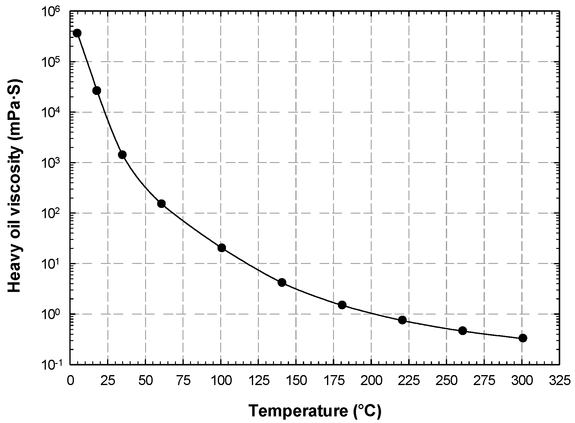
The oil properties in this area are listed in Table 2. The oil is live oil with an initial gas oil ratio (GOR) of 8.0 Sm3/m3 under the initial reservoir temperature of 18 °C and the average pressure of 3350 kPa. The salinity of the acquire is 44,000 PPM [11,12,14,31,32,33,34]. In addition, the viscosity of the oil is reduced remarkably with temperature increasing, which was simulated by using the CMG software [35], as shown in Figure 1.
3. Numerical Simulation Model
In this study, the commercial numerical simulator CMG STARS® (Computer Modelling Group Ltd., Calgary, AB, Canada) was employed to optimize the SAGD process in the reservoir with a bottom water zone. The basic numerical simulation model consisted of a 5-m active water zone directly below the oil zone, which is 20 m and covered by a 500-m overburden. A 3-D model was developed measuring 60 m in width with a grid size of 2 m (I direction), 25 m in height with a grid size of 1 m (including a 20 m oil pay zone and a 5 m bottom water zone; K direction), and 1000 m in length with a grid size of 20 m (J direction). In total, 37,500 grids were discretized. The 1000 meter-long horizontal SAGD well pair was drilled at the edge of the model along the J direction. For the base case, the thicknesses of the grid blocks were 1 m for both the oil pay zone and bottom water zone.
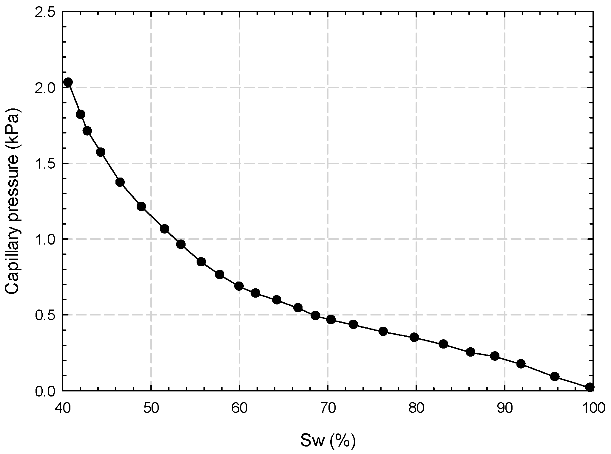
The SAGD well pair is a classic SAGD well pair, which indicates that the space between the two wells is 5 m, the producer is located 2.5 m above the bottom of the oil pay zone, and the well pair is drilled in a straight trajectory, the perforation of the wells are full perforated [35,39,40]. The reservoir is assumed to be homogeneous across both zones due to the main part of the reservoir being homogeneous [31].The relative permeability curves applied in the model are from a previous study on a heavy oil reservoir that is also operated by Husky Energy Ltd, Lloydminster, Canada, and is located very close to the Pikes Peak oil field in the Lloydminster region [41], as indicated in Table 3. The capillary pressure in the heavy oil reservoir is small, as shown in Figure 2 [42]. The start-ups of the SAGD processes are the same for all of the cases. First, (1) the duration of the preheating process lasts 75 days under 250 °C. Second, the steam trap control is 10 °C. Third, the temperature of the steam is 250 °C and the steam quality is 0.9 [43,44,45,46,47,48]. The maximum production rate is 550 m3/day, which is the capacity of the production pump used in this field. Also, the boundary condition of the numerical simulation model is a closed boundary.
4. Results and Discussion
4.1. Steam Injection Pressure Optimization
When the SAGD process is applied in a reservoir with a bottom water zone, the most serious issue is that the bottom water will invade the oil pay zone and be produced from the producer. Thus, the existence of a bottom water zone has a negative effect on heavy oil production performance [15,49,50].
In this study, in order to optimize the steam injection pressure, a new parameter () is defined as the ratio of the oil recovery factor () over the water production ratio of the bottom water zone (), as indicated in Equation (1). The parameter shows the heavy oil production performance in terms of both the positive aspect (oil recovery factor) and negative aspect (bottom water production) at a certain condition. The larger the parameter, the better the production performance obtained:
where is the defined parameter, dimensionless; is the oil recovery factor, %, equal to the cumulative oil production/the total original oil in place; and is the water production ratio from the bottom water zone, %, equal to the cumulative water production from the bottom water zone/initial water volume in the bottom water zone.
The values for each case can be calculated using Equation (2), which is derived from a previous study [51]. During the derivation process, one important assumption is considered: the chlorides concentration of the connect water remains constant, and it equals the initial chlorides concentration in the reservoir:
where is the water production ratio in the bottom water zone, %; is the water production volume from the bottom water zone, m3; is the total water volume in the bottom water zone, m3; is the water production volume from the entire reservoir, m3; is the water salinity in the produced water, ppm; is the initial water salinity in the bottom water zone, ppm; is the water cut, %; is the connate water saturation, %; and is the initial oil saturation, %.
In total, 14 cases are conducted in this section to optimize the steam injection pressure. The injection pressure ranges from 3350 kPa, which is the initial reservoir pressure, to 4000 kPa. The interval between the adjacent pressures is 50 kPa. Based on the calculated values, a correlation is developed. Equation (3) indicates the relationship between the steam injection pressure () and the defined factor (). The value (0.9804) shows a good correlation for the process, as shown in Figure 3.
Figure 3 indicates that a logarithm relation was obtained between the steam injection pressure and the value. The maximum of the value was achieved under the steam injection pressure at 3350 kPa, which is the initial reservoir pressure. The curve indicates that, with steam injection pressure increases, the oil production performance of the SAGD process applied in the heavy oil reservoir with a bottom water zone becomes worse due to the water coning effect growing stronger under a higher steam injection pressure [13]. Therefore, the well constraints for the base case can be indicated as: (1) the pressure constraint is 3350 kPa for the injector and (2) the fluid flow rate constraint is 550 m3/d for the producer and (3) the steam trap in the steam-trapping mode is 10 °C.
4.2. Effect of the Initial Gas Oil Ratio
The existence of the initial solution gas in the heavy oil has a significant impact on the oil production performance. Even the gas oil ratio is much smaller than that in the conventional oil reservoir [52]. In order to investigate the effects of the initial solution gas in the Pikes Peak reservoir, nine cases are developed, among which the initial GOR ranges from 0 to 8 Sm3/m3. The results of the simulation indicate that both positive and negative impacts of the initial solution gas appearing in the heavy oil reservoir are obtained in the SAGD process. The well constraints are the same as those in the base case.
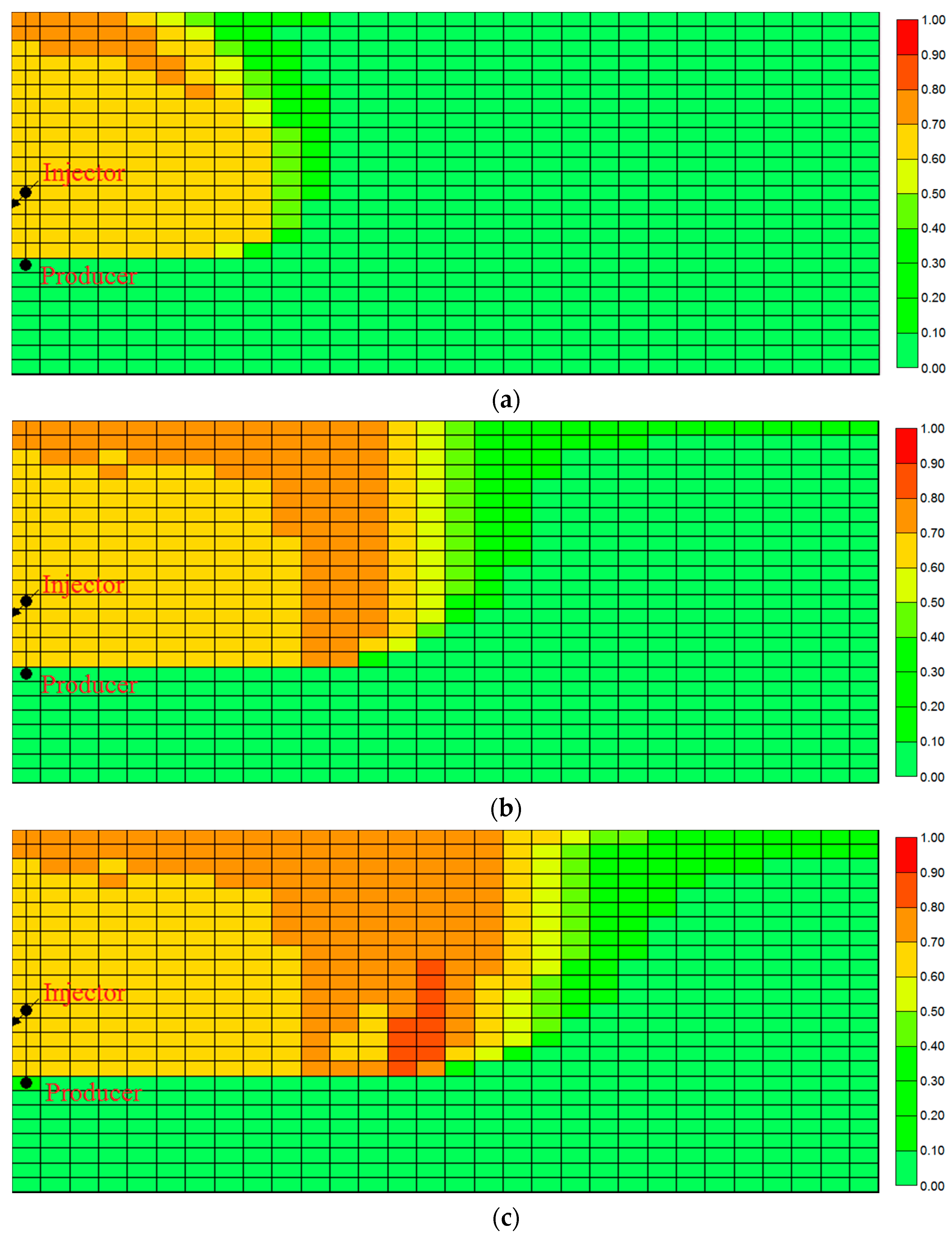
In the SAGD process, the temperature of heavy oil increases when high temperature steam is injected into the reservoir. The temperature increase leads to part of the solution gas being released from the heavy oil and rising to the top of the steam chamber (when the temperature is higher enough to make the heavy oil as saturated heavy oil), due to the gravity difference between the liquid phase and the gas phase. Thus, a gas bank is established at the top of the heated area, as shown in Figure 4. The size of the gas bank increases with injection time increases. Figure 4 manifests that the higher gas saturation always appears in front of the steam chamber due to the injected steam heating the inner part of the steam chamber, so that the temperature in the inner area of the steam chamber is much higher than that in other parts. Consequently, the gas oil ratio is lower in the inner area, and the injected steam pushes the exsoluted gas out of the inner area of the steam chamber. When the gas reaches the edge of the steam chamber, the mass transfer rate of the gas decreases dramatically because of the low temperature and the very high viscosity of the heavy oil. This decrease in mass transfer rate causes gas to accumulate in the front of the steam chamber.
Because the thermal conductivity of the gas phase is much lower than that of the liquid phase, the gas bank performs as an insulation layer to the overburden. Consequently, less heat loss occurs in the reservoir than it does in a reservoir without initial solution gas, as shown in Figure 5. This phenomenon was also observed in previous researches [53,54,55]. Figure 5 indicates that, the lower the initial GOR, the greater the heat loss to the overburden, which means that, with a lower initial GOR, the volume of the gas bank is smaller so that more heat can pass through the gas bank and be lost to the overburden. When the initial GOR reaches 5 Sm3/m3, the heat loss to the overburden does not increase significantly because the volume of the gas bank reaches a critical value under which the heat cannot be transferred efficiently. When the initial GOR is higher than 5 Sm3/m3, even the volume of the gas bank increases. The efficiency of the insulation cannot be improved too much, so the heat loss cannot be reduced significantly.
On the contrary, the gas bank not only reduces the heat loss to the overburden, but it also decreases the heat transfer ratio between the steam chamber and the oil reservoir. Consequently, a lower oil recovery factor is obtained when solution gas exists in the heavy oil, as shown in Figure 6. The negative effects of the existence of the initial solution gas were briefly reported in the previous literature [56,57,58,59,60,61,62,63,64,65,66,67,68,69]. In this study, more details are investigated.
Figure 6 manifests that, first, with initial GOR increases, the oil recovery factor decreases mainly because, the higher the initial GOR, the larger the volume of the gas bank that forms in front of the steam chamber. Thus, a smaller portion of the injected heat is transferred from the steam chamber to the oil reservoir.
Second, the oil recovery factor changes significantly in the initial GOR range of 2–5 Sm3/m3, but it does not change significantly under a low (0–2 Sm3/m3) and high (5–8 Sm3/m3) initial GOR. The reason for this is that, when the initial GOR is lower than 2 Sm3/m3, the volume of the gas bank is not large enough to establish an insulation layer to reduce the heat transfer efficiently. When the initial GOR is higher than 2 Sm3/m3, the volume of the gas bank increases with the initial GOR increases, and the efficiency of the insulation layer between the steam chamber and the overburden is improved, so that the heat loss to the overburden is reduced and more steam is applied to heat the cold heavy oil. Therefore, a higher oil recovery factor is obtained under the higher initial solution GOR. When the critical solution GOR is reached (5 Sm3/m3), the gas bank can reduce the heat transfer efficiently and the injected energy cannot be transferred into the further part of the reservoir. Consequently, the oil recovery factor does not increase significantly.
Third, the oil recovery factor with solution gas in the heavy oil is higher than that without solution gas in the early stage of the production process. This occurs because, at the early stage of the SAGD process, without initial GOR, the steam chamber increases vertically and cannot heat a large area of the heavy oil. When the solution gas appears in the oil reservoir, the gas saturation at the top of the steam chamber is higher than that in the other parts (as shown in Figure 4a), so that the heat transfer in the vertical direction is reduced and the steam chamber increases in both vertical and lateral directions. This leads to a larger area of the oil reservoir being heated. Consequently, the oil recovery factor is higher than that without initial solution gas.
4.3. Effect of Thickness of the Bottom Water Zone
In the Pikes Peak Waseca area, the thickness of the bottom water zone ranges from 0.3 m to 13.3 m, and the net pay of the oil zone reaches as high as 30 m. However, the lowest part of the oil pay zone is only 5 m [32]. Thus, the volume ratio of the bottom water zone to the oil pay zone (VRw/o) ranges from 0.01 to 2.66.
In order to study the effects of different sizes of the bottom water zone, various types of bottom water zones are created according to the VRw/o value. In this study, the thickness of the oil pay zone in the base case is 20 m. To meet the range of the VRw/o value, the thicknesses of the bottom water zone are developed from 0 m to 55 m. In total, 14 cases are developed to investigate the effect of the bottom water thickness. The interval is 5 m for the bottom water zone from 0 m to 55 m, and thicknesses of 1 m and 2.5 m are constructed to observe the effects of a very small bottom water zone. The well constraints in the section are the same as in the base case.
The relationships of the defined factor (Y), the bottom water production ratio (Rbw), and the volume of water produced from the bottom water zone (Qbw) under different thicknesses of the bottom water zone (hbw) are demonstrated in Figure 7. Through corrections, high corrections among Y, Rbw, Qbw, and hbw are obtained, as indicated in Equations (4)–(6). The corrections can be applied to analyze the effects of the properties of the bottom water zone:
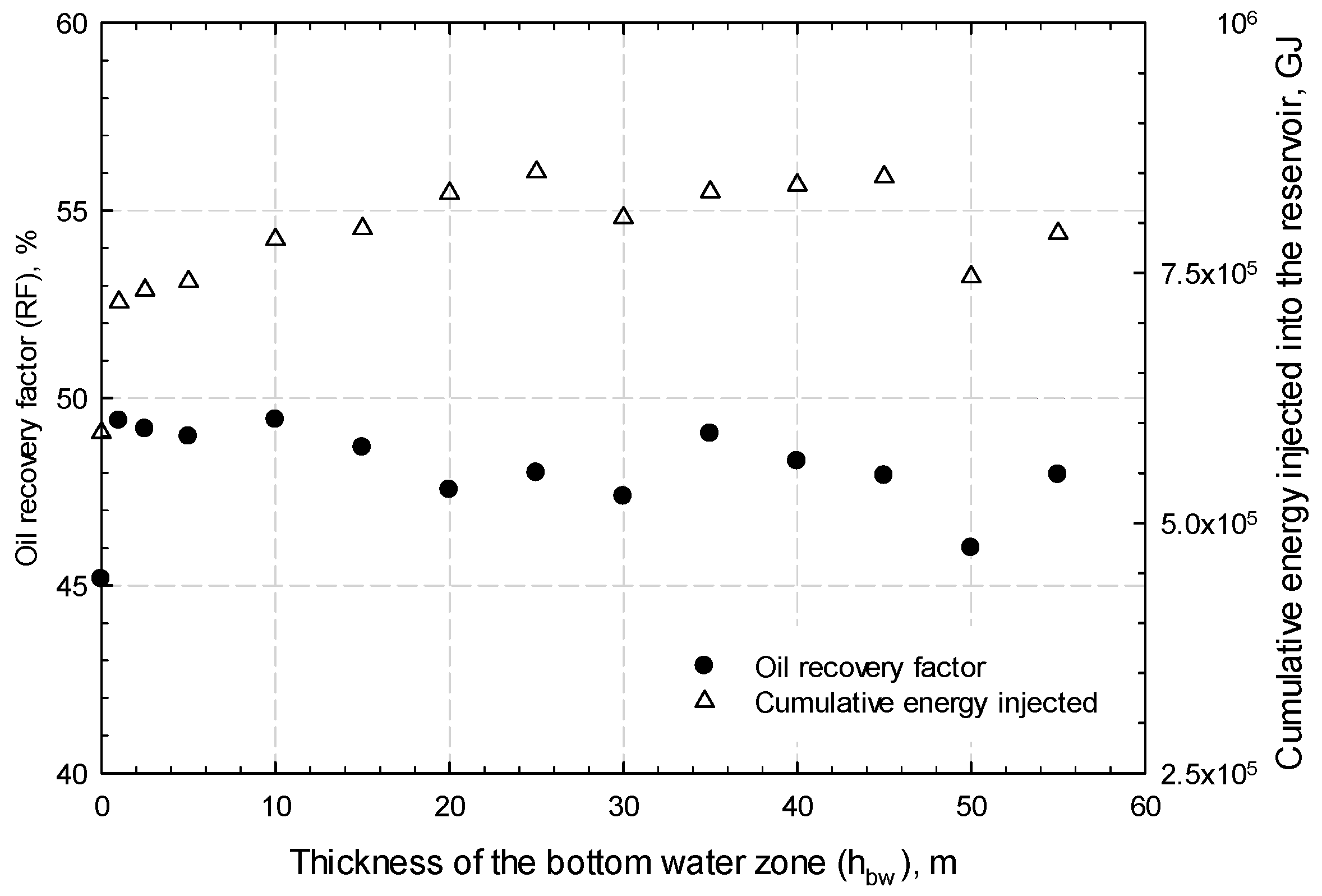
Figure 7 shows that the volume of water produced from the bottom water zone increases quickly with a lower thickness of the bottom water zone, but the incremental starts to decrease when the thickness increases to 20 m. That is mainly because: (1) the total volume of the bottom water zone increases proportional to the thickness and (2) the effect of the injection pressure (3350 kPa) to the thickness of the bottom water zone is around 20 m. When the thickness is higher than 20 m; the effect of the injection steam on the bottom water becomes weak. To be precise, the injected steam cannot push the water below 20 m in the bottom water zone. Consequently, the water production ratio in the bottom water zone (Rbw) decreases significantly before the hbw value is less than 20, but it decreases slowly when the thickness of the bottom water zone reaches 20 m. The Y value increases linearly with increases in the thickness of the bottom water zone due to: (1) the water production from the bottom water zone imminent a linear relation with the thickness of the bottom water zone when the thickness reaches 20 m; (2) the volume of the bottom water zone increases linearly, so that the Rbw value decreases smoothly; and (3) the oil recovery factor does not change too much when the bottom water zone appears, as shown in Figure 8.
Figure 8 reveals that the oil recovery factor and cumulative energy injected into the oil reservoir without a bottom water zone are lower than those occurring in reservoirs with a bottom water zone due to the bottom water augmenting the expansion process of the steam chamber in the oil pay zone, as indicated in Figure 9. This result is opposite to that of the previous study [26], which showed that the oil recovery factor is reduced by 10% with the bottom water zone. This difference occurs mainly because, in the previous study, no solution gas was considered in the heavy oil so that the heat transfer rate would not be reduced and the steam chamber could extend freely [26]. Therefore, the pressure in the steam chamber was not maintained, and the steam could be injected continuously. When the steam chamber reached the bottom water zone, heat loss occurred and negative effects occurred [26]. However, in this study, solution gas was considered in the heavy oil, and the gas bank reduced the heat transfer and kept the steam in the inner part of the steam chamber. Thus, less steam was injected into the reservoir, but the bottom water performed as a means to extend the steam chamber, as indicated in Figure 9.
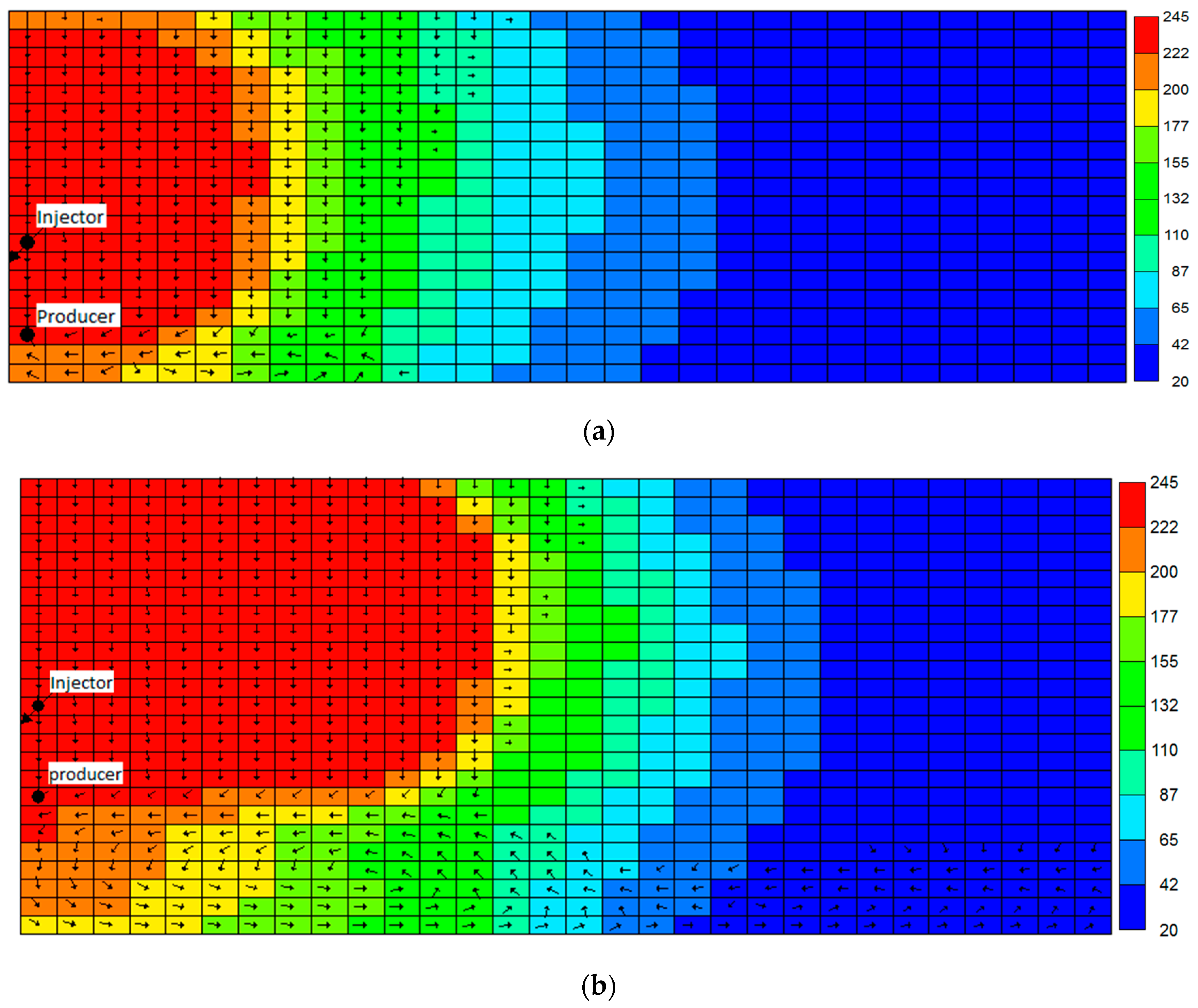
In Figure 9, the log value of water phase velocities in the reservoirs are highlighted to show the water phase flow direction in the reservoir. Without the bottom water zone (Figure 9a), the injected steam changes into the condensate water phase in the reservoir and flows towards the bottom of the reservoir. Then it is produced from the producer. Due to the negative effect of the gas bank, the heat transfer ratio of the steam chamber is lower, resulting in the lower volume of the steam chamber. Also, due to the well constraint (550 m3/day) of the producer, the condensate water phase cannot be produced immediately, which leads to the pressure in the steam chamber being maintained. Therefore, the volume of the steam (indicated by the injected energy) cannot be injected continuously. With the bottom water zone (Figure 9b), the condensate water phase would flow into the bottom water zone and circulate in it, carrying part of the energy with it. Also, the pressure in the steam chamber could be reduced and more steam could be injected into the reservoir to maintain the pressure. In addition, the energy that was taken by the water could be transferred to a further part of the bottom of the oil zone where it could help increase the temperature of the cold oil in front of the steam chamber. This temperature increase would increase the spread rate of the gas bank and result in a greater volume of the steam chamber.
4.4. Effect of Oil Saturation in the Bottom Water Zone
In the heavy oil reservoirs, lean zones (those located anywhere in a reservoir with low or no oil saturation zones) were found in Nexen’s Long Lake and Suncor’s Firebag SAGD projects. The effects of the existence of lean zones are remarkable in the SAGD process [50,70,71]. In this study, the bottom water zone is a typical lean zone in the heavy oil reservoir. In order to study the effects of the different oil saturations in the lean zone, six cases were developed. The range of the oil saturations in the lean zone changed from 0 to 0.5, and the thickness of the bottom water zone was the same as that of the base case, which is 5 m. The well constraints for the cases are same as the base case.
The incremental ratio of the parameters can be represented as follows:
where represents the Original Oil in Place (OOIP), Rbw, RF, and cEOR; is the incremental ratio of parameter ; and is the oil saturation in the bottom water zone.
With oil saturation increases in the bottom water zone, three phenomena are investigated. First, the Rbw increases over 10% (Rinc,Rbw = 10.748%) when oil (with a 10% oil saturation) appears in the bottom water zone. Then the ratio decreases when the oil saturation in the bottom water zone increases. Second, the RF increases a little bit before the oil saturation reaches 30%. Then it decreases with the oil saturation in the bottom water zone increases. Third, the cEOR decreases with increases in oil saturation in the bottom water zone. The major reason for this is that, with a small amount of oil in the bottom water zone, when the reservoir is heated by injected steam, the solution gas evolves from the oil. The evolved gas disperses in the heavy oil for a certain amount of time, and it partly decreases the viscosity and density of the fluids in the bottom water zone [8]. This decrease in viscosity and density leads to a relative higher mobility of the fluids (both water and oil) in the bottom water zone. Thus, the Rbw and the RF increase. As shown in Table 4.
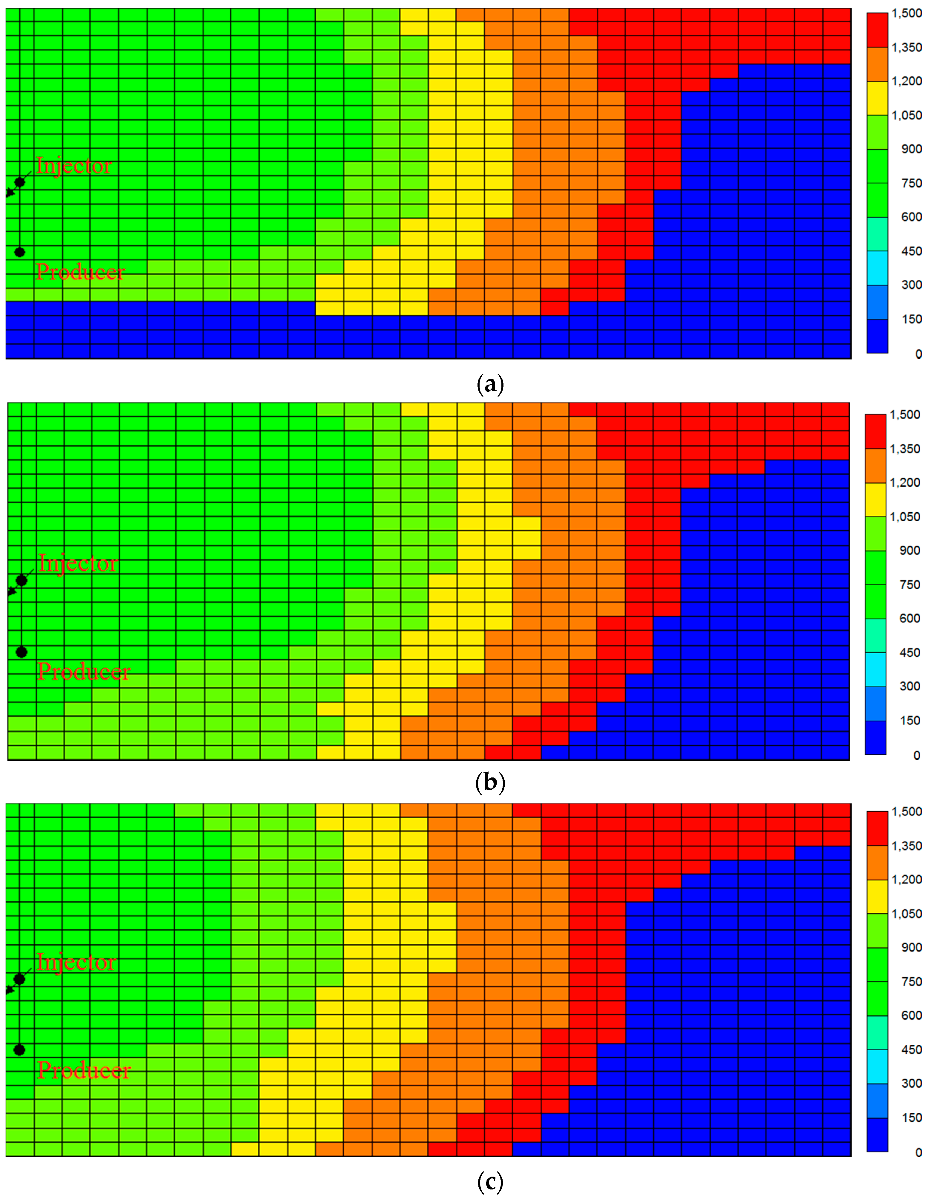
The mole density of the gas phase indicates gas phase distribution in the reservoir, as shown in Figure 10a,b. However, with the continual increase of oil saturation in the bottom water zone, the amount of free gas increases during the heating process (as indicated in Figure 10c). This results in the negative effect of the solution gas (the heat transfer rate is reduced by the gas bank) becoming increasingly more significant. Therefore, the Rbw and RF will decrease. For the cEOR, before the oil saturation reaches 30%, the oil recovery factors are higher than the case without oil in the bottom water zone, so the cEOR decreases. When the oil saturation in the bottom water zone is higher than 30%, the energy injected into the reservoir decreases due to the obstacle of the gas bank in the reservoir. This energy decrease causes the cEOR to decrease.
4.5. Effect of the Well Pair Location
To study the effect of the well pair location in the SAGD process, 13 cases are developed. Among these, the distance between the injector and producer in the horizontal well pair is kept constant (5 m). The location of the producer changes from the oil pay zone to the bottom water zone, and the distance between the producer and the original oil-water contactor is changed from 4.5 m (i.e., the producer is located 4.5 m above the original oil-water contact) to −4.5 m (i.e., the producer is located 4.5 m below the original oil-water contact).
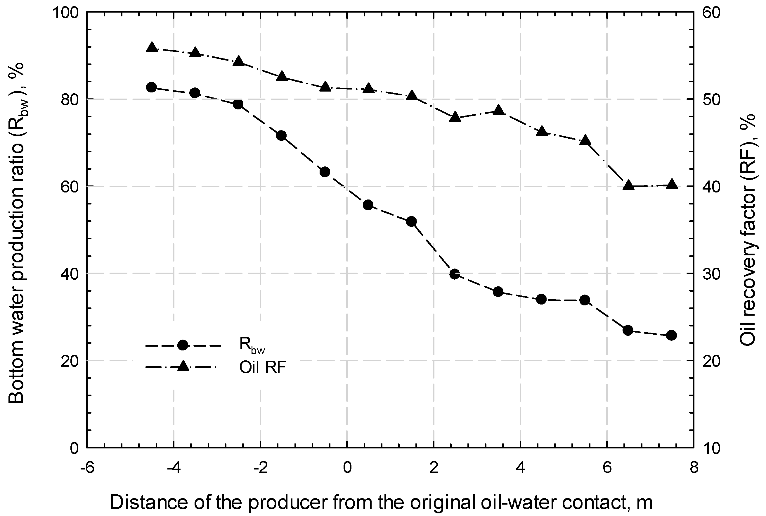
The results of parameters Rbw and RF are shown in Figure 11. The negative distance indicates that the producer is located below the original oil-water contact, and the positive distance shows that the producer is drilled above the original oil-water contact. Both Rbw and RF decrease when the producer location changes from the bottom of the reservoir upwards (i.e., when the producer location is −4.5 m). This decrease occurs because, the lower the well pair, the larger the area of the bottom water zone occupied by the steam chamber and the more water produced from the bottom water zone. Also, the area of the steam chamber in the oil pay zone is larger due to the shape of the steam chamber moving downwards and the wider part occupies the oil pay zone. Therefore, more oil will be heated and produced, which results in a higher RF.
If the well pair is moved upwards, the steam chamber moves towards the top of the reservoir. Therefore, less water in the bottom water zone can be produced, and the Rbw decreases quickly with the upward movement of the well pair. Also, the lower part of the steam chamber is moved to the oil pay zone, resulting in less area of the oil pay zone being heated. Therefore, the RF decreases.
4.6. Effect of Different Well Patterns
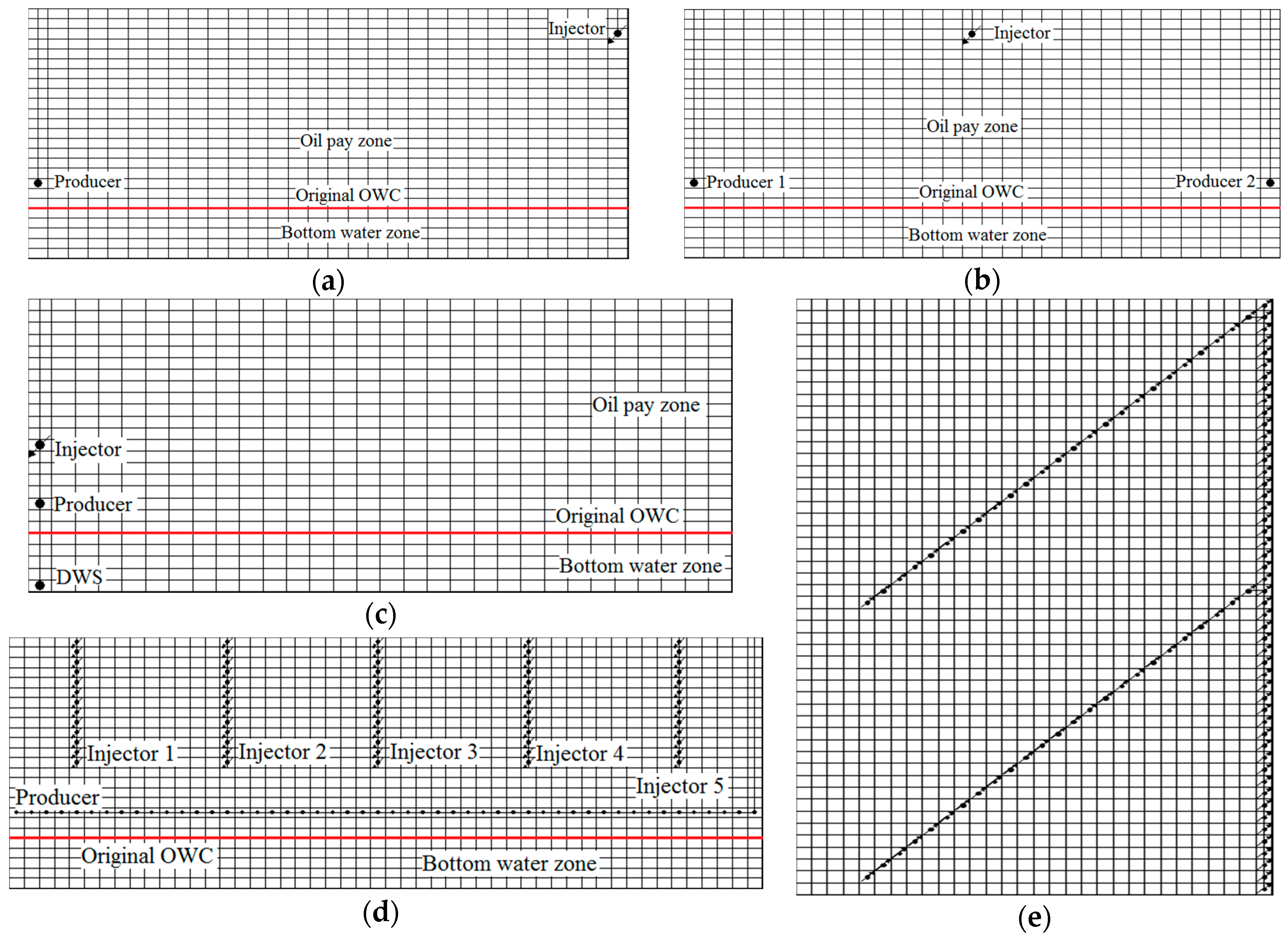
In order to study the effect of different well patterns in the production process in a heavy oil reservoir with a bottom water zone, five well patterns (two corner wells, triple wells, downhole water sink well (DWS), vertical injectors with a horizontal producer (VInj-HPro), and fishbone well) are conducted in the same reservoir with the same operation parameters. The well patterns are shown in Figure 12. Figure 12a,c show the I-K direction cross-section of the reservoir. Figure 12d indicates the J-K direction cross-section of the reservoir, while Figure 12e demonstrates the I-J direction cross-section of the reservoir. In order to gain a better view, the display length ratio for Figure 12e in the J direction to the I direction is revised to Y/X = 0.1 × J direction length: 1 × I direction length. For the two corner wells, as shown in Figure 12a, the producer is located in the boundary of the reservoir, which is the same place as the conventional SAGD process. The injector is drilled 2.5 m under the top boundary of the other boundary. For the triple wells, as shown in Figure 12b, the injector is located 2.5 m under the top boundary in the middle of the reservoir. One producer is drilled 2.5 m above the original oil-water contact on each boundary. For the DWS, as shown in Figure 12c, another producer is placed at the bottom of the reservoir under the conversational SAGD well pair. For the VInj-HPro, as shown in Figure 12d, five vertical injectors are drilled 5 m above the horizontal producer. For the fishbone well, as shown in Figure 12e, the locations of the main wells are the same as the location of the conventional SAGD well pair, and the well brunches are in the same layer as the main wells.
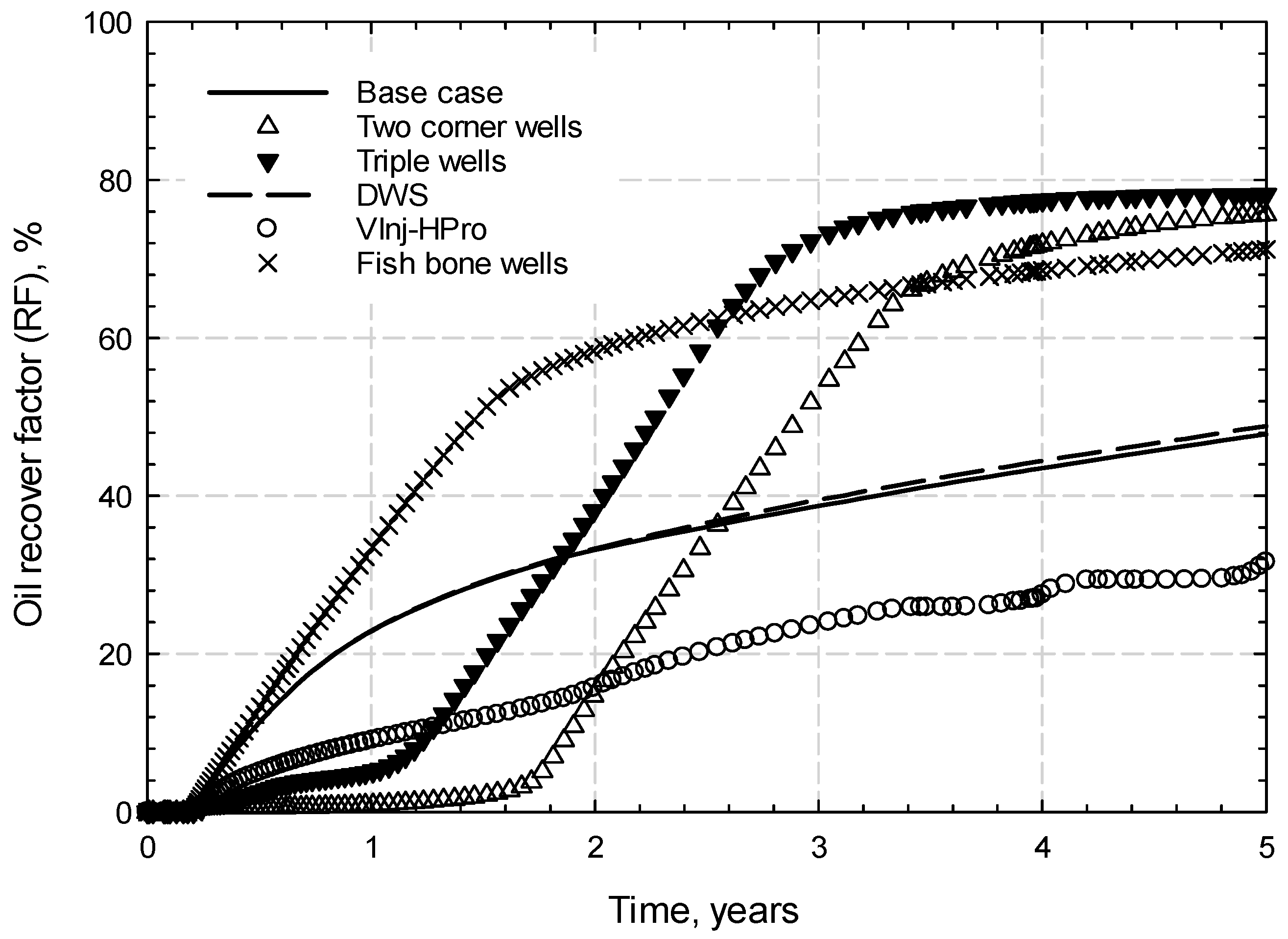
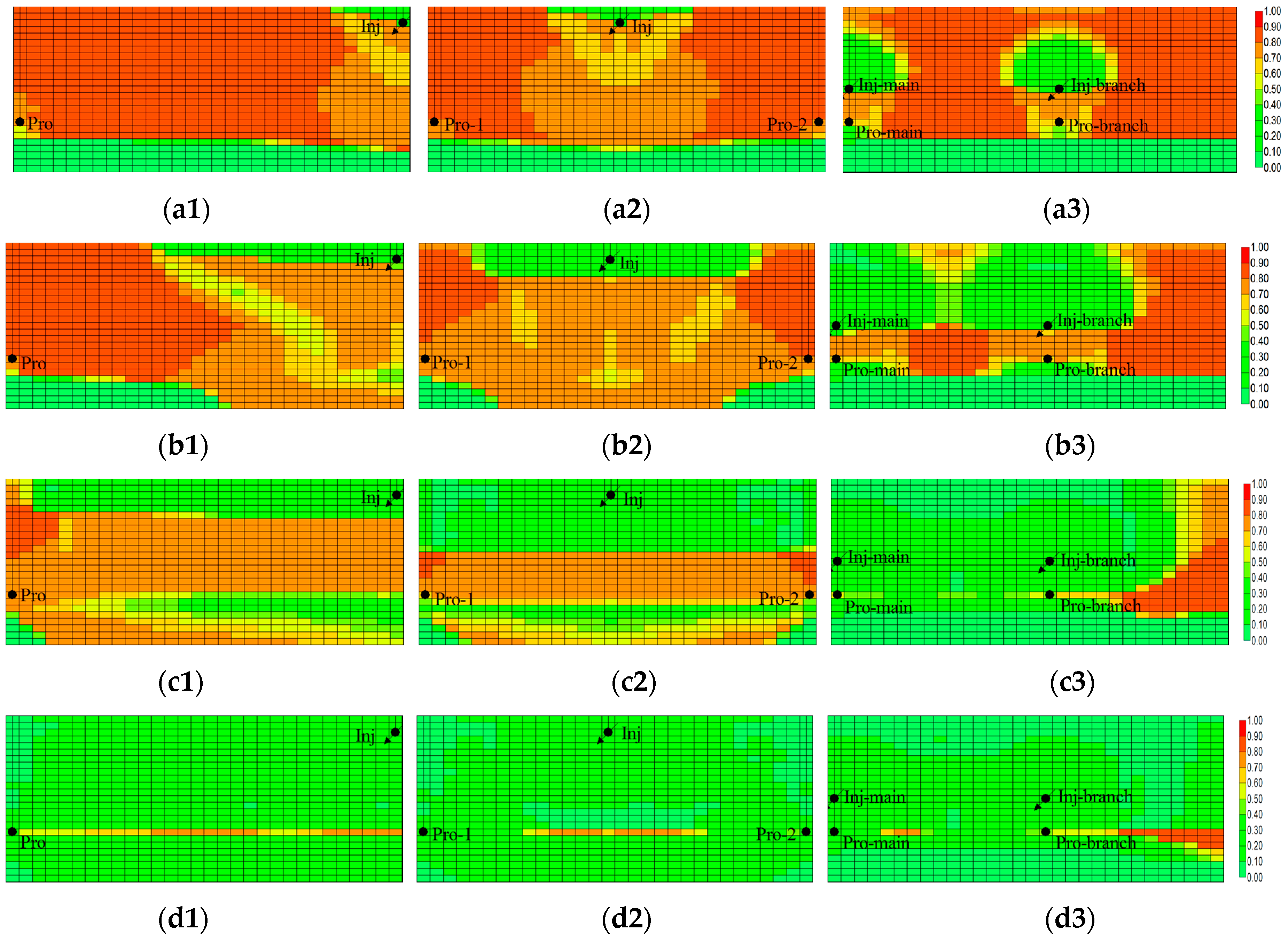
The oil recovery factors for different well patterns are shown in Figure 13. For the base case, the oil recovery factor is 47.84%, which is not high enough for a SAGD process [35]. When the two corner wells, triple wells, and fish bone well patterns were conducted, the oil production was enhanced significantly (as indicated in Figure 14d) to as high as 77.19%, which is 10% higher than the previous experimental study [18] when the triple wells pattern was applied. However, the start time of the oil production was delayed for the well patterns of two corner wells and triple wells. For the base case (the traditional SAGD well pattern), the oil production occurred at the time (75 days) when the preheating process ends. For the two corner wells pattern, the oil production time was delayed to 1.8 years. For the triple wells pattern, it was delayed to 1.2 years due to the long distance between the injector and the producer. Thus, the duration of the connection establishment process between the injector and the producer is longer than that in the conventional SAGD process, as shown in Figure 14(a1,a2).
Once the connection between the injector and the producer was established, the oil production rate (indicated by the slope of the oil recovery factor curve) increased significantly. Because of the viscosity difference between the heavy oil and the bottom water, part of the heavy oil in the oil pay zone was pushed into the bottom water zone before the connection process was achieved, as indicated in Figure 14(b1,b2). When the heat conduction process transferred the injected heat from the injector to the producer, a large amount of heated heavy oil was displaced to the producer due to the pressure difference between the injector and the producer together with the gravity effects. The condensate water flushed to the bottom water zone due to the density difference between the heavy oil and the condensate water. The amount of the invaded heavy oil in the bottom water zone did not increase when the injector and the producer connected to each other with the heated heavy oil, and the invaded higher temperature heavy oil was pushed to the producer by the condensate water in the bottom water zone. Therefore, an increase in the water phase was observed in the area between the oil pay zone and the invaded heavy oil, as shown in Figure 14(c1,c2).
For the fishbone well pattern, the main reason for the higher oil recovery rate is that the fishbone wells, including the main wells and the branches, extend the heating area in the reservoir, as shown in Figure 12e. The branches of the fishbone wells reach the further part of the reservoir and distribute the steam in that region, so that the temperature of the heavy oil in that area can be improved and the viscosity will be decreased significantly. This leads to the heavy oil production process occurring in the branches, as shown in Figure 14(a3), so that the heavy oil around the main wells and the branches are heated and produced. When the oil recovery factor reaches 60%, the heavy oil production rate decreases quickly, and the heavy oil recovery factor curve tends towards flat due to the heavy oil around the fishbone wells being produced. It is hard for the injected steam to heat the heavy oil in the further part of the reservoir. Therefore, the production process can be stopped at the second year. For the same reason, if the two corner wells and triple wells patterns are conducted, the production process can be ended at 3 years and 3.5 years, respectively, rather than 5 years.
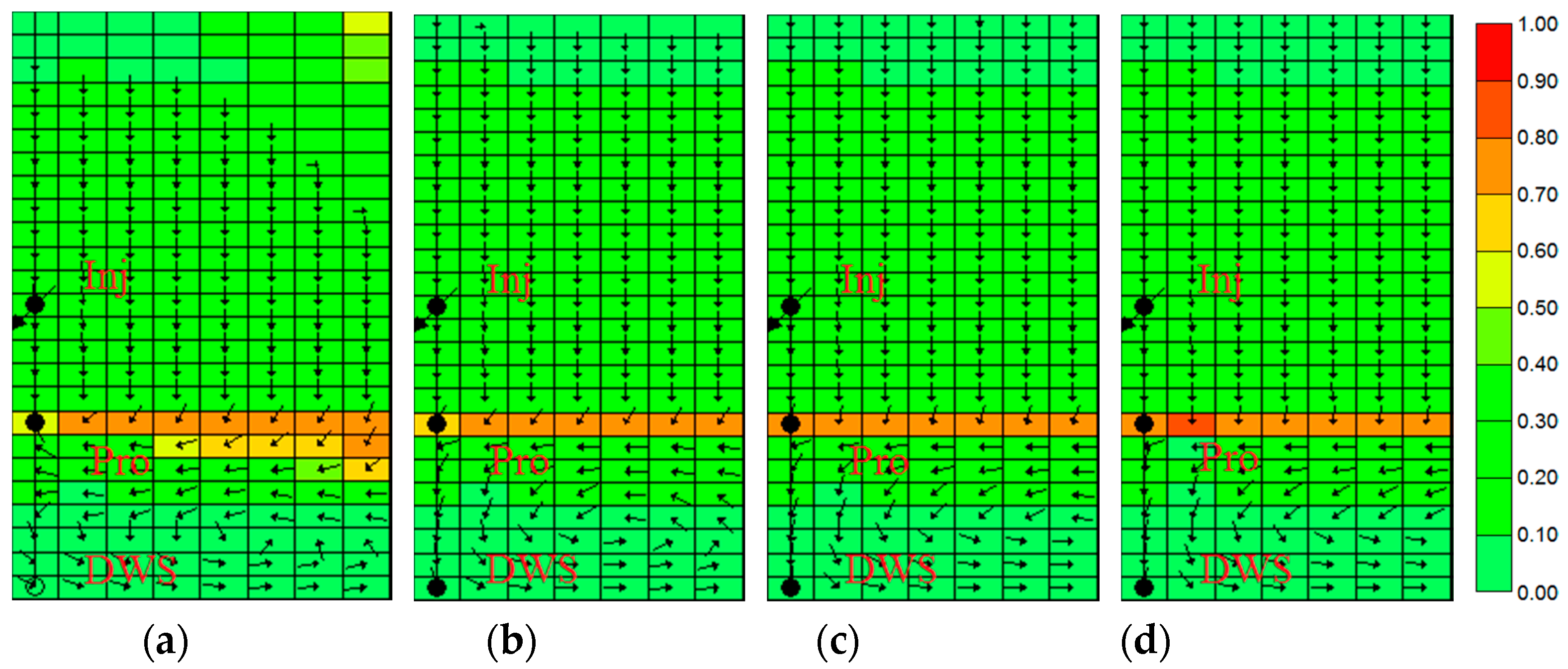
For the DWS well pattern, the pressure constraint of the DWS is 3428 kPa. Compared with the conventional SAGD process, the oil recovery factor of the DWS well pattern is slightly higher than that of the base case, which is the conventional SAGD process, as shown in Figure 13. However, the water cut reduced sharply to around 2% when the DWS started to produce water from the bottom water zone, as indicated in Figure 15. This reduction in water cut occurred due to the pressure of the bottom water zone decreasing to 3428 kPa, which is the maximum pressure in the DWS well constraint. Also, the pressure constraint in the DWS is very sensitive to the water production start time of the DWS, as an increment of as much as 1 kPa occurred. The start time was delayed for about half a year for the pressure under 3426 kPa to 3428 kPa, but an almost 1.5 year delay occurred when the pressure increased from 3428 kPa to 3429 kPa. The key reason for this is that, in the SAGD process, the injected steam maintains the pressure in the oil pay zone. With the effect of gravity, the pressure at the bottom of the reservoir, where the DWS located, is thus higher than that in the oil zone, and it increases with the amount of steam injected. When the pressure is higher than the pressure constraints in the DWS, the bottom water is produced from the DWS and the pressure in the bottom water zone remains the same as the pressure constraints of the DWS. Due to the pressure decreases in the bottom water zone, the pressure difference between the bottom water zone and the producer is reduced and it cannot support the energy for the water flux to the producer. Therefore, the water cut decreases extremely. This is the key benefit of the DWS well pattern: even the oil recovery factor does not increase too much.
As shown in Figure 16, before the DWS well pattern started to produce bottom water, it was under an inactive status. Thus, the bottom water flowed to the producer because higher pressure in the bottom water zone was obtained with the effect of the gravity of the condensate water, and the water flowed in a circular flow. When the pressure in the bottom water zone increased to the well constraint pressure, the bottom water started to flow towards the DWS rather than toward the producer, as indicated in Figure 16b. As time went by, the condensate water flow direction changed vertically to the bottom water zone in the bottom of the oil pay zone and fluxed towards the DWS. Therefore, less water flowed to the producer and a lower water cut was obtained.
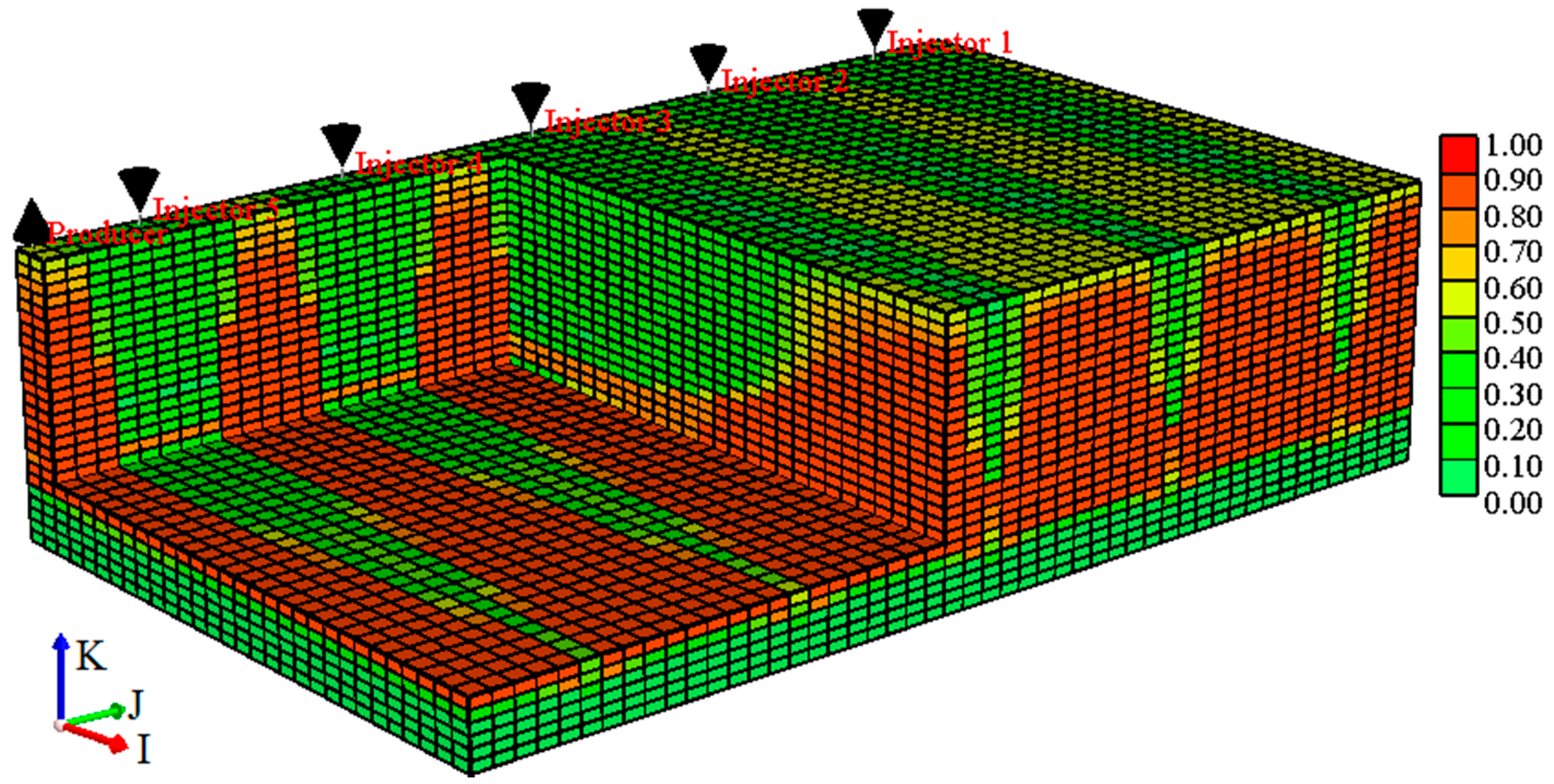
For the VInj-HPro well pattern, the lowest oil recovery factor (31.18%) was gained among the five well patterns, as shown in Figure 13. The reason for the lower oil recovery factor even through five vertical injectors were conducted in the reservoir is that the heat conduction process occurs around the injectors and the size of the steam chamber grows smaller with the depth increases. Due to the effect of the steam gravity overriding, the results in the residual oil saturation in the top part of the reservoir are much lower than that in the bottom part of the oil pay zone. The established free gas bank in front of the steam chamber weakens the heat conduction process, which means the heat transfer rate is decreased. Thus, the steam chamber cannot cover the space among the injectors. As shown in Figure 17, a large amount of oil remained in the area between the adjacent injectors. Therefore, the oil recovery rate is lower than that in other well patterns. To obtain a better view of the oil distribution in the oil reservoir, the display length ratio in the J direction to the I direction was modified to Y/X = 0.1 × J direction length: 1 × I direction length.
5. Conclusions
Six conclusions can be drawn from this study. First, for the heavy oil reservoir with a bottom water zone, the steam injection pressure affects the water production ratio from the bottom water zone dramatically. An optimized injection pressure can increase the defined value to a maximum value, which indicates a better production performance than in other cases.
Second, both positive and negative effects are observed in the reservoir with solution gas. The positive effect reduces the heat loss to the overburden because of the gas layer on the top of the oil pay zone. But the free gas bank in front of the steam chamber, like an insulation layer, reduces the heat transfer rate in the reservoir, which leads to the reduction of the injected heat utilization.
Third, with the thickness of the bottom water zone increasing, the oil recovery factor decreases a little bit, and logarithmical relationships are investigated between the volumes of the bottom water production, bottom water production ratio, and the thickness of the bottom water zone.
Fourth, as a lean zone, the oil saturation in the bottom water zone can increase the oil recovery rate when the oil saturation is not very high. Then it decreases after the oil saturation reaches 30% and the cumulative energy oil ratio decreases when the oil saturation in the bottom water zone increases.
Fifth, a higher oil recovery factor can be obtained when a lower well location is applied in the reservoir. When the producer is drilled in the bottom water zone, the oil recovery factor is higher than that when the producer is drilled in the oil pay zone. Nevertheless, the water production ratio from the bottom water zone increases significantly when the producer is located in the bottom water zone.
Sixth, compared to five different well patterns, the two corner wells and triple wells patterns can gain the highest oil recovery factors (74.71% and 77.19%, respectively), which are almost twice that achieved in the conventional SAGD process (47.84%), and the main production duration is shortened.
Author Contributions
Xiang Zhou established the numerical model and designed the research; Jun Ni run the simulation cases and studied the applicability of simulation method in heavy oil reservoir with bottom water zone; Qingwang Yuan and Xinqian Lu conceived the integrated simulation approach described in Section 4.1, Section 4.2, Section 4.3; Fanhua Zeng and Keliu Wu performed the research in Section 4.6 and analyzed simulation results; Xiang Zhou and Jun Ni wrote this paper.
Conflicts of Interest
The authors declare no conflict of interest.
References
- Gates, I.D.; Larter, S.R. Energy efficiency and emissions intensity of SAGD. Fuel 2014, 115, 706–713. [Google Scholar] [CrossRef]
- Hsu, C.; Robinson, P. Practical Advances in Petroleum Processing; Springer: New York, NY, USA, 2006. [Google Scholar]
- Selby, R.; Alikhan, A.A.; Ali, S.M.F. Potential of non-thermal methods for heavy oil recovery. J. Can. Pet. Technol. 1989, 28, 45–59. [Google Scholar] [CrossRef]
- Wang, L.; Liu, H.; Pang, Z.; Lv, X. Overall heat transfer coefficient with considering thermal contact resistance in thermal recovery wells. Int. J. Heat Mass Transf. 2016, 103, 486–500. [Google Scholar] [CrossRef]
- Zhao, W.D.; Wang, J.; Gates, I.D. Thermal recovery strategies for thin heavy oil reservoirs. Fuel 2014, 117, 431–441. [Google Scholar] [CrossRef]
- Zhu, Z.; Zeng, F.; Zhao, G.; Laforge, P. Evaluation of the hybrid process of electrical resistive heating and solvent injection through numerical simulations. Fuel 2013, 105, 119–127. [Google Scholar] [CrossRef]
- Zhou, X.; Zeng, F. Feasibility study of using polymer to improve SAGD performance in oil sands with top water. In Proceedings of the SPE Heavy Oil Conference, Calgary, AB, Canada, 10–12 June 2014. [Google Scholar] [CrossRef]
- Zhou, X.; Zeng, F.; Zhang, L.; Wang, H. Foamy oil flow in heavy oil—Solvent systems tested by pressure depletion in a sandpack. Fuel 2016, 171, 210–223. [Google Scholar] [CrossRef]
- Boyle, T.B.; Gittins, S.D.; Chakrabarty, C. The evolution of SAGD technology at East Senlac. J. Can. Pet. Technol. 2003, 42, 58–61. [Google Scholar] [CrossRef]
- Butler, R.M. Some recent development in SAGD. J. Can. Pet. Technol. 2001, 40, 18–22. [Google Scholar] [CrossRef]
- Miller, K.A. Interim progress report on Husky’s Pikes Peak steam pilot. J. Can. Pet. Technol. 1986, 25, 42–46. [Google Scholar] [CrossRef]
- Miller, K.A.; Steiger, R. Pikes peak project: Successful without horizontal wells. J. Can. Pet. Technol. 1999, 38, 21–26. [Google Scholar] [CrossRef]
- Sugianto, S.; Butler, R.M. The production of conventional heavy oil reservoirs with bottom water using steam-assisted gravity drainage. J. Can. Pet. Technol. 1990, 29, 78–86. [Google Scholar] [CrossRef]
- Watson, I.A.; Brittle, K.F.; Lines, L.R. Heavy-oil reservoir characterization using elastic wave properties. Lead. Edge 2001, 13, 777–784. [Google Scholar] [CrossRef]
- Jiang, Q.; Butler, R.M. Experimental and numerical modelling of bottom water coning to a horizontal well. J. Can. Pet. Technol. 1998, 37, 82–91. [Google Scholar] [CrossRef]
- Falk, K.; Nzekwu, B.; Karpuk, B.; Pelensky, P. A review of insulated concentric coiled tubing installations for single well, steam assisted gravity drainage. In Proceedings of the SPE Gulf Coast Section/ICoTA North American Coiled Tubing Roundtable, Conroe, TX, USA, 26–28 February 1996. [Google Scholar] [CrossRef]
- Doan, L.T.; Baird, H.; Doan, Q.T.; Ali, S.M.F. An investigation of the steam-assisted gravity-drainage process in the presence of a water leg. In Proceedings of the SPE Annual Technical Conference and Exhibition, Houston, TX, USA, 3–6 October 1999. [Google Scholar] [CrossRef]
- Huygen, H.H.A.; Lowry, W.E. Steamflooding Wabasca tar sand through the bottomwater zone—Scaled mModel tests. Soc. Pet. Eng. J. 1983, 23, 92–98. [Google Scholar] [CrossRef]
- Proctor, M.L.; George, A.E.; Ali, S.M.F. Steam injection strategies for thin, bottom water reservoirs. In Proceedings of the SPE California Regional Meeting, Ventura, CA, USA, 8–10 April 1987. [Google Scholar] [CrossRef]
- Swisher, M.D.; Wojtanowicz, A.K. New dual completion method eliminates bottom water coning. In Proceedings of the SPE Annual Technical Conference and Exhibition, Dallas, TX, USA, 22–25 October 1995. [Google Scholar] [CrossRef]
- Jespersen, P.J.; Fontaine, T.J.C. The tangleflags North pilot: A horizontal well steamflood. J. Can. Pet. Technol. 1993, 32, 52–57. [Google Scholar] [CrossRef]
- Miller, K.A.; Xiao, Y. Lloydminster, Saskatchewan vertical well SAGD field test results. J. Can. Pet. Technol. 2010, 49, 22–29. [Google Scholar] [CrossRef]
- Hocking, G.; Cavender, T.W.; Person, J.; Hunter, T. Single-well SAGD field installation and functionality trials. In Proceedings of the SPE Heavy Oil Conference, Calgary, AB, Canada, 12–14 June 2012. [Google Scholar] [CrossRef]
- Shirman, E.I.; Wojtanowicz, A.K. More oil using downhole water-sink technology: A feasibility study. SPE Prod. Facil. 2000, 15, 234–240. [Google Scholar] [CrossRef]
- Masih, S.; Ma, K.; Sanchez, J.; Patino, F.; Boida, L. The effect of bottom water coning and its monitoring for optimization in SAGD. In Proceedings of the SPE Heavy Oil Conference, Calgary, AB, Canada, 12–14 June 2012. [Google Scholar] [CrossRef]
- Dong, X.; Liu, H.; Zhang, Z.; Lu, C.; Fang, X.; Zhang, G. Feasibility of the steam-assisted-gravity-drainage process in offshore heavy oil reservoirs with bottom water. In Proceedings of the Offshore Technology Conference, Houston, TX, USA, 5–8 May 2014. [Google Scholar]
- Doan, L.T.; Baird, H.; Doan, Q.T.; Ali, S.M.F. Performance of the SAGD process in the presence of a water sand—A preliminary investigation. J. Can. Pet. Technol. 2003, 42, 25–31. [Google Scholar] [CrossRef]
- Qin, W.; Wojtanowicz, A.K.; Li, H. Improved thermal heavy oil recovery from strong bottom-water-drive reservoir by combining SAGD with downhole water sink. In Proceedings of the SPE International Heavy Oil Conference and Exhibition, Mangaf, Kuwait, 8–10 December 2014. [Google Scholar] [CrossRef]
- Munoz, R. Simulation sensitivity study and design parameters optimization of SAGD process. In Proceedings of the SPE Heavy Oil Conference, Calgary, AB, Canada, 11–13 June 2013. [Google Scholar] [CrossRef]
- Peterson, J.; Riva, D.T.; Connelly, M.E.; Solanki, S.C.; Edmunds, N.R. Conducting SAGD in shoreface oil sands with associated basal water. J. Can. Pet. Technol. 2010, 49, 74–79. [Google Scholar] [CrossRef]
- Miller, K.A.; Given, R. Evaluation and application of Pikes Peak cyclic steam injection pressure data. J. Can. Pet. Technol. 1989, 28, 26–32. [Google Scholar] [CrossRef]
- Wong, F.Y.F.; Anderson, D.B.; O’Rourke, J.C.; Rea, H.Q.; Scheidt, K.A. Meeting the challenge to extend success at the Pikes Peak steam project to areas with bottom water. SPE Reserv. Eval. Eng. 2003, 6, 157–167. [Google Scholar] [CrossRef]
- Miller, K.A.; Xiao, Y. Improving the performance of classic SAGD with offsetting vertical producers. J. Can. Pet. Technol. 2008, 47, 22–27. [Google Scholar] [CrossRef]
- Zhou, X.; Zeng, F.; Zhang, L. Improving steam-assisted gravity drainage performance in oil sands with a top water zone using polymer injection and the fishbone well pattern. Fuel 2016, 184, 449–465. [Google Scholar] [CrossRef]
- Computer Modelling Group Ltd. Computer Modelling Group STARTS User Manual; Computer Modelling Group Ltd.: Calgary, AB, Canada, 2016. [Google Scholar]
- Dusseault, M.B. Comparing Venezuelan and Canadian heavy oil and tar sands. In Proceedings of the Canadian International Petroleum Conference, Calgary, AB, Canada, 12–14 June 2001. [Google Scholar] [CrossRef]
- Butler, R.M. Thermal recovery of oil and bitumen. In Englewood Cliffs; Prentice-Hall: Upper Saddle River, NJ, USA, 1991. [Google Scholar]
- Akbarzadeh, K.; Dhillon, A.; Svrcek, W.Y.; Yarranton, H.W. Methodology for the characterization and modeling of Asphaltene precipitation from heavy oils diluted with n-Alkanes. Energy Fuels 2004, 18, 1434–1441. [Google Scholar] [CrossRef]
- Tamer, M.; Gates, I.D. Impact of different SAGD well configurations (Dover SAGD phase B case study). J. Can. Pet. Technol. 2012, 1, 32–45. [Google Scholar] [CrossRef]
- Su, Y.; Wang, J.Y.; Gates, I.D. SAGD well orientation in point bar oil sand deposit affects performance. Eng. Geol. 2013, 157, 79–92. [Google Scholar] [CrossRef]
- Karajgikar, A. Thermal Recovery of Heavy Oil Using Pressure Pulses of Injected Syngas. Ph.D. Thesis, University of Calgary, Calgary, AB, Canada, 2015. [Google Scholar]
- Qin, W. Analytical Design Method for Cold Production of Heavy Oil with Bottom Water Using Bilateral Sink Wells. Ph.D. Thesis, Louisiana State University, Baton Rouge, LA, USA, 2011. [Google Scholar]
- Edmunds, N. Investigation of SAGD steam trap control in two and three dimensions. J. Can. Pet. Technol. 2000, 39, 30–40. [Google Scholar] [CrossRef]
- Shin, H.; Polikar, M. Review of reservoir parameters to optimize SAGD and fast-SAGD operating conditions. J. Can. Pet. Technol. 2007, 46, 30–40. [Google Scholar] [CrossRef]
- Ivory, J.J.; Zheng, R.; Nasr, T.N.; Deng, X.; Beaulieu, G.; Heck, G. Investigation of low pressure ES-SAGD. In Proceedings of the International Thermal Operations and Heavy Oil Symposium, Calgary, AB, Canada, 20–23 October 2008. [Google Scholar] [CrossRef]
- Dickson, J.L.; Clingman, S.; Dittaro, L.M.; Jaafar, A.E.; Yerian, J.A.; Perlau, D. Design approach and early field performance for a solvent-assisted SAGD pilot at Cold Lake, Canada. In Proceedings of the SPE Heavy Oil Conference and Exhibition, Kuwait City, Kuwait, 12–14 December 2011. [Google Scholar] [CrossRef]
- Gotawala, D.R.; Gates, I.D. A basis for automated control of steam trap subcool in SAGD. SPE J. 2012, 17, 680–686. [Google Scholar] [CrossRef]
- Miller, K.A.; Xiao, Y. Field results for recovering oil from a steam-project pressure-insulation wall. J. Can. Pet. Technol. 2013, 52, 368–375. [Google Scholar] [CrossRef]
- Ju, B.; Qiu, X.; Dai, S.; Fan, T.; Wu, H.; Wang, X. A study to prevent bottom water from coning in heavy-oil reservoirs: Design and simulation approaches. J. Energy Resour. Technol. 2008, 130, 033102. [Google Scholar] [CrossRef]
- Wang, C.; Leung, J.Y. Characterizing the effects of lean zones and shale distribution in steam-assisted-gravity-drainage recovery performance. SPE Reserv. Eval. Eng. 2015, 18, 329–345. [Google Scholar] [CrossRef]
- Masih, S.; Bennett, B.; Savage, M. The measurement of connate water chlorides concentration and its effect on bottom water coning analysis in SAGD for optimization. In Proceedings of the SPE Heavy Oil Conference, Calgary, AB, Canada, 10–12 June 2014. [Google Scholar] [CrossRef]
- Ardali, M.; Barrufet, M.; Mamora, D.D. Effect on non-condensable gas on solvent-aided SAGD processes. In Proceedings of the SPE Heavy Oil Conference, Calgary, AB, Canada, 12–14 June 2012. [Google Scholar] [CrossRef]
- Butler, R. The steam and gas push (SAGP). J. Can. Pet. Technol. 1999, 38, 54–61. [Google Scholar] [CrossRef]
- Yuan, J.Y.; Nasr, T.N.; Law, D.H.S. Impacts of initial Gas-to-Oil Ratio (GOR) on SAGD operations. J. Can. Pet. Technol. 2003, 42, 48–52. [Google Scholar] [CrossRef]
- Liu, Y.; Xi, C.; Liu, S.; Liu, C. Impact of non-condensable gas on SAGD performance. In Proceedings of the SPE Heavy Oil Conference, Calgary, AB, Canada, 12–14 June 2012. [Google Scholar] [CrossRef]
- Ardali, M.; Mamora, D.D.; Barrufet, M. A comparative simulation study of addition of solvents to steam in SAGD process. In Proceedings of the Canadian Unconventional Resources and International Petroleum Conference, Calgary, AB, Canada, 19–21 October 2010. [Google Scholar] [CrossRef]
- Canas, C.; Kantzas, A.; Edmunds, N. Investigation of gas flow in SAGD. In Proceedings of the Canadian International Petroleum Conference, Calgary, AB, Canada, 16–18 June 2009. [Google Scholar] [CrossRef]
- Canbolat, S.; Akin, S.; Kovscek, A. A study of Steam-Assisted Gravity Drainage performance in the presence of noncondensable gases. In Proceedings of the SPE/DOE Improved Oil Recovery Symposium, Tulsa, OK, USA, 13–17 April 2002. [Google Scholar] [CrossRef]
- Edmunds, N. Effect of solution gas on 1D steam rise in oil sands. J. Can. Pet. Technol. 2007, 46, 56–62. [Google Scholar] [CrossRef]
- Gittins, S.; Gupta, S.C.; Zaman, M. Simulation of noncondensable gases in SAGD steam chambers. J. Can. Pet. Technol. 2013, 52, 20–29. [Google Scholar] [CrossRef]
- Yuan, J.Y.; Law, D.H.S.; Nasr, T.N. Impacts of gas on SAGD: History matching of lab scale tests. J. Can. Pet. Technol. 2006, 45, 27–32. [Google Scholar] [CrossRef]
- Zhou, X.; Yuan, Q.; Zeng, F.; Zhang, L.; Jiang, S. Experimental study on foamy oil behavior using a heavy oil–methane system in the bulk phase. J. Pet. Sci. Eng. 2017, 158, 309–321. [Google Scholar] [CrossRef]
- Yuan, Q.; Zhou, X.; Zeng, F.; Knorr, K.; Imran, M. Nonlinear simulation of miscible displacements with concentration-dependent diffusion coefficient in homogeneous porous media. Chem. Eng. Sci. 2017, 172, 528–544. [Google Scholar] [CrossRef]
- Tuo, H.; Zhou, X.; Yang, H.; Liao, G.; Zeng, F. CO2 flooding strategy to enhance heavy oil recovery. Petroleum 2017, 3, 68–78. [Google Scholar] [CrossRef]
- Wang, H.; Zeng, F.; Zhou, X. Study of the Non-Equilibrium PVT Properties of Methane-and Propane-Heavy Oil Systems. In Proceedings of the SPE Canada Heavy Oil Technical Conference, Calgary, AB, Canada, 9–11 June 2015. [Google Scholar] [CrossRef]
- Yuan, Q.; Zhou, X.; Zeng, F.; Knorr, K.; Imran, M. Investigation of concentration-dependent diffusion on frontal instabilities and mass transfer in homogeneous porous media. Can. J. Chem. Eng. 2017. [Google Scholar] [CrossRef]
- Zhou, X.; Wang, H.; Zeng, F.; Hong, S.Y. Study on foamy oil production performance by using different solvents in laboratory. In Proceedings of the 35th Workshop & Symposium IEA EOR Conference, Beijing, China, 15–17 October 2014. [Google Scholar]
- Yuan, Q.; Yao, S.; Zhou, X.; Zeng, F.; Knorr, K.; Imran, M. Miscible displacements with concentration-dependent diffusion and velocity-induced dispersion in porous media. J. Pet. Sci. Eng. 2017, 159, 344–359. [Google Scholar] [CrossRef]
- Yuan, Q.; Zhou, X.; Zeng, F.; Knorr, K.; Imran, M. Effects of Concentration-Dependent Diffusion on Mass Transfer and Frontal Instability in Solvent-Based Processes. In Proceedings of the SPE Canada Heavy Oil Technical Conference, Calgary, AB, Canada, 15–16 February 2017. [Google Scholar] [CrossRef]
- Xu, J.; Chen, Z.; Cao, J.; Li, R. Numerical study of the effects of lean zones on SAGD performance in periodically heterogeneous media. In Proceedings of the SPE Heavy Oil Conference, Calgary, AB, Canada, 10–12 June 2014. [Google Scholar] [CrossRef]
- Huang, Y.; Zhou, X.; Zeng, F. Comparison study of two different methods on the localised Enkf on SAGD processes. In Proceedings of the International Petroleum Technology Conference, Bangkok, Thailand, 13–16 November 2016. [Google Scholar] [CrossRef]
Figure 1.
Heavy oil viscosity reduction with increasing temperature at the atmosphere pressure.

Figure 2.
Capillary pressure curve in the heavy oil reservoir [42].
Figure 2.
Capillary pressure curve in the heavy oil reservoir [42].

Figure 3.
Simulation data () and correction curve of the oil recovery factor over the bottom water production ratio under different injection pressures.
Figure 3.
Simulation data () and correction curve of the oil recovery factor over the bottom water production ratio under different injection pressures.

Figure 4.
Gas saturation in the SAGD process in the reservoir with an initial gas oil ratio of 8 Sm3/m3: (a) gas saturation after 1 year of production; (b) gas saturation after 3 years of production; and (c) gas saturation after 5 years of production.
Figure 4.
Gas saturation in the SAGD process in the reservoir with an initial gas oil ratio of 8 Sm3/m3: (a) gas saturation after 1 year of production; (b) gas saturation after 3 years of production; and (c) gas saturation after 5 years of production.

Figure 5.
Comparison of the heat loss to the overburden with different initial gas oil ratios (GORs) in the reservoir ranging from 0 to 8 Sm3/m3.
Figure 5.
Comparison of the heat loss to the overburden with different initial gas oil ratios (GORs) in the reservoir ranging from 0 to 8 Sm3/m3.
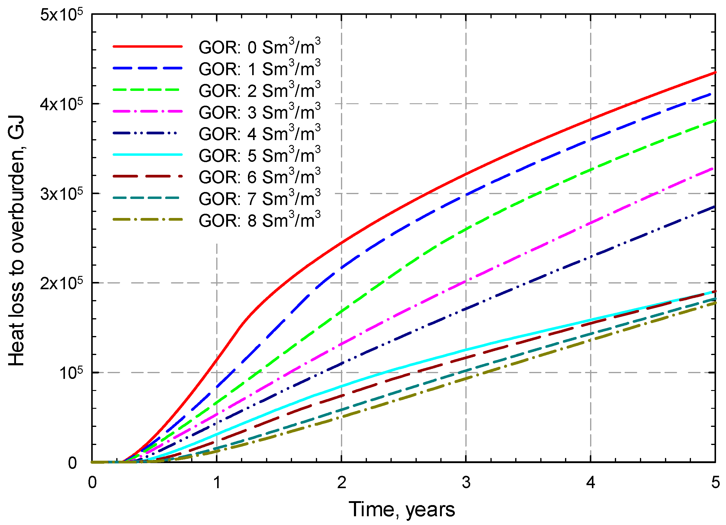
Figure 6.
Comparison of the oil recovery factor (RF) with different initial gas oil ratio (GOR) in the reservoir ranging from 0 to 8 Sm3/m3.
Figure 6.
Comparison of the oil recovery factor (RF) with different initial gas oil ratio (GOR) in the reservoir ranging from 0 to 8 Sm3/m3.
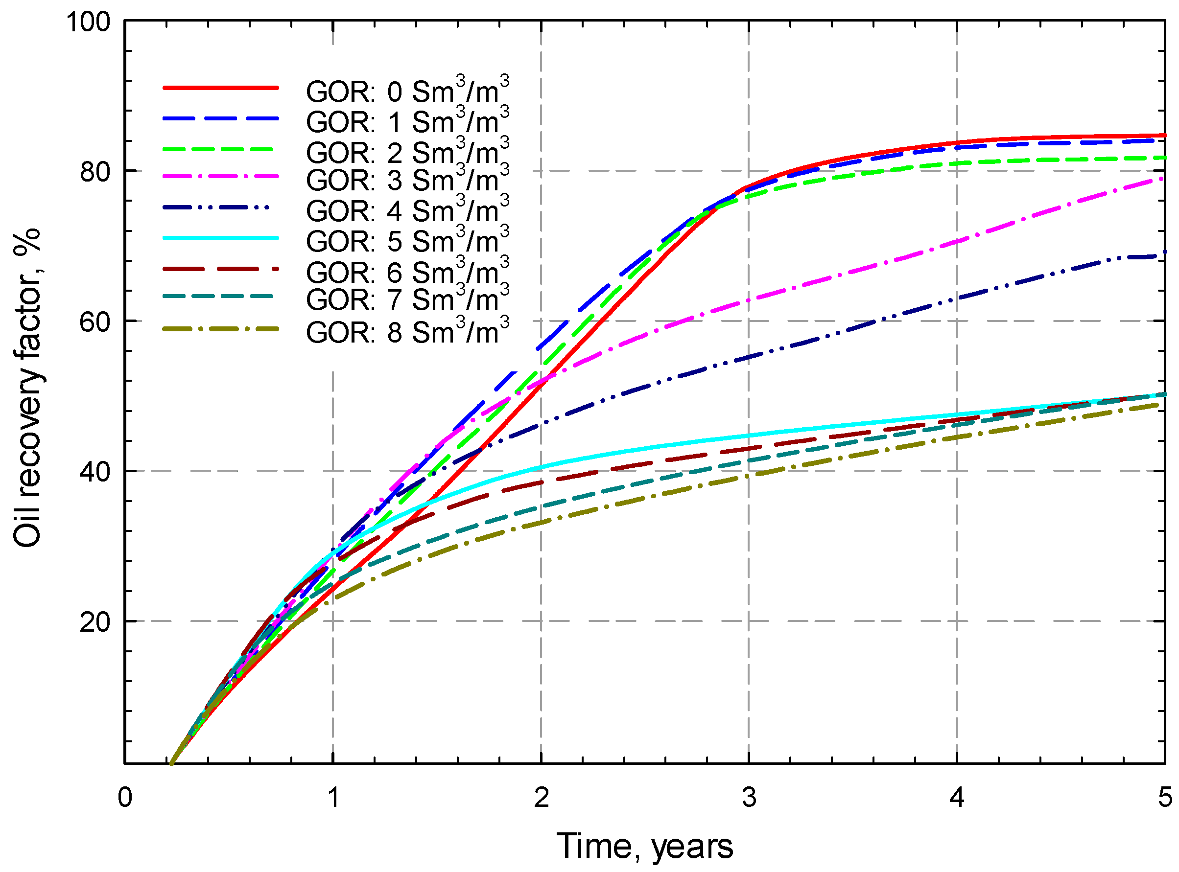
Figure 7.
Simulation results and correction curves for the defined factor (Y), the water production ratio from the bottom water zone (Rbw), and the volume of water produced from the bottom water zone (Qbw) under different thicknesses of the bottom water zone (hbw).
Figure 7.
Simulation results and correction curves for the defined factor (Y), the water production ratio from the bottom water zone (Rbw), and the volume of water produced from the bottom water zone (Qbw) under different thicknesses of the bottom water zone (hbw).
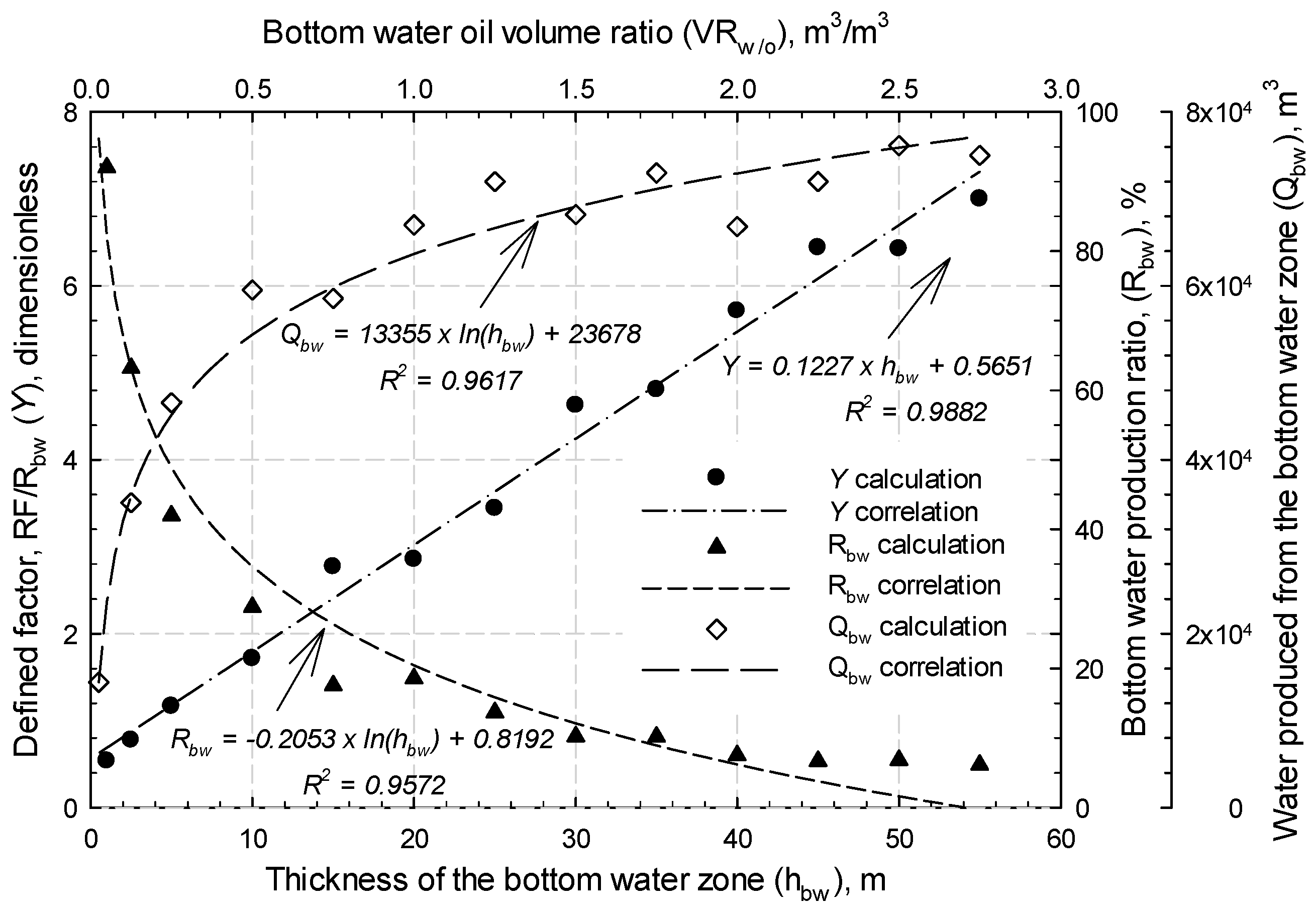
Figure 8.
The oil recovery factor and cumulative energy injected into the reservoir under different thicknesses of the bottom water zone.
Figure 8.
The oil recovery factor and cumulative energy injected into the reservoir under different thicknesses of the bottom water zone.

Figure 9.
Temperature distribution and water flow direction in the reservoir after 5 years of production: (a) reservoir without a bottom water zone and (b) reservoir with a 5-m bottom water zone.
Figure 9.
Temperature distribution and water flow direction in the reservoir after 5 years of production: (a) reservoir without a bottom water zone and (b) reservoir with a 5-m bottom water zone.

Figure 10.
Mole density of the gas phase in the reservoir after 5 years of production: (a) no oil in the bottom water zone; (b) 10% oil saturation in the bottom water zone; and (c) 50% oil saturation in the bottom water zone.
Figure 10.
Mole density of the gas phase in the reservoir after 5 years of production: (a) no oil in the bottom water zone; (b) 10% oil saturation in the bottom water zone; and (c) 50% oil saturation in the bottom water zone.

Figure 11.
Bottom water production ratio (Rbw) and oil recovery factor (RF) under different well pair locations.
Figure 11.
Bottom water production ratio (Rbw) and oil recovery factor (RF) under different well pair locations.

Figure 12.
Well pattern structures for (a) two corner wells in the I-K direction cross-section; (b) triple wells in the I-K direction cross-section; (c) DWS in the I-K direction cross-section; (d) VInj-HPro, and (e) fishbone well in the I-J direction cross-section.
Figure 12.
Well pattern structures for (a) two corner wells in the I-K direction cross-section; (b) triple wells in the I-K direction cross-section; (c) DWS in the I-K direction cross-section; (d) VInj-HPro, and (e) fishbone well in the I-J direction cross-section.

Figure 13.
Oil recovery factors of different well patterns applied in the reservoir with a bottom water zone, including two corner wells, triple wells, downhole water sink well (DWS), vertical injectors with horizontal producer (VInj-HPro), and fishbone well.
Figure 13.
Oil recovery factors of different well patterns applied in the reservoir with a bottom water zone, including two corner wells, triple wells, downhole water sink well (DWS), vertical injectors with horizontal producer (VInj-HPro), and fishbone well.

Figure 14.
Oil saturation distribution (in the I-K direction cross-section) of (1) two corner wells, (2) triple wells, and (3) fishbone well at the end of different production times: (a) 0.5 years; (b) 1 year; (c) 2 years; and (d) 5 years.
Figure 14.
Oil saturation distribution (in the I-K direction cross-section) of (1) two corner wells, (2) triple wells, and (3) fishbone well at the end of different production times: (a) 0.5 years; (b) 1 year; (c) 2 years; and (d) 5 years.

Figure 15.
Water cut for the cases with DWS under different pressure constraints in the DWS.
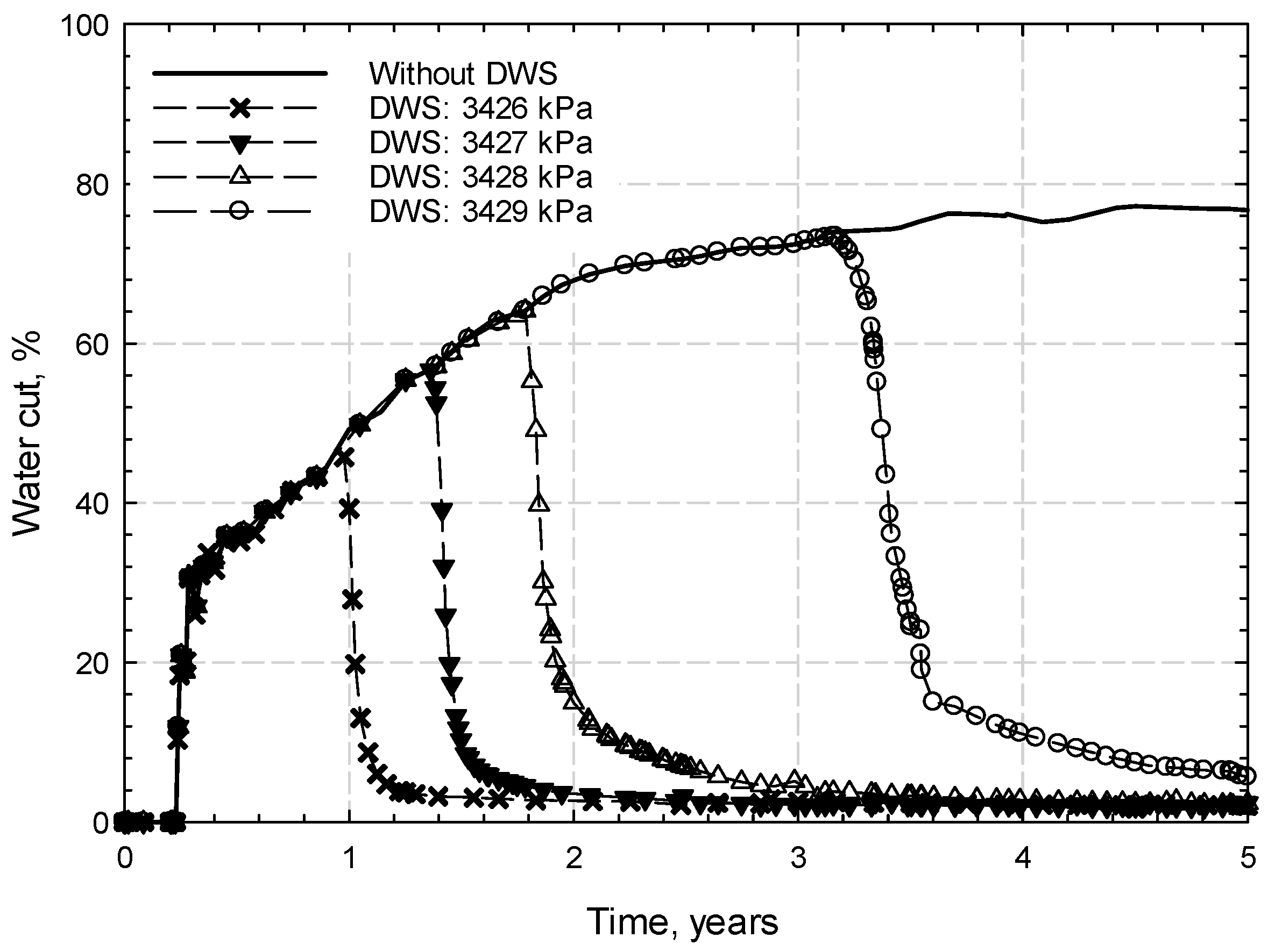
Figure 16.
Water flow direction near the wells for the DWS well pattern at a pressure constraint of 3428 kPa: (a) production after 1 year; (b) production after 2 years; (c) production after 3 years; and (d) production after 5 years.
Figure 16.
Water flow direction near the wells for the DWS well pattern at a pressure constraint of 3428 kPa: (a) production after 1 year; (b) production after 2 years; (c) production after 3 years; and (d) production after 5 years.

Figure 17.
Oil distribution in the reservoir at the end of five years of production in the VInj-HPro well pattern.
Figure 17.
Oil distribution in the reservoir at the end of five years of production in the VInj-HPro well pattern.


Table 1.
Properties of the reservoir in the Pikes Peak oil field, Lloydminster region.
| Parameter | Value |
|---|---|
| Depth (m) a | 500 |
| Initial reservoir temperature (°C) a | 18 |
| Initial reservoir pressure (kPa) b | 3350 |
| Thickness of oil zone (m) a | 20 |
| Porosity a | 0.34 |
| Permeability in the oil zone (mD) a | 5000 |
| Permeability in the bottom water zone (mD) a | 2000 |
| Oil saturation a | 0.85 |
| Formation compressibility (1/kPa) c | 2.0 × 10⁻⁶ |
| Rock, over-/underburden heat capacity J/(m3·°C) d | 2.39 × 10⁶ |
| Rock, over-/underburden thermal conductivity J/(m3·°C) d | 2.333 × 10⁵ |
| Oil phase thermal conductivity J/(m3·°C) d | 2.0 × 10⁴ |
| Water thermal conductivity J/(m3·°C) d | 5.35 × 10⁴ |
| Method for evaluation of 3-phase Kro e | Stone’s second model |
| Methane K-value correlation e K = (KV1/P) × EXP((KV4)/(T−KV5)) | |
| KV1 (kPa) e | 5.4547 × 10⁵ |
| KV4 (°C) e | −879.84 |
| KV5 (°C) e | −265.99 |
Table 2.
Properties of the oil sample applied in this study.
| Properties | Value |
|---|---|
| Density @18·°C (kg/m3) a | 985 |
| API gravity a | 12.4 |
| Viscosity @ 18·°C (mPa·s) a | 25,000 |
| Oil formation volume factor (m3/m3) a | 1.022 |
| Initial solution GOR (Sm3/m3) b | 8.0 |
| SARA composition (wt%) c | |
| Saturates | 23.1 |
| Aromatics | 41.7 |
| Resins | 19.5 |
| Asphaltenes | 15.3 |
| Solids | 0.4 |
Table 3.
Relative permeability applied in this study [41].
Table 3.
Relative permeability applied in this study [41].
| Water-Oil Relative Permeability | Liquid-Gas Relative Permeability | ||||
|---|---|---|---|---|---|
| Sw | Krw | Krow | Sl | Krg | Krog |
| 0.150 | 0.000 | 1.000 | 0.150 | 1.000 | 0.000 |
| 0.200 | 0.000 | 0.981 | 0.200 | 0.950 | 0.000 |
| 0.250 | 0.005 | 0.955 | 0.250 | 0.844 | 0.005 |
| 0.300 | 0.008 | 0.723 | 0.300 | 0.724 | 0.008 |
| 0.350 | 0.013 | 0.602 | 0.350 | 0.603 | 0.018 |
| 0.400 | 0.025 | 0.472 | 0.400 | 0.471 | 0.027 |
| 0.450 | 0.042 | 0.351 | 0.450 | 0.353 | 0.047 |
| 0.500 | 0.069 | 0.243 | 0.500 | 0.240 | 0.069 |
| 0.550 | 0.103 | 0.166 | 0.550 | 0.168 | 0.107 |
| 0.600 | 0.149 | 0.110 | 0.600 | 0.095 | 0.156 |
| 0.650 | 0.207 | 0.072 | 0.650 | 0.079 | 0.209 |
| 0.700 | 0.275 | 0.040 | 0.700 | 0.047 | 0.274 |
| 0.750 | 0.354 | 0.016 | 0.750 | 0.033 | 0.354 |
| 0.800 | 0.449 | 0.000 | 0.800 | 0.024 | 0.450 |
| 0.850 | 0.565 | 0.000 | 0.850 | 0.014 | 0.564 |
| 0.900 | 0.693 | 0.000 | 0.900 | 0.009 | 0.689 |
| 0.950 | 0.838 | 0.000 | 0.950 | 0.005 | 0.838 |
| 1.000 | 1.000 | 0.000 | 1.000 | 0.000 | 1.000 |
Sw: water phase saturation; Krw: relative permeability of water phase in the water-oil table; Krow: relative oil phase permeability in the water-oil table; Sl: liquid phase saturation; Krg: relative gas phase permeability in the liquid-gas table; Krog: relative oil phase permeability in the liquid-gas table.
Table 4.
Simulation results for different oil saturations in the bottom water zone.
| So,bw | OOIP | Rinc,OOIP | Rbw | Rinc,Rbw | RF | Rinc,RF | cEOR | Rinc,cEOR |
|---|---|---|---|---|---|---|---|---|
| % | 105 m3 | % | % | % | % | % | GJ/m3 | % |
| 0 | 3.775 | - | 41.953 | - | 48.972 | - | 4.062 | - |
| 10 | 3.886 | 2.943 | 46.462 | 10.748 | 49.250 | 0.568 | 3.994 | −1.671 |
| 20 | 3.997 | 5.884 | 45.557 | 8.591 | 49.024 | 0.107 | 3.912 | −3.682 |
| 30 | 4.108 | 8.827 | 45.242 | 7.838 | 49.581 | 1.245 | 3.752 | −7.627 |
| 40 | 4.219 | 11.768 | 43.274 | 3.149 | 45.886 | −6.301 | 3.624 | −10.782 |
| 50 | 4.330 | 14.711 | 37.311 | −11.066 | 43.282 | −11.619 | 3.325 | −18.128 |
So,bw: oil saturation in the bottom water zone; OOIP: original oil in place; Rinc,OOIP: incremental of the OOIP compared with the base case; Rbw: water production ratio in the bottom water zone; Rinc,Rbw: incremental of the Rbw compared with the base case; RF: oil recovery factor; Rinc,RF: incremental of the oil recovery factor compared with the base case; cEOR: cumulative energy oil ratio; Rinc,cEOR: incremental of the cEOR compared with the base case.
© 2017 by the authors. Licensee MDPI, Basel, Switzerland. This article is an open access article distributed under the terms and conditions of the Creative Commons Attribution (CC BY) license (http://creativecommons.org/licenses/by/4.0/).
Share and Cite
MDPI and ACS Style
Ni, J.; Zhou, X.; Yuan, Q.; Lu, X.; Zeng, F.; Wu, K. Numerical Simulation Study on Steam-Assisted Gravity Drainage Performance in a Heavy Oil Reservoir with a Bottom Water Zone. Energies 2017, 10, 1999. https://doi.org/10.3390/en10121999
AMA Style
Ni J, Zhou X, Yuan Q, Lu X, Zeng F, Wu K. Numerical Simulation Study on Steam-Assisted Gravity Drainage Performance in a Heavy Oil Reservoir with a Bottom Water Zone. Energies. 2017; 10(12):1999. https://doi.org/10.3390/en10121999
Chicago/Turabian StyleNi, Jun, Xiang Zhou, Qingwang Yuan, Xinqian Lu, Fanhua Zeng, and Keliu Wu. 2017. "Numerical Simulation Study on Steam-Assisted Gravity Drainage Performance in a Heavy Oil Reservoir with a Bottom Water Zone" Energies 10, no. 12: 1999. https://doi.org/10.3390/en10121999
Note that from the first issue of 2016, this journal uses article numbers instead of page numbers. See further details here.