Solution Validation for a Double Façade Prototype

Abstract

A Solution Validation involves comparing the data obtained from the system that are implemented following the model recommendations, as well as the model results. This paper presents a Solution Validation that has been performed with the aim of certifying that a set of computer-optimized designs, for a double façade, are consistent with reality. To validate the results obtained through simulation models, based on dynamic thermal calculation and using Computational Fluid Dynamic techniques, a comparison with the data obtained by monitoring a real implemented prototype has been carried out. The new validated model can be used to describe the system thermal behavior in different climatic zones without having to build a new prototype. The good performance of the proposed double façade solution is confirmed since the validation assures there is a considerable energy saving, preserving and even improving interior comfort. This work shows all the processes in the Solution Validation depicting some of the problems we faced and represents an example of this kind of validation that often is not considered in a simulation project.

1. Introduction

In the framework of the project JSEED [1,2], a set of experiments are conducted to obtain an optimal solution for a double façade prototype, with the aim of improving the building’s energy savings. In order to ensure that the correct decisions are made, a prototype that responds to the parameters selected was built. With this prototype, a comparison between the models and the data that we obtain for the prototype was performed. This allows validation of the methodology and the hypotheses in order to reuse the models in other climatic areas or with other parameters, avoiding the need to build new prototypes. This experience depicts a complete system validation and explains the methodologies used in the development of the project.

The Validation and the Verification of a simulation model are key elements to increase the model confidence [3]. Several techniques can be applied [4,5], and some recommendations can be followed [6]. A conceptual model can help in this process, becoming a central factor to perform this validation [4,7]. An example that takes advantage of the power of formal languages to perform the validation of the model can be reviewed in [8], where UML is combined with Petri nets (a formal and unambiguous formalism) in order to define test scenarios to be applied in the simulator. In our approach, we are taking the advantage of formal languages, using Specification and Description Language (SDL) [9] to represent the model allowing an automatic implementation of it, simplifying the verification process. The validation process was done, reviewing with the specialist the model (model validation) and performing a black and white box validation. In this formal representation of the system, all the hypotheses that must be tested are described. With the first executions of the model, different tests can be performed, comparing the results with the existing system, if it exists, or, with similar systems or the knowledge that the specialist has, if the system does not exist. To ensure that a simulation model is accurate, Solution Validation must be applied, if possible. The Solution Validation process compares the final implementation (in the system, based on the model results) with the results obtained by the simulation model, “The aim of all modelling and V&V efforts is to try to assure the validity of the final solution; once implemented, it should be possible to validate the implementation against the model’s results” [10]. Solution validation assures that the hypotheses are correct and the hypotheses proposed for the formal representation of the system (the model) are also correct and then, can be used on new scenarios with more confidence. Solution Validation is complex because as is stated in [11]: “solution validation can only take place post-implementation of the study’s findings”; also, specifically the validation of environmental models is a complex task due to the inherent complexity of the considered elements and the huge amount of data that are going to be used; see [12,13]. Because of this complexity, some work conducted validation analysis in the analysis and the classification of the input data; see [14], or in the sensitivity analysis of the model data; see [15]. But usually no validations are done implying the real system with the proposed modifications, i.e., the Solution Validation, that allows complete understanding if the assumptions are correct or not. The lack of this type of validation in this kind of system is obvious because of two aspects:

• This validation must be done once the simulation project is finished and once the implementation of the results obtained from the model are applied to the system. This implies that the contractor believes in the model, and now we are going to perform a new validation.
• The complexity to analyze the modified system in this ambit (environmental area).

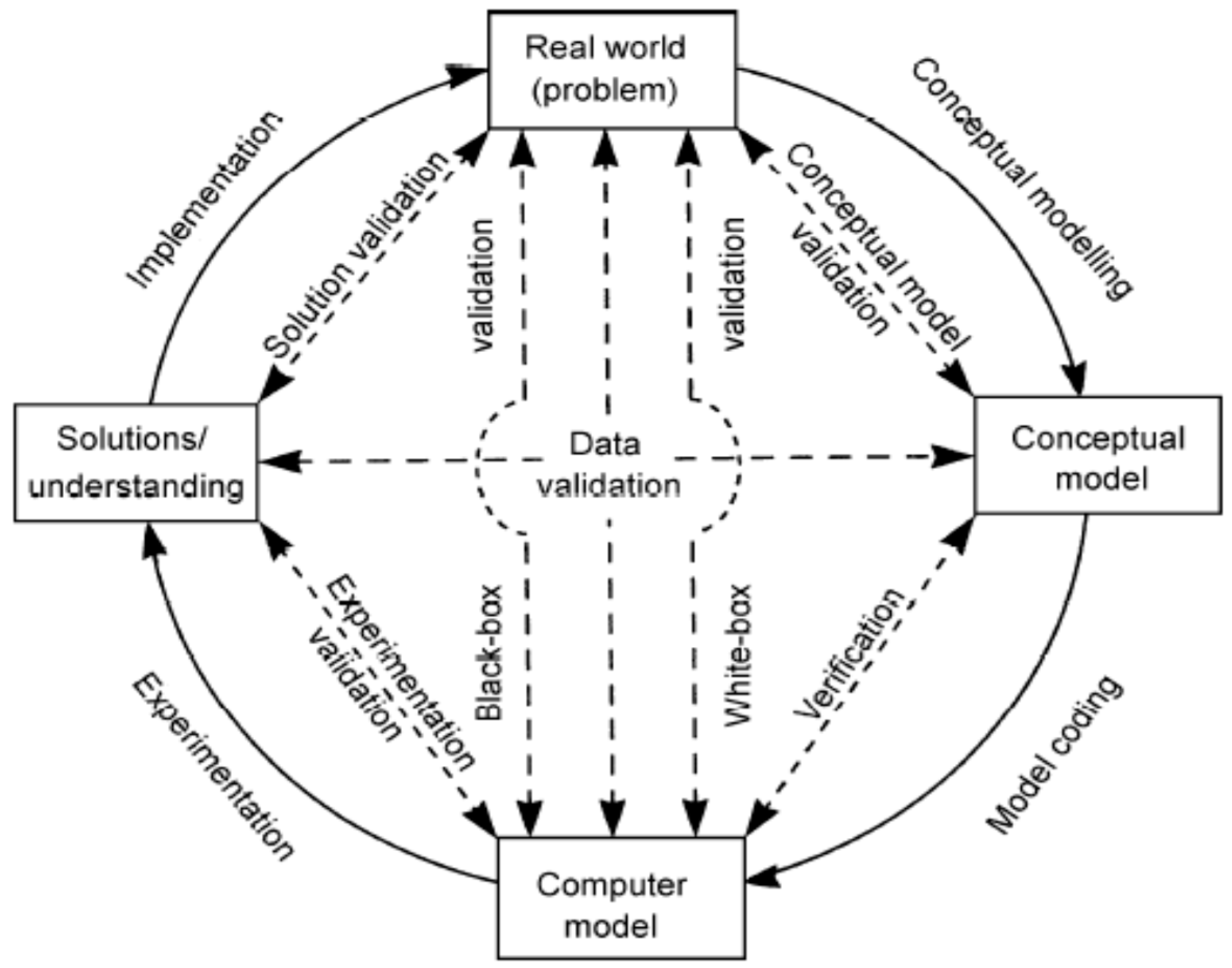
In this paper, we analyze the Solution Validation and the methodologies used in the whole development of the Validation Verification and Accreditation (VV & A) process; see Figure 1 to put this kin the context of a whole simulation project validation cycle. The model is focused on the analysis of the behavior of a building in order to improve its behavior, testing a new façade prototype. Studies that use simulation to analyze the behavior of ventilation exist and have become more and more common; see [16]. Here, we are going to be focused on the validation processes, specifically on system validation. This research area is intensively analyzed because buildings consume around 33% of energy worldwide; see [17]. This motivates an intensive research in this area, with an increasing applications of Operations Research techniques, to help in the design of environmental processes; see as examples [18,19,20,21,22,23,24,25,26]. Specifically, with respect buildings, without a calculus of their passive behavior, we cannot achieve a real improvement in the energy savings. The need to obtain the maximum benefit of solar and lighting in winter and heat protection in summer (mostly in temperate and not extreme climates) leads us to develop mixed solutions that enables adaptability depending on the time of year and climate zone. The premise of the project is to design a solution for building openings, mainly for office use, and focuses in different climatic zones of Spain. The project responds to the new European guidelines for energy savings, European directive 2010/31/EC [27] related to the energy efficiency of buildings and the data published by the International Energy Agency [28]. The need to propose solutions that help in the reduction of the energy demand in order to design buildings near NZEB [29,30] is an important premise to be considered in the design of a new prototype of building openings. In the project, a modular system composed by a double façade was developed. The main goal is to create an element that can be adapted easily to different buildings, that offers a good behavior from the point of view of the energy (passive and active), being transformed from a traditional window to a device that provides efficiency and comfort through a controlled operation.

In the project, we model and implement two prototypes and perform a complete solution validation to test if the proposed assumptions are correct. Solution validation needs a Verified, Validated and Accredited model to start. Those models are the ones that we are going to use to assure that all the whole process followed is correct, and to perform a new Accreditation for such models using a real system. To do so, we use black box validation techniques [11], where the results of the model will be compared with the data obtained for the system.

2. The Model

Major concerns in this kind of simulation are the climatic conditions to be used in the simulation model. In our case, we base this on [31]. Since the climatic zone selected is Seville, due to the situation of the Test Cell prototype, the IWEC database to be used will be Sevilla.epw based on the International Weather Climate [32].

Once the climatic conditions are fixed, the thermal comfort conditions need to be defined. To do so, the data provided by RD 1826/2009, published on the BOE of 11 December 2009 were used. These data supersede RITE (Reglamento de Instalaciones Térmicas de los Edificios), in the instruction RITE Section 3, and the RITE Section 4.

Table 1. Reference for the comfort data [33].

Offices	Temp. (°C)	% HR
Summer Inside	26	45–60
Winter Inside	21	40–50
Dwellings	Temp. (°C)	% HR
Summer Inside	25	50
Winter Inside	21	50

shows the references used for the comfort in this project.

Regarding the materials used in the definition of the simulation models, we always consider the prototype that will be constructed in order to simplify the solution validation, but without compromising the universality of the results that we can obtain. In that sense, although perimeter walls could have been simulated as adiabatic, we preferred to approximate the simulation model to the experimental study prototype. Thermal transmittance requirements for walls were 0.1 W/m²·K (30 cm thick rock wool); on the one hand, the resulting reference data (the data used to perform the comparison between the different simulations) do not increase significantly and, on the other hand, we prepare the virtual design with materials and their real properties.

Another important aspect to be considered is parameterization of the internal loads, the occupation and infiltration. To do so, we use the data provided by the IDAE and regulation of heating systems in buildings and the CTE [34]. To determine the infiltration, the data provided by the CTE were used, related to < 27 m³/h·m².

Another important aspect in the model is the glass materials to be used; see

Table 2. Glass materials used in the simulation models. Source [35].

Name Glass Material	Concept	Solar Transmission (SHGC)	U (W/m2·K)	Direct Solar Transmission	Light Transmission
FachTe_Glass_FV—SHGC 0.1, Light transmision 0.1, U 1.1	photovoltaic plate Schott	0.1	1.1	--	0.1
FachTe_Glass_6-8-6	double glass	0.5	3	0.373	0.5
FachTe_Glass_3-8-3	normal glass	0.828	3.087	0.813	0.839
FachTe_Glass_10-12-10	low-e glass	0.559	1.89	0.418	0.71
FachTe_Glass_6-13-6	solar control glass 6 + 12 + 6	0.168	1.672	0.087	0.114
FachTe_Glass_6	simple glass	0.819	5.718	0.775	0.881

.

The model incorporates not only the physical aspects needed to define the behavior of the building, but also the legislation, to assure the validity of the proposed solutions in the real context that we are facing.

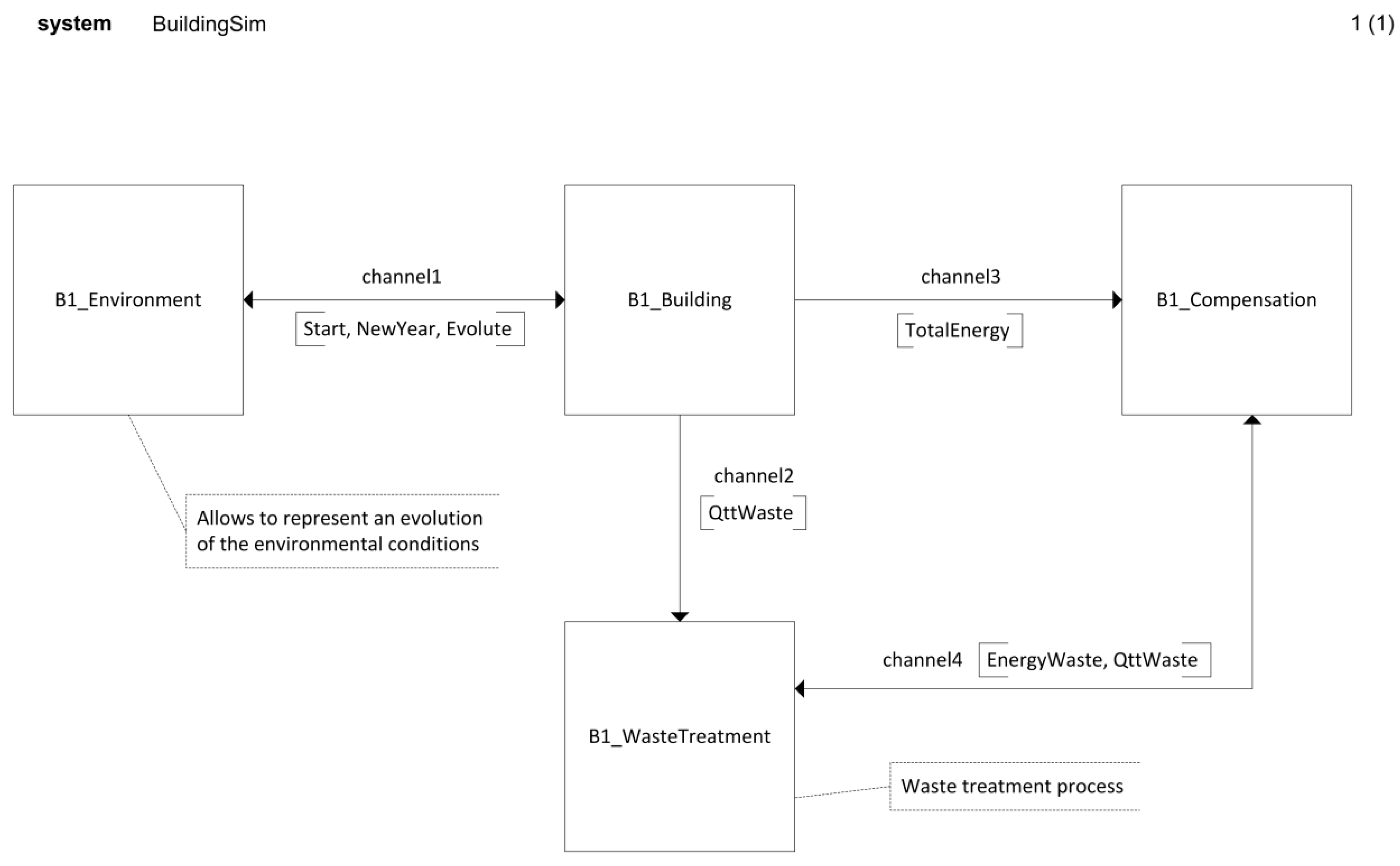
All these parameters, and the processes that rule the behavior of the building are defined using a formal representation based on Specification and Description Language formalism (SDL). In [36] you can review the details of the model used; in [37,38] an application of this methodology for the simulation analysis is shown. From this specification, a tool named SDLPS [39] allows the execution of the model formalized in SDL, obtaining the solutions without the need to perform a specific implementation. This simplifies the verification process.

The model is focused on analyzing the effects of the design elements over the energy consumption of the building. The proposed model allows us to find the optimal combination that satisfies the requirements and the needs of the design of a building, at both the environmental level and at the economic cost level. Figure 2 the system diagram that rules the behavior of our model is defined.

The model allows us to obtain comparative results, showing the effects of every constructive aspect regarding the total consumption of the building. Starting from there, the user can define different configurations for the design. In each configuration we can change the constructive solutions, the thickness of a wall, the orientation or the meteorology of the location of the building. The optimizer combines all the possible configurations to find a preferred optimal solution. In order to not reinvent the wheel, we use co-simulation techniques, using Energy Plus [40] as an energy consumption calculation engine.

Once the best desired configuration that responds to the objectives of the project is determined, CFD simulations were prepared (computational fluid dynamics software) to reach a more detailed proposal for the constructive solutions to be used (allowing an accurate control of the behavior of the proposed façade). CFD simulations allow analysis of the flows and the stratification of the resulting air, the behavior of the air heating, the façade materials thermal behavior and the space ventilation. 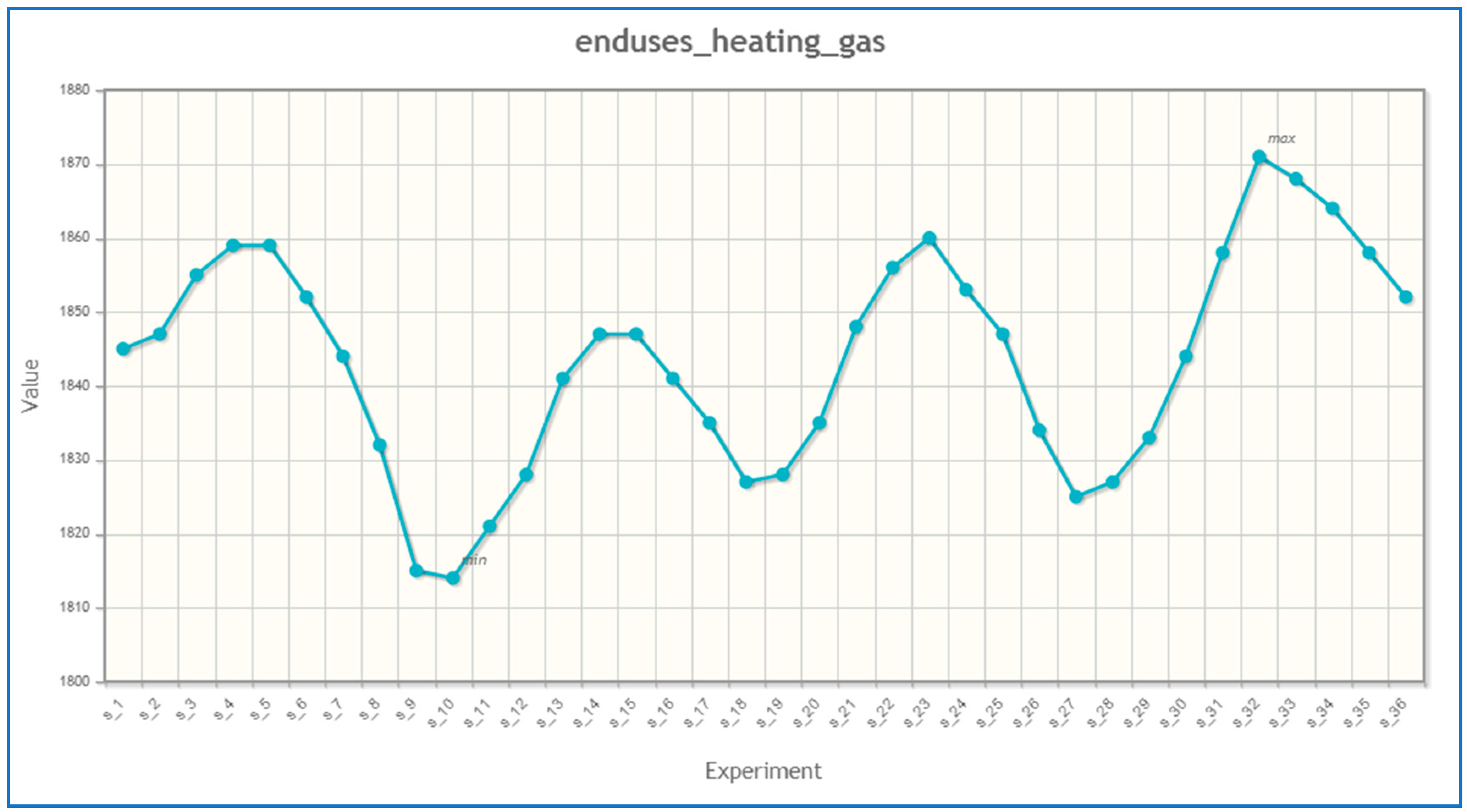Figure 3 shows energy consumption depending on the building orientation.

3. Implementing the Results in the System

The property, where the prototypes were built, belongs to ACCIONA Infraestructuras, S.L. The placement of prototypes did not present any difficulty, as the land was ready for it. In addition, there was no problem regarding shadows or strong winds.

Two prototypes were built in order to consider two main scenarios. The prototype is a block, similar to a building office, in Seville, south facing, for individual offices. The façade corresponding to the experimental prototype is 2 m × 2 m. The enclosure materials used in the prototype are shown in

Table 3. The enclosure materials used in the actual prototype.

Description	Materials (from Outside to Inside)	Thickness (cm)
Exterior	(sheet metal + camera air + battens) + insulation + pre-stressed wooden panel	0.3 + 5 + 8 + 10
Interior	Insulation + wood panel + finish	8 + 1.5 + 1.5
Ceiling	Sheet + camera air + insulation + waterproof sheet + panel wood freestanding	0.5 + 5 + 20 + 0.3 + 10
Door	Access for service space	--
Foundation	Wood base + wood leveling screed	variable

.

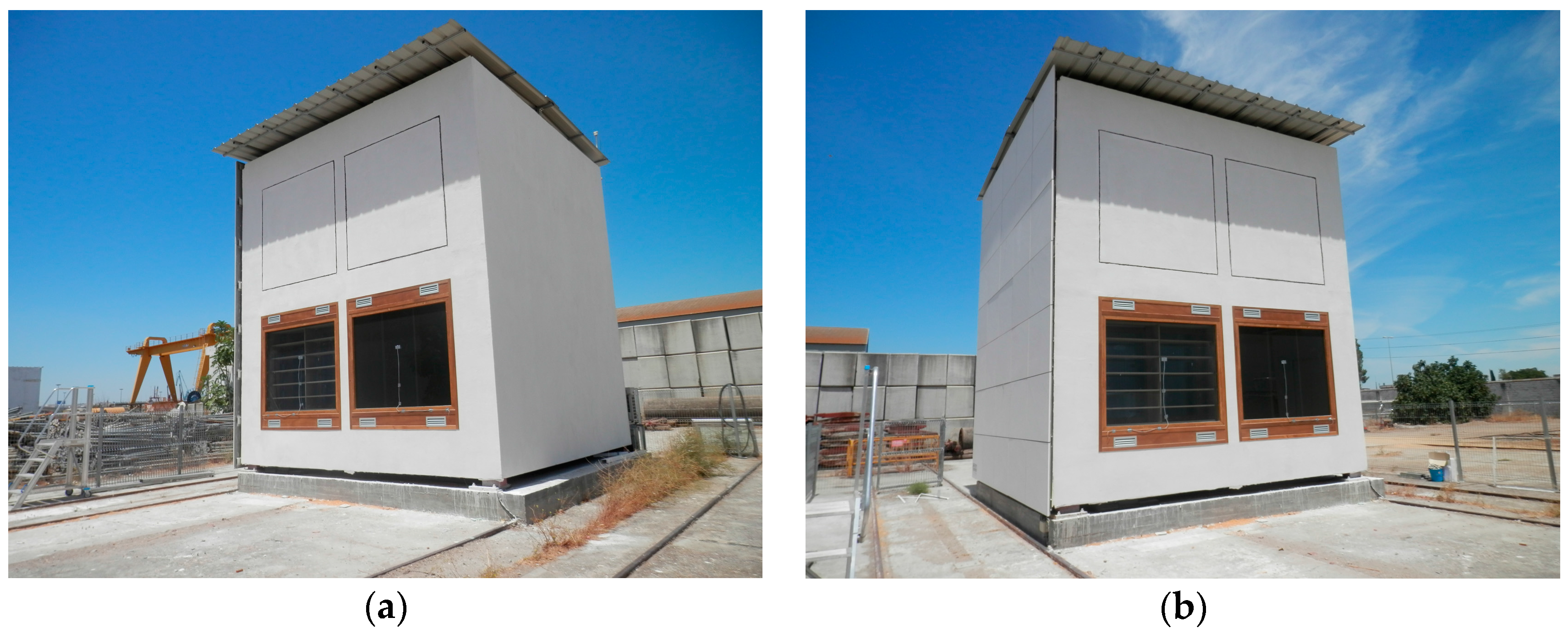
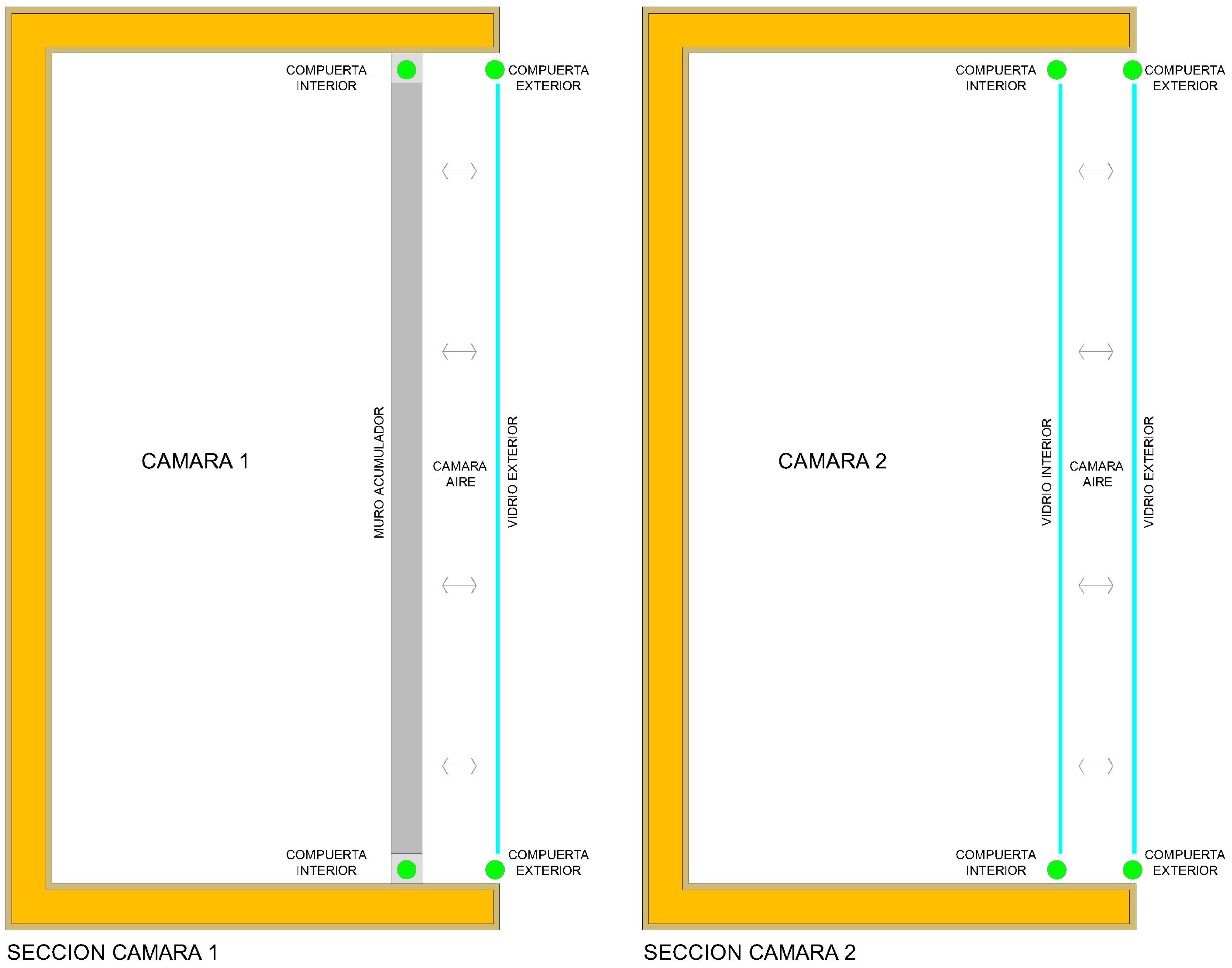
The first prototype is intended to be used to compare a double-glazed façade (glass + glass) with double glass + photovoltaic skin façade (see first floor of Figure 4). The second prototype, for the second façade, is composed by a climate system capable of allowing oscillations and thermal variations on the proposed air velocities. This second façade will be analyzed entirely in CFD; 8 scenarios will be executed (allowing the selection of 2 different airflows, 2 boundary conditions and 2 sizes of the air chamber). In this paper, the focus will be on this second prototype.

The prototype is separated from the terrain, about 30–50 cm, to avoid possible heat moisture or gas transfer. The effect on the thermal behavior of a space is very different depending on its contact (or not) with the ground, due to thermal inertia. Therefore, separating the prototype of the land is fundamental to make the correspondence between the model and the prototype as close as possible, especially when the prototype is only one height. Unions and joins have to be made through dry construction, following the pattern or models proposed by the Passivhaus standard certification, in such a way that the thermal bridges and discontinuities in the thermal insulation are avoided at all times.

3.1. Prototype Sensors

In order to enable the Solution Validation, information from the system must be obtained in real time. To do so, we add several sensors to the prototype to obtain mainly (i) the evolution of the average temperature of the airflow along the height of the cavity and (ii) a comparison, over time, of interior space against the outside ambient temperature. Next T Thermocouples were considered more appropriate, since they have a good sensibility, are resistant to oxidation, humidity and external agents, and cover the range of measurements which must be assured.

The distribution of the sensors was defined in order to capture temperature gradients and curves. Since in reality, important T gradients occur, it is not deemed representative to acquire only a value of T (since this varies greatly with the position). The sensors applied were to measure (i) Temperature and Humidity Relative (in the central section in different heights); (ii) superficial radiation, on envelope walls and the façade of the study; (iii) speed of the indoor air and (iv) illumination levels. We also measured the climatic changes on the outside of the prototype. Figure 5 shows the proposed sensor system distribution for the prototypes.

Wind speed needs to be measured. The distribution of anemometers consists of two vertical rows of sensors for each constructive configuration. This allows knowledge of the average speeds throughout the area. Again, only the value of air speed is not considered representative, since this variable depends on the place in which measurement is made.

The type of anemometer is the Omni-directional with hot foil, since the air direction is not known and it will change over time. These anemometers are insensitive to changes in the direction of the air, are the least influenced by temperature variations and can be easily attached to a data logger. In Figure 6, the anemometer distribution used for both prototypes is represented. The installation of a pyranometer to monitor the amount of radiation incident on the glass was also deemed important. This allows us to discard T increases/decreases due to a change in the amount of radiation (rather than because of the behavior of the prototype).

3.2. Data Acquisition

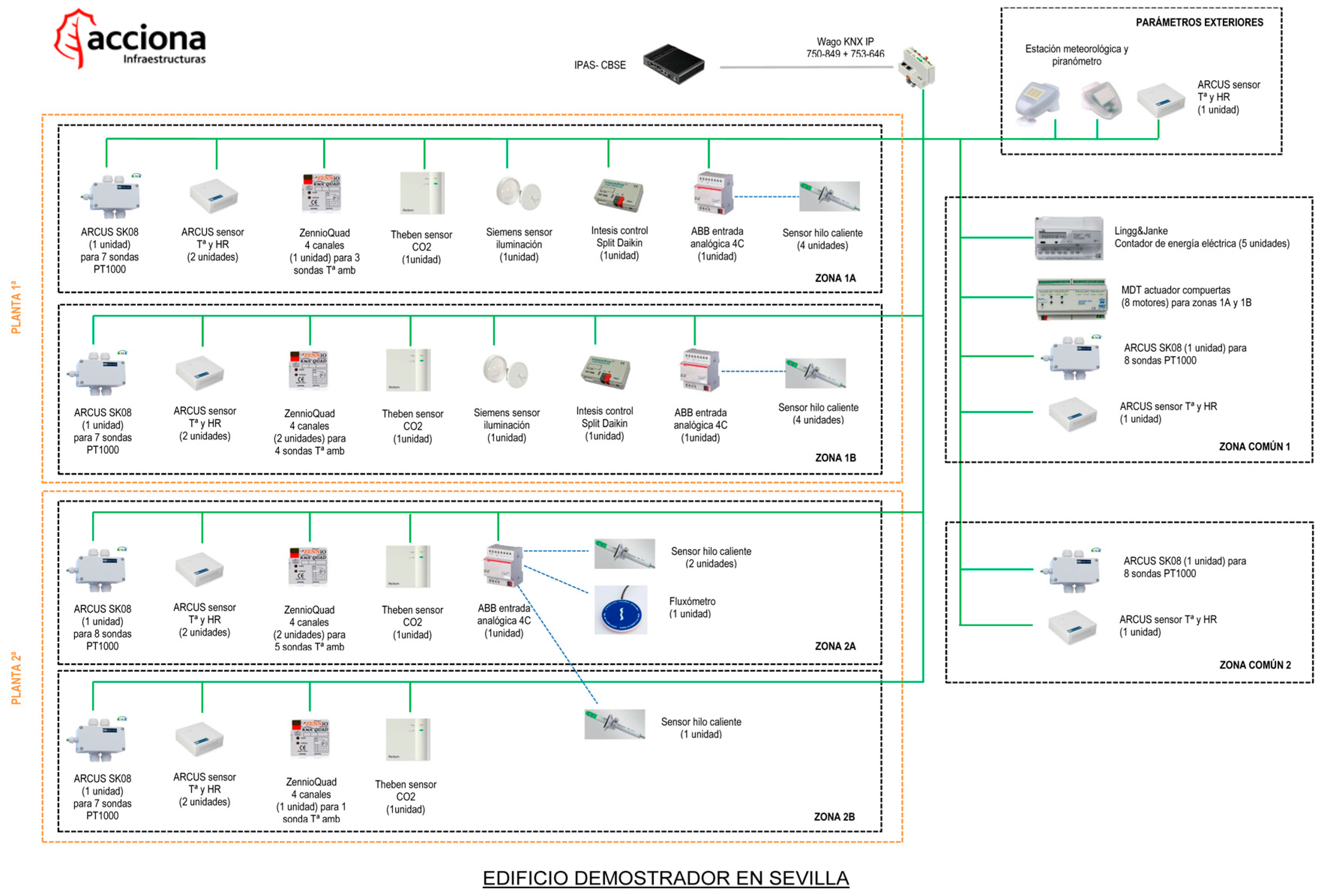
A unit is needed that registers and stores the signals coming from the sensors. This task can be accomplished in different ways depending on the number of channels and depending if continuous or punctual measures are required: from the use of simple multi-input Data Loggers to digital data acquisition units. 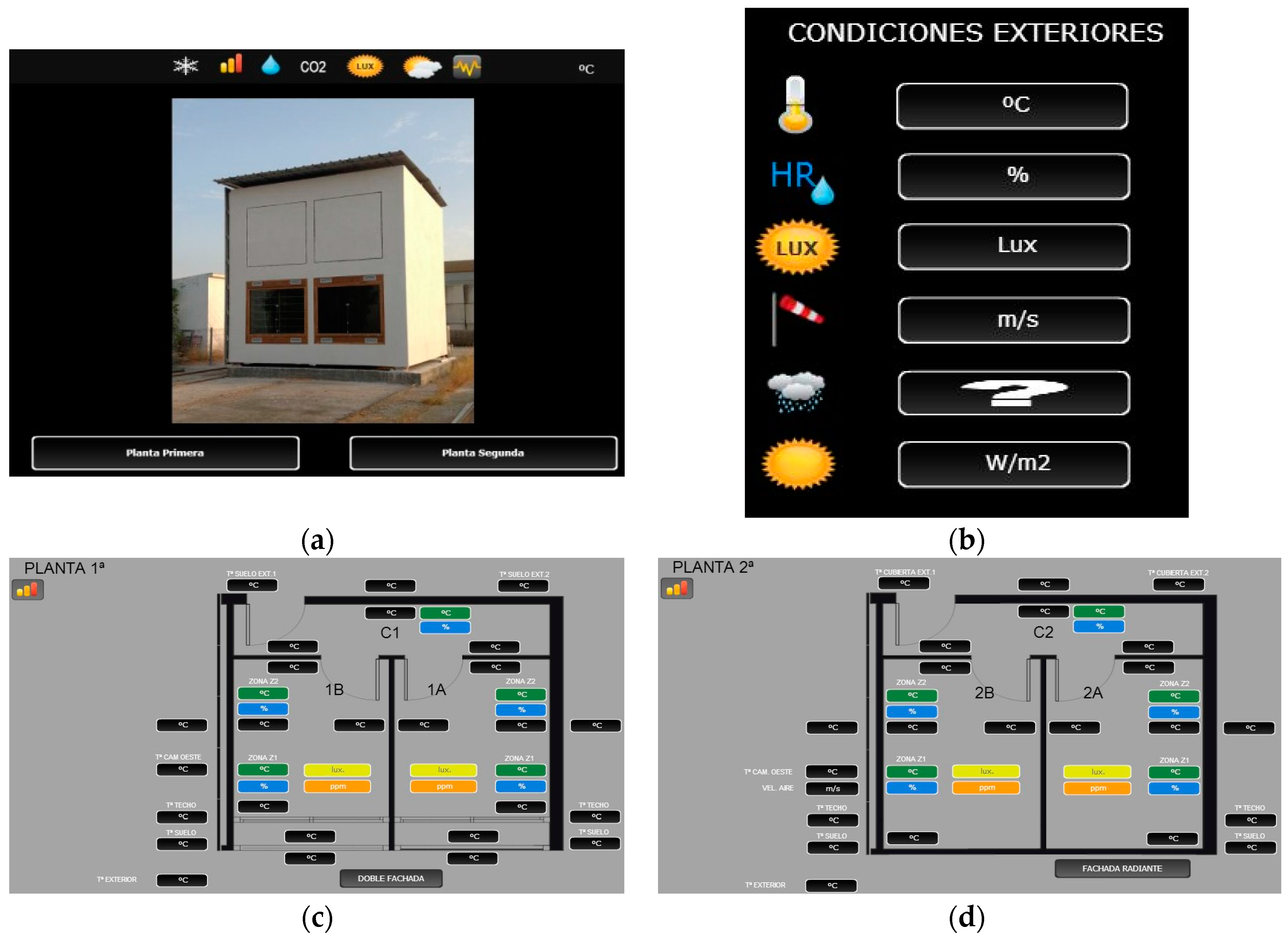Data obtained using the KNX system, developed by ACCIONA INFRAESTRUCTURAS were collected, see Figure 7. The monitored data were collected using the platform created by the group ACCIONA. The platform allows us to collect and export data using *.csv files for subsequent processing. The methodology used is as follows: export the needed data obtained from the different sensors, detect missing values (we found slots without data) and outliers and perform a post-processing analysis using statistical software. In Figure 8 the web monitoring system used to obtain the data is shown.

The external conditions to be analyzed are (i) temperature (°C); (ii) HR (%); (iii) Illumination (lux); (iv) Velocity (m/s), (v) Rainfall (mm/h) and (vi) Radiation (W/m²). The indoor conditions that can be analyzed and studied are (i) temperature (°C); (ii) HR (%); (iii) Illumination (lux); (iv) CO₂ (ppm); (v) Consumption (W) and (vi) Radiation (W/m²).

4. Solution Validation

This section checks the similarities or differences between the models and the real prototypes. Monitored months presented in the paper are from 15 August to 15 September.

Several techniques can be applied for the validation of the solution [3,6]. The Visual Inspection of the Data and Black Box Validation, applying a set of proposed statistical methods, have been depicted.

4.1. Visual Inspection of the Data

The purpose is to substantiate that the model correctly represents the behavior of the system, and detect when this representation is not accurate and why. Therefore, talking with the experts and detecting possible problems in the model, or in the sensors we used to obtain the data, is needed. This analysis is needed to detect any kind of interference of external elements with the sensors, a fact that implies the introduction of some extra noise in the records.

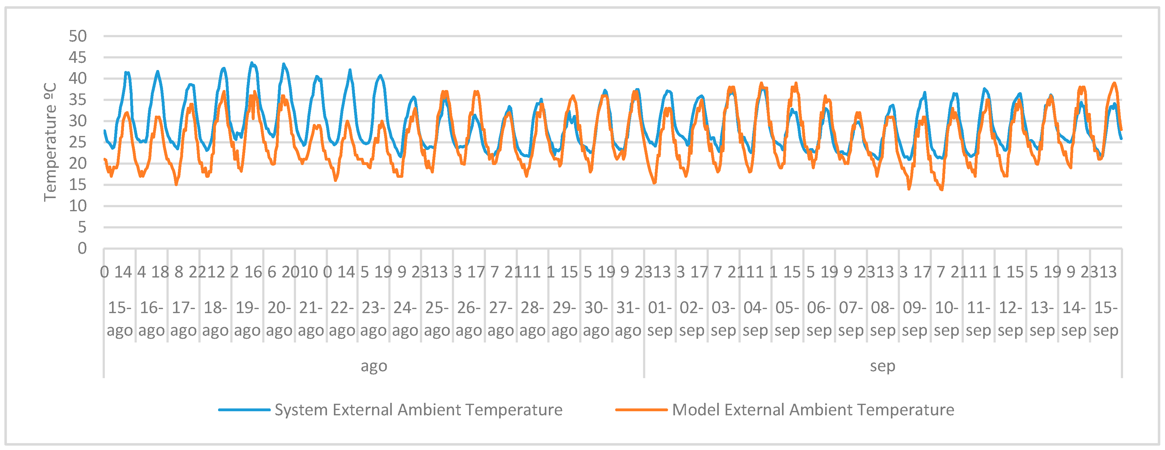
The first thing to be considered, for a correct comparison of results, is boundary conditions, temperature, humidity, etc. In this case, temperature and solar radiation data for the period studied were consulted. Figure 9 shows the comparison between the exterior temperature for the model and for the system. We can see that, although both charts follow the same pattern, a difference in the magnitude is clear in the first few days. The deviation regarding the mean minimum temperatures of the model implies a higher daily thermal jump in the model data, compared with the system data. A detailed analysis also allows us to detect that until 21 August, the temperatures in the system were very high (compared to those obtained from the model), we discuss this later in the statistical analysis.

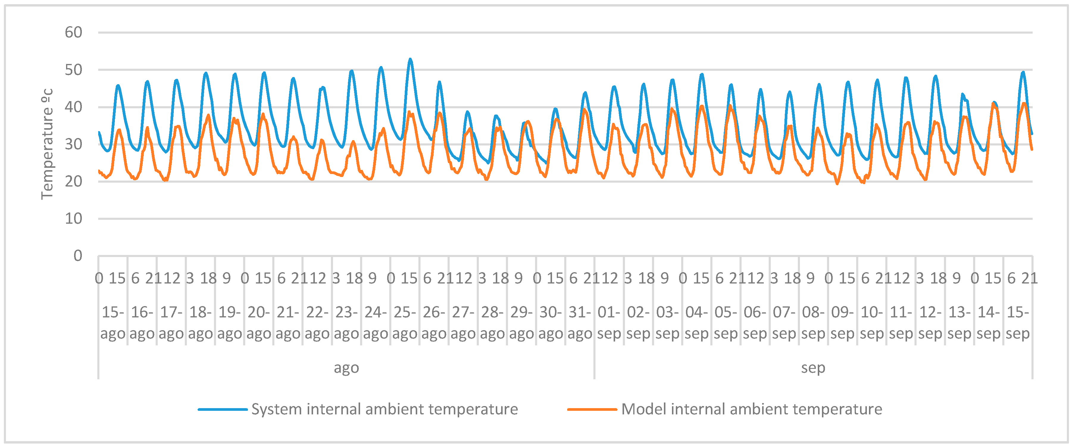
The internal temperature depends on the external temperature and the behavior of the system (ambient temperature). Figure 10 shows the chart that depicts the comparison between the obtained data from the system and the model regarding the internal building temperature.

These differences are around 10 °C and may be due to the different boundary conditions (temperature outside the system) or, with greater probable incidence, that the model defines a bigger ventilation feedback in the chamber. Here, a deeper analysis to conclude what fails is needed. This is clearly related to the external temperature as it was detected previously. Our Model assumes a normal summer, fact that is not true for the summer of 2013 in Seville.

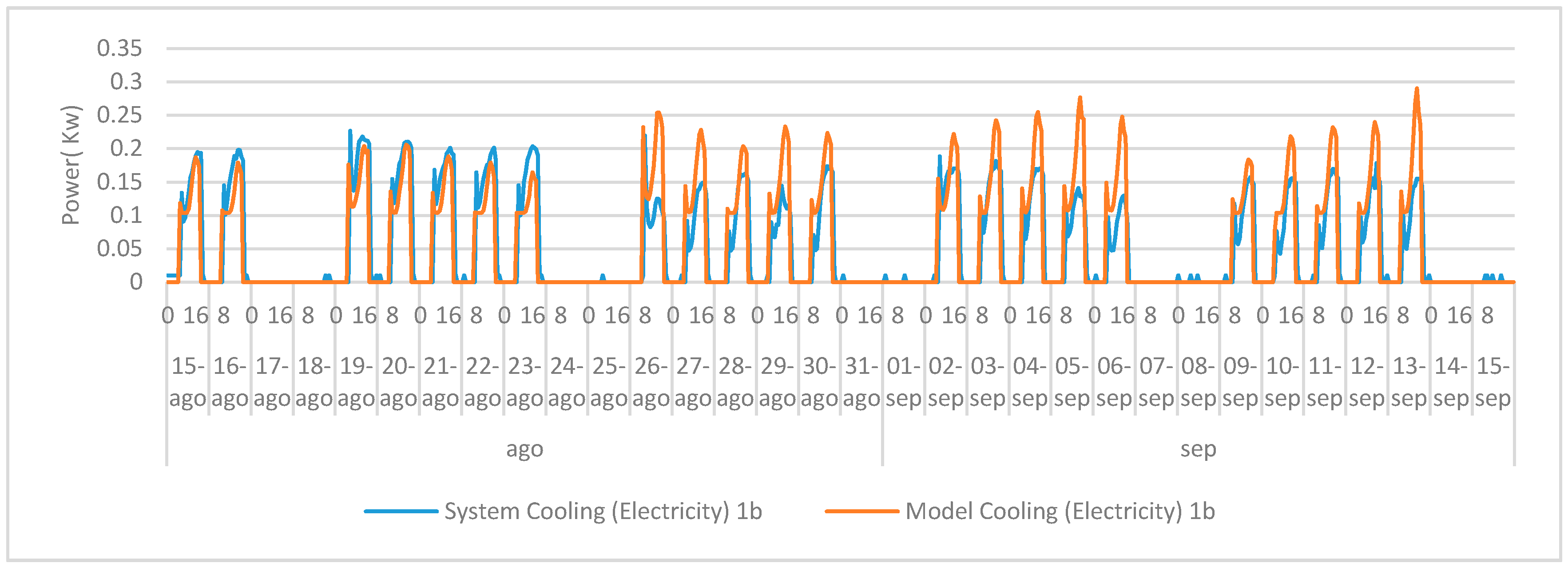
Another interesting element to consider is the acclimatization system. In Figure 11 the behavior of the cooling acclimatization system (analyzing the kW) for the model and the system is represented. It can be seen that in the first 7 days there is a remarkable coincidence of power consumption between model and system. In the next three weeks, these values indicate a greater difference. It would be interesting to perform a study across the values of other variables, over the same period, to determine whether there is any explanation for this divergence.

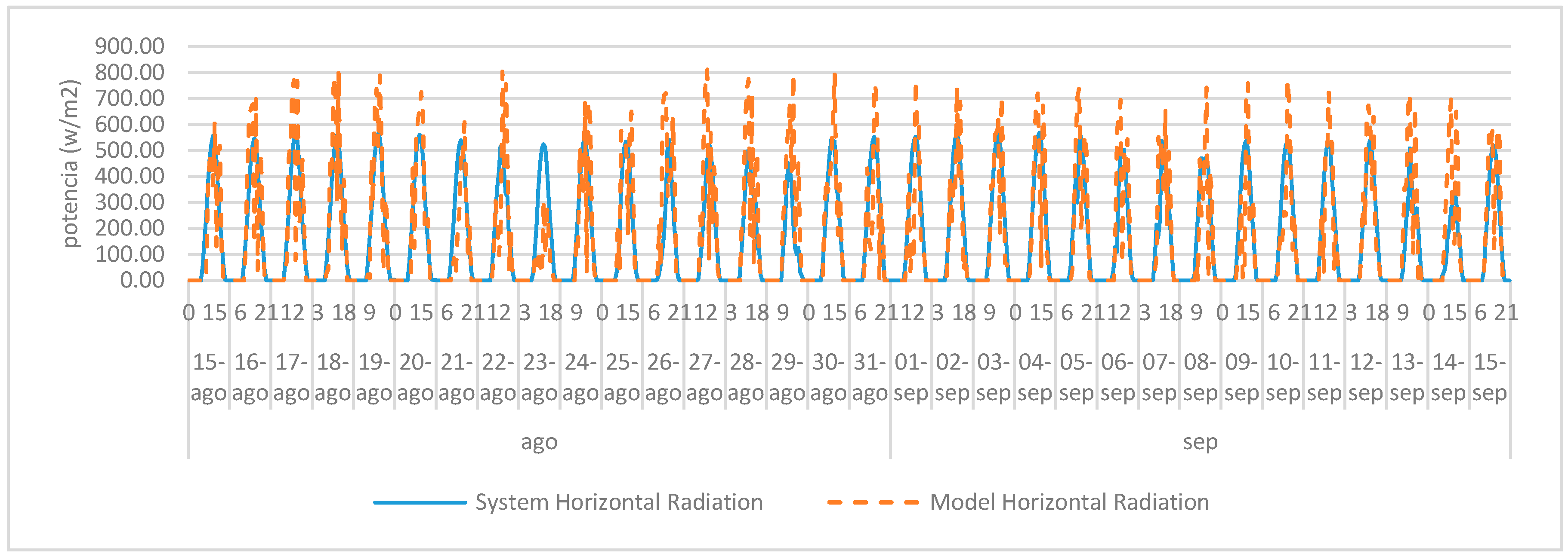
Regarding the horizontal radiation values for the system, they seem to be around 20% lower than those values obtained from the model. Despite the fact that there is this deviation in terms of magnitude, the fact that it is fairly homogeneous allows us to conclude that the model is accurate enough for use.

All of this graphical information and the first analysis done using the information of the experts, on both the model and the system, lead us to suggest some modifications in the model (some calibrations) and other modification on the sensors that allows us to obtain the information of the system (similar to the case of the outdoor temperature).

Other techniques can be applied here, like statistical techniques in order to understand the level of correctness to conclude, from a statistical point of view, that the model is valid.

4.2. Statistical Analysis of the Solution

To perform a Solution Validation, a Black Box technique can be used [4]. With this technique it is assumed that nothing is known regarding the model. Mainly the inner idea is to analyze the obtained data and compare them with the data we obtain from the system. We are focused here on the analysis of the radiation, the external and the internal temperature since these three cases present different levels of complexity regarding the validation. We are working on all tests at 95%.

4.2.1. Radiation

We start working with Radiation, see Figure 12, obtaining the mean for every day and analyzing if the measurements we obtain in the system are equivalent to the results we previously obtained with the simulator. Applying a common Wilcoxon test [41] (we cannot assume normality of the radiation observations over time; hence, we cannot apply a paired t-test), we cannot discard the null hypotheses; hence, we can argue that both samples belong to the same population (p-value is > 0.05). The solution to the tests is presented here using R statistical language. We compare the radiation information for the model with the data we obtained from the system.

• Wilcoxon signed rank test
• data: Data.for.the.paper.by.day$Radiation_model and Data.for.the.paper.by.day$Radiation_system.
• V = 326, p-value = 0.2539
• Alternative hypothesis: true location shift is not equal to 0

If all the time series are analyzed, not just the mean, the obtained values support again that the null hypotheses cannot be discarded.

• Wilcoxon signed rank test with continuity correction
• data: Data.for.the.paper$Radiation_model and Data.for.the.paper$Radiation_system
• V = 49500.5, p-value = 0.292
• Alternative hypothesis: true location shift is not equal to 0

In the case of radiation, the simulator patterns fit well with the pattern of the data obtained with the system, and the statistical test confirms this. Hence, it can be assumed that the simulator behaves as expected and (most important) the sensors are correctly placed.

4.2.2. External Temperature

The next step is to review what happens with the temperature variable. First, a comparison using the Wilcoxon test is done. In this case, analyzing the mean for every day, and comparing the results obtained from the model and the system, it is concluded that null hypotheses must be rejected.

• Wilcoxon signed rank test
• data: Data.for.the.paper.by.day$Temperature_model and Data.for.the.paper.by.day$Temperature_system
• V = 52, p-value = 1.802 × 10⁻⁵
• alternative hypothesis: true location shift is not equal to 0

Hence, in the case of temperature, we cannot conclude that the model fits well with the data.

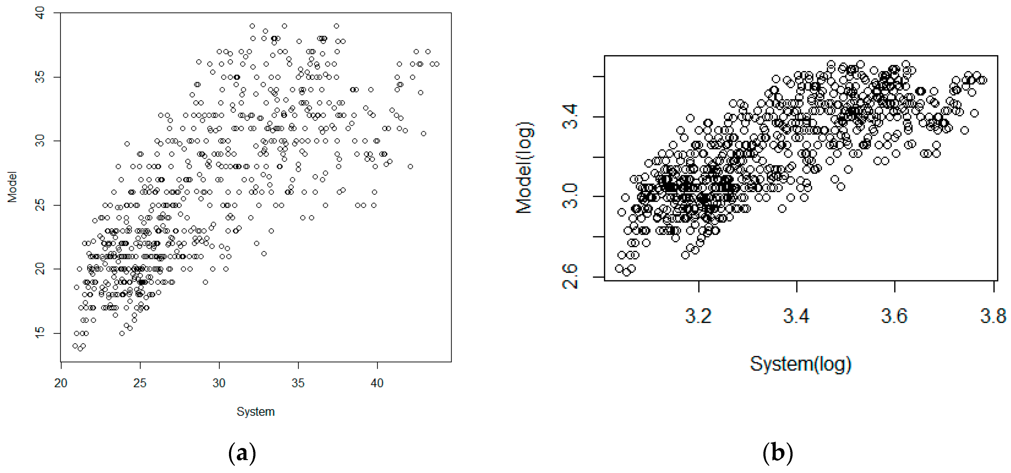
We can validate this (we do so) using historical data, but this is not the kind of validation we are presenting here. A Solution Validation must include the data we obtain from the system, to detect possible problems related to the data acquisition, implementation of the solutions or (as the last alternative) the model assumptions. As an initial step, we draw a chart, see Figure 13a, depicting the relation between the system and model temperatures. Analyzing the patterns, a logarithmic transformation of the data can help to smooth the relation between both variables; by doing so, the chart represented in Figure 13b has been obtained.

Now, the represented data can be analyzed by logarithmic transformation. This analysis indicates that the data obtained from the model do not correctly fit the data obtained from the system.

• Wilcoxon signed rank test
• data:Data.for.the.paper.by.day$Temperature_model_log and Data.for.the.paper.by.day$Temperature_system_log
• V = 51, p-value = 1.603 × 10⁻⁵
• alternative hypothesis: true location shift is not equal to 0

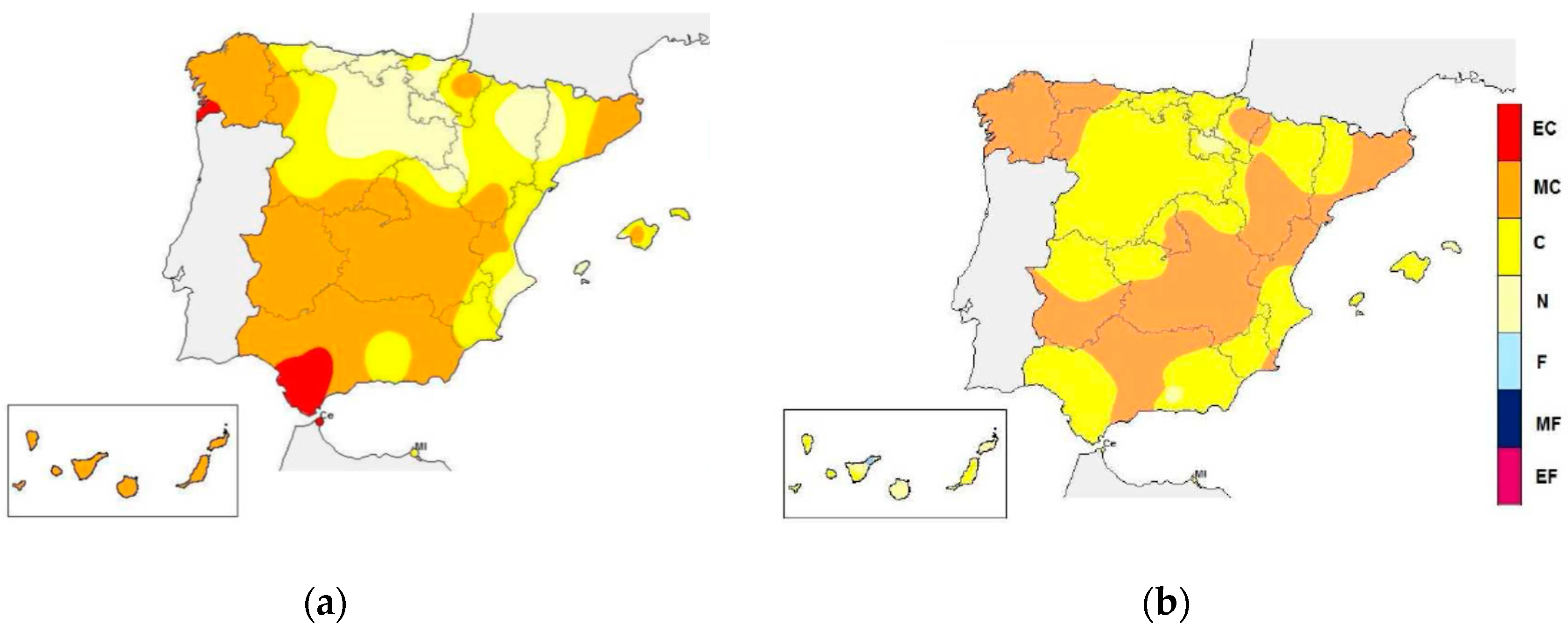
By performing a new analysis with the logarithmic data, the results are not improved. Hence, the problem must be related to the system (the summer is unexpectedly hot), the way the data are obtained from the system (the sensors), or the model (some assumptions are not correct). The analysis of the mean temperatures for the end of August and beginning of September proves, as the validation suggests, that summer of 2013 was hotter than expected in Seville [42,43], see Figure 14.

Since the source of the discrepancy between model and solution data is due to the use of climatic data that assume a usual summer, we discard from the temporal series those days that are over the normal temperature, mainly prior to 21 august. Higher maximum temperatures were generally registered in the first two days of the month, at the start of the second ten days and between 18 and 21, dates on which higher values of the month, above 40 °C, were reached in Extremadura and Guadalquivir. Major stations registered the following values on 19 days: Seville-airport 42.8 °C, Cordoba-Jerez de la Frontera with 41.7 °C and Morón de la Frontera airport 42.4 °C [43]. Moreover, the mean of the temperatures in our model was below 2.29 degrees (due to this unusually hot summer). Taking into account these adjustments to the model, we performed the test again, obtaining:

• Wilcoxon signed rank test
• data: Data.for.the.paper.by.day$Temperature_model_m[x] and Data.for.the.paper.by.day$Temperature_system[x]
• V = 190, p-value = 0.7265
• alternative hypothesis: true location shift is not equal to 0

The purpose of the model is not to predict the external temperatures, but it must be assured that the model predicts the ambient temperature of the building (or the room temperature because this is a key aspect of comfort). In the next section, the ambient temperature validation is analyzed.

4.2.3. Ambient Temperature

Continuing from the visual analysis of these data that we have previously done, we detect that the temperatures we obtain in the model are low in comparison with the system temperatures. As we previously detect, this is because the summer was too hot. Specifically, the mean of the system is about 34.92, while the mean for the model is 27.72 degrees Celsius. However, in the validation of the temperature, the offset between model and system temperature was only 2.29 degrees Celsius; this implies that something else is causing this gap (despite the unusualy hot summer). Reviewing the model assumptions, we detect that the ventilation of the building is quite high, causing a hyperventilation of the building. We modify our model according to these findings. The question that arises is if the obtained model data chart shapes (the curves, not the magnitudes) are correct despite this error.

Again, discarding the data prior to 21 August due to the unusual behavior of the temperature and considering the offset due to the hyperventilation for the chamber, we obtain:

• Wilcoxon signed rank test
• data: Data.for.the.paper.by.day$Ambient_model_m[x] and Data.for.the.paper.by.day$Ambient_system[x]
• V = 182, p-value = 0.8809
• alternative hypothesis: true location shift is not equal to 0

Clearly this shows that there is a relation between the model output and the system allowing us to validate the solution (the placement of the sensors, the new model hypotheses and the construction process performed).

4.3. Granger Causality

The daily means of the ambient temperature are analyzed, but the behavior of the whole shape of the time series must be also analyzed. The presence of Granger causality [44] does not assure a cause-effect relation. It may be that a third element exists that is not represented in the data that causes this. However, it is enough to determine that a relation exists between the two-time series. Hence, it can be concluded that the simulation output of the model can be used to analyze suitable alternatives in the system. “Granger causality tests are based on the notion of predictability, in particular whether past values of a variable X contain statistically meaningful information about current values of variable Y that is not contained implies the presence of a statistical causal ordering”. The application of Granger causality to environmental models was done first to analyze the anthropogenic influence on global temperature.

We can apply this test to understand if the system Ambient temperature can be predicted using the model Ambient temperatures. This helps in the determination of upcoming configurations of the façade parameters.

Applying this test to the complete dataset, we obtain:

• Granger causality test
• Model 1:
•   Data.for.the.paper.by.day$Ambient_system[x] ~Lags(Data.for.the.paper.by.day$Ambient_system[x], 1:1) + Lags(Data.for.the.paper.by.day$Ambient_model_m[x], 1:1)
• Model 2:
•   Data.for.the.paper.by.day$Ambient_system[x] ~Lags(Data.for.the.paper.by.day$Ambient_system[x], 1:1)
• Res.Df Df F Pr(>F)
• 1 22
• 2 23 −1 2.9019 0.1026

and

• Granger causality test
• Model 1:
•   Data.for.the.paper.by.day$Ambient_model_m[x] ~Lags(Data.for.the.paper.by.day$Ambient_model_m[x], 1:1)+Lags(Data.for.the.paper.by.day$Ambient_system[x], 1:1)
• Model 2:
•   Data.for.the.paper.by.day$Ambient_model_m[x] ~Lags(Data.for.the.paper.by.day$Ambient_model_m[x], 1:1)
• Res.Df Df F Pr(>F)
• 1 22
• 2 23 −1 0.204 0.6559

Meaning that the model data have a G-causal relation with the data we obtain for the system. From the point of view of the model validation, this assures there exists a relation between both time series. Going further, and considering that the model is based on time series and the model and the system must be related, a Robust Rank Correlation Coefficient and a Corresponding Test (implemented on the ROCOCO R package) can be performed [44]. This test indicates that between both time series there clearly exists a correlation, showing that the model is representing the behavior of the system at some level of correctness.

• Robust Gamma Rank Correlation:
• data: Data.for.the.paper.by.day$Ambient_system [x] and Data.for.the.paper.by.day$Ambient_model_m [x] (length = 26)
• similarity: linear
• rx = 0.2537676/ry = 0.2722265
• t-norm: min
• alternative hypothesis: true gamma is not equal to 0
• sample gamma = −0.03597242
• estimated p-value = 0.824 (824 of 1000 values)

This new analysis increases the confidence in the model, understanding that the Solution Validation achieves its main goals: test the model hypotheses, test the placement of the sensors, and test the construction process that has been followed to implement the proposed alternatives obtained from the simulation models.

5. Discussion

In the previous section, the Solution Validation for a small subset of the obtained data in the project has been shown. This validation helps us to detect problems in the hypotheses (the model) in the sensors (placement or monitoring errors) or in the boundary conditions (an unusually hot summer). Regarding this, it was quite interesting to detect that the external temperature has (as we suppose) a great impact on the models. This validation helps us to detect errors in the sensor placement and hypotheses. As shown in Section 4.1, some hypotheses lead us to obtain low temperatures for the ambient temperatures of the prototypes.

Visual inspection is a great tool to understand and detect discrepancies between the model and the system; see Figure 9. This visual inspection helps us to understand that the summer temperatures were unusually high, and we are able to corroborate this through a deeper analysis using historic climatic data.

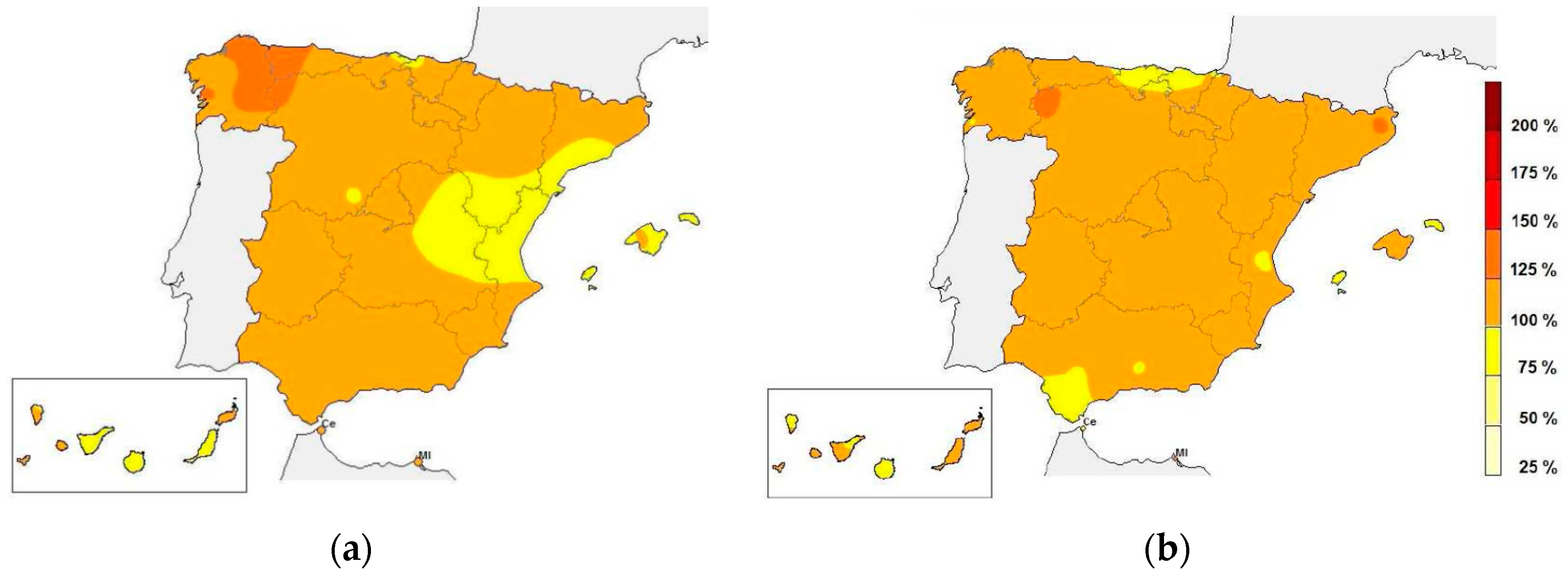
Analogously, it is quite interesting that the model behaves as expected when the boundary conditions are usual; this is the case of radiation, which was normal in Spain, and the solution validation corroborates this. See Figure 15 to see the radiation in Spain for the selected period.

Some interesting conclusions were obtained: the visual inspection of the data led us to understand that the general behavior of the models and the system are quite similar, a fact that led us to consider that the implementation accurately reflects the hypotheses for the model.

The model is sensitive (as it was supposed) to the boundary conditions (temperature, radiation, etc.). This implies that the ambient temperatures have the same patterns (as has been proved using the ROCOCO and Granger tests) but with a displacement in the vertical axis (due to the unusual boundary conditions discussed here). It is quite interesting that the detection of the hyperventilation in the chamber is due to an incorrect configuration.

According to the analyzed data (summer time), the operation at the level of energy demand for both façades (photovoltaic façade and double façade with lamas) is similar. It is worth mentioning that the façade with slats (the analyzed here), which allows us to control direct solar light, and its results could have been better if the air volume ventilation between outside and the air chamber would have been higher (allowing a better renewal of air and, thus, avoiding pockets of heat accumulated during the day in the chamber). According to the validation, the slats would serve to collect and capture solar heat, accumulate it and expel it to the interior of the room, helping to heat the room; the thermal time delay is already established, in part, with these results.

According to this validation, the model of the new façades accurately represents the ambient temperature of the building; we can use it to parameterize and propose alternatives prior to constructing a new building to achieve the comfort needed, see Table 1.

6. Concluding Remarks

In this paper, a Solution Validation case study has been shown. This case of validation is rare mainly because it must be done once a decision has been made regarding system belief in the simulation results and its recommendations are applied (implemented) in the system. This paper represents a case study that can be shown as an example of a complete Solution Validation. In this case study, we propose using some specific statistical techniques in order to establish a correspondence between the time series that are provided by the model and by the monitored system. This allows us to understand if the model accurately represents the system expected behavior, taking into account the considered hypotheses.

The recalibration of the models due to the solution validation was successful, allowing the subsequent use of models in different climatic zones. In addition, the model can be adjusted further, since the slots of the air conditioning system, ventilation air volume, the mass of lamas and climate data are not completely coincidental. However, it has been corroborated that the final implementation of the system, following the directions proposed for the model results, is effective, efficient and produces important savings of time and money.

Solution Validation helps in the needed continuous Accreditation of the simulation model, becoming a key element to understand possible mistakes in the hypotheses of the model with respect to its codification or in the process followed to implement the solution. Those aspects are key elements if the simulation model is going to be used several times to define new and good solutions for other equivalent, or similar, systems. The main drawbacks of solution Validation are related to the time needed to perform such analysis once the project has been Accredited, meaning that the contractor believes in the accuracy of the model. However, if the model must be used as an element to make decisions in new scenarios, this kind of Validation must be considered as a substantial part of the whole simulation study.