Segmentation of Residential Gas Consumers Using Clustering Analysis

Abstract

The growing environmental concerns and liberalization of energy markets have resulted in an increased competition between utilities and a strong focus on efficiency. To develop new energy efficiency measures and optimize operations, utilities seek new market-related insights and customer engagement strategies. This paper proposes a clustering-based methodology to define the segmentation of residential gas consumers. The segments of gas consumers are obtained through a detailed clustering analysis using smart metering data. Insights are derived from the segmentation, where the segments result from the clustering process and are characterized based on the consumption profiles, as well as according to information regarding consumers’ socio-economic and household key features. The study is based on a sample of approximately one thousand households over one year. The representative load profiles of consumers are essentially characterized by two evident consumption peaks, one in the morning and the other in the evening, and an off-peak consumption. Significant insights can be derived from this methodology regarding typical consumption curves of the different segments of consumers in the population. This knowledge can assist energy utilities and policy makers in the development of consumer engagement strategies, demand forecasting tools and in the design of more sophisticated tariff systems.

1. Introduction

The energy sector constitutes the source of at least two-thirds of greenhouse gas emissions, which means action must be undertaken to reduce energy consumption and the associated greenhouse gas emissions. According to the World Energy Outlook 2016 Report [1], there will be a 30% rise in global energy demand to 2040. Globally, it is predicted that renewable energy will see by far the fastest growth [1]. Natural gas, as the cleanest fossil fuel, can be considered as an important adjunct to renewable energy sources [2]. Therefore, it is expected that gas consumption will increase worldwide, where the potential for demand growth will be significant in Asia, while Japan will fall back as nuclear power is reintroduced [1,3].

The European Commission adopted measures aimed at achieving savings of 20% in primary energy consumption until 2020 [4]. Some of these measures strongly focus on the residential sector, an important target of energy policy where potential energy savings can be achieved [4,5,6]. Residential consumers give preference to natural gas energy for heating, cooking and hot water over other sources of energy, for being environmentally-friendly, easy to use and reliable, in terms of distribution and supply and eventually less expensive compared to other sources. Smart grids play a relevant role in this matter by empowering consumers to make smarter decisions regarding the use of energy in their household.

The emerging smart grid requires distributed intelligence, as well as the development of models based on artificial intelligence, e.g., [7,8,9]. Several studies have been published in the electrical energy field, mostly facilitated by the availability of suitable databases [10]. Different is the case for research on the analysis of gas demand, especially when it comes to clustering and consumer profiling based on consumption data. These data can provide significant insights for utilities and policy makers regarding typical consumption curves of the different segments of consumers. The effect of energy policy on the different segments of consumers can be studied based on the way these different segments consume this energy source. A substantial amount of effort has been put into the gas demand forecasting [11,12,13,14,15,16] and into the determinant factors of residential gas consumption [17,18]. The study of energy savings has been conducted for buildings, as well, mostly inserted in projects for the development of sustainable cities [19,20]. The investigation of the weather impact on energy consumption is also addressed in the literature. The gas sector is one of the most sensitive sectors affected by weather risk and time of year [21,22,23,24,25], since there is higher gas demand in colder seasons compared to warmer seasons.

Regarding the use of clustering techniques for residential gas consumers’ load profiling, few papers have been published. In a study [26] from 2009, gas standardized load profiles (SLP) were obtained by using clustering as part of the development of a semiparametric regression model. Consumers were classified according to their classes (household and small and medium commercial), type (household, office, manufacturer, heating plant, etc.) and gas appliances (heating, cooking, hot water and technology). Then, the authors used Ward’s hierarchical clustering (HC) [27] and the K-means (KM) clustering algorithm [28] to obtain the clusters of consumers in the population. For the model implementation, the consumers were classified into the resulting segments obtained, where the most suited type of estimated SLP curves was assigned to them. In [29,30], a clustering analysis was performed to determine the segmentation of residential gas consumers. In [29], fuzzy C-means (FCM) [31], KM algorithms and HC were used to obtain seasonal representative profiles of gas consumers. These were characterized based on the consumption patterns; however, the consumers’ socio-economic and household key features were not considered. In [30], the segments were characterized based on the consumption patterns and on the consumers’ socio-economic and household key features; however, a single clustering technique was used.

In this paper, we propose a methodology to determine the segmentation of residential natural gas consumers using clustering techniques. This analysis is novel for the case of natural gas profiling for two reasons. The first is because we use more than a clustering algorithm to obtain the segments. The second relies on the fact that we characterize these segments based not only on the representative profiles obtained from clustering, as well as according to information regarding consumers’ socio-economic and household key features. We use three clustering algorithms, namely KM, FCM and Ward’s HC, to define the profiles of consumers. Classical KM is one of the most used clustering algorithms to obtain energy consumption profiles. Both KM and FCM have already been successfully used for the case of smart metering electricity data [32,33,34,35,36,37,38,39,40,41] and natural gas data [26,30]. FCM allows gradual memberships to cluster, which offers the opportunity to deal with data that belong to more than one cluster simultaneously [31]. Besides partitioning methods, Ward’s method was selected for being an agglomerative hierarchical clustering technique and because it has already been applied to natural gas data [26,29]. A logistic regression is performed to link the socio-economic and household key features to the groups of consumers obtained with clustering.

We use clustering validity indices (CVIs), namely silhouette, Davies and Bouldin’s index, Dunn’s validity index, weighted average intra-inter cluster distance index and Xie and Beni’s index, to evaluate the results obtained from the clustering algorithms referred to above. These CVIs were selected because they all focus on maximizing intra-cluster and minimizing inter-cluster similarities. Davies and Bouldin’s and Dunn’s validity indices are well-known measures, frequently used for the task of selecting the best clustering solution [42]. The weighted average intra-inter cluster distance index was selected because it gives a measure of the overall cluster quality [43]. Silhouette combines both cohesion and separation, and the average silhouette width provides an evaluation of clustering validity, which can be visually assessed in a graphical representation [44]. Finally, Xie and Beni’s index proved to be suited for assessing clustering results, particularly for the FCM algorithm [45].

We analyze the seasonal clusters obtained and draw conclusions regarding the consumption curves and characteristics of each cluster. High frequency smart metering gas consumption data from Ireland [46] are used. The database is rich since it contains data of approximately one and a half thousand households over one and a half years.

The outline of the paper is as follows. In Section 2, we present the data preprocessing steps. In Section 3, we address the clustering techniques and the CVIs. In Section 4, we evaluate and discuss the clustering results and the specific characteristics of each segment of gas consumers. In Section 5, we present the conclusions of this research and future work.

2. Data Preprocessing

Smart metering data consist of consumption data recorded in a smart meter device in intervals of an h or less. In order to obtain the profiles of consumers for an easier interpretation and analysis, preprocessing was performed. The data preprocessing adopted in the paper is represented in Figure 1.

Data collected from smart meters may exhibit missing values, e.g., due to noise. The missing data may be replaced by appropriate values or left as missing. In the paper, missing data were ignored, given that the aggregation task reduced this impact on the overall data quality. The missing data analysis was followed by a process of context filtering, which involved the selection of data representing a specific context such as a temporal window, type of day and location. Regarding the outliers’ analysis, all households with a significant percentage of null consumption measurements were considered outliers and excluded. In the task of data aggregation, the period used (e.g., monthly, weekly) and operator (e.g., sum, median) have to be defined. The operator of summation was used to aggregate consumption data hourly per season for each consumer, as presented in Figure 2. “Day A” corresponded to the aggregated hours of a day for a consumer in the respective season. Thus, for H input features and N consumers, the feature vector for consumer k is $\mathbf{x}=[x_{k_1},\dots ,x_{k_H}]$ where k = 1:N, $X\in {\mathrm{I}\mathrm{R}}^{N\times H}$ contained the information in matrix of (1).

$$\begin{array}{c}\hfill X=\left[\begin{array}{ccc}{x}_{1_1}& \cdots & x_{1_H}\\ ⋮& \ddots & ⋮\\ x_{N_1}& \cdots & x_{N_H}\end{array}\right]\end{array}$$

(1)

In this paper, the profiles were normalized based on the maximum hourly consumption of all consumers, using the minimum-maximum normalization method:

$$x_{norm}=\frac{x-x_{min}}{x_{max}-x_{min}}$$

(2)

where $x_{norm}$ is the normalized version of the feature value x to be normalized. $x_{max}$ and $x_{min}$ are the maximum and minimum value of feature x, respectively. This method is commonly used in engineering and clustering applications to normalize the data due to its linear transforming form [47].

3. Clustering

Data clustering is a method of creating groups of objects, or clusters, in such a way that objects in one cluster are similar and objects in different clusters are distinct [48]. In this paper, we used clustering methods in a specified context, such as a season, to obtain the segments of consumers. Figure 3 presents the methodology we followed to determine the segments of consumers and their respective representative profiles. The clustering analysis was similar to the one proposed in [49] for the case of electricity smart metering data. This analysis consists of processing smart metering data to obtain the representative profiles of consumers. Clustering configurations are tested and assessed by means of CVIs. Expert judgement is also used in this step, through graphical visualization of the clusters obtained. Once a clustering configuration is selected, the representative profiles of the population are obtained.

3.1. Clustering Algorithms

A clustering algorithm is mainly characterized by a proximity measure, which quantifies how “similar” two data points are, and a clustering criterion, as well as by its efficiency to define a clustering scheme that fits the dataset [50]. The clustering criterion is expressed via a cost function in the case of the partitioning algorithms or via the termination condition where data objects are grouped into a tree until a single cluster remains, in the case of hierarchical clustering. The objective functions serve as cost functions that have to be minimized to obtain optimal cluster solutions.

3.1.1. K-Means

Hard c-means, better known as K-means (KM), is classified as a partitional clustering algorithm, where the number of clusters ($n_c$) is assumed to be fixed [28]. In the KM algorithm, the clusters are represented by the center vectors $\overline{{\mathbf{c}}_i}$. It is required that the set of clusters $\mathbf{C}=\{c_1,\dots ,c_{n_c}\}$ is a partition of the dataset into non-empty pairwise disjoint subsets. Such a data partition is said to be optimal when the sum of the squared distances between the cluster centers and the data points assigned to them is minimal. The objective function of the KM algorithm is the following:

$${\displaystyle {\mathbf{J}}_h(\mathbf{X},{\mathbf{U}}_h,\mathbf{V})=\sum _{i=1}^{n_c}\sum _{j=1}^N{\mathit{\mu }}_{ij}{d}_{ij}^2({\mathbf{x}}_j,\overline{{\mathbf{c}}_i})}$$

(3)

where ${\mathbf{U}}_h$ is the partition matrix $n_c\times N$ and $\mathbf{V}=\{\overline{{\mathbf{c}}_1},\dots ,\overline{{\mathbf{c}}_{n_c}}\}$ is the set of cluster centers. The Euclidean distance is represented by $d_{ij}$, and ${\mathit{\mu }}_{ij}\in \{0,1\}$ indicates the assignment of data to clusters. Each data point is assigned to its closest cluster center according to the formula:

$${\mu }_{ij}=\left\{\begin{array}{cc}1,\hfill & \mathrm{if}i={\mathrm{argmin}}_{l=1}^{n_c}{d}_{lj}\hfill \\ 0,\hfill & \mathrm{otherwise}\hfill \end{array}\right.$$

(4)

The calculation of the mean for each cluster is in (5):

$${\overline{\mathbf{c}}}_i=\frac{{\sum }_{j=1}^N{\mathit{\mu }}_{ij}{\mathbf{x}}_j}{{\sum }_{j=1}^N{\mathit{\mu }}_{ij}}$$

(5)

3.1.2. Fuzzy C-Means

FCM was developed by J.C.Dunn in 1973 [31] and improved by J.C. Bezdek in 1981 [51]. Fuzzy cluster analysis allows gradual memberships of data points to clusters ${\mathit{\mu }}_{ij}\in$ [0, 1] in ${\mathbf{U}}_f$. The objective function of the FCM algorithm is the following:

$${\displaystyle {\mathbf{J}}_f(\mathbf{X},{\mathbf{U}}_f,\mathbf{V})=\sum _{i=1}^{n_c}\sum _{j=1}^N{\mathit{\mu }}_{ij}^m{d}_{ij}^2({\mathbf{x}}_j,\overline{{\mathbf{c}}_i})}$$

(6)

The parameter m, where $m>$ 1, is the weighting exponent, which determines the ‘fuzziness’ of the classification. For the FCM algorithm, the membership degrees are selected according to (7):

$${\mu }_{ij}=\frac{1}{{\displaystyle \sum _{l=1}^{n_c}{\left(\frac{d_{ij}^2}{d_{lj}^2}\right)}^{\frac{1}{m-1}}}}=\frac{d_{ij}^{-\frac{2}{m-1}}}{{\displaystyle \sum _{l=1}^{n_c}{d}_{lj}^{-\frac{2}{m-1}}}}$$

(7)

The fuzzy partition matrix ${\mathbf{U}}_f$ is held fixed, and the calculation of the mean for each cluster is:

$${\overline{\mathbf{c}}}_i=\frac{{\sum }_{j=1}^N{\mathit{\mu }}_{ij}^m{\mathbf{x}}_j}{{\sum }_{j=1}^N{\mathit{\mu }}_{ij}^m}$$

(8)

3.1.3. Hierarchical Clustering

Ward’s minimum variance method is a hierarchical agglomerative clustering algorithm [27]. Ward’s method finds in each iteration the pair of clusters that leads to the minimum increase in total within-cluster variance after merging. We used the weighted squared Euclidean distance as linkage measure. Ward’s method first selects the most appropriate $n_c$ and considers each sample as a cluster in order to calculate the square sum of each cluster deviation. Each cluster is combined until all samples with higher similarity are in the same cluster.

3.2. Clustering Validity Indices

The number of clusters $n_c$ in the data is usually unknown, so it has to be specified as an input parameter. The CVIs used to assess the optimal $n_c$ in the data are introduced as follows. The aim is to maximize the intra-cluster and minimize the inter-cluster similarities.

3.2.1. Silhouette Index

The silhouette (Sil) [44] consists of a method of interpretation and validation of consistency within clusters:

$${\displaystyle Sil=\frac{1}{N}\sum _{c_k\in \mathbf{C}}\sum _{{\mathbf{x}}_i\in c_k}\frac{b({\mathbf{x}}_i,c_k)-a({\mathbf{x}}_i,c_k)}{max\{a({\mathbf{x}}_i,c_k),b({\mathbf{x}}_i,c_k)\}}}$$

(9)

where:

$${\displaystyle a({\mathbf{x}}_i,c_k)=1/|c_k|\sum _{{\mathbf{x}}_j\in c_k}d({\mathbf{x}}_i,{\mathbf{x}}_j)}$$

(10)

and:

$${\displaystyle b({\mathbf{x}}_i,c_k)=\underset{c_l\in \mathbf{C}\backslash c_k}{\min }\left\{1/|c_l|\sum _{{\mathbf{x}}_j\in c_l}d({\mathbf{x}}_i,{\mathbf{x}}_j)\right\}.}$$

(11)

Values $a({\mathbf{x}}_i,c_k)$ and $b({\mathbf{x}}_i,c_k)$ are a measure of cohesion and isolation, respectively. Entities with a Sil width close to one are well clustered, while those with a lower width can be considered intermediate.

3.2.2. Davies–Bouldin Index

The Davies and Bouldin’s index (DB) [52] identifies compact clusters that are far from each other, and it is defined as:

$${\displaystyle DB=\frac{1}{n_c}\sum _{c_i\in \mathbf{C}}\underset{c_k\in \mathbf{C}\backslash c_i}{\max }\left\{\frac{s(c_i)+s(c_k)}{d(\overline{{\mathbf{c}}_i},\overline{{\mathbf{c}}_k})}\right\}}$$

(12)

where:

$${\displaystyle s(c_k)=1/|c_k|\sum _{{\mathbf{x}}_j\in c_k}d({\mathbf{x}}_j,\overline{{\mathbf{c}}_k}).}$$

(13)

It is desirable for the clusters to have the minimum possible similarity to each other; therefore, the best clustering results are given by a minimum value of the index.

3.2.3. Dunn’s Index

The Dunn’s validity index (DI) is used to identify “compact and well separated” [53] clusters. The index for a specific number of clusters is defined as:

$$DI=\underset{1\le i\le n_c}{\min }\{\underset{1\le j\le n_c,j\ne i}{\min }\left\{\frac{{\delta }_D(c_i,c_j)}{\underset{1\le k\le n_c}{\max }{\Delta }_D(c_k)}\right\}$$

(14)

where:

$${\delta }_D(c_i,c_j)=\underset{\mathbf{x}\in \overline{c_i},\mathbf{y}\in \overline{c_j}}{\min }d(\mathbf{x},\mathbf{y})$$

(15)

and:

$${\Delta }_D(c_k)=\underset{\mathbf{x},\mathbf{y}\in c_k}{\max }d(\mathbf{x},\mathbf{y})$$

(16)

Equations (15) and (16) represent the inter- and intra-cluster distances, respectively. The best clustering results are obtained with the maximum value of the index.

3.2.4. Weighted Intra-Inter Index

The weighted average intra-inter cluster distance index (WI) was proposed by Strehl [43], and it is based on the ratio of the weighted average inter-cluster to the weighted average intra-cluster similarity:

$$WI=(1-2n_c{/}_N)\left(1-\frac{{\sum }_{i=1}^{n_c}\frac{|c_i|}{N-|c_i|}{\sum }_{j\in \{1,\dots ,i-1,i+1,\dots ,n_c\}}|c_j|·{\delta }_W(c_i,c_j)}{{\sum }_{i=1}^{n_c}|c_i|{\Delta }_W(c_i)}\right)$$

(17)

where:

$${\displaystyle {\delta }_W(c_i,c_j)=\frac{1}{|c_i|·|c_j|}\sum _{\mathbf{x}\in \overline{c_i},\mathbf{y}\in \overline{c_j}}d(\mathbf{x},\mathbf{y})}$$

(18)

and:

$${\displaystyle {\Delta }_W(c_i)=\frac{2}{(|c_i|-1)|c_i|}\sum _{\mathbf{x},\mathbf{y}\in c_i}d(\mathbf{x},\mathbf{y})}$$

(19)

Inter- and intra-cluster distances are represented by (18) and (19), respectively. A null WI indicates that objects within the same cluster are on average not more similar than objects from different clusters. On the contrary, for a WI of one, all pairs of objects from different clusters have a similarity of zero, and at least one pair from the same cluster has a non-zero similarity.

3.2.5. Xie and Beni’s Index

Xie and Beni [54] defined an index of fuzzy cluster validity (with the parameter m = 2), which was later generalized by Pal and Bezdek [45]. Cluster compactness and separateness are measured by using:

$$XB=\frac{{\displaystyle \sum _{i=1}^{n_c}\sum _{j=1}^N{({\mathit{\mu }}_{ij})}^m{\mathrm{d}}_{ij}^2({\mathbf{x}}_j,{\mathbf{v}}_i)}}{N\underset{i,j}{\min }{\mathrm{d}}_{ij}^2(\overline{{\mathbf{c}}_i},\overline{{\mathbf{c}}_j})}$$

(20)

The optimal $n_c$ should be obtained with the minimum value of the index.

4. Results and Discussion

4.1. Natural Gas Data Preprocessing

The gas consumption data, as well as the socio-economic features of consumers and household characteristics were provided by the Irish Social Science Data Archive (ISSDA) [55]. The smart metering gas consumption data (in kWh) were collected from 1 December 2009–30 May 2011 with a frequency of a half an h in each day. Smart metering data from 1493 households were available for preprocessing.

4.1.1. Missing Data Analysis

Six days were missing in the database. We ignored these days, since there was no obvious way to attribute the gas use. We considered that the available data had a significant extent and their absence would not affect the following steps of data preprocessing. Moreover, the aggregation task would reduce this impact on the overall data quality.

4.1.2. Context Filtering

We excluded weekends and holidays from the analysis since they represented atypical periods of consumption. Thus, we used only smart metering data from working days. Then, we extracted the profiles seasonally, by aggregating days for each season of a year. We used data from December of 2009–2010. The way we divided data for each season is presented in

Table 1. Data division for each season, in accordance with the Irish calendar.

Season	Dates	Year	Days
Winter	21 December–19 March	2009/2010	57
Spring	20 March–20 June	2010	61
Summer	21 June–22 September	2010	65
Autumn	23 September–20 December	2010	60

. The corresponding number of days to be aggregated was 243.

4.1.3. Outliers Analysis

We observed that there were households with low gas use throughout the study period. These may correspond to holidays or renting accommodation households, which were considered exceptions. Therefore, after data analysis, we considered that all consumers with more than 90% of null consumption measurements in the study period should be excluded. With the removal of these outliers, we obtained more defined and compact representative profiles of consumers. With this criterion, we excluded 63 consumers and were left with 1430. An example of a standard and of a low gas use profile in a year is depicted in Figure 4.

4.1.4. Data Aggregation

We performed an hourly aggregation of all consumption data, obtaining 24 features for each consumer in each season, as presented in Figure 2 of Section 2. We used summation as the aggregation operator in order to keep the value of total amount of gas consumption for each consumer. Given N samples (here, N = 1430) and H input features (here, H = 24), we constructed a matrix for each season, as given in (1).

4.1.5. Data Normalization

We normalized the profiles of consumers using the minimum-maximum normalization method (2), based on the maximum hourly consumption of all consumers for each season. By using a normalization, the normalized consumption curves provided more insights related to the patterns of consumption, and the profiles were more defined.

4.2. Seasonal Consumptions

The profile curves of the seasonal mean hourly aggregated consumption of all consumers are depicted in Figure 5.

As expected, winter, the coldest season, presents the highest mean hourly aggregated consumptions, while summer, the warmer season, presents the lowest. This happens because gas is mainly used for bathing and cooking in the summer, while in the winter, it is also needed for heating. For every season, there are two evident consumption peaks, one in the morning and the other in the evening. Mean hourly aggregated consumptions are low during the night and, in the case of summer, practically null.

4.3. Seasonal Profiles

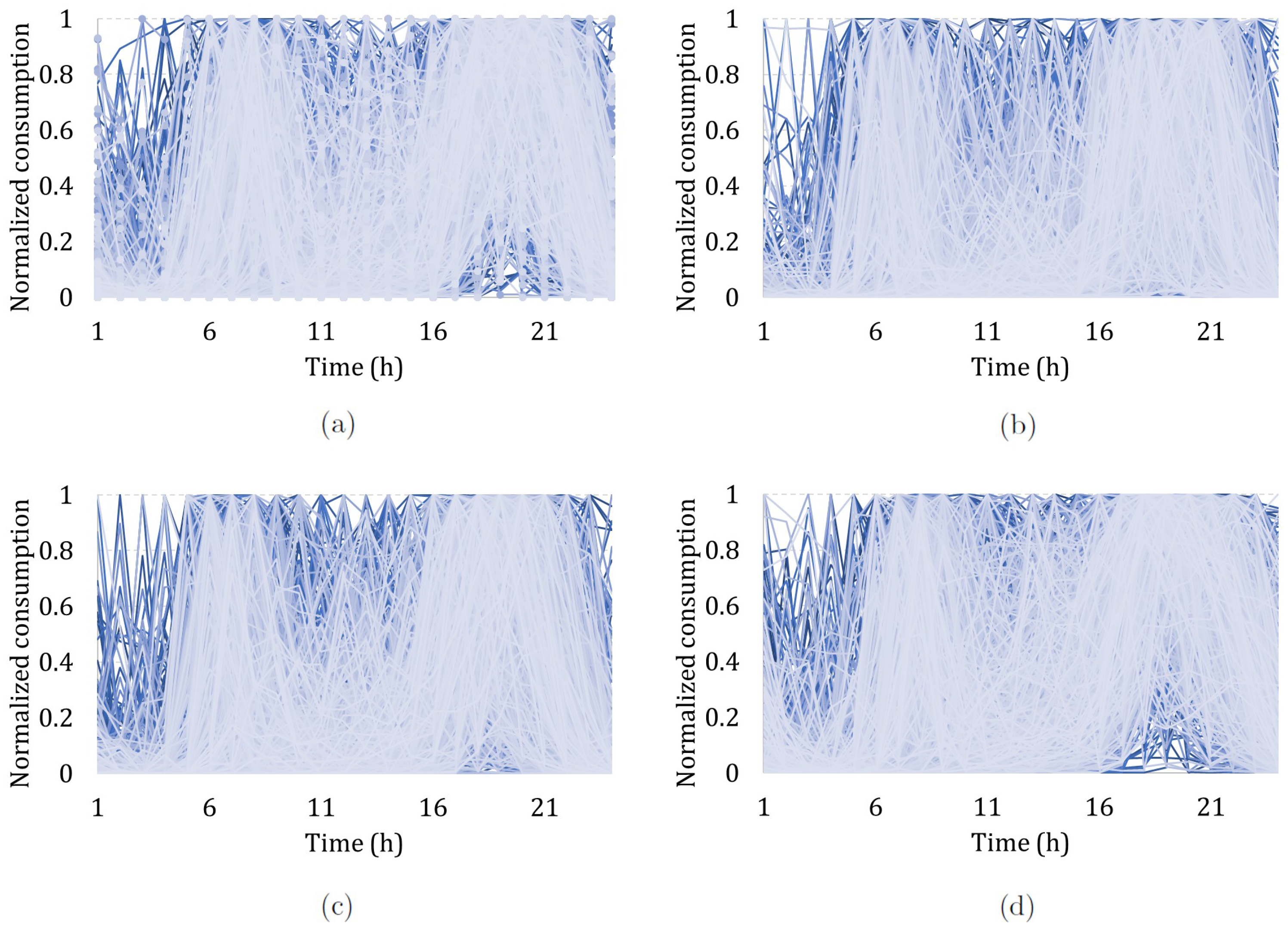
Before performing clustering analysis, we assessed the normalized consumption patterns of consumers for each season and concluded that there was no structure, as it can be seen in Figure 6. In order to obtain the seasonal profiles, we performed clustering with classical KM and FCM algorithms and Ward’s HC, using MATLAB software. We used the five CVIs presented in Section 3.2 to assess clustering results. In order to obtain the best clustering configurations, we varied $n_c$ between two and 10. We considered that the best clustering configuration should present a uniform distribution, minimize intra-cluster distance and maximize inter-cluster distance.

Since the KM algorithm depends on the initialization, we performed ten iterations for each number of clusters ($n_c$) and selected one that presented the best CVI values. For the FCM algorithm, we varied m between 1.25 and two. The best results were achieved with an m of 1.25; therefore, we only present the results obtained with this parameter value.

Clustering results presented in

Table 2. Selected $n_c$ (with respective clustering validity index (CVI) score), for each algorithm and season. DB, Davies and Bouldin’s index; DI, Dunn’s validity index; WI, weighted average intra-inter cluster distance index; Sil, silhouette.

Seasons	Algorithms	XB (↓)	DB (↓)	DI (↑)	WI (↑)	Sil (↑)
Spring	KM	2 (0.82)	5 (1.73)	2 (0.84)	4 (0.59)	2 (0.31)
	HC	3 (1.25)	6 (1.99)	2 (0.72)	3 (0.74)	2 (0.23)
	FCM	2 (1.60)	4 (1.82)	2 (0.82)	5 (0.58)	2 (0.30)
Summer	KM	2 (0.77)	5 (1.40)	2 (0.75)	5 (0.76)	2 (0.46)
	HC	4 (1.69)	4 (1.45)	2 (0.62)	8 (0.68)	4 (0.30)
	FCM	2 (0.91)	5 (1.69)	2 (0.73)	3 (0.75)	2 (0.45)
Autumn	KM	2 (0.83)	2 (1.80)	2 (0.94)	3 (0.62)	2 (0.24)
	HC	4 (1.24)	4 (1.84)	2 (0.78)	4 (0.71)	2 (0.17)
	FCM	2 (0.88)	5 (1.60)	2 (0.93)	5 (0.60)	2 (0.24)
Winter	KM	5 (1.10)	5 (1.80)	2 (0.88)	5 (0.66)	2 (0.23)
	HC	5 (1.60)	5 (2.08)	2 (0.77)	7 (0.65)	5 (0.08)
	FCM	2 (1.01)	5 (1.62)	2 (0.88)	5 (0.67)	2 (0.23)

are based on the CVI scores, as well as expert judgment. The criterion to select the algorithm and number of clusters consisted of selecting the algorithm where there was a higher number of CVI agreement on the number of clusters. We provide the results of the CVI scores for each $n_c$ in Appendix A.

DI consistently indicated two as the best $n_c$, as well as Sil, except for two events with HC, as presented in Table 2. When analyzing the representative profiles obtained with two clusters, we observed that, for all seasons, it consisted of a separation between high and low consumption consumers, as presented in Appendix B. In this scenario, the majority of the profiles were significantly different from the representative ones. For this reason, we considered that a more interesting analysis regarding the consumption profiles should be performed with a higher $n_c$. Thus, the best $n_c$ obtained for spring and summer was three, with the HC and FCM algorithm, respectively, for autumn was four with HC and for winter was five with the KM algorithm. The selection of algorithms and $n_c$ for each season was based on the following rationale:

• Spring, HC with three clusters: HC was the algorithm where two CVIs agreed regarding the best number of clusters to select;
• Summer, FCM with three clusters: Although two CVIs agreed on five clusters for KM and three CVIs agreed on four clusters for HC, for both, one of the clusters was not representative of the population, with a reduced number of consumers. For FCM, two CVIs presented the highest values for five (DB) and three (WI) clusters. Following the elbow method, where an inferior $n_c$ is chosen since adding more clusters does not improve clustering results, three clusters were selected. These clusters were compact, well defined and representative of the population;
• Autumn, HC with four clusters: HC was the algorithm where three CVIs agreed regarding the best number of clusters to select;
• Winter, KM with five clusters: Both the KM algorithm and HC had three CVIs that agreed on the number of clusters; however KM, presented more compact clusters, which was assessed by visual analysis.

In the following figures illustrating the normalized consumption profiles of the consumers, the x-axis represents the 24 h in a day.

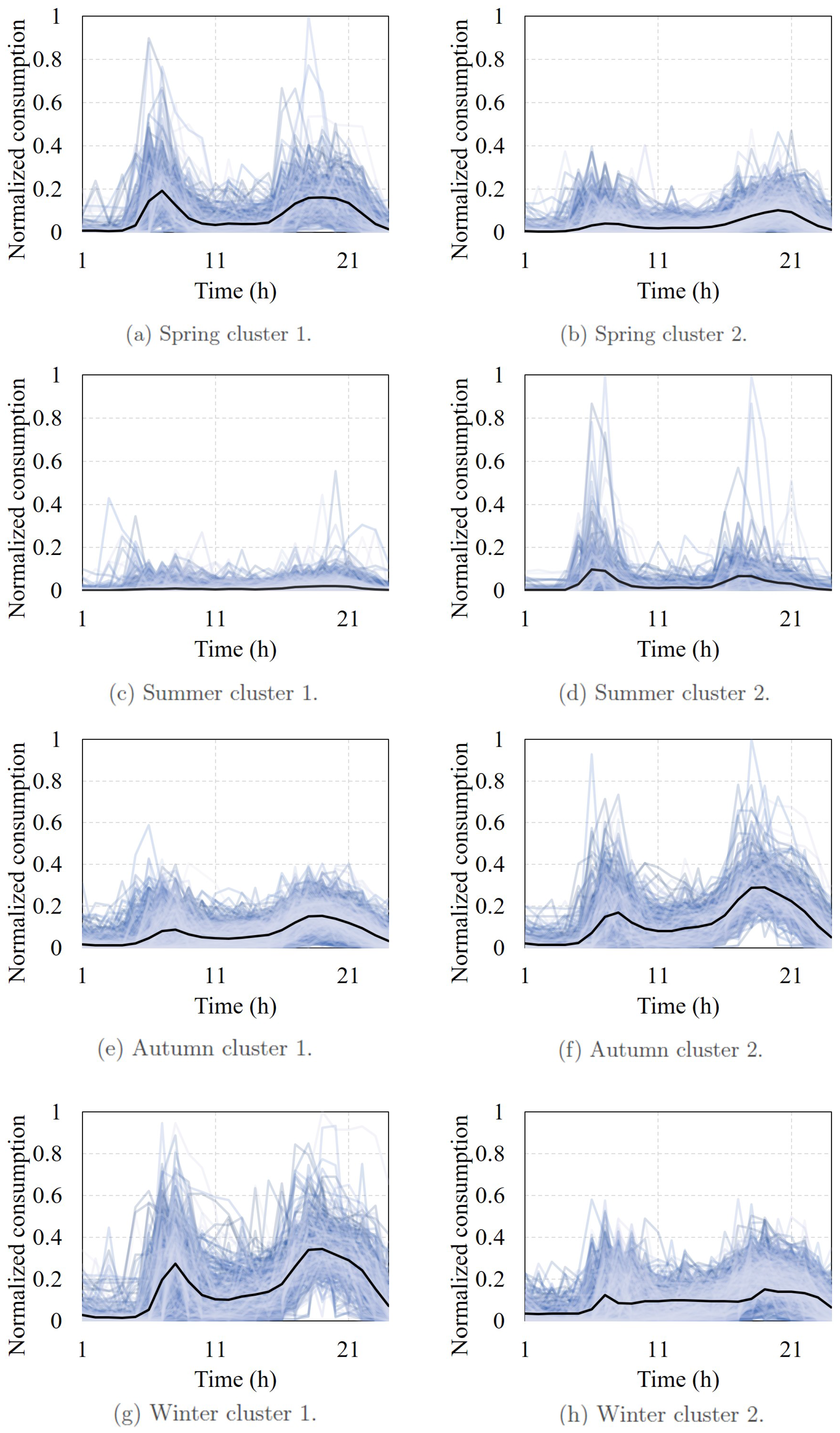
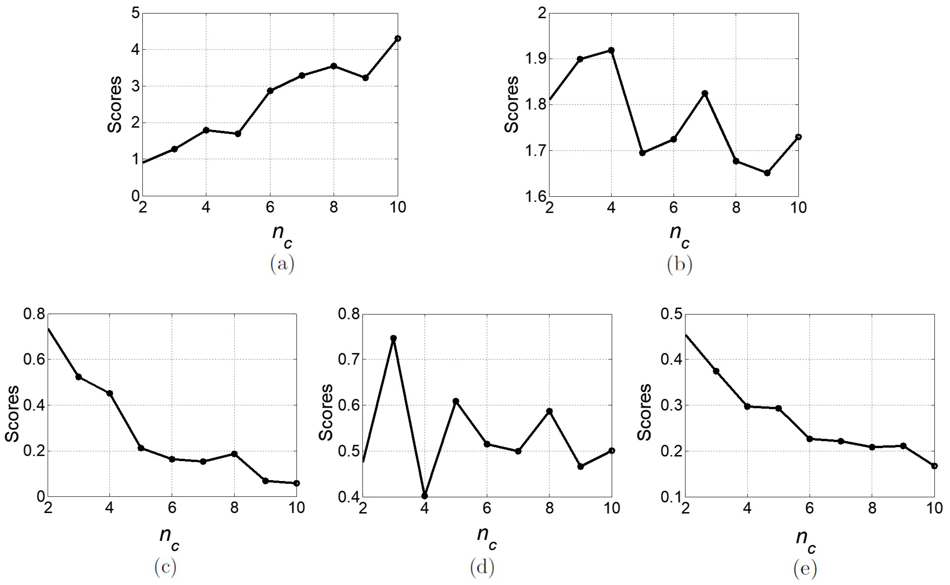
The spring profiles are presented in Figure 7, where three clusters were obtained using HC. From Figure 8, it can be observed that WI and XBpresented higher performance with this $n_c$. DI and Sil also presented a high value for three clusters, very similar to the ones obtained with two clusters.

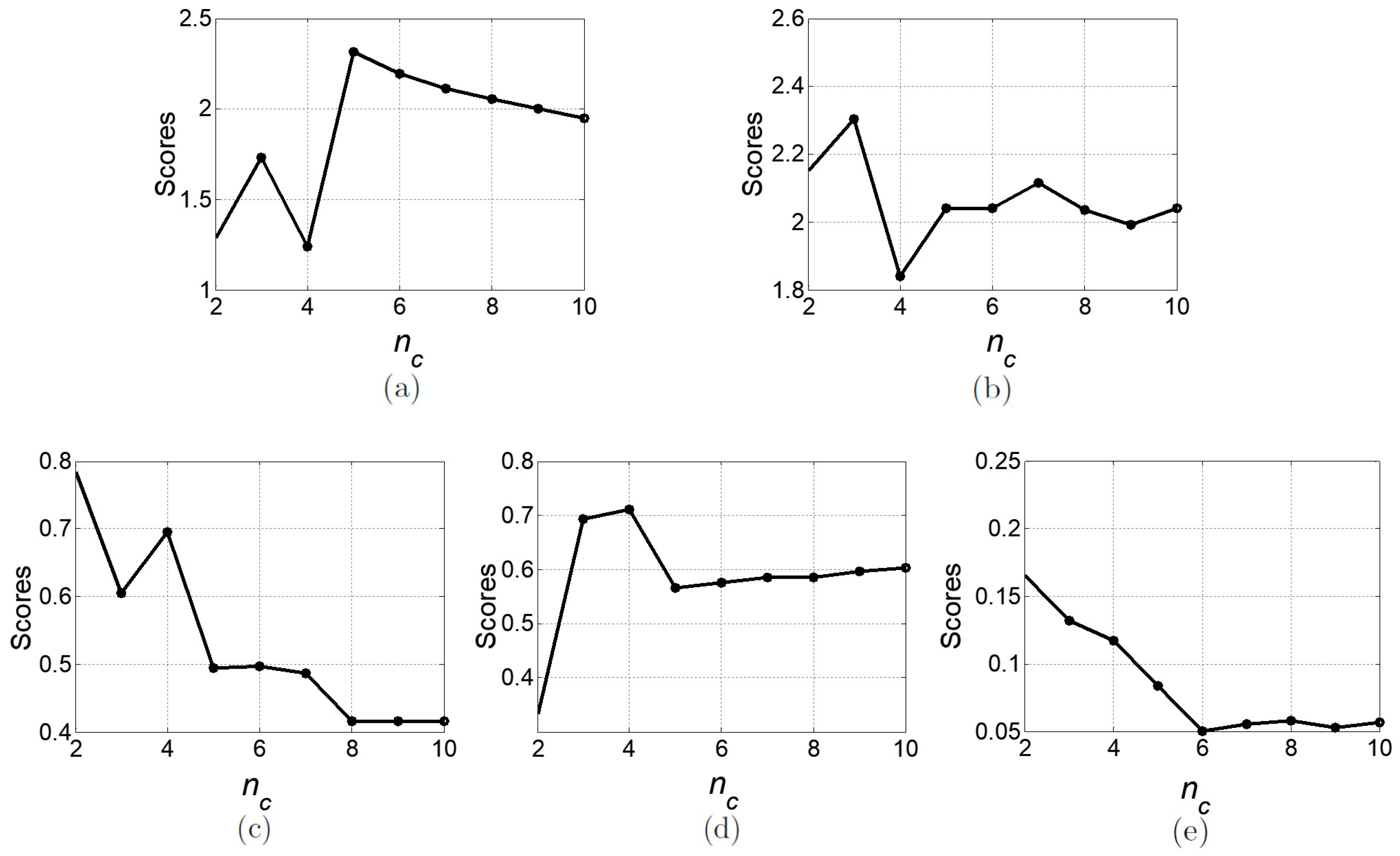
The summer profiles are presented in Figure 9, where three clusters were obtained using the FCM algorithm. This $n_c$ was mainly indicated by WI, as noticeable in Figure 10. We considered the higher degree of membership of a consumer to a cluster to turn fuzzy memberships into crisp partitions. With three clusters, higher CVI performance results were achieved with the HC and KM algorithm. However, for both, one of the clusters had a reduced number of consumers. These clusters were not considered representative of the population; therefore, results obtained with FCM algorithm were selected.

The XB index is suited to assess the clustering results of the FCM algorithm; however, this CVI consistently indicated two clusters as the best $n_c$, as can be seen in Table 2. For the case of summer, analyzing the XB index in Figure 10, there is an elbow point for five clusters. The elbow point consists of the number of clusters with a sharp change of the index values, and it is a method of selecting the best number of clusters. However, between three and five clusters, three were selected, following the principle of the elbow method, where an inferior $n_c$ is chosen since adding more clusters does not improve clustering results. The three clusters obtained were compact, well defined and representative of the population.

The autumn profiles are presented in Figure 11, where four clusters were obtained using HC. The clusters obtained with HC were more compact and well defined, compared to the other algorithms, and presented consistent CVIs performance, which can be verified in Figure 12.

The winter profiles are presented in Figure 13, where five clusters were obtained using the KM algorithm. For this algorithm, all CVIs indicated five clusters as the best result, except for Sil and DI. Although Sil and DI presented the best result for two clusters, five clusters were the second best result for both, which can be observed in Figure 14. The clusters obtained with KM were more compact and well defined, compared to HC. For the HC and FCM algorithm, five clusters were selected as the best by at least two CVIs, which can be verified in Table 2. The higher number of profiles obtained, comparing with the other seasons, is related to a higher use of gas in this season. Consumers’ households are equipped with different heating systems, and depending upon households structural characteristics, as for example the floor area or number of divisions, not to mention socio-economic factors, consumption patterns may substantially vary amongst consumers.

4.4. Normalized Representative Consumption Profiles

The profiles of the population are represented as normalized load profiles (LP) in Figure 15 and consist of the clusters’ centers. Cluster 1 corresponds to LP 1, Cluster 2 to LP 2, and the same applies for the other clusters. The population representative profiles are essentially characterized by:

• the morning and evening consumption peaks;
• the time at which the consumption starts to rise and to decline;
• the off-peak consumption.

Except for summer, for each season, there is a normalized LP, which presents the highest peak consumption, compared to the other season LPs. However, despite having the highest peaks, the off-peak consumption of these LPs is not higher than the others of the respective season. In the case of spring, daytime off-peak consumption of LP 1 is higher than the others. Nevertheless, during night, there is another profile (LP 2) with higher off-peak consumption. Summer is the only season where there is a profile with both peaks lower than all the other season profiles’ peaks.

For each season, there is at least one normalized LP that presents an accentuated difference between peaks, as can be verified in Figure 15; for spring, LP 2 and LP 3, for summer LP 1, for autumn LP 2 and for winter LP 5. The off-peak consumption is significantly lower in spring and summer given that these are colder compared to the other seasons and thus characterized by a higher amount of gas use. Regarding the off-peak consumption hours, colder seasons have a normalized LP (LP 2 for autumn and LP 5 for winter) with consumptions at 12 p.m. approximately equal to those in the morning peak. Despite this fact, the off-peak consumption of winter LPs during night until morning activity starts is relatively low, compared with the consumptions that the LPs present throughout the day.

Each season has at least one normalized LP with a larger peak consumption that may take several hours to rise and decline, which may be related to the heating systems’ programming.

The representative normalized consumption profiles were obtained from data of 1430 consumers. We found that among these, the database contained information regarding socio-economic and household key features of 1246 consumers. After analyzing the normalized profiles obtained and the available features in the database, we found that the most relevant were the ones presented in

Table 3. Socio-economic and household key features and respective categories.

Features	Categories	Acronym
Consumer age (years)	18–25	-
	26–35	-
	36–45	-
	46–55	-
	56–65	-
	65+	-
Social class ${}^1$	Upper middle	AB
	Lower middle	C1
	Skilled workers	C2
	Semi-skilled workers	DE
	Non workers or farmers	F
Yearly income (k€)	0–15	I1
	16–30	I2
	31–50	I3
	51–75	I4
	75+	I5
Cooking sources (cookers)	Gas	-
	Gas (with an electric hob or oven)	GasE
	Electric	-
	Oil fired	-
	Solid fuel	-
House age (years)	0–25	-
	26–50	-
	51–75	-
	76–100	-
	100+	-
Number of bedrooms	From 1–5 or more	-

${}^1$ The social class is based on the occupation of the chief income earner.

. We aimed at assessing the relationship between LPs and socio-economic and household features for a season and a mid-season, namely summer and spring.

The percentage of the 1246 consumers in each cluster is presented in

Table 4. Percentage of consumers in the clusters $c_1$–$c_5$ (where n/a is not applicable) for each season and respective algorithm.

Season	${\mathit{n}}_{\mathit{c}}$	${\mathit{c}}_1$	${\mathit{c}}_2$	${\mathit{c}}_3$	${\mathit{c}}_4$	${\mathit{c}}_5$	Algorithm
Spring	3	8%	26%	66%	n/a	n/a	HC
Summer	3	18%	32%	50%	n/a	n/a	FCM
Autumn	4	11%	16%	8%	65%	n/a	HC
Winter	5	8%	14%	23%	34%	21%	KM

, from $c_1$–$c_5$, where each cluster is represented by LP 1–LP 5, respectively. We considered that the profiles obtained were representative of the population, with a significant number of consumers in each cluster.

The percentage of consumers in each normalized LP is presented for each categorical feature, considering the consumers of each cluster in

Table 5. Key features for each normalized LP in spring and summer, where the percentage values of the most representative categories within each cluster are highlighted in bold text.

Features	Categories	Spring			Summer
		LP 1	LP 2	LP 3	LP 1	LP 2	LP 3
Consumer age (%)	18–25	0.0	0.0	0.5	0.0	0.0	0.7
	26–35	1.0	7.5	18.5	3.9	6.3	23.6
	36–45	23.3	27.5	28.8	28.9	20.1	33.2
	46–55	31.1	28.7	20.9	31.9	26.9	18.6
	56–65	16.5	21.9	14.5	18.1	23.0	11.7
	65+	28.2	14.4	16.7	17.2	23.7	12.2
Total (%)		100.0	100.0	100.0	100.0	100.0	100.0
Social class (%)	AB	35.9	26.3	22.9	37.1	15.7	26.6
	C1	28.2	33.5	29.6	30.6	31.5	29.8
	C2	11.7	18.0	21.0	13.4	21.8	20.1
	DE	24.3	21.9	25.8	19.0	30.0	23.0
	F	0.0	0.3	0.8	0.0	1.0	0.5
Total (%)		100.0	100.0	100.0	100.0	100.0	100.0
Yearly income (%)	I1	2.7	5.2	8.7	1.8	8.7	8.4
	I2	12.0	10.8	17.5	10.7	21.0	13.2
	I3	21.3	22.5	26.0	20.8	23.2	27.1
	I4	21.3	26.5	25.7	21.4	25.8	26.9
	I5	42.7	34.9	22.1	45.2	21.3	24.4
Total (%)		100.0	100.0	100.0	100.0	100.0	100.0
Cooking sources (%)	Gas	33.3	34.9	30.3	35.3	31.1	30.9
	GasE	26.7	24.6	21.0	26.0	22.7	20.9
	Electric	40.0	39.9	48.6	38.7	45.5	48.2
	Oil fired	0.0	0.3	0.1	0.0	0.5	0.0
	Solid fuel	0.0	0.3	0.0	0.0	0.2	0.0
Total (%)		100.0	100.0	100.0	100.0	100.0	100.0
Household age (%)	0–25	32.4	44.1	55.5	43.0	39.5	61.2
	26–50	32.4	32.0	23.4	29.4	35.2	19.2
	51–75	17.1	14.5	13.3	12.8	17.9	11.6
	76–100	9.5	5.6	3.1	8.1	4.1	3.0
	100+	8.6	3.8	4.6	6.8	3.3	4.9
Total (%)		100.0	100.0	100.0	100.0	100.0	100.0
Number of bedrooms (%)	1	0.0	0.0	1.5	0.0	0.0	2.0
	2	1.0	4.7	10.3	1.7	4.8	12.8
	3	24.0	37.9	60.1	24.8	49.5	62.5
	4	55.8	46.7	25.4	57.3	39.2	20.6
	5 or more	19.2	10.7	2.6	16.2	6.5	2.0
Total (%)		100.0	100.0	100.0	100.0	100.0	100.0

. The percentages considering the consumers of all clusters (i.e., the total number of consumers) for each normalized LP are presented in

Table 6. Key features for each normalized LP in spring and summer, where the percentage values of the most representative categories for the population are highlighted in bold text.

Features	Categories	Spring				Summer
		LP 1	LP 2	LP 3	Total (%)	LP 1	LP 2	LP 3	Total (%)
Consumer age (%)	18–25	0.0	0.0	0.3	0.3	0.0	0.0	0.3	0.3
	26–35	0.1	2.0	12.0	14.1	0.7	2.1	11.3	14.1
	36–45	1.9	7.4	18.6	28.0	5.4	6.7	15.9	28.0
	46–55	2.6	7.8	13.5	23.9	6.0	9.0	8.9	23.9
	56–65	1.4	5.9	9.4	16.7	3.4	7.7	5.6	16.7
	65+	2.3	3.9	10.8	17.0	3.2	7.9	5.8	17.0
Total (%)					100.0				100.0
Social class (%)	AB	3.0	7.1	14.8	24.9	7.0	5.3	12.7	24.9
	C1	2.4	9.1	19.1	30.5	5.8	10.6	14.2	30.5
	C2	1.0	4.9	13.6	19.4	2.5	7.3	9.6	19.4
	DE	2.0	5.9	16.6	24.6	3.6	10.1	11.0	24.6
	F	0.0	0.1	0.5	0.6	0.0	0.3	0.2	0.6
Total (%)					100.0				100.0
Yearly income (%)	I1	0.2	1.4	5.8	7.3	0.3	2.8	4.2	1.9
	I2	0.9	2.8	11.5	15.3	1.9	6.8	6.6	5.2
	I3	1.7	5.9	17.2	24.7	3.7	7.5	13.5	9.0
	I4	1.7	6.9	17.0	25.6	3.8	8.4	13.4	10.9
	I5	3.4	9.1	14.6	27.0	8.0	6.9	12.2	15.7
Total (%)					100.0				100.0
Cooking sources (%)	Gas	2.8	9.5	19.5	31.8	6.7	10.4	14.7	31.8
	GasE	2.2	6.7	13.6	22.5	4.9	7.6	10.0	22.5
	Electric	3.4	10.8	31.3	45.5	7.3	15.2	23.0	45.5
	Oil fired	0.0	0.1	0.1	0.2	0.0	0.2	0.0	0.2
	Solid fuel	0.0	0.1	0.0	0.1	0.0	0.1	0.0	0.1
Total (%)					100.0				100.0
Household age (%)	0–25	2.7	12.0	35.8	50.5	8.1	13.2	29.1	20.8
	26–50	2.7	8.7	15.1	26.5	5.5	11.8	9.1	12.4
	51–75	1.4	3.9	8.6	14.0	2.4	6.0	5.5	6.3
	76–100	0.8	1.5	2.0	4.3	1.5	1.4	1.4	2.5
	100+	0.7	1.0	3.0	4.7	1.3	1.1	2.3	2.4
Total (%)					100.0				100.0
Number of bedrooms (%)	1	0.0	0.0	1.0	1.0	0.0	0.0	1.0	0.0
	2	0.1	1.3	6.7	8.0	0.3	1.6	6.1	2.5
	3	2.0	10.3	38.7	51.0	4.7	16.6	29.7	17.5
	4	4.7	12.7	16.4	33.8	10.8	13.2	9.8	20.1
	5 or more	1.6	2.9	1.7	6.2	3.1	2.2	1.0	4.3
Total (%)					100.0				100.0

. The percentage value of the category that best represents the consumers’ profiles, i.e., the one with a higher relative percentage in the population for that key feature, is highlighted in bold text.

The consumers’ normalized representative profiles can be described for each season (see Table 5):

• Spring:

  -

  LP 1: those who have the highest morning and evening peak consumption, as well as the highest daytime off-peak consumption and a low one during night. This normalized LP represents the smallest group (8%) of consumers in this season. The majority of consumers belong to upper middle social class AB and receive an income superior to 75 k€. More than a half of the consumers’ households have four bedrooms;

  -

  LP 2: those who have a high morning peak consumption and the lowest in the evening, as well as a low daytime off-peak consumption and the highest one during night. The majority of consumers belongs to lower middle social class C1 and use mostly gas and electric cookers as cooking sources;

  -

  LP 3: those who have a low off-peak consumption during both day and night, as well as the lowest morning peak consumption and a higher one in the evening. This normalized LP represents the larger group (66%) of consumers in this season. More than a half of the consumers’ households have three bedrooms and are less than 25 years old. About a half of the consumers use an electric cooker as the cooking source, this being reflected in the overall gas consumption, which is the lowest during the day, comparatively with the other normalized LPs.

• Summer:

  -

  LP 1: those who have the highest morning and evening peak consumption. This normalized LP represents the smallest group (18%) of consumers in this season. The majority of consumers belong to upper middle social class AB and receive an income superior to 75 k€. More than a half of the consumers’ households have four bedrooms;

  -

  LP 2: those who have approximately equal morning and evening peak consumption, as well as the highest daytime off-peak consumption. The majority of consumers are between 46 and 55 years old and belong to lower middle and semi-skilled workers social classes C1 and DE, respectively. The majority of the households are less than 50 years old, where the category 26–50 is the most representative in the population for this normalized LP (see Table 6);

  -

  LP 3: those who have a low daytime off-peak consumption and the lowest consumption peaks. This normalized LP represents the larger group (50%) of consumers in this season. The majority of consumers belong to lower middle social class C1 and are between 36 and 45 years old. Almost a half of the consumers use an electric cooker as the cooking source, which is reflected in the overall low gas consumption throughout the day.

4.5. Analysis with Logistic Regression

Logistic regression (LR) models the posterior probabilities (P) of the classes (correspondent to the representative normalized LPs in this case) via a linear function in x, while ensuring they sum to one and remain in [0, 1]. We performed an LR for all the N consumers, where N = 1246 and k = 1:N in (21)–(24). We aimed to assess the relationship between the socio-economic and household key features and the different groups of consumption patterns in each season. The drivers of gas consumption could also be ascertained through regression methods such as ordinary least squares (OLS), relating the consumer features to their accumulated consumption. As we aim further with this work to seek the drivers of different consumption dynamics, we wish to understand not only how characteristics relate to high and low consumption, but also how they relate to consumption peaks and other demand curve characteristics at different times of the day. Each cluster of a season displays different curves of normalized consumption, and this is characterized by the morning and evening peak and the off-peak consumptions. Thus, through classification with LR, it is possible to link the gas consumers’ key features with the different consumption groups obtained with clustering, which exhibit different characteristic consumption dynamics.

The clustering analysis resulted in $n_c$ clusters; thus, the classifier linearly separated each one of $n_c$ − 1 clusters into the $c_{n_c}$ clusters. The coefficients express the effects of the predictor features on the log odds of being in one cluster $c_1$ or $c_2$ versus the reference cluster $c_3$.

The equations that describe the LR model for spring are the following:

$$\begin{array}{c}\hfill log\left(\frac{P({\mathbf{x}}_k\in c_1)}{P({\mathbf{x}}_k\in c_3)}\right)=0.48(consumer\_age)-0.28(social\_class)+0.58(house\_age)+\\ \hfill +1.56(number\_of\_bedrooms)-0.35(cooking\_sources)+0.27(yearly\_income)-10.37\end{array}$$

(21)

$$\begin{array}{c}\hfill log\left(\frac{P({\mathbf{x}}_k\in c_2)}{P({\mathbf{x}}_k\in c_3)}\right)=0.27(consumer\_age)-0.06(social\_class)+0.20(house\_age)+\\ \hfill +0.86(number\_of\_bedrooms)-0.17(cooking\_sources)+0.26(yearly\_income)-5.65\end{array}$$

(22)

The equations that describe the LR model for summer are the following:

$$\begin{array}{c}\hfill log\left(\frac{P({\mathbf{x}}_k\in c_1)}{P({\mathbf{x}}_k\in c_3)}\right)=-0.49(consumer\_age)+0.29(social\_class)-0.45(house\_age)-\\ \hfill -1.79(number\_of\_bedrooms)+0.21(cooking\_sources)-0.22(yearly\_income)+9.63\end{array}$$

(23)

$$\begin{array}{c}\hfill log\left(\frac{P({\mathbf{x}}_k\in c_2)}{P({\mathbf{x}}_k\in c_3)}\right)=0.02(consumer\_age)+0.28(social\_class)-0.16(house\_age)-\\ \hfill -0.75(number\_of\_bedrooms)+0.23(cooking\_sources)-0.25(yearly\_income)+3.35\end{array}$$

(24)

We assumed a significance level of 0.05, i.e., features were considered statistically significant if their coefficients were associated with p-values < 0.05 (see

Table 7. p-values of the LR coefficients associated with the key features of Equations (21)–(24), where the p-values < 0.05 are highlighted in grey color.

Features	Spring		Summer
	(21)	(22)	(23)	(24)
Consumer age	2.6 × 10${}^{-4}$	3.7 × 10${}^{-4}$	1.1 × 10${}^{-6}$	8.6 × 10${}^{-1}$
Social class	5.8 × 10${}^{-2}$	4.7 × 10${}^{-1}$	1.2 × 10${}^{-2}$	1.3 × 10${}^{-2}$
House age	1.4 × 10${}^{-6}$	1.3 × 10${}^{-2}$	1.3 × 10${}^{-5}$	1.0 × 10${}^{-1}$
Number of bedrooms	5.1 × 10${}^{-15}$	1.2 × 10${}^{-12}$	5.0 × 10${}^{-27}$	1.0 × 10${}^{-6}$
Cooking sources	2.3 × 10${}^{-2}$	6.8 × 10${}^{-2}$	8.4 × 10${}^{-2}$	4.9 × 10${}^{-2}$
Yearly income	5.1 × 10${}^{-2}$	1.3 × 10${}^{-3}$	4.0 × 10${}^{-2}$	1.6 × 10${}^{-2}$
LR constant	2.8 × 10${}^{-18}$	3.7 × 10${}^{-17}$	1.8 × 10${}^{-25}$	1.3 × 10${}^{-4}$

).

Regarding the household characteristics, the number of bedrooms was significant for the models of both seasons. The coefficients associated with this feature presented the higher values in all equations. The house age was significant in both models, except to discriminate a classification between $c_2$ and $c_3$ in summer (24). The odds of a consumer being in $c_1$ or $c_2$ versus $c_3$ were positively related with both features in spring, while in summer, they were negatively related.

Regarding the consumers’ characteristics, their age was significant for both models, except to discriminate a classification between $c_2$ and $c_3$ in summer (24). The social class was significant only for the summer LR model. The yearly income was significant for both models, except to discriminate a classification between $c_1$ and $c_3$ in spring (21). The odds of a consumer being in $c_1$ or $c_2$ versus $c_3$ was positively related with consumers’ age and yearly income in spring. In summer, the odds of a consumer being in $c_1$ or $c_2$ versus $c_3$ were negatively related to these features, with the exception of consumers’ age in (24), the coefficient value (0.02) of which was minimum, compared with the others, and not statistically significant. On the contrary, the odds of a consumer being in $c_1$ or $c_2$ versus $c_3$ were negatively related with social class in spring and positively related in summer.

The cooking sources were significant for one of the spring and summer equations, in (21) and (24), respectively. The odds of a consumer being in $c_1$ or $c_2$ versus $c_3$ were negatively related with this feature in spring, while in summer, they were positively related.

5. Conclusions

In this paper, we proposed a clustering-based methodology to define the segmentation of residential gas consumers. We tested this methodology by extracting the representative profiles of the population, using smart metering gas consumption data. In order to find the different segments of the population, we used three clustering algorithms and five CVIs, which resulted in a total of 15 normalized representative load profiles reflecting the different consumption patterns. For spring and summer, we obtained three representative profiles, using the HC and FCM algorithm, respectively. For autumn, we obtained four representative profiles using HC. For winter, we obtained five representative profiles using the KM algorithm.

The representative profiles were essentially characterized by two evident consumption peaks, one in the morning and the other in the evening, the off-peak consumption and the time at which the consumption started to rise and to decline. Moreover, we selected two seasons, spring and summer, to analyze the relationship between specific socio-economic and household characteristics and consumers’ normalized representative load profiles. We obtained interesting insights by studying a mid-season and a season displaying different consumption dynamics. Therefore, we found specific characteristics in each cluster, leading to the identification of the different population groups for each season. For both seasons, the smaller representative group of the population presented the highest morning and evening peak consumption. In this group, the majority of consumers belonged to the upper middle social class, received an income superior to 75 k€ and more than a half had four bedrooms in the household. The most representative group of the population was characterized by about a half, in spring, and almost a half, in summer, of the consumers using mainly the electric cooker as the cooking source, which was reflected in the overall low gas consumption throughout the day.

The LR was performed based on the clustering results obtained, so that a relationship between the key features and the consumption profiles could be defined considering the different groups of consumption patterns in each season. We found that the number of bedrooms in the household was a significant feature in the LR models. This was in accordance with the clustering results, where the most representative category of this feature for each cluster had a representative value superior to 46%.

In the future, other clustering algorithms, such as mixed fuzzy clustering, which combines time-variant and time invariant variables, CVIs and similarity measures can be applied in order to further explore the data. The knowledge derived from the proposed methodology can assist energy utilities and policy makers in the development of consumer engagement strategies, demand forecasting tools and in the design of more sophisticated tariff systems.

References

1. International Energy Agency (IEA). World Energy Outlook 2016; Technical Report; International Energy Agency: Paris, France, 2016. [Google Scholar]
2. Lehner, P. Natural Gas—A Bridge to the New Energy Economy; Natural Resources Defense Council: New York, NY, USA, 2008. [Google Scholar]
3. Stern, J. The Future of Gas in Decarbonising European Energy Markets: The Need for a New Approach; The Oxford Institute for Energy Studies: Oxford, UK, 2017. [Google Scholar]
4. Commission of the European Communities. Action Plan for Energy Efficiency: Realising the Potential; COM(2006) 546; Communication from the Commission: Brussels, Belgium, 2006. [Google Scholar]
5. Saidur, R.; Masjuki, H.; Jamaluddin, M. An application of energy and exergy analysis in residential sector of Malaysia. Energy Policy 2007, 35, 1050–1063. [Google Scholar] [CrossRef]
6. Viklund, M. Energy policy options—From the perspective of public attitudes and risk perceptions. Energy Policy 2004, 32, 1159–1171. [Google Scholar] [CrossRef]
7. Macedo, M.; Galo, J.; De Almeida, L.; Lima, A.D.C. Demand side management using artificial neural networks in a smart grid environment. Renew. Sustain. Energy Rev. 2015, 41, 128–133. [Google Scholar] [CrossRef]
8. Malik, F.H.; Lehtonen, M. A review: Agents in smart grids. Electr. Power Syst. Res. 2016, 131, 71–79. [Google Scholar] [CrossRef]
9. Raza, M.Q.; Khosravi, A. A review on artificial intelligence based load demand forecasting techniques for smart grid and buildings. Renew. Sustain. Energy Rev. 2015, 50, 1352–1372. [Google Scholar] [CrossRef]
10. Fagiani, M.; Squartini, S.; Gabrielli, L.; Pizzichini, M.; Spinsante, S. Computational Intelligence in Smart water and gas grids: An up-to-date overview. In Proceedings of the 2014 International Joint Conference on Neural Networks (IJCNN), Beijing, China, 6–11 July 2014; pp. 921–926. [Google Scholar]
11. Soldo, B. Forecasting natural gas consumption. Appl. Energy 2012, 92, 26–37. [Google Scholar] [CrossRef]
12. Fagiani, M.; Squartini, S.; Gabrielli, L.; Spinsante, S.; Piazza, F. A review of datasets and load forecasting techniques for smart natural gas and water grids: Analysis and experiments. Neurocomputing 2015, 170, 448–465. [Google Scholar] [CrossRef]
13. Izadyar, N.; Ghadamian, H.; Ong, H.C.; Moghadam, Z.; Tong, C.W.; Shamshirband, S. Appraisal of the support vector machine to forecast residential heating demand for the District Heating System based on the monthly overall natural gas consumption. Energy 2015, 93, 1558–1567. [Google Scholar] [CrossRef]
14. Szoplik, J. Forecasting of natural gas consumption with artificial neural networks. Energy 2015, 85, 208–220. [Google Scholar] [CrossRef]
15. Zhu, L.; Li, M.; Wu, Q.; Jiang, L. Short-term natural gas demand prediction based on support vector regression with false neighbours filtered. Energy 2015, 80, 428–436. [Google Scholar] [CrossRef]
16. Forouzanfar, M.; Doustmohammadi, A.; Menhaj, M.B.; Hasanzadeh, S. Modeling and estimation of the natural gas consumption for residential and commercial sectors in Iran. Appl. Energy 2010, 87, 268–274. [Google Scholar] [CrossRef]
17. Harold, J.; Lyons, S.; Cullinan, J. The determinants of residential gas demand in Ireland. Energy Econ. 2015, 51, 475–483. [Google Scholar] [CrossRef]
18. Hara, K.; Uwasu, M.; Kishita, Y.; Takeda, H. Determinant factors of residential consumption and perception of energy conservation: Time-series analysis by large-scale questionnaire in Suita, Japan. Energy Policy 2015, 87, 240–249. [Google Scholar] [CrossRef]
19. Vázquez, F.I.; Kastner, W. Usage profiles for sustainable buildings. In Proceedings of the 2010 IEEE Conference on Emerging Technologies and Factory Automation (ETFA), Bilbao, Spain, 13–16 September 2010; pp. 1–8. [Google Scholar]
20. Yao, R.; Steemers, K. A method of formulating energy load profile for domestic buildings in the UK. Energy Build. 2005, 37, 663–671. [Google Scholar] [CrossRef]
21. Zanotti, G.; Gabbi, G.; Laboratore, D. Climate variables and weather derivatives: Gas demand, temperature and seasonality effects in the Italian case. SSRN Electron. J. 2003. [Google Scholar] [CrossRef]
22. Vondráček, J.; Pelikán, E.; Konár, O.; Čermáková, J.; Eben, K.; Malỳ, M.; Brabec, M. A statistical model for the estimation of natural gas consumption. Appl. Energy 2008, 85, 362–370. [Google Scholar] [CrossRef]
23. Eurogas. Eurogas: Gas Supply in 2015 Responds to Increased Consumer Demand; Press Release; Eurogas: Brussels, Belgium, 2015. [Google Scholar]
24. Dirks, J.A.; Gorrissen, W.J.; Hathaway, J.H.; Skorski, D.C.; Scott, M.J.; Pulsipher, T.C.; Huang, M.; Liu, Y.; Rice, J.S. Impacts of climate change on energy consumption and peak demand in buildings: A detailed regional approach. Energy 2015, 79, 20–32. [Google Scholar] [CrossRef]
25. Sailor, D.J.; Muñoz, J.R. Sensitivity of electricity and natural gas consumption to climate in the USA—Methodology and results for eight states. Energy 1997, 22, 987–998. [Google Scholar] [CrossRef]
26. Brabec, M.; Konár, O.; Malỳ, M.; Pelikán, E.; Vondráček, J. A statistical model for natural gas standardized load profiles. J. R. Stat. Soc. Ser. C (Appl. Stat.) 2009, 58, 123–139. [Google Scholar] [CrossRef]
27. Ward, J.H., Jr. Hierarchical grouping to optimize an objective function. J. Am. Stat. Assoc. 1963, 58, 236–244. [Google Scholar] [CrossRef]
28. MacQueen, J. Some methods for classification and analysis of multivariate observations. In Proceedings of the Fifth Berkeley Symposium on Mathematical Statistics and Probability, Oakland, CA, USA, 21 June–18 July 1965 and 27 December 1965–7 January 1966; Volume 1, pp. 281–297. [Google Scholar]
29. Fernandes, M.P.; Viegas, J.L.; Vieira, S.M.; Sousa, J.M. Seasonal Clustering of Residential Natural Gas Consumers. In Proceedings of the 16th International Conference on Information Processing and Management of Uncertainty in Knowledge-Based Systems, IPMU 2016, Eindhoven, The Netherlands, 20–24 June 2016; pp. 723–734. [Google Scholar]
30. Fernandes, M.P.; Viegas, J.L.; Vieira, S.M.; Sousa, J.M. Analysis of residential natural gas consumers using fuzzy c-means clustering. In Proceedings of the 2016 IEEE International Conference on Fuzzy Systems (FUZZ-IEEE), Vancouver, BC, Canada, 24–29 July 2016; pp. 1484–1491. [Google Scholar]
31. Dunn, J.C. A fuzzy relative of the ISODATA process and its use in detecting compact well-separated clusters. J. Cybern. 1973, 3, 32–57. [Google Scholar] [CrossRef]
32. Yang, S.L.; Shen, C. A review of electric load classification in smart grid environment. Renew. Sustain. Energy Rev. 2013, 24, 103–110. [Google Scholar]
33. Deepak Sharma, D.; Singh, S. Electrical load profile analysis and peak load assessment using clustering technique. In Proceedings of the 2014 IEEE on PES General Meeting|Conference & Exposition, National Harbor, MD, USA, 27–31 July 2014; pp. 1–5. [Google Scholar]
34. Kim, Y.I.; Ko, J.M.; Choi, S.H. Methods for generating TLPs (typical load profiles) for smart grid-based energy programs. In Proceedings of the 2011 IEEE Symposium on Computational Intelligence Applications In Smart Grid (CIASG), Paris, France, 11–15 April 2011; pp. 1–6. [Google Scholar]
35. Bidoki, S.; Mahmoudi-Kohan, N.; Gerami, S. Comparison of several clustering methods in the case of electrical load curves classification. In Proceedings of the 2011 16th Conference on Electrical Power Distribution Networks (EPDC), Bandar Abbas, Iran, 19–20 April 2011; pp. 1–7. [Google Scholar]
36. Sathiracheewin, S.; Surapatana, V. Daily typical load clustering of residential customers. In Proceedings of the 2011 8th International Conference on Electrical Engineering/Electronics, Computer, Telecommunications and Information Technology (ECTI-CON), Khon Kaen, Thailand, 17–19 May 2011; pp. 797–800. [Google Scholar]
37. Hossain, M.J.; Kabir, A.; Rahman, M.M.; Kabir, B.; Islam, M.R. Determination of typical load profile of consumers using fuzzy c-means clustering algorithm. Int. J. Soft Comput. Eng. 2011, 1, 2231–2307. [Google Scholar]
38. Lo, K.; Zakaria, Z.; Sohod, M. Determination of consumers’ load profiles based on two-stage fuzzy c-means. In Proceedings of the 5th WSEAS International Conference on Power Systems and Electromagnetic Compatibility, Corfu, Greece, 23–25 August 2005; pp. 212–217. [Google Scholar]
39. Viegas, J.L.; Vieira, S.M.; Sousa, J.M.C. Fuzzy clustering and prediction of electricity demand based on household characteristics. In Proceedings of the 16th World Congress of the International Fuzzy Systems Association (IFSA) and the 9th Conference of the European Society for Fuzzy Logic and Technology (EUSFLAT), Gijón, Asturias, Spain, 30 June–3 July 2015. [Google Scholar]
40. Viegas, J.L.; Vieira, S.M.; Melício, R.; Mendes, V.M.F.; Sousa, J.M.C. Electricity demand profile prediction based on household characteristics. In Proceedings of the 12th International Conference on the European Energy Market, Lisbon, Portugal, 19–22 May 2015. [Google Scholar]
41. Viegas, J.L.; Vieira, S.M.; Melício, R.; Mendes, V.; Sousa, J.M. Classification of new electricity customers based on surveys and smart metering data. Energy 2016, 107, 804–817. [Google Scholar] [CrossRef]
42. Kryszczuk, K.; Hurley, P. Estimation of the number of clusters using multiple clustering validity indices. In International Workshop on Multiple Classifier Systems; Springer: Berlin, Germany, 2010; pp. 114–123. [Google Scholar]
43. Strehl, A. Relationship-Based Clustering and Cluster Ensembles for High-Dimensional Data Mining (2002). Available online: http://hdl.handle.net/2152/967 (accessed on 30 December 2015).
44. Rousseeuw, P.J. Silhouettes: A graphical aid to the interpretation and validation of cluster analysis. J. Comput. Appl. Math. 1987, 20, 53–65. [Google Scholar] [CrossRef]
45. Pal, N.R.; Bezdek, J.C. On cluster validity for the fuzzy c-means model. IEEE Trans. Fuzzy Syst. 1995, 3, 370–379. [Google Scholar] [CrossRef]
46. CER. Smart Metering Information Paper: Gas Customer Behaviour Trial Findings Report, Commission for Energy Regulation (CER); Technical Report; CER: Dublin, Ireland, 2011. [Google Scholar]
47. Milligan, G.W.; Cooper, M.C. A study of standardization of variables in cluster analysis. J. Classif. 1988, 5, 181–204. [Google Scholar] [CrossRef]
48. Gan, G.; Ma, C.; Wu, J. Data Clustering: Theory, Algorithms, and Applications; SIAM: Philadelphia, PA, USA, 2007. [Google Scholar]
49. Ramos, S.; Duarte, J.M.; Duarte, F.J.; Vale, Z. A data-mining-based methodology to support MV electricity customers’ characterization. Energy Build. 2015, 91, 16–25. [Google Scholar] [CrossRef]
50. Vazirgiannis, M.; Halkidi, M.; Gunopulos, D. Uncertainty Handling and Quality Assessment in Data Mining; Springer: London, UK, 2003. [Google Scholar]
51. Bezdek, J.C. Pattern-Recognition with Fuzzy Objective Function Algorithms; Kluwer Academic Publishers: Norwell, MA, USA, 1981. [Google Scholar]
52. Davies, D.L.; Bouldin, D.W. A cluster separation measure. IEEE Trans. Pattern Anal. Mach. Intell. 1979, PAMI-1, 224–227. [Google Scholar] [CrossRef]
53. Dunn, J.C. Well-separated clusters and optimal fuzzy partitions. J. Cybern. 1974, 4, 95–104. [Google Scholar] [CrossRef]
54. Xie, X.L.; Beni, G. A validity measure for fuzzy clustering. IEEE Trans. Pattern Anal. Mach. Intell. 1991, 13, 841–847. [Google Scholar] [CrossRef]
55. Irish Social Science Data Archive (ISSDA). Data from the Commission for Energy Regulation (CER). Available online: www.ucd.ie/issda (accessed on 30 December 2015).
Figure 1. Outline of the data preprocessing steps.
Energies 10 02047 g001
Figure 2. Aggregation method where profiles are aggregated hourly.
Energies 10 02047 g002
Figure 3. Outline of the clustering steps.
Energies 10 02047 g003
Figure 4. An example of (a) a standard and (b) a low gas use profile.
Energies 10 02047 g004
Figure 5. Seasonal mean hourly aggregated consumption of all consumers.
Energies 10 02047 g005
Figure 6. Consumers’ normalized consumption profiles for: (a) spring; (b) summer; (c) autumn; and (d) winter.
Energies 10 02047 g006
Figure 7. Spring profiles for three clusters using HC: (a) Cluster 1; (b) Cluster 2; (c) Cluster 3.
Energies 10 02047 g007
Figure 8. Evolution of CVIs for spring using HC for n c clusters indicated by: (a) XB (↓); (b) DB (↓); (c) DI (↑); (d) WI (↑); (e) Sil (↑).
Energies 10 02047 g008
Figure 9. Summer profiles for three clusters using the FCM algorithm: (a) Cluster 1; (b) Cluster 2; (c) Cluster 3.
Energies 10 02047 g009
Figure 10. Evolution of CVIs for summer using the FCM algorithm for n c clusters indicated by: (a) XB (↓); (b) DB (↓); (c) DI (↑); (d) WI (↑); (e) Sil (↑).
Energies 10 02047 g010
Figure 11. Autumn profiles for four clusters using HC: (a) Cluster 1; (b) Cluster 2; (c) Cluster 3; (d) Cluster 4.
Energies 10 02047 g011
Figure 12. Evolution of CVIs for autumn using HC for n c clusters indicated by: (a) XB (↓); (b) DB (↓); (c) DI (↑); (d) WI (↑); (e) Sil (↑).
Energies 10 02047 g012
Figure 13. Winter profiles for five clusters using the KM algorithm: (a) Cluster 1; (b) Cluster 2; (c) Cluster 3; (d) Cluster 4; (e) Cluster 5.
Energies 10 02047 g013
Figure 14. Evolution of CVIs for winter using the KM algorithm for n c clusters indicated by: (a) XB (↓); (b) DB (↓); (c) DI (↑); (d) WI (↑); (e) Sil (↑).
Energies 10 02047 g014
Figure 15. Seasonal representative of normalized load profiles (LP) for: (a) spring; (b) summer; (c) autumn; (d) winter.
Energies 10 02047 g015