A Wind Power Plant with Thermal Energy Storage for Improving the Utilization of Wind Energy

1
Shanghai Institute of Applied Physics, Chinese Academy of Sciences, Shanghai 201800, China
2
Department of Nuclear Science and Technology, University of Chinese Academy of Sciences, Beijing 100049, China
*
Author to whom correspondence should be addressed.
Energies 2017, 10(12), 2126; https://doi.org/10.3390/en10122126
Submission received: 8 November 2017
/
Revised: 2 December 2017
/
Accepted: 6 December 2017
/
Published: 14 December 2017
(This article belongs to the Special Issue Wind Turbine Loads and Wind Plant Performance)
Abstract
:The development of the wind energy industry is seriously restricted by grid connection issues and wind energy generation rejections introduced by the intermittent nature of wind energy sources. As a solution of these problems, a wind power system integrating with a thermal energy storage (TES) system for district heating (DH) is designed to make best use of the wind power in the present work. The operation and control of the system are described in detail. A one-dimensional system model of the system is developed based on a generic model library using the object-oriented language Modelica for system modeling. Validations of the main components of the TES module are conducted against experimental results and indicate that the models can be used to simulate the operation of the system. The daily performance of the integrated system is analyzed based on a seven-day operation. And the influences of system configurations on the performance of the integrated system are analyzed. The numerical results show that the integrated system can effectively improve the utilization of total wind energy under great wind power rejection.
1. Introduction
As one of the fastest growing renewable energy sources, wind energy has significantly contributed to the energy supply of the world. The exploitation potential of onshore and offshore wind resources amounts to 2600 GW and 500 GW, respectively, in China [1]. Worldwide, in the Global Wind Energy Council’s moderate scenario, the amount of electricity provided by wind energy will be as high as 8% of the total demand in 2020. By 2050, the global installed capacity of wind power will reach 3984 GW [2]. However, due to the intermittent and highly variable natures of wind power caused by the spatial and temporal wind speed variations, the development of wind energy is falling into bottleneck [3]. There is often a big mismatch between the power supply and demand. In addition, the intermittent will cause problems for grid connection and lead to serious rejection of wind energy. The wind energy rejection is defined as the total amount of the electrical energy, which could be generated by the wind farm according to the wind resources, but is disconnected with the power grid by the electric power dispatching institution (EPDI) [4].
The general solutions to overcome the intermittence of wind power systems is to equip wind power plants (WPPs) with flexible technologies [5], such as demand response technology [6], flexible adjustment technology of conventional unit [7], energy storage technology [8], etc. It is found that the energy storage technology can play a prominent role in facilitating high penetration of wind energy [9]. Integrating the intermittent energy sources like wind energy with an energy storage system can achieve the economic dispatch for the power generator in a manner similar to conventional power plants [10]. Using an energy storage system would help the grid connection during the periods that grid is facing high peak demand and shifting the grid load from peak and busy time to a less demand time. The energy storage can help smooth the variations in wind power generation by controlling WPP output and enabling an increased penetration of wind power [9,11]. Researchers found that the implementation of energy storage can reduce total energy generation costs for wind energy penetration levels by up to 30% [12]. The storage technologies used in renewable energy are not only in the form of electrical energy, but also the chemical and thermal energy [13].
Thermal energy storage (TES) has been proved to be a practical energy dispatcher, because it is cost effective, large scale allowed, long-lived and environmentally friendly [13,14]. Two-tank sensible-heat TES system (storing and releasing thermal energy by heating and cooling storage medium [15]) using Solar Salt (binary mixture of 60% NaNO3 and 40% KNO3) as a heat transfer fluid (HTF) and a storage medium is the most widespread TES configuration at commercial level due to its high thermal efficiency and strong operability [16,17]. The molten salt is chosen for energy storage because it is recognized as one of the best HTF in TES [18,19], and the low cost of molten salt TES (MSTES) makes the projects economically applicable. The two-tanks MSTES system option has a unit cost of $10–20/kWh depending on storage capacity [20,21]. The concept of wind power utilizing direct thermal energy conversion and TES was proposed and studied by Okazaki [22], in which a cost estimation of the wind powered TES system becoming the most economical system than that of conventional wind power was obtained.
In the three northern regions (the northwest, north and northeast region of China), severe wind power output rejection often occurs, for rich wind resources and high variations in wind speed, especially in winter (heating seasons). According to the statistical data of 2016 from the State Grid Corporation of China (SGCC), about 63% of the rejected wind energy occurs in heating seasons [23]. A large part of the rejected wind energy can justly be consumed by a district heating (DH) system to feed high heat demands in these places. SGCC has invested eight thermal power plants in which the wind energy is used as the first dispatch. One of these thermal power plants, the demonstration plant of Dabancheng in Xinjiang province, is able to utilize 120 GWh wind energy annually [24]. A commercial cleaner heating project for full-time DH by storing and converting valley wind and solar electricity based on MSTES is under construction [25]. By doing this, the utilization of wind can be largely improved, while the thermal load of traditional heating supply systems (usually coal-fired power plants) is largely reduced, which is greatly helpful to mitigate the issue of air pollution and facilitate energy structure transition in China.
Currently, numerous studies indicate that, DH supplied with electricity has permeated into the policy of combating global climate change [26,27]. In countries where wind power accounts for a large amount of electricity production, a considerable portion of the stored wind energy is used to support the DH system in low electricity demand periods [28]. By the year of 2011, half of urban areas in China had DH systems, and more than 60% of heating in private Danish houses is provided by DH [29]. By taking advantage of the well-equipped heating networks of these areas, wind power can be cost-effectively connected to the conventional heating terminals [30].
TES as a way for renewable energy storage is applied in about half of the concentrating solar power (CSP) plants throughout the world [31]. A number of studies have investigated the integration of CSP and TES, considering the various factors like the dynamic processes of TES system charge and discharge [32], the changes of heat transfer in the heat exchanger [33], the estimation method of TES costs [21], the control of the power output [34], etc. Moreover, the thermal energy from solar irradiance can be absorbed by TES and then used to feed the heat load. The two-tank system model is developed and checked to evaluate the performance of the heating system [35]. In some hybrid systems, TES is integrated into the grid for electricity storage [36]. The off-peak wind, photovoltaic and other conventional electric generations can be stored in the TES facility and then converts back to serve the peak demand [37]. Mowers et al. [38] provided a method for developing and coordinating CSP, TES and wind in a baseload service. One conceptual wind power system has been put forward coupling with the TES to solve the grid connection issues [22].
According to the authors’ literature research, few work is reported to explore the potential of utilizing the rejected wind power for DH in heating seasons with the aid of TES. To this end, an integrated Wind-TES (WTES) system is developed in the present study. A two-tank TES is employed to dispatch the rejected wind power under specific control schemes. The modeling and simulation of the system is implemented on Dymola software using Modelica language. System performances in both electric power and heat supply are investigated. Parametric analysis on system key parameters are performed.
2. System Description
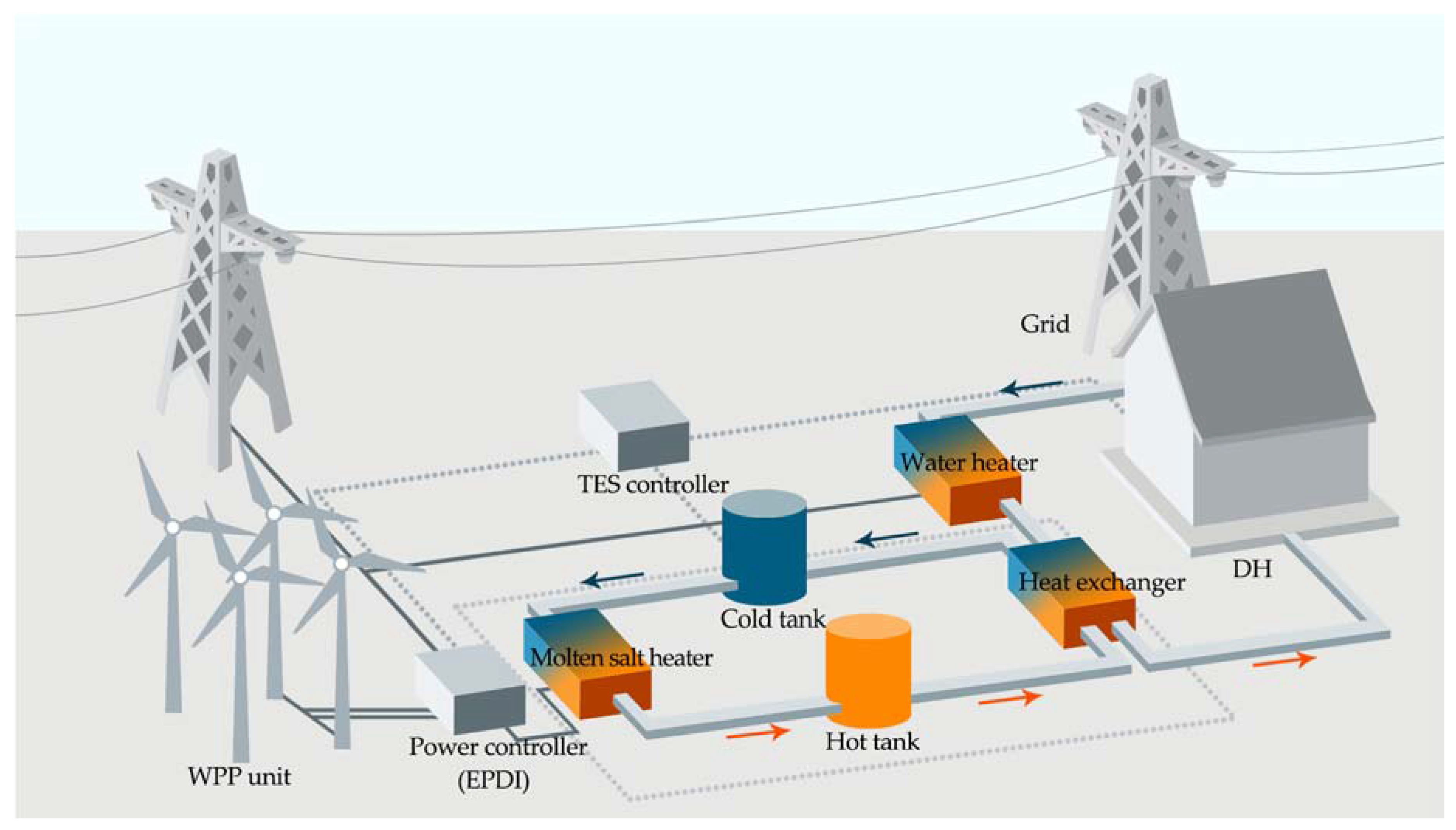
The complete WTES system is constituted by a WPP unit, a power controller (acting as an EPDI), two heaters (water heater and molten salt heater), a two-tank TES system, a heat exchanger (HE), a DH circuit and a TES controller. Typical system structure is shown in Figure 1.
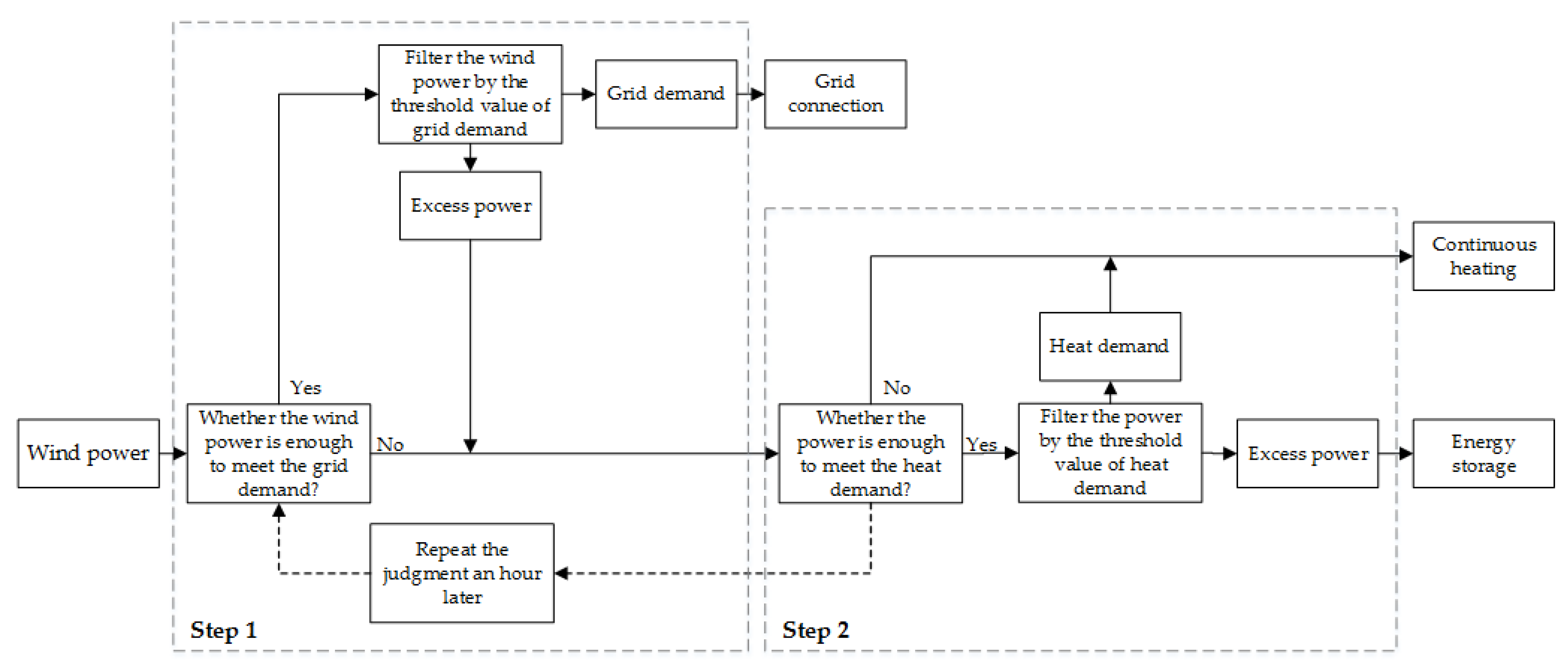
The electrical power obtained from wind fluctuates with the wind speed. Without the aid of energy storage, the wind power output cannot match the grid demand, the EPDI may curtail the excess and insufficient generation from the grid, resulting in energy rejection. The considered integrated system aims to use the cheap and rejected wind power to achieve the heat demand of users, therefore improving the utilization of wind energy. The power controller makes the decision of whether to supply and turn on the charge mode. Two-step control is applied in the power controller, the first step control is to judge whether or not the output electrical power will match the grid demand. If the output power is equal the grid demand, it will be connected to the grid. If the output power is larger than the grid demand, the excess power will be filtered out from the grid input by the power controller. Once the output power is not enough to meet the grid demand, the power controller will disconnect the insufficient power from the grid and make judgement an hour later (refer to the operational constraint applied in flexible small and medium-sized reactor according to reference [39]). The power controller can carry on the confluence of the filtered and disconnected electrical powers. The second step control is to divide the confluent power into two parts by the heat demand of DH. One is used for full-time continuous heating and the other one is used for TES. If the confluent power is equal to or below the heat demand, it will be used to heat the water of the heating loop directly (continuous heating) in a water heater. If the confluent power exceeds the heat demand, the excess part will be stored in the direct two-tank TES system and come into use when the continuous heating power cannot meet the heat demand. The electric and heat demands are changeable due to the living style of humans and climate change. The control scheme described above is summarized by the flow chart in Figure 2.
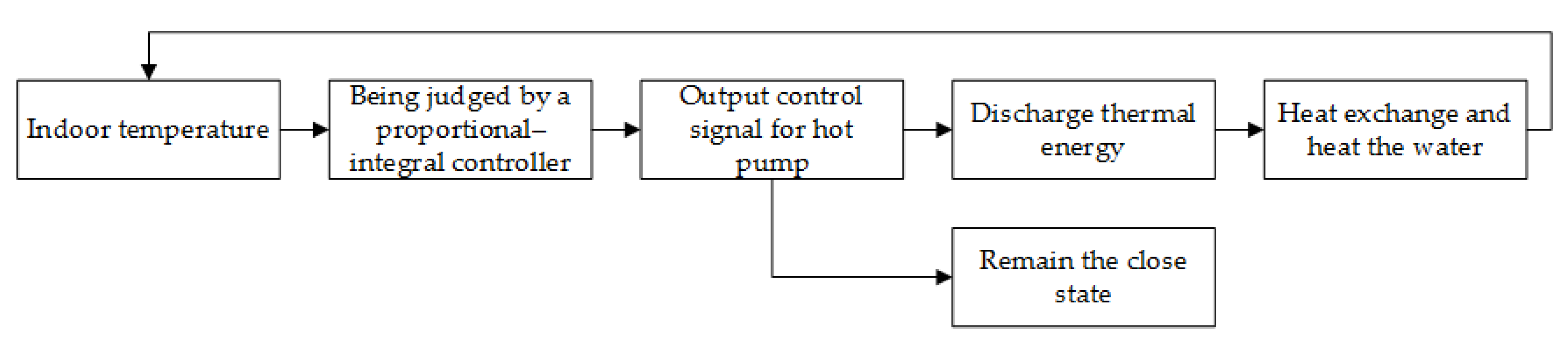
The heat demand is proportional to the temperature difference between the outdoor and indoor temperatures of the user side. The TES system is designed to keep the indoor temperature heated to a normalized comfort temperature (NCT) by the method of charging and discharging. During most of the heating period, continuous heating power can satisfy the heating demand. However, the indoor temperature of the user side may drop below the NCT when the wind power is lower than heat demand. Under this scenario, the TES system can smooth or eliminate the temperature fluctuations by releasing the stored thermal energy to reheat the circulating water. A proportional-integral (PI) controller is used here to achieve the cooperative control between TES and DH. The control scheme for the discharge sector is summarized in Figure 3.
As shown in Figure 1, The TES system is placed between the WPP and DH network. The electric heater for circulating water heating and the molten salt-water heat exchanger are put together in a series. The cold molten salt is heated by the excess wind power with the electrical molten salt heater and then stored in the hot storage tank. When there is a demand of heating supply, the hot molten salt is pumped out from the hot storage tank to discharge thermal energy through the molten salt-water heat exchanger. After heat exchanging, the cooled molten salt returns to the initial temperature and flows back to the cold storage tank. The detailed design and operating parameters of the integrated WTES system are listed in Table 1.
3. Mathematical Model
System control and system performance prediction are two of the most important goals of system simulation. The numerical results can be helpful to the optimal design of an integrated system. In this section, a model library developed with Modelica in Dymola simulation platform and the main components within the model library for system modeling will be presented.
3.1. Modelica Model Library
Modeling and simulations are very useful for engineering design, operating control and optimization of a complex heterogeneous physical system like WTES system. Besides, they play very important roles in checking, validating and improving the system performances. Modelica is a non-proprietary, object-oriented, multi-domain and equation-based language, it is very suitable for modeling and simulation of systems.
Recently, many studies on the modeling and simulation of renewable energy systems have been done with Modelica. Particularly, it has been adopted for the dynamic performance analysis of WPPs and TES systems for CSP plants. Eberhar et al. [40] developed an open source Modelica library to model the overall behavior of a WPP. Petersson et al. [41] implemented the model of a small WPP with Dymola and tested the optimization and control of the power output. Hefni et al. [42,43] established a Modelica-based generic library for the thermodynamic community, the library was mainly used to study some characteristics of CSP plant. Zaversky et al. [44] simulated the transient responses of a typical active indirect two-tank TES system. Faille et al. [45] dealt with the development of a control design model for a 1 MW Solar Tower equipped with a heat storage facility. These studies can be used as reference for the modeling and simulation of the designed integrated system. In the present modeling efforts, a new model library named WindEnergyStorage is developed and intends to be used for the numerical analysis of WPP systems, TES systems, DH systems and other related energy sectors.
3.2. Components Models
3.2.1. Wind Power Unit Module
In a wind power unit, the kinetic energy of wind is converted to electric energy. The unit module consists of four main model components: the wind source model, the wind turbine model, the gearbox model and the generator model. There are many methods for modeling the wind source, the simplest way is to capture the wind speed from a real wind farm. In a single wind power unit, wind energy is extracted from wind by the combined work of blades, rotor and pitch, which together make up the wind turbine model. Then, the energy will be passed to a generator via a gearbox. The gearbox connects the turbine with the generator and increases the low rotating speed in the wind turbine into a higher value; the generator is coupled to the high-speed side of the gearbox and transforms the mechanical energy into electricity.
The kinetic power from the wind is given by the following equation:
where ρ is the density of air, S is the effective area swept by the blades and v is the input wind speed.
According to Betz’s law, the actual power conversion efficiency of a wind turbine is always less than a limit ratio of 16/27 () [46]. Thus, the actual power converted by wind turbine is
where is the performance coefficient of wind turbine, and the maximum will not be greater than 0.593.
If the angular movement of airstream is taken into account, the performance coefficient can be described by nonlinear functions of the pitch angle of blades and the tip speed ratio of the wind turbine, and modeled by the empiric Equations (3) and (4) [47,48]:
and
where β represents the pitch angle and the tip speed ratio λ is defined as the weighted ratio of the tangential speed and the wind speed:
Besides, C1–C6 are experimental coefficients following to the reference [47], ωW and R are the angular velocity and the radius of the turbine blades, respectively.
The transmission mechanism among the wind turbine, gearbox and generator is described as the followed kinetic equation:
where parameters J and τ represent the moment of inertia and torque and the subscripts W and G represent the wind turbine and generator, respectively. γ represents the transmission ratio in the gearbox. Each of the models is connected by a torque signal depending on the generated wind power of wind turbine and the transmission ratio of gearbox. The output power of generator is calculated as:
where ωG represents the angular velocity of generator. The relationship between wind turbine and generator are described by the Equations (8) and (9):
In addition, there are cut in and cut out velocities which should be taken into consideration for production and safety reasons, no electric power will be produced if the wind speed goes out of the range defined by the cut in and cut out velocities.
3.2.2. Heater Modules
The most common heating equipment for liquid medium is the electric boiler. In this work, both two electric devices (water heater and molten salt heater) are simplified as one-dimensional models. The fluids enter the heaters and absorb heat via a heat-conducting model. The heat flow rate of the heat-conducting model is calculated as:
where the Wt represents the heat flow rate, ηe-t is the efficiency of thermo-electrical conversion, Pe is the electric power input (continuous heating power and charge rate) of the electric heater, represents the mass flow rate of fluid, cpf is the specific heat of fluid and ΔTf is the fluid temperature difference between outlet and inlet.
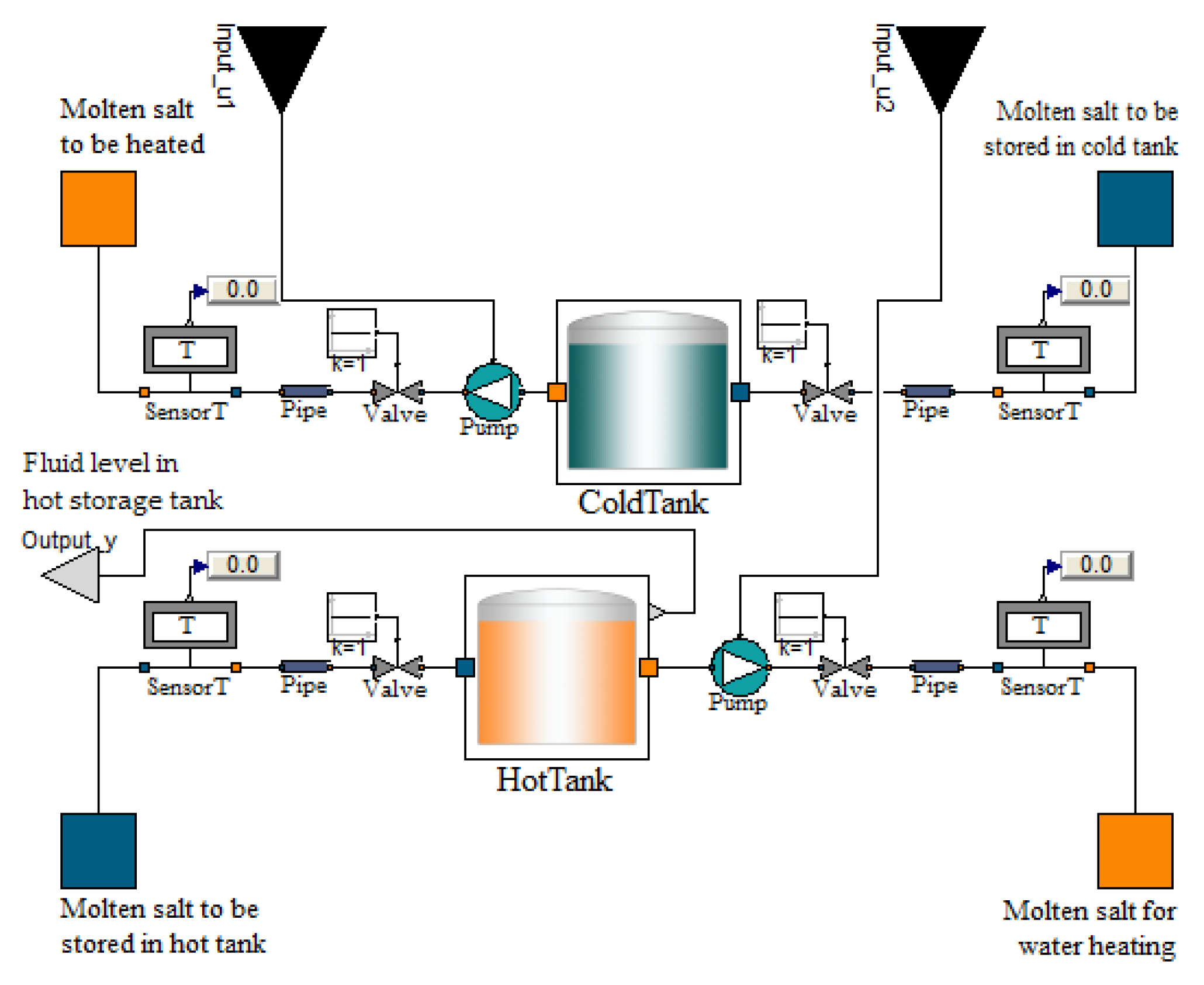
3.2.3. Two-Tank Storage Module
As one of the most important sectors of the integrated system, the two-tank storage module includes two storage tanks (a hot tank and a cold tank), two pumps, several temperature sensors, control valves, pipes and function connectors. The schematic of this storage module is presented in Figure 5. The overall module will be controlled by the TES controller module through the connectors Input_u1, Input_u2 and hot tank fluid level output (Output_y), among which the fluid level of the hot tank is involved in the control with the limited maximum and minimum levels (sum of initial fluid levels in cold and hot tanks; 0). The monitoring of inlet and outlet temperatures of the hot and cold tanks can be achieved by the temperature sensors located at each side of tanks.
Unlike the single-tank system and phase change material storage system, the two-tank storage system achieves the goals of charging and discharging with little attention to the temperature distribution of the fluid in tanks. So, for the sake of simplicity, temperature distributions in the storage tanks are ignored.
The fluid flow components in this module are developed as one-dimensional dynamic models, mainly based on a generic set of equations of the conservation of mass, energy and momentum:
where ρ, , h and p are, respectively, the density, mass flow rate, specific enthalpy and pressure of the fluid (molten salt), A is the cross-sectional area of the component for fluid, g is the constant of gravity, ΔQ denotes any other energy attached, z and F are respectively set for the elevation and sum of forces. The subscript x is used to represent the position along the flow direction of the components, and Δx is the quantities of the position variation. Besides, the fluid internal specific energy ux in Equation (13) is given by
3.2.4. Heat Exchanger Module
The heat exchanger is applied to realize the heat transfer between molten salt and water. The one-dimensional model, which is suitable for transient response analysis, is employed to reflect the temperature variation of both sides of heat transfer walls. The outlet temperature of one side in the heat exchanger is determined by the inlet temperature, the mass flow rate of the HTF, the specific heat of the HTF and the heat transfer rate. Besides, the exchange effectiveness is taken into consideration. The physical processes can be described by equations
where and are the mass flow rates of molten salt and water, cps and cpw respectively denote the specific heat of molten salt and water, Ts,in, Ts,out, Tw,in and Tw,out respectively represent the inlet and outlet temperatures of molten salt and water, Ws and Ww are the heat transfer rate of molten salt and water, ηHE is the efficiency of the heat exchange between two sides.
3.2.5. Heating Loop Module
In this module, the loop provides heat to the space of the user side through a heat exchanger. The physical process is achieved by a convection heat transfer model. The employed correlation for the model is given by:
where WDH is the heat transfer rate, k is the heat transfer coefficient, ADH is the heat transfer surface and Tw is the inlet temperature of the heat exchanger, and Ta is the temperature of the indoor air.
3.2.6. Controller Modules
The air temperature of the user side is kept to the set value NCT by the means of two system level controllers: the power controller and the TES controller.
The power controller is used to divide the wind power into three branches with electric load and heat load, respectively, for the use of electrical power supply, continuous heating and temperature compensation.
The charge and discharge processes of the thermal storage system are achieved by a TES controller. The TES controller is to control the outlet flow rates of cold and hot storage tanks. The input power for each heating loop, the feedback temperature of the user side and the fluid level are key criteria for the charge and discharge control processes. The pumps use the calculated parameters to modulate the outlet mass flow rates in order to meet the set point NCT. If the input power of salt heater is greater than zero, the charge mode is turned on. Conversely, if the input power of salt heater is zero or the hot storage tank is full load, the charge mode will be turned off.
The outlet mass flow rate of cold tank pump is defined as:
where the Wt represents the heat flow rate and ΔTf (calculated as 273 K) is the difference between the temperatures of cold and hot storage tank. The control of the outlet mass flow rate of the hot tank pump is governed by a PI controller which can maintain the feedback air temperature of the user side within the desired range, the pump will be turned on whenever the feedback temperature of the DH loop falls below NCT.
The actual utilization of total available wind energy of the system is defined as:
where EW is the total available wind energy, Eu is the sum of the utilized energy. EDH and EES are the portions of the wind energy which are used for DH and electricity supply, and EN is the net TES at the end of the operation. EW, EDH, EES and EN are calculated as:
where Echarge and Edischarge are the charge and discharge energies. PW, PCH, PES, Pcharge and Pdischarge respectively represent the total generated wind power, the continuous heating power, the electricity supplying power, the charge power and the discharge power. Td is the test duration.
Thus, the total wind rejected power is defined by the equation:
The completion rate of electric power supply and DH are respectively defined as:
where the EED and ETD respectively represent the electrical and thermal energy demand. EED and ETD are defined as:
PED and PTD are the electric load and heat load, respectively.
3.3. Model Validation
The validation of the TES model developed in Section 3.2 is performed by comparing its numerical results with the experimental results obtained from the work of Peiró et al. [32]. The two loops, including HTF loop and TES loop, are used to carry out the experiment of a smaller scale indirect two-tank MSTES system. Synthetic thermal oil (Therminol VP-1) and molten salt (Solar Salt) were respectively employed as the HTF and the TES medium in these two loops. The charge and discharge processes were implemented and tested.
The parameters, such as initial temperature, the flow rate of fluid, thermal properties of heat transfer and heat storage media, etc. are adopted to accommodate the experimental setup. The simulation model is developed according to the experimental facility. The experimental conditions are tabulated in Table 2.
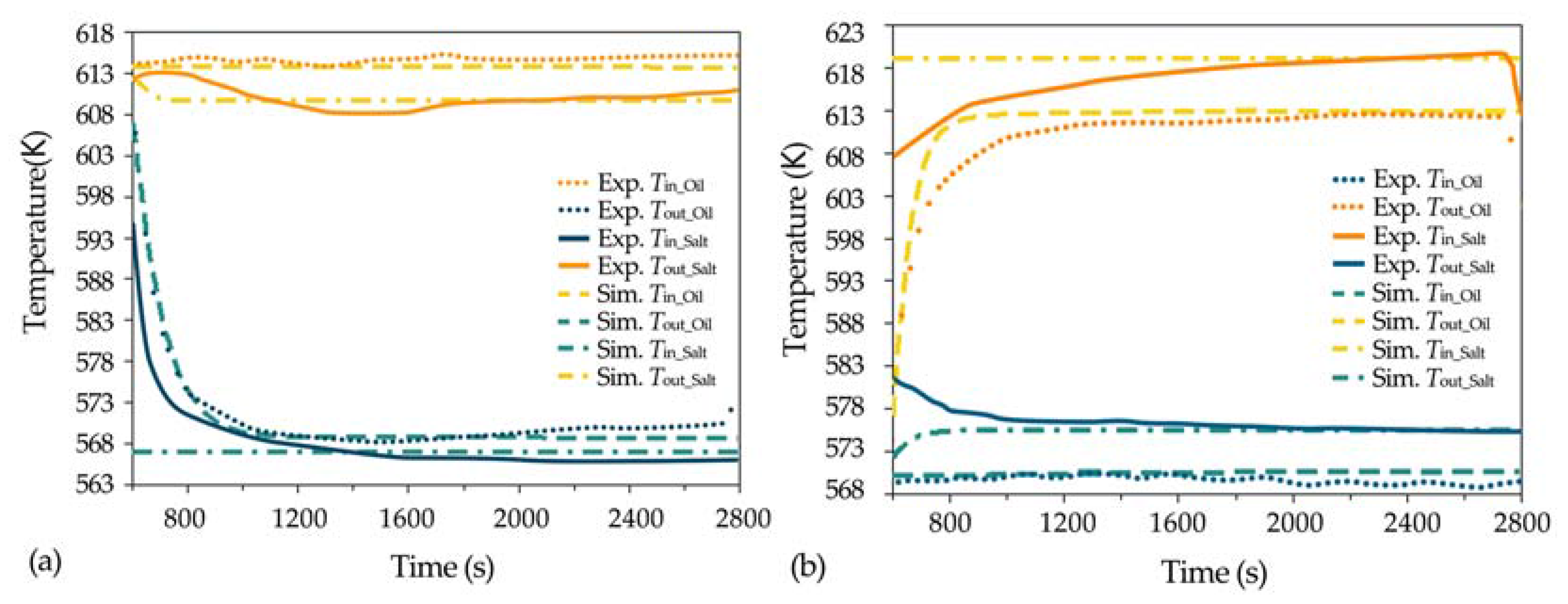
Figure 6 shows the inlet and outlet temperature evolutions in both HTF and TES sides of the heat exchanger in the indirect two-tank MSTES system during a charge and discharge process, respectively. The dotted and solid lines represent the temperatures of synthetic thermal oil and molten salt in the reference experiment, respectively. In our simulation work, the dashed lines represent the temperatures of synthetic thermal oil, and the dash-dot lines represent the temperatures of molten salt.
From Figure 6, there are two differences between the experimental results and numerical results. The first one is that the gradual changes of inlet molten salt temperatures can be observed in the beginning of both experimental charge and discharge processes, the change during the charge process is from a higher temperature to the design value, and the change during the discharge process is from a lower temperature to the design value. Referring to the explanation of the literature [32], this is because an electrical tracing system is installed along the piping of the molten salt loop to help maintain the molten salt pipes at a desired temperature and avoid solidification problems. Another difference is the small discrepancy between the outlet temperatures in the molten salt side of the experiment and numerical test. Gradual changes are visible in the beginning of both numerical charge and discharge processes. The outlet temperatures of the molten salt in the beginning of the running processes are close to the inlet temperatures of synthetic thermal oil, unlike the values in the experiment. This gradual change is due to the temperature front propagation which is caused by the initial temperature settings and the running process of the model. During the run time, the synthetic thermal oil is flowing continuously, and the molten salt only flows during the charge and discharge processes; therefore, the molten salt outlet temperature is affected by the temperature of the synthetic thermal oil side.
When the systems reach a dynamic balance state, the numerical results are observed to agree well with the experimental results within the consideration of uncertainty in heat transfer coefficients, heat loss of real experiment apparatus and measurement errors. The validation work proves that the TES system model and its components models are reliable to be taken as an evaluation basis. Furthermore, the model library can be flexibly applied in any related system modeling and simulation works.
3.4. Model Assumptions
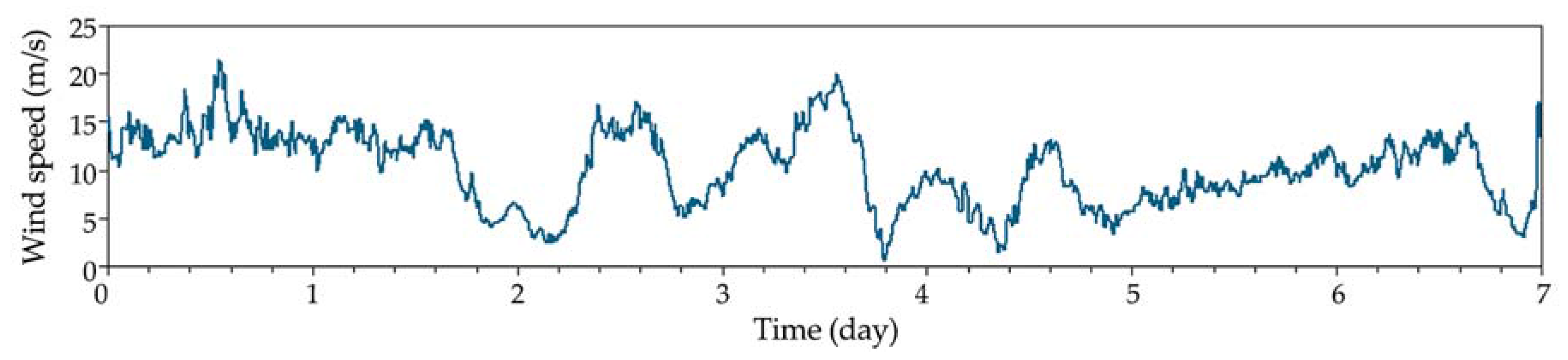
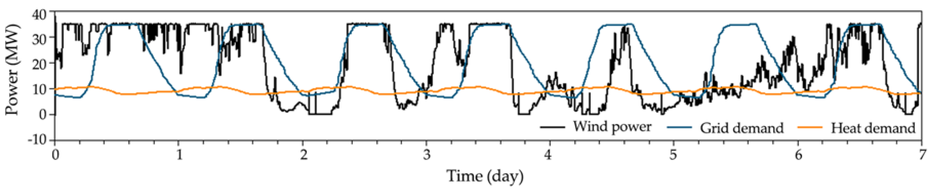
The variation of wind speed acquired from the reference [40] is shown in Figure 7, the time interval of the data is 10 min. The WPP system is assumed to contain ten wind turbines with rated capacity of 3.5 MW. The cut in and cut out velocities are 4 m/s and 25 m/s, respectively. Thus, the total power generation of the wind farm can be calculated. The results are shown in Figure 8. For simplicity, the variations of (1) the outdoor temperature of user side acquired from the reference [49] and (2) grid demand acquired from the reference [50] are copied to seven-day diurnal curves and assumed to be identical every single day. Besides, the grid demand profile is specified such that the maximum grid demand is equal to the rated capacity of the wind farm (35 MW). The grid demand and heat demand (calculated ignoring the heat exchange between indoor and outdoor) are also plotted in Figure 8.
4. Results and Discussion
4.1. Operation and Performance of the Integrated System
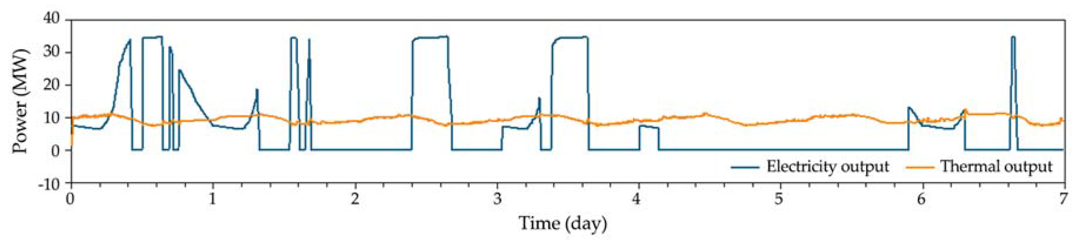
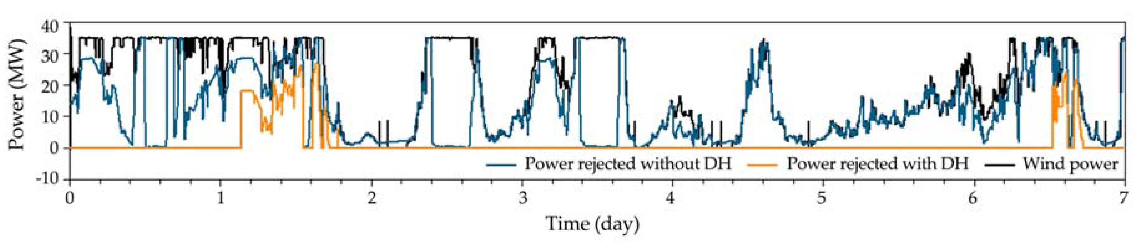
In this section, a one-week simulation of the WTES system is presented. Figure 9 shows the actual electrical and thermal outputs of the WTES system. It is observed that the electricity output can meet the grid demand for several short periods and remain insufficient during the rest of the periods. This is caused by the nature of the generation of the WPP system, whose output profile is unmatched with the current grid demand. This leads to a great amount of wind energy rejection (65.2%) during the period when the WPP system is not equipped with a TES (referring to the Figure 10). With the consumption of the DH system, most of the rejected wind power is utilized as thermal power. As shown in Figure 10, the wind energy rejection is largely reduced when WTES is applied. However, a small amount of wind energy (8.5%) is still rejected, due to the limited capacity of the TES system. It is also observed that the heat demand can be satisfied all the time, in which case the indoor temperature of the user side is in a relatively stable range (around NCT).
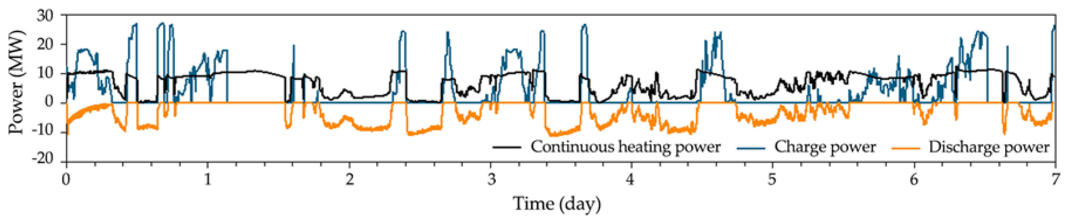
Figure 11 shows the energy flow of the DH system. The heat load acts as the threshold here and divides the rejected wind power into two parts: continuous heating and TES. During the periods that the heat demand can be satisfied by directly consuming the rejected power, the variable excess wind power is charged into the TES as thermal energy for later use. When the rejected wind power cannot meet the heat demand, the TES discharges thermal energy as a supplement to maintain the desired thermal energy supply.
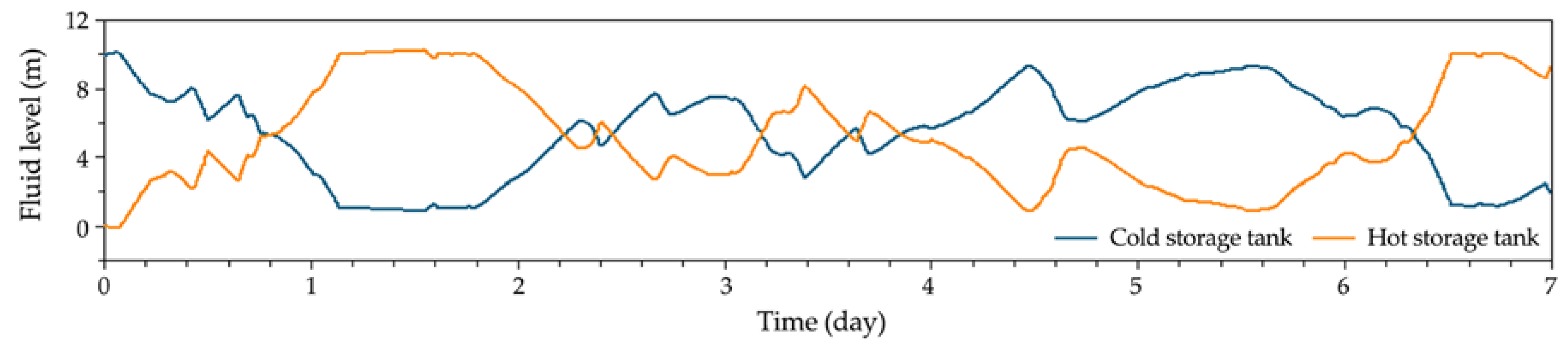
Figure 12 describes the variations of fluid levels in the cold and hot storage tanks, respectively. It is observed that the fluid level changes as the charges and discharges processes. As can be seen in Figure 12, the fluid level of the hot storage tank is maintained at the maximum (10 m) over several periods of time (1.10–1.58 d, 1.60–1.79 d and 6.50–6.65 d and 6.68–6.74 d). This corresponds to the wind energy rejection (shown by the orange line in Figure 10) due to the limit of the tank size.
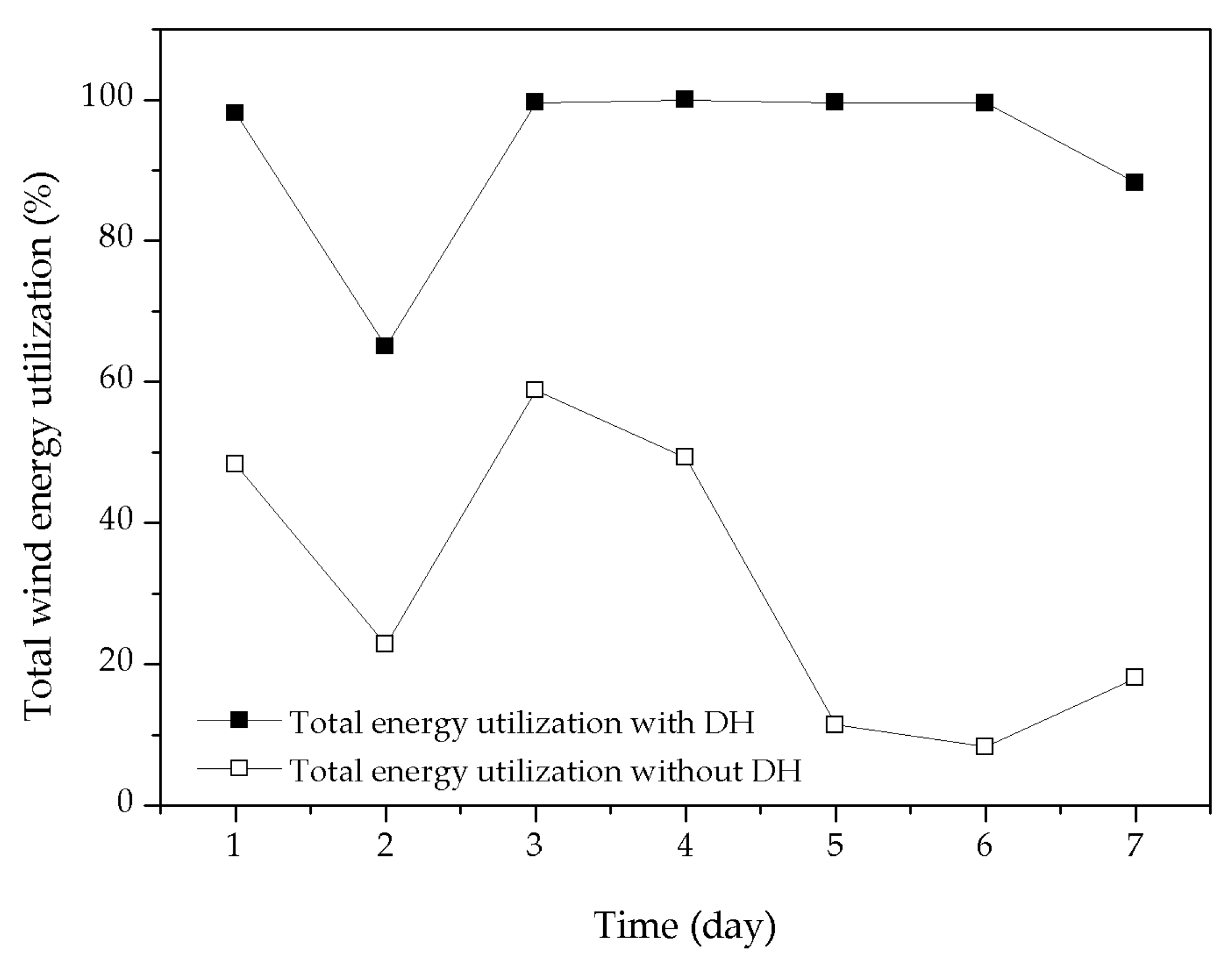
Figure 13 illustrates the comparison of total available wind energy utilization of the system between using and not using DH and TES. The total energy utilization is defined by Equation (21). The result shows that the daily utilizations of the WPP system (without using DH and TES) keep at a very low level (from 8.3% to 58.8%), while the daily utilizations of the WTES system are much higher (from 65.0% to 100.0%). Particularly, the actual total energy utilization of the WTES system reaches 100% in day 4. It is worth noting that during the periods (days 2, 5, 6 and 7) when the wind resources are too poor to match the electric energy demand, the DH system together with the TES system consume a great part of the wind power rejection. This significantly increases the energy utilization of the system. The actual wind energy utilization during the seven-day operation increases from 34.9% to 83.7% by applying DH and TES. Detailed simulation results of the operation performance are tabulated in Table 3.
4.2. The Influence of the System Configuration on the Performance of the Integrated System
In this section, parametric analysis is conducted to investigate the influence of the system configuration on the performance of the integrated WTES system. Different storage tank sizes (6 m, 8 m, 10 m, 12 m and 14 m in diameter) and areas of DH (30,000, 50,000, and 70,000 m2) are adopted.
Table 4 provides the performance variations of the WTES system with different storage tank diameters. From the observations in Table 4, it is found that the heat demand cannot be completely met when the storage tanks have a diameter below 8 m. This provides a design reference for the scale of TES. The net TES during a one-week operation is observed to increase with the diameter of the storage tanks. Accordingly, the rejected wind energy decreases, because TES with a larger scale can provide larger capacity to utilize the power rejection for later use. From the comparison between systems using or not using DH to utilize the wind power rejection, it is found that the wind energy rejection significantly drops (around 1–2 orders of magnitude) when a WPP system employs a DH system. Accordingly, the energy utilization largely increases (around 2–3 times), and reaches a satisfying level (over 85%).
Table 5 gives the simulation results of the system performances under various DH scales, using a fixed grid demand and TES scale (10 m in diameter). It is found that the heat demand can be completely satisfied when the heating area is 30,000 and 50,000 m2. When the heating area increases to 70,000 m2, the completion rate of DH drops below 100%. However, such a great heating area (heat demand) significantly contributes to the reduction of the wind energy rejection, which results in a much higher total energy utilization of the system. It can be predicted that larger TES scales (for instance, using storage tanks with a diameter of 12 m and 14 m) may afford a complete heat supply for such a heating area. However, the scale of TES system is also limited by economic factors, which will be discussed in our future work.
5. Conclusions
In the present study, a WPP integrated with TES for DH was proposed to improve the utilization of wind energy, especially when the wind power rejection occurs in winter days. The feasibility of the solution was taken into account. Details in system operation and controlling process were described for the integrated WTES system. A generic model library and a one-dimensional system model of the integrated system were developed with the object-oriented programming language Modelica based on the Dymola simulation platform. The validation work of the main components of the TES module against experimental results was conducted. The results proved that the component models are reliable. The dynamic performances of the considered system were analyzed by using the system model based on a seven-day operation. Wind energy saving dispatch was given under the operation mode. The fluid levels in both cold and hot storage tanks were plotted. The effects of different system configurations on the performance of the integrated system were also analyzed. The main conclusions of the WTES system are summarized as follows:
- (1)
- The seven-day simulation results showed that the daily utilization of wind energy of the WTES system is much higher than that of the WPP system (without DH and TES). Meanwhile, the normal operation of the WTES system is under a simple and automatic control scheme, by which the electricity supplying and the DH form integrated dispatching and command.
- (2)
- The integrated system with a larger scale of TES can provide larger capacity to utilize the rejected wind energy, thus resulting in a higher total energy utilization. Parametric analysis reveals that the WTES system performance in the case of a given scale of the wind farm mainly depends on the configuration of the TES system and heat demand from users. The optimal design of the system can be carried out by giving the actual conditions of each wind farm and user demand.
- (3)
- In summary, the integrated WTES system is considered to be effective on enhancing the utilization of wind energy under great wind rejection.
Acknowledgments
This paper is supported by the Chinese TMSR Strategic Pioneer Science and Technology Project (No. XD02001003).
Author Contributions
Chang Liu developed the frame work of the paper and did the numerical simulations. Chang Liu and Bing-Chen Zhao prepared the manuscript. Mao-Song Cheng and Zhi-Min Dai reviewed the manuscript and made revision suggestions.
Conflicts of Interest
The authors declare no conflict of interest.
Nomenclature
| Notations | |
| A | Cross-sectional area of the flow component (m2) |
| ADH | Heat transfer surface (m2) |
| cp | Specific heat (J/kg/K) |
| C | Experimental coefficients |
| CP | Performance coefficient of wind turbine |
| E | Energy (MWh) |
| F | Friction force (kg/m/s2) |
| g | Constant of gravity (m/s2) |
| h | Specific enthalpy (J/kg) |
| J | Moment of inertia (kg∙m2) |
| k | Heat exchanger coefficient (W/m2/K) |
| Mass flow rate (kg/s) | |
| p | Pressure (Pa) |
| P | Power (W) |
| Pe | Electrical power input of electric heater (W) |
| PW | Wind power generated by wind turbine (W) |
| ΔQ | Energy variation (J) |
| R | Radius of wind turbine blade (m) |
| S | Effective area swept by wind turbine blades (m2) |
| t | Time (s) |
| T | Temperature (K) |
| Td | Test duration (s) |
| ΔTf | Temperature difference of fluid (K) |
| u | Internal specific energy of fluid (J/kg) |
| v | Wind speed (m/s) |
| WDH | Heat transfer rate of user side in DH sector (W) |
| Ws | Heat transfer rate of molten salt (W) |
| Wt | Heat flow rate (W) |
| Ww | Heat transfer rate of water (W) |
| x | Position (m) |
| Δx | Position variation (m) |
| z | Elevation (m) |
| Subscripts | |
| a | Air |
| c | Cold tank |
| CH | Continuous heating |
| charge | Charge mode |
| DH | District heating |
| discharge | Discharge mode |
| e | Electric |
| e-t | Thermo-electric conversion |
| ED | Electrical energy demand |
| ES | Electrical power supply |
| f | Fluid |
| G | Generator |
| HE | Heat exchanger |
| in | Inlet |
| N | Net storage (thermal energy) |
| out | Outlet |
| r | Power rejected |
| s | Molten salt |
| S | Storage |
| t | Thermal energy |
| TD | Thermal energy demand |
| u | Utilizing |
| w | Water |
| W | Wind turbine |
| Greek symbols | |
| β | Pitch angle (rad) |
| γ | Transmission ratio |
| δ | Completion rate (%) |
| η | Efficiency (%) |
| ζ | Total available energy utilization (%) |
| λ | Tip speed ratio of wind turbine blade |
| ρ | Density of air (kg/m3) |
| τ | Torque (N∙m) |
| ω | Angular velocity of turbine (rad/s) |
| Abbreviations | |
| CSP | Concentrating solar power |
| DH | District heating |
| EPDI | Electric power dispatching institution |
| HE | Heat exchanger |
| HTF | Heat transfer fluid |
| MSTES | Molten salt TES |
| NCT | Comfort temperature of norm |
| PI | Proportional-intergral |
| TES | TES |
| WPP | Wind power plant |
| WTES | Wind-TES system |
References
- Zhao, X.; Li, S.; Zhang, S.; Yang, R.; Liu, S. The effectiveness of China’s wind power policy: An empirical analysis. Energy Policy 2016, 95, 269–279. [Google Scholar] [CrossRef]
- Global wind Energy Outlook Scenarios. Global Wind Energy Outlook 2016; Fried, L., Shukla, S., Eds.; Global Wind Energy Council: Brussels, Belgium, 2016; pp. 15–30. [Google Scholar]
- Albadi, M.H.; El-Saadany, E.F. Overview of wind power intermittency impacts on power systems. Electr. Power Syst. Res. 2010, 80, 627–632. [Google Scholar] [CrossRef]
- Zhang, Y.; Tang, N.; Niu, Y.; Du, X. Wind energy rejection in China: Current status, reasons and perspectives. Renew. Sustain. Energy Rev. 2016, 66, 322–344. [Google Scholar] [CrossRef]
- Cochran, J.; Miller, M.; Zinaman, O.; Milligan, M.; Arent, D.; Palmintier, B.; O’Malley, M.; Mueller, S.; Lannoye, E.; Tuohy, A.; et al. Flexibility in 21st Century Power Systems; National Renewable Energy Lab.: Golden, CO, USA, 2014. [Google Scholar]
- Jiang, Y.; Xu, J.; Sun, Y.; Wei, C.; Wang, J.; Ke, D.; Li, X.; Yang, J.; Peng, X.; Tang, B. Day-ahead stochastic economic dispatch of wind integrated power system considering demand response of residential hybrid energy system. Appl. Energy 2017, 190, 1126–1137. [Google Scholar] [CrossRef]
- Lund, P.D.; Lindgren, J.; Mikkola, J.; Salpakari, J. Review of energy system flexibility measures to enable high levels of variable renewable electricity. Renew. Sustain. Energy Rev. 2015, 45, 785–807. [Google Scholar] [CrossRef]
- Sullivan, P.; Short, W.; Blair, N. Modelling the benefits of storage technologies to wind power. In Proceedings of the American Wind Energy Association Wind Power 2008 Conference, Golden, CO, USA, 1–4 June 2008. [Google Scholar]
- Díaz-González, F.; Sumper, A.; Gomis-Bellmunt, O.; Villafáfila-Robles, R. A review of energy storage technologies for wind power applications. Renew. Sustain. Energy Rev. 2012, 16, 2154–2171. [Google Scholar] [CrossRef]
- Yuan, Y.; Zhang, X.; Ju, P.; Fu, Z. Determination of economic dispatch of wind farm-battery energy storage system using genetic algorithm. Int. Trans. Electr. Energy Syst. 2014, 24, 264–280. [Google Scholar] [CrossRef]
- Zahedi, A. Sustainable power supply using solar energy and wind power combined with energy storage. Energy Procedia 2014, 52, 642–650. [Google Scholar] [CrossRef]
- Monroy, C.A.S.; Christie, R.D. Energy storage effects on day-ahead operation of power systems with high wind penetration. In Proceedings of the North American Power Symposium 2011, Boston, MA, USA, 4–6 August 2011. [Google Scholar]
- Amrouche, S.O.; Rekioua, D.; Rekioua, T.; Bacha, S. Overview of energy storage in renewable energy systems. Int. J. Hydrogen Energy 2016, 41, 20914–20927. [Google Scholar] [CrossRef]
- Zhang, Y.; Ding, W. Increasing Wind Power Consumption & Absorbability, Solving Grid Connection Issue by Use of Thermal Energy Storage Technology. In Proceedings of the Chinese Society for Electrical Engineering Annual Meeting 2012, Beijing, China, 21–24 November 2012. [Google Scholar]
- Li, G. Sensible heat thermal storage energy and exergy performance evaluations. Renew. Sustain. Energy Rev. 2016, 53, 897–923. [Google Scholar] [CrossRef]
- Tyner, C.E.; Sutherland, J.P.; Gould, W.R. Solar Two: A Molten Salt Power Tower Demonstration; Sandia National Laboratories: Albuquerque, NM, USA, 1995. [Google Scholar]
- Pacheco, J.E.; Reilly, H.E.; Kolb, G.J.; Tyner, C.E. Summary of the Solar Two Test and Evaluation Program; Sandia National Laboratories: Albuquerque, NM, USA, 2000. [Google Scholar]
- Hasnain, S.M. Review on sustainable thermal energy storage technologies, part I: Heat storage materials and techniques. Energy Convers. Manag. 1998, 39, 1127–1138. [Google Scholar] [CrossRef]
- Herrmann, U.; Kelly, B.; Price, H. Two-tank molten salt storage for parabolic trough solar power plants. Energy 2004, 29, 883–893. [Google Scholar] [CrossRef]
- Parrado, C.; Marzo, A.; Fuentealba, E.; Fernández, A.G. 2050 LCOE improvement using new molten salts for thermal energy storage in CSP plants. Renew. Sustain. Energy Rev. 2016, 57, 505–514. [Google Scholar] [CrossRef]
- Glatzmaier, G. Developing a Cost Model and Methodology to Estimate Capital Costs for Thermal Energy Storage; NREL/TP-5500-53066; National Renewable Energy Laboratory: Golden, CO, USA, 2011. [Google Scholar]
- Okazaki, T.; Shirai, Y.; Nakamura, T. Concept study of wind power utilizing direct thermal energy conversion and thermal energy storage. Renew. Energy 2015, 83, 332–338. [Google Scholar] [CrossRef]
- Xinhuanet. State Grid Corporation of China Published the “White Paper for Promoting the Development of New Energy (2016)”. Available online: http://news.xinhuanet.com/2016-03/11/c_1118307562.htm (accessed on 11 March 2016).
- State Grid Corporation of China. The Means to Capture the Wind. Available online: http://www.sgcc.com.cn/xwzx/gsyw/2017/03/338555.shtml (accessed on 16 March 2017).
- ZhongTouYiXing New Energy Investment Co. Ltd. Zhong Tou Yi Xing New Energy Investment Corporation Employs the Electrical Heated Molten Salt Thermal Energy Storage Technology for Domestic Heating. Available online: http://www.ztyxxny.com/newsdetail/91.html (accessed on 22 April 2016).
- Xinhuanet. The Technology of Molten Salt Thermal Energy Storage by Utilizing Valley Electricity for Heat Helps Realize the Heating Reform Project. Available online: http://news.xinhuanet.com/2016-01/25/c_1117885895.htm (accessed on 25 January 2016).
- Martin, M.; Thornley, P. The Potential for Thermal Storage to Reduce the Overall Carbon Emissions from District Heating Systems; The Tyndall Centre: Tyndall Manchester, UK, 2012; pp. 4–8. [Google Scholar]
- Arabkoohsar, A.; Andresen, G.B. Design and analysis of the novel concept of high temperature heat and power storage. Energy 2017, 126, 21–33. [Google Scholar] [CrossRef]
- Lidegaard, M. District heating-Danish and Chinese Experience; Danish Board of District Heating & Danish Energy Agency: Frederiksberg, Denmark, 2013; pp. 5–14. [Google Scholar]
- Wu, Y.; Zhang, X.; Wang, H.; Sun, J. Molten salt heat storage and supply technology based on heating using abandoned wind power, PV power or off-peak power. Sino-Glob. Energy 2017, 22, 93–99. [Google Scholar]
- Tian, Y.; Zhao, C.Y. A review of solar collectors and thermal energy storage in solar thermal applications. Appl. Energy 2013, 104, 538–553. [Google Scholar] [CrossRef] [Green Version]
- Peiró, G.; Gasia, J.; Miró, L.; Prieto, C.; Cabeza, L.F. Experimental analysis of charging and discharging processes, with parallel and counter flow arrangements, in a molten salts high temperature pilot plant scale setup. Appl. Energy 2016, 178, 294–403. [Google Scholar] [CrossRef]
- Li, X.; Xu, E.; Song, S.; Wang, X.; Yuan, G. Dynamic simulation of two-tank indirect thermal energy storage system with molten salt. Renew. Energy 2017, 113, 1311–1319. [Google Scholar] [CrossRef]
- Powell, K.M.; Edgar, T.F. Control of a large scale solar thermal energy storage system. In Proceedings of the 2011 American Control Conference, San Francisco, CA, USA, 29 June–1 July 2011. [Google Scholar]
- Zhao, Z.; Arif, M.T.; Oo, A.M.T. Solar thermal energy with molten-salt storage for residential heating application. Energy Procedia 2017, 110, 243–249. [Google Scholar] [CrossRef]
- Green, M.; Sabharwall, P.; Yoon, S.J.; Bragg-Sitton, S.B.; Stoot, C. Nuclear Hybrid Energy System: Molten Salt Energy Storage; INL/EXT-13-31768; Idaho National Laboratory: Idaho Falls, ID, USA, 2013. [Google Scholar]
- Ma, Z.; Glatzmaier, G.C.; Kutscher, C.F. Thermal energy storage and its potential applications in solar thermal power plants and electricity storage. In Proceedings of the ASME 2011 5th International Conference on Energy Sustainability, Washington, DC, USA, 7–10 August 2011. [Google Scholar]
- Mowers, M.; Helm, C.; Blair, N.; Short, W. Correlations between geographically dispersed concentrating solar power and demand in the United States. In Proceedings of the ASME 2010 4th International Conference on Energy Sustainability, Phoenix, AZ, USA, 17–22 May 2010. [Google Scholar]
- Shropshire, D.; Purvins, A.; Papaioannou, I.; Maschio, I. Benefits and cost implications from integrating small flexible nuclear reactors with off-shore wind farms in a virtual power plant. Energy Policy 2012, 46, 558–573. [Google Scholar] [CrossRef]
- Eberhar, P.; Chung, T.S.; Haumer, A.; Kra, C. Open source library for the simulation of Wind Power Plants. In Proceedings of the 11th International Modelica Conference, Versailles, France, 21–23 September 2015. [Google Scholar]
- Petersson, J.; Isaksson, P.; Tummescheit, H.; Ylikiiskil, J. Modeling and Simulation of a Vertical Wind Power Plant in Dymola/Modelica. In Proceedings of the 9th International Modelica Conference, Munich, Germany, 3–5 September 2012. [Google Scholar]
- Hefni, B.E.; Soler, R. Dynamic multi-configuration model of a 145 MWe concentrated solar power plant with the ThermoSysPro library (tower receiver, molten salt storage and steam generator). Energy Procedia 2015, 69, 1249–1258. [Google Scholar] [CrossRef]
- Hefni, B.E. Dynamic modeling of concentrated solar power plants with the ThermoSysPro library (Parabolic Trough collectors, Fresnel reflector and Solar-Hybrid). Energy Procedia 2014, 49, 1127–1137. [Google Scholar] [CrossRef]
- Zaversky, F.; Rodríguez-García, M.M.; García-Barberena, J.; Sánchez, M.; Astrain, D. Transient behavior of an active indirect two-tank thermal energy storage system during changes in operating mode—An application of an experimentally validated numerical model. Energy Procedia 2014, 49, 1078–1087. [Google Scholar] [CrossRef]
- Faille, D.; Liu, S.; Wang, Z.; Yang, Z. Control design model for a solar tower plant. Energy Procedia 2014, 49, 2080–2089. [Google Scholar] [CrossRef]
- Stiebler, M. Wind Energy System for Electric Power Generation; Springer: Berlin/Heidelberg, Germany, 2008; pp. 11–12. [Google Scholar]
- Heier, S. Grid Integration of Wind Energy: Onshore and Offshore Conversion Systems, 3rd ed.; John Wiley & Sons Ltd.: Chichester, UK, 2014; pp. 32–44. [Google Scholar]
- Catană, I.; Safta, C.; Panduru, V. Power optimization control system of wind turbines by changing the pitch angle. UPB Sci. Bull. Ser. D 2010, 72, 140–148. [Google Scholar]
- Shao, B.; Sun, C.; Qi, C. Building thermal characteristic simulation under heating condition. Heat. Vent. Air Cond. 2017, 47, 124–128. [Google Scholar]
- Zhang, X.; Yang, L.; He, B.; Zhang, A.; Wang, F. Calculation method of auxiliary power consumption rate for combined heating cooling and power distributed energy system. Therm. Power Gen. 2017, 46, 88–92. [Google Scholar]
Figure 1.
Structure of the two-tank wind-thermal energy storage (WTES) system.

Figure 2.
Flow chart about the control scheme in the power controller.

Figure 3.
Flow chart about the control scheme for the discharge sector.

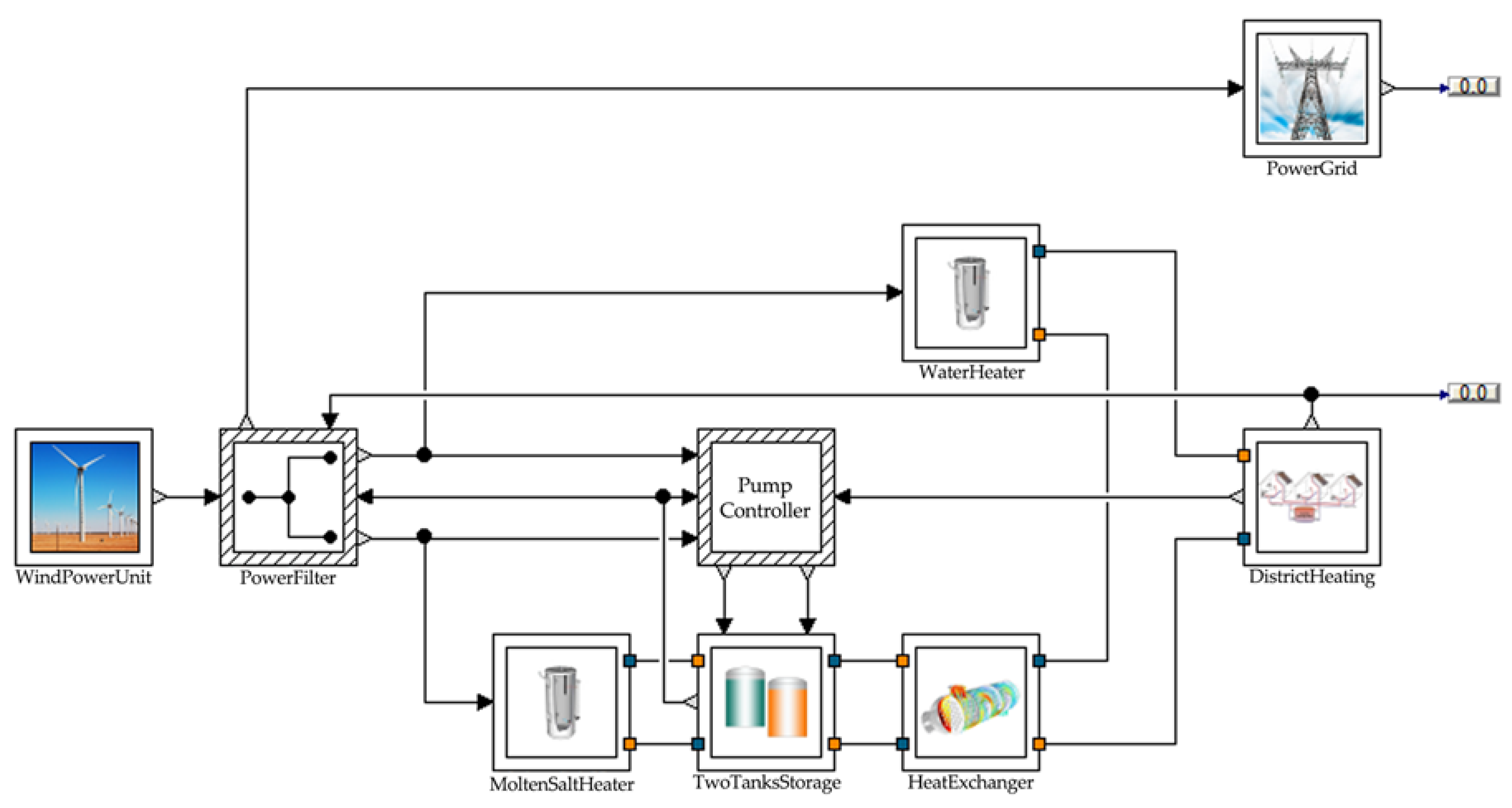
Figure 4.
Structure of the proposed WTES system model.

Figure 5.
Schematic of the two-tank storage module.

Figure 6.
Temperature evolution along time of the synthetic thermal oil and molten salt at the terminals of the heat exchanger in a counter flow arrangement during: (a) charge process; (b) discharge process.
Figure 6.
Temperature evolution along time of the synthetic thermal oil and molten salt at the terminals of the heat exchanger in a counter flow arrangement during: (a) charge process; (b) discharge process.

Figure 7.
The input wind speed over one week time range.

Figure 8.
Daily profiles of the total wind power and the loads for a typical week in a heating season.
Figure 8.
Daily profiles of the total wind power and the loads for a typical week in a heating season.

Figure 9.
Simulated results of the output electricity power and thermal power.

Figure 10.
Simulation results of the rejected wind power with and without district heating (DH).

Figure 11.
Simulated result of the input powers for storage and DH.

Figure 12.
Simulated results of the fluid levels in cold and hot molten salt storage tanks.

Figure 13.
Daily evolutions of the total wind power utilization of WPP with and without DH.


Table 1.
Design parameters of the integrated WTES system. NCT: normalized comfort temperature; HE: heat exchanger.
Table 1.
Design parameters of the integrated WTES system. NCT: normalized comfort temperature; HE: heat exchanger.
| Parameter | Unit | Value |
|---|---|---|
| Diameter of blades | m | 90 |
| Density of air | kg/m3 | 1.2 |
| Initial temperature of molten salt | K | 563 |
| Operating temperature of cold tank | K | 563 |
| Operating temperature of hot tank | K | 838 |
| Efficiency of pumps | - | 70% |
| Density of molten salt | kg/m3 | 2089.905 − 0.636 T (°C) |
| Specific heat of molten salt | J/(kg∙K) | 1443 + 0.172 T (°C) |
| Thermal conductivity of molten salt | W/(m∙K) | 1.9 × 10⁻⁴ T (°C) + 0.443 |
| Kinematic viscosity of molten salt | m2/s | −6.557 × 10⁻¹⁴ T3 (°C) + 1.05 × 10⁻¹⁰ T2 (°C) − 5.706 × 10⁻⁸ T (°C) + 1.112 × 10⁻⁵ |
| Height of cold tank | M | 10 |
| Height of hot tank | m | 10 |
| Diameter of cold tank | m | 10 |
| Diameter of hot tank | m | 10 |
| Initial temperature of water | K | 273 |
| NCT | K | 298 |
| Heat transfer area of salt-water HE | m2 | 50.2 |
| Heat transfer surface of air-water HE | m2 | 50,000 |
| Heat exchange coefficient of air-water HE | W/(m2∙K) | 10 |
Table 2.
Experimental conditions for model validation.
| Parameter | Unit | Value | |
|---|---|---|---|
| Validation a | Validation b | ||
| Process | - | Charge | Discharge |
| HTF | - | Therminol VP-1 | |
| TES medium | - | Solar salt | |
| Flow arrangement | - | Counter flow | |
| Density of TES medium | kg/m3 | 2089.905 − 0.636 T (°C) | |
| Specific heat of TES medium | J/(kg∙K) | 1443 + 0.172 T (°C) | |
| Thermal conductivity of TES medium | W/(m∙K) | 1.9 × 10⁻⁴ T (°C) + 0.443 | |
| Kinematic viscosity of TES medium | m2/s | −6.557 × 10⁻¹⁴ T3 (°C) + 1.05 × 10⁻¹⁰ T2 (°C) −5.706 × 10⁻⁸ T (°C) + 1.112 × 10⁻⁵ | |
| Height of tank | m | 1.2 | |
| Diameter of tank | m | 0.8 | |
| Inlet temperature | K | 567 | 619 |
| Design pressure | bar | 10 | 10 |
| Density of HTF | kg/m3 | −2.835 × 10⁻⁶ T3 (°C) + 1.235 × 10⁻³ T2 (°C) + 1.037 T (°C) + 1094 | |
| Specific heat of HTF | J/(kg∙K) | 4.908 × 10⁻⁸ T4 (°C) − 3.960 × 10⁻⁵ T3 (°C) + 1.107 × 10⁻² T2 (°C) + 1.439 T (°C) + 1556 | |
| Thermal conductivity of HTF | W/(m∙K) | −1.687 × 10⁻⁷ T2 (°C) − 8.885 × 10⁻⁵ T + 0.138 | |
| Kinematic viscosity of HTF | m2/s | −9.565 × 10⁻¹⁹ T5 (°C) + 1.417 × 10⁻¹⁵ T4 (°C) − 8.435 × 10⁻¹³ T3 (°C) + 2.574 × 10⁻¹⁰ T2 (°C) − 4.197 × 10⁻⁸ T (°C) + 3.318 × 10⁻⁶ | |
| Heating power of electric heater | W | 24,000 | - |
| Heat transfer power of air-HTF HE | W | - | 20,000 |
| Inlet temperature | K | 614 | 570 |
| Design pressure | bar | 20 | 20 |
| Metal material | - | Stainless steel alloy 316 | |
| Mass flow rate of HTF | kg/s | 0.09 | |
| Mass flow rate of TES medium | kg/s | 0.11 | |
Table 3.
Simulating results of the seven-day operation performance.
| Parameter | Unit | Value | ||||||
|---|---|---|---|---|---|---|---|---|
| Time | day | 1 | 2 | 3 | 4 | 5 | 6 | 7 |
| Electrical energy demand | MWh | 495.6 | 496.4 | 499.9 | 459.2 | 498.3 | 497.3 | 494.8 |
| Thermal energy demand | MWh | 222.9 | 225.0 | 220.0 | 224.0 | 220.9 | 229.8 | 232.1 |
| Total available wind energy | MWh | 760.6 | 554.3 | 374.3 | 527.1 | 206.5 | 282.0 | 463.5 |
| Output electrical energy | MWh | 367.3 | 126.3 | 220.2 | 260.1 | 23.5 | 23.5 | 83.9 |
| Output thermal energy | MWh | 222.9 | 225.0 | 220.0 | 224.0 | 220.9 | 229.8 | 232.1 |
| Net TES | MWh | 155.6 | 9.0 | −67.4 | 43.0 | −38.8 | 27.2 | 92.9 |
| Power rejected with DH | MWh | 14.8 | 194 | 1.5 | 0 | 0.9 | 1.5 | 54.6 |
| Power rejected without DH | MWh | 393.3 | 428.0 | 154.1 | 267.0 | 183.0 | 258.5 | 379.6 |
| Completion rate of electrical power supply | % | 74.1 | 25.4 | 44.0 | 56.6 | 4.7 | 4.7 | 17.0 |
| Completion rate of DH | % | 100.0 | 100.0 | 100.0 | 100.0 | 100.0 | 100.0 | 100.0 |
| Energy utilization of WTES system (with DH) | % | 98.1 | 65.0 | 99.6 | 100.0 | 99.6 | 99.5 | 88.2 |
| Energy utilization of WPP system (without DH) | % | 48.3 | 22.8 | 58.8 | 49.3 | 11.4 | 8.3 | 18.1 |
Table 4.
Performance evolutions with various electrical energy demand and various storage tank diameters.
Table 4.
Performance evolutions with various electrical energy demand and various storage tank diameters.
| Parameter | Unit | Value | ||||
|---|---|---|---|---|---|---|
| Diameter of storage tanks | m | 6 | 8 | 10 | 12 | 14 |
| Electrical energy demand | MWh | 3475.1 | ||||
| Thermal energy demand | MWh | 1574.7 | ||||
| Output electrical energy | MWh | 1104.8 | ||||
| Output thermal energy | MWh | 1526.8 | 1574.7 | 1574.7 | 1574.7 | 1574.7 |
| Net TES | MWh | 73.6 | 150.2 | 223 | 308 | 431 |
| Power rejected with DH | MWh | 415.2 | 339.0 | 266.1 | 180.6 | 57.0 |
| Power rejected without DH | MWh | 2062.6 | ||||
| Completion rate of electrical power supply | % | 31.8 | ||||
| Completion rate of DH | % | 99.7 | 100 | 100 | 100 | 100 |
| Energy utilization of WTES system (with DH) | % | 86.9 | 89.3 | 91.6 | 94.3 | 98.2 |
| Energy utilization of WPP system (without DH) | % | 34.9 | ||||
Table 5.
Performance evolutions with different scales of DH.
| Parameter | Unit | Value | ||
|---|---|---|---|---|
| Area of DH | m2 | 30,000 | 50,000 | 70,000 |
| Thermal energy demand | MWh | 962.1 | 1574.7 | 2156.3 |
| Output thermal energy | MWh | 962.1 | 1574.7 | 1890.5 |
| Power rejected | MWh | 912.2 | 266.1 | 70.5 |
| Completion of DH | % | 100 | 100 | 87.7 |
| Energy utilization of WTES system (with DH) | % | 71.3 | 91.6 | 98.9 |
© 2017 by the authors. Licensee MDPI, Basel, Switzerland. This article is an open access article distributed under the terms and conditions of the Creative Commons Attribution (CC BY) license (http://creativecommons.org/licenses/by/4.0/).
Share and Cite
MDPI and ACS Style
Liu, C.; Cheng, M.-S.; Zhao, B.-C.; Dai, Z.-M. A Wind Power Plant with Thermal Energy Storage for Improving the Utilization of Wind Energy. Energies 2017, 10, 2126. https://doi.org/10.3390/en10122126
AMA Style
Liu C, Cheng M-S, Zhao B-C, Dai Z-M. A Wind Power Plant with Thermal Energy Storage for Improving the Utilization of Wind Energy. Energies. 2017; 10(12):2126. https://doi.org/10.3390/en10122126
Chicago/Turabian StyleLiu, Chang, Mao-Song Cheng, Bing-Chen Zhao, and Zhi-Min Dai. 2017. "A Wind Power Plant with Thermal Energy Storage for Improving the Utilization of Wind Energy" Energies 10, no. 12: 2126. https://doi.org/10.3390/en10122126
Note that from the first issue of 2016, this journal uses article numbers instead of page numbers. See further details here.