Article

Decentralized Electric Vehicle Charging Strategies for Reduced Load Variation and Guaranteed Charge Completion in Regional Distribution Grids

1
National Active Distribution Network Technology Research Center, Beijing Jiaotong University, Beijing 100044, China
2
The Key Laboratory of Systems and Control of CAS, Institute of Systems Science, Academy of Mathematics and Systems Science, Chinese Academy of Sciences, Beijing 100190, China
3
Department of Electrical and Computer Engineering, Wayne State University, Detroit, MI 48202, USA
4
Research Group on Intelligent Engineering and Computing for Advanced Innovation and Development (GECAD), ISEP/IPP, 4249 Porto, Portugal
*
Authors to whom correspondence should be addressed.
Energies 2017, 10(2), 147; https://doi.org/10.3390/en10020147
Submission received: 10 November 2016 / Revised: 10 January 2017 / Accepted: 18 January 2017 / Published: 24 January 2017

Abstract

:
A novel, fully decentralized strategy to coordinate charge operation of electric vehicles is proposed in this paper. Based on stochastic switching control of on-board chargers, this strategy ensures high-efficiency charging, reduces load variations to the grid during charging periods, achieves charge completion with high probability, and accomplishes approximate “valley-filling”. Further improvements on the core strategy, including individualized power management, adaptive strategies, and battery support systems, are introduced to further reduce power fluctuation variances and to guarantee charge completion. Stochastic analysis is performed to establish the main properties of the strategies and to quantitatively show the performance improvements. Compared with the existing decentralized charging strategies, the strategies proposed in this paper can be implemented without any information exchange between grid operators and electric vehicles (EVs), resulting in a communications cost reduction. Additionally, it is shown that by using stochastic charging rules, a grid-supporting battery system with a very small energy capacity can achieve substantial reduction of EV load fluctuations with high confidence. An extensive set of simulations and case studies with real-world data are used to demonstrate the benefits of the proposed strategies.

1. Introduction

Electric vehicles (EVs) have emerged as one of most interesting and promising solutions to reduce the levels of greenhouse gas emissions. With rapid development of high-capacity Li-ion batteries, high-efficiency motor drives, and power electronics, and integrated EV control and management, EVs have entered the large-scale commercialization stage [1]. To support large fleets of EVs, high-capacity and high-efficiency charging infrastructures are mandatory to sustain the growing charging demands and to improve pure electric driving mileages and operational economy of EVs [2].
Large-scale EV charging stations introduce large and intermittent load demands with new temporal and spatial characteristics [3]. EV loads will have limited impact on main grids, but significantly affect the distribution grids. Studies in [4] anticipate that EV charging loads in Beijing will rise only to 2.2% of the total power load of the city by 2020. Similarly, statistics from [5] show that increased EV loads only account for twice the current air-conditioning loads. However, for distribution grids, EV charging loads constitute a substantial portion of power demand, and occur during peak load periods. Without proper management, they would overload transformers and feeders, reducing the power quality, such as voltage fluctuations, phase imbalance, and harmonics. In addition, EV load fluctuations can lead to higher power losses [6].
According to [7], EVs parking at home account for more than 75% of the daily parking time, and the average parking duration at night is more than 10 h. It also states that delayed and average charging are better than immediate charging at home, and non-home charging increases peak grid loads. Results from [8] confirm that off-peak charging is more beneficial than peak charging. The delayed and off-peak charging has the advantage of shifting EV loads to off-peak periods with a low electricity price. However, without meticulous load control, the shifted EV loads would result in new load peaks. A simulation model is proposed in [9] to analyze economic and environmental performance of EVs operating under different conditions, including electricity generation mix, smart charging control strategies, and real-time pricing mechanisms. Its results show that 100 kWh excess electricity can be reduced annually per vehicle when the smart charging method is employed to replace the off-peak charging method. However, the method is based on one-day-ahead prediction and hourly electricity pricing mechanisms. The “valley-filling” charging studied in [10] places EV loads near the bottom of conventional loads, achieving smoother loads to the larger grids and higher penetration of EVs.
At present, EV charging strategies can be mainly classified into two categories.
  • Centralized control: A common feature of these strategies is a centralized control system that bi-directionally communicates with all EVs and manages charging time and power to optimize certain objective functions, such as minimizing carbon dioxide emissions [11], minimum power loss, minimum cost, or “valley-filling”, by using EV data (the connection time to the grid, charge demand, rated voltage, and charger power) [12,13,14,15]. Such control strategies require extensive real-time bi-directional communications, with increased costs on communications equipment and resources and, consequently, they are not desirable to charging service providers. Commonly used algorithms in centralized control, including linear programming, quadratic programming, dynamic programming, stochastic programing, robust optimization, model predictive control, etc., are summarized and presented in [16,17]. A new stochastic model with several uncertainty sources is proposed in [18] to minimize the expected operational cost of the energy aggregator based on stochastic programming, and this method needs a central control center to communicate with the local controllers of DERs, and is required to allow the broadcast of the electricity market prices for the next 24 h.
  • Distributed control: Typically, in these distributed methods, a central control system broadcasts a common electricity price or a reference power signal to all EVs. Then each EV decides individually, and locally, its charging power and time, based on its own parameters and associated optimization criteria [10,19]. To some extent, these strategies can achieve asymptotically the optimization targets with reduced data computations. However, the central control system still communicates with EVs either uni-directionally or bi-directionally. A pricing mechanism based on time and power scales is proposed in [20], where the electricity price is used as a common reference signal with only uni-directional data transmission. The impact of EV charging loads on Swiss distribution substations under different penetration levels and pricing regimes was studied in [21], and states that the introduction of dynamic electricity prices can further increase the risk of substation overloads compared to a flat electricity tariff. However, to achieve good control performance, it must construct real-time curves of electricity pricing that vary with load power during different time intervals, leading to increased control implementation complexity, costs, and potentially decreased charging efficiency [10]. Katarina and Mattia [22] propose a voltage-dependent EV reactive power control for grid support to raise the minimum phase-to-neutral voltage magnitudes and to improve voltage dispersion. However, it needs local voltage measurements. Another local control technique is also proposed in [23] whereby individual electric vehicle charging units attempt to maximize their own charging rate along with the information about the instantaneous voltage of their own point and loading of the service cable.
From these existing centralized control strategies or distributed control strategies, we can see that they usually need a central unit to control EV charging or broadcast a common reference signal such as electricity price, loading of the service cable, and network constraints, or at least it needs voltage or other local variable measurements for local control strategies.
Departing from these existing strategies, a novel, fully decentralized strategy, termed autonomous stochastic charging control strategy (ASCCS), is introduced in this paper to coordinate charge operation of electric vehicles. Unlike the common continuous charging current control, this strategy introduces stochastic switching control of on-board chargers (a device used to put energy into the rechargeable battery storage system in the electrical vehicle) to ensure high-efficiency charging. While typical load control strategies focus on individual targets, such as valley-filling, this strategy is an integrated approach to reduce load variations to the grid during charging periods, achieving charge completion with high probability, and accomplishing approximate “valley-filling”. In addition, the proposed charging strategy can also keep the charging load balanced in three phases if the chargers are initially equally distributed among the three phases.
The main original contributions of this paper include: (a) by stochastic switching control, on-board chargers always work in high-efficiency operational regions; (b) it is fully decentralized without communication among the central control system and EVs; and (c) further improvements on the core strategy, including individualized power management, adaptive strategies, and battery support systems, are introduced to reduce power variances and to guarantee charge completion. These desirable properties are established by rigorous analysis and verified by simulations and case studies.
The rest of the paper is arranged as follows: In Section 2, charging station models are described, and charging efficiency is analyzed under different charging power levels. The core control strategy (ASCCS) is detailed in Section 3, where the main control objectives are rigorously elucidated, including EV load power fluctuations and degree of charging completion. Improvements on ASCCS for reducing power variations and improving charge completion are discussed in Section 4. An innovative method of using battery storage systems to reduce power variations is depicted in Section 5. Simulation results for valley-filling control problems are discussed in Section 6, followed by conclusions in Section 7.
A summary of the notation used throughout the paper is provided in Table 1.

2. Charging Station Models

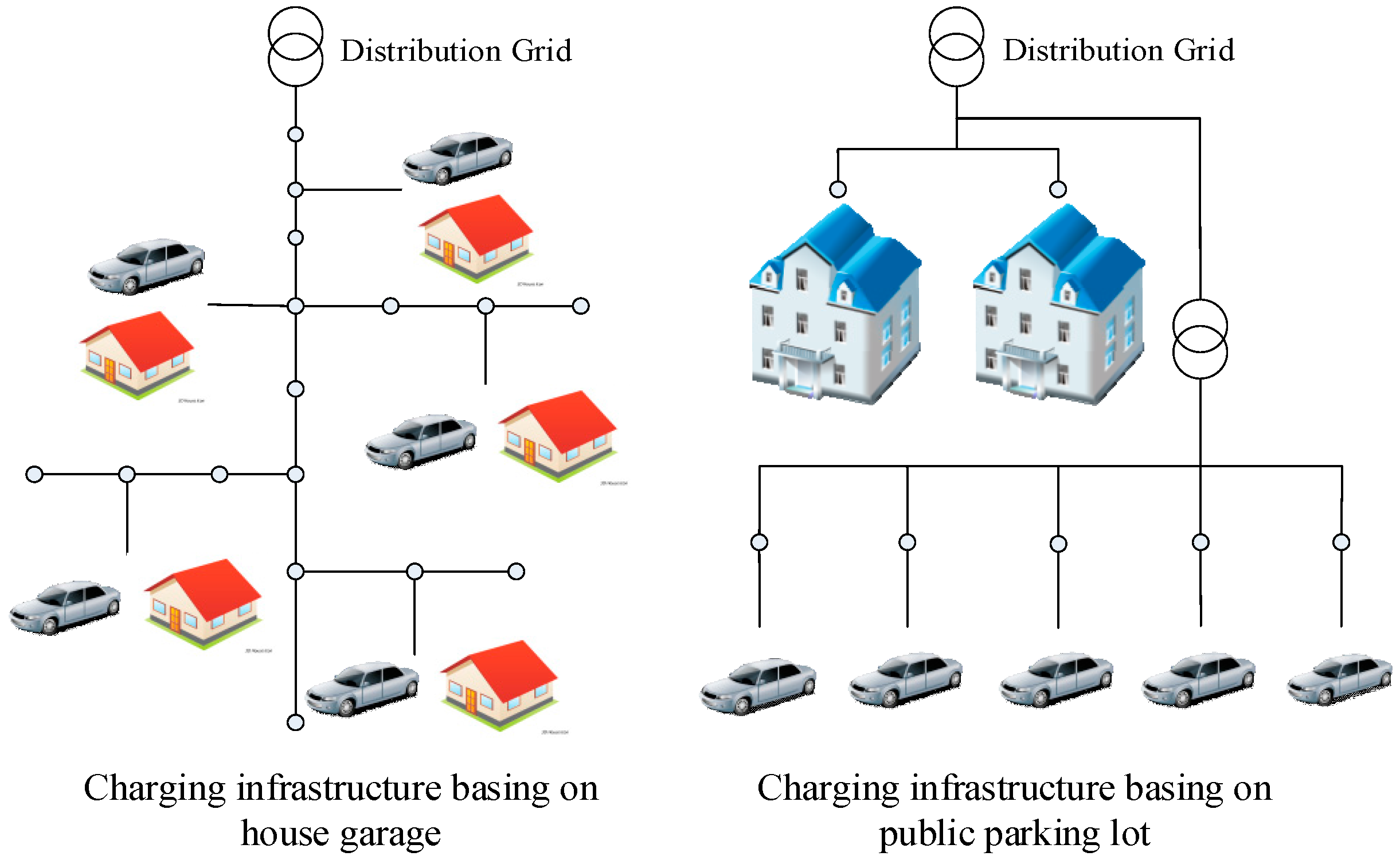
2.1. Regional Distribution Grid Models

EV charging stations can be divided into two typical classes: home-based private garages and dedicated parking lots, shown in Figure 1. EV charging loads in the first class are combined with residential regular loads to affect capacity, voltage profile, and power loss of the existing distribution grids. In highly populated cities, such as major cities in China, the second class is more feasible, due to the lack of private garages and space. In this scenario, a dedicated feeder and transformer must be constructed to support congregated EV charging loads [24]. New feeders are expensive and, hence, it is highly desirable to manage EV charging loads properly to maximize the efficiency and usage of such charging stations.
This paper will focus on EV charging control strategies of the second class. It aims to resolve two issues: (1) smoothen the EV load fluctuations in different charge intervals when the charging stations form a standalone load on a dedicated bus. Addressing this issue will maximize the total number of EVs that can be charged on the station, under a given power rating of the feeder; and (2) minimize the probability of incomplete charging for individual EVs. In other words, all EVs should be fully charged at the end of a predetermined charging period.

2.2. Models of EV Returning-Time and Charging Demand

In this study, we assume that there are M vehicles to be managed on a charging station or a cluster of charging stations on a common feeder. Each vehicle returns home at a random time with a random daily mileage usage, which is translated to the depth of discharge (DOD) of its battery as the charging demand for the evening. The following assumption is common in studies of EV load distribution.
Assumptions:
(1)
The returning time and charging demand of each EV are mutually independent.
(2)
The returning times of all the vehicles are independent and identically distributed (i.i.d.) with density function fs.
(3)
The charging demands of all the vehicles are i.i.d. with density function fD.
The actual statistical information on the returning time and charging demand depends on locations, communities, vehicle types, and many other environmental factors. Studies by the National Household Travel Survey (NHTS) in 2001 [25,26] have reported some typical statistical models, which will be used in this paper for simulation. The returning time of EVs obeys a truncated (to a 24-hour period) and piece-wise normal distribution:
f s ( x ) = { 1 σ s 2 π exp [ ( x μ s ) 2 2 σ s 2 ] , ( μ s 12 ) < x 24 1 σ s 2 π exp [ ( x + 24 μ s ) 2 2 σ s 2 ] , 0 < x ( μ s 12 )
where the mean of the returning time is μ s = 17.6   h (5:36 PM) and the corresponding standard deviation is σ s = 3.4   h .
The daily mileage usage Y is log-normal distributed:
f D ( y ) = 1 y σ D 2 π exp [ ( ln y μ D ) 2 2 σ D 2 ] .
If the average vehicle fuel economy is q (kWh/mile), then the charge demand C (kWh) is C = qY, which is also log-normal distributed. For case studies in this paper, energy consumption data of the Nissan Leaf PEV in [27] are used with q = 0.15 kWh/km (0.24 kWh/mile).
Standard EV charging powers vary from country to country. For example, in the US, the on-board charger power levels are 1.4 kW, 2kW, 6 kW, etc. [28]. In Europe, the most common on-board charger power levels are 3.6 kW and 7.2 kW [29]. In this paper the Chinese standard is used, which specifies the maximum output power of on-board chargers p max = 3.3 kW with rated voltage of 220 V and current of 16 A [30].
To reduce costs, in this paper, the EVs are to be charged during an off-peak low-price period. For example, a typical off-peak electricity price period in Beijing is from 11 PM to 7 AM [31]. Since the charging starting time (11 PM) is far from the expectation of the EV returning time (5:36 PM), and most EVs (greater than 90%) have returned home by 11 PM, according to the probability distribution of returning time of EVs, the probability distribution of returning time of EVs has little impact on the total charging demand of all the EVs.

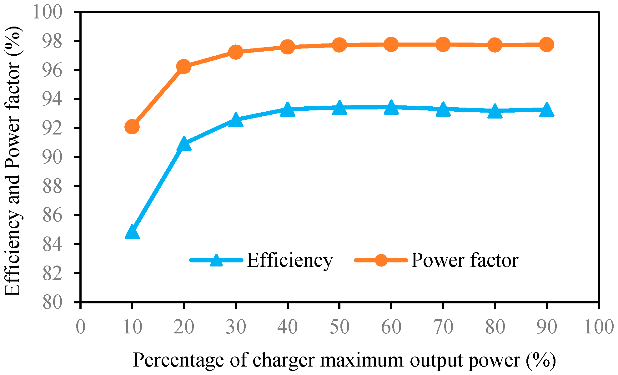
2.3. Efficiency Analysis of On-Board Chargers

A feature of high-frequency power electronics is that its conversion efficiency deteriorates significantly under lower power operation, due to increased switching loss [32]. Figure 2 is a representative efficiency chart, indicating a sharp drop of charger efficiency when the operating power falls below 30% of the rated power. Figure 2 also indicates that the power factor (real power/apparent power) drops, adversely affecting grid voltage control and VAR compensation.
Most of existing load control strategies manage EV loads by regulating charging power continuously without considering charger efficiency and power factor impact. Let the predetermined off-peak period be [ t start , t end ] of duration T = t end t start (hours). The percentage of vehicles that are charged below 30%. p max can be obtained from Equation (2) as P { Y 0.3 p max T / q } = 0 0.3 p max T / q f D ( y ) d y , which increases with augmented T.
To quantitatively examine this issue, we and the China Automotive Engineering Research Institute tested the efficiency and power factor of the charger on an E150, which is produced by Baic Motor Corporation, and the rated power of the on-board charger is 3.3 kW. Under a different charge duration T, the constant charging power of each EV can be obtained. Then we can see percentages of EVs with the charging power lower than 0.3 pmax, and the average efficiency can also be calculated. Table 2 lists the loss of power efficiency under the constant power strategy.
From Table 2, we can see that the longer the charge duration T is, the lower the constant average charging power. That means more EVs have charging power lower than 0.3 pmax, and we will lose more power efficiency. To achieve high charger efficiency under a fixed T, we introduce a random switching control mechanism. In this strategy, the charging period is divided into small segments. The control strategy determines whether to turn on or turn off the charger with a constant power within the high-efficiency range. The charging power control is realized by controlling the percentage of “turn-on” segments. This will be detailed in the next section.
This control mechanism entails on-off-type charging profiles of constant current to the battery system. Since capacity degradation of Li-ion batteries is mainly affected by operational temperature, charge-discharge rate, DOD, among other factors [33,34], within normal charging current and temperature ranges, the constant current profiles are desirable for reducing battery aging effects [35]. In addition, the intermittent charging process is beneficial to the completion of the Li-ion diffusion reaction and can reduce the possibility of Li-ion deposits at the anode [36,37]. It is also noted that since the decision interval for charging current control is typically 5–15 min (300–900 s), the current switching frequency is extremely low (0.0011–0.0033 Hz). Consequently, our strategy will not have a negative impact on normal battery operation or aging.

3. Autonomous Stochastic Charging Control Strategy (ASCCS)

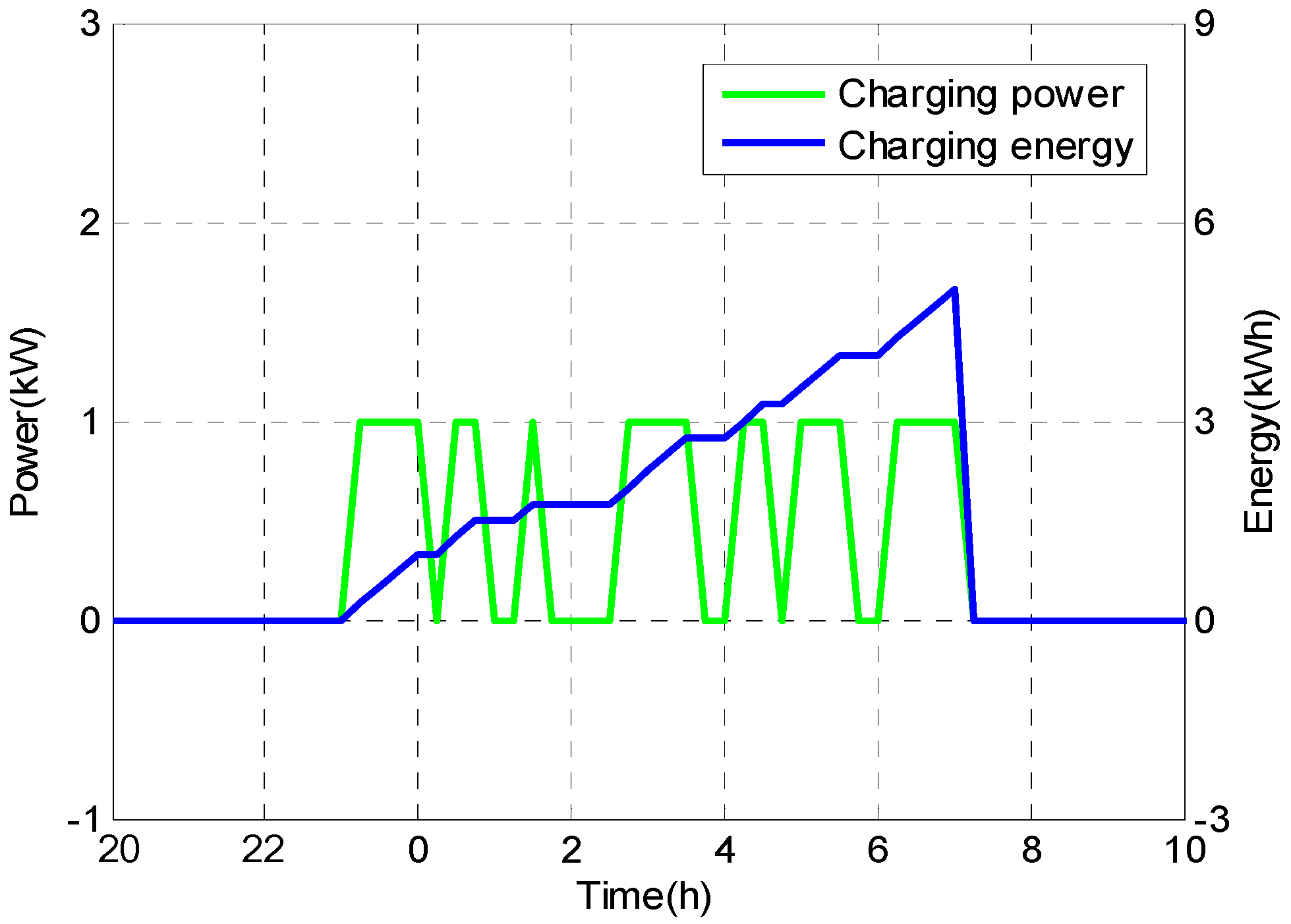
3.1. Basic Control Strategy

The charging period [ t start , t end ] of duration T = t end t start is divided into N time blocks of Δ T = 60 T / N (minutes) each, indexed by k = 1 , , N . Suppose that the constant charging power is p c . Then, the ith vehicle’s charge demand C i , which is i.i.d. and log-normal distributed with density function ln N ( μ C , σ C 2 ) and the nth moment m n = E ( C i n ) = e n μ C + n 2 σ C 2 / 2 , is converted into the required number X i of the time blocks X i = 60 C i / p c Δ T = C i N / p c T . Let C = [ C 1 , , C M ] .
We aim to reduce power variations among time blocks and among different days. We introduce a randomized autonomous control strategy in which each EV does not receive any information about the fleet. Suppose that u i ( k ) , i = 1 , , M , k = 1 , , N are i.i.d. in i and k, and uniformly distributed u i ( k ) U [ 0 , 1 ] . The charging power control for the ith vehicle in the kth block is
λ i ( k ) = p c I { u i ( k ) C i p c T }
where I A is the indicator function: I A = 1 if A is satisfied; I A = 0 , otherwise. As a result, the conditional expectation of λ i ( k ) is E [ λ i ( k ) | C i ] = C i / T . The total charge power of the kth block is p E V ( k ) = i = 1 M λ i ( k ) . Apparently, p E V ( k ) is i.i.d. in k, and its conditional expectation and variance can be calculated [38] as
μ ( C ) = E [ p E V ( k ) | C ] = i = 1 M E [ λ i ( k ) | C i ] = i = 1 M C i / T
V ( C ) = E [ ( p E V ( k ) μ ( C ) ) 2 | C ] = p c T i = 1 M C i ( 1 C i p c T ) .
On the other hand, for each vehicle, the total charge over the entire period is ρ i ( N ) = T N k = 1 N λ i ( k ) . The goal is to complete the required charge C i at t end . The probability of either undercharge or overcharge by a tolerance ε > 0 is P { | ρ i ( N ) C i | > ε } , which is a measure of charge completion.
Charging control aims to achieve the following goals: (a) reduce power fluctuations over the time blocks, namely to reduce V(C); and (b) reduce P { | ρ i ( N ) C i | > ε } . Since both V(C) and P { | ρ i ( N ) C i | > ε } are random variables, their statistical properties will be analyzed in the next subsections.

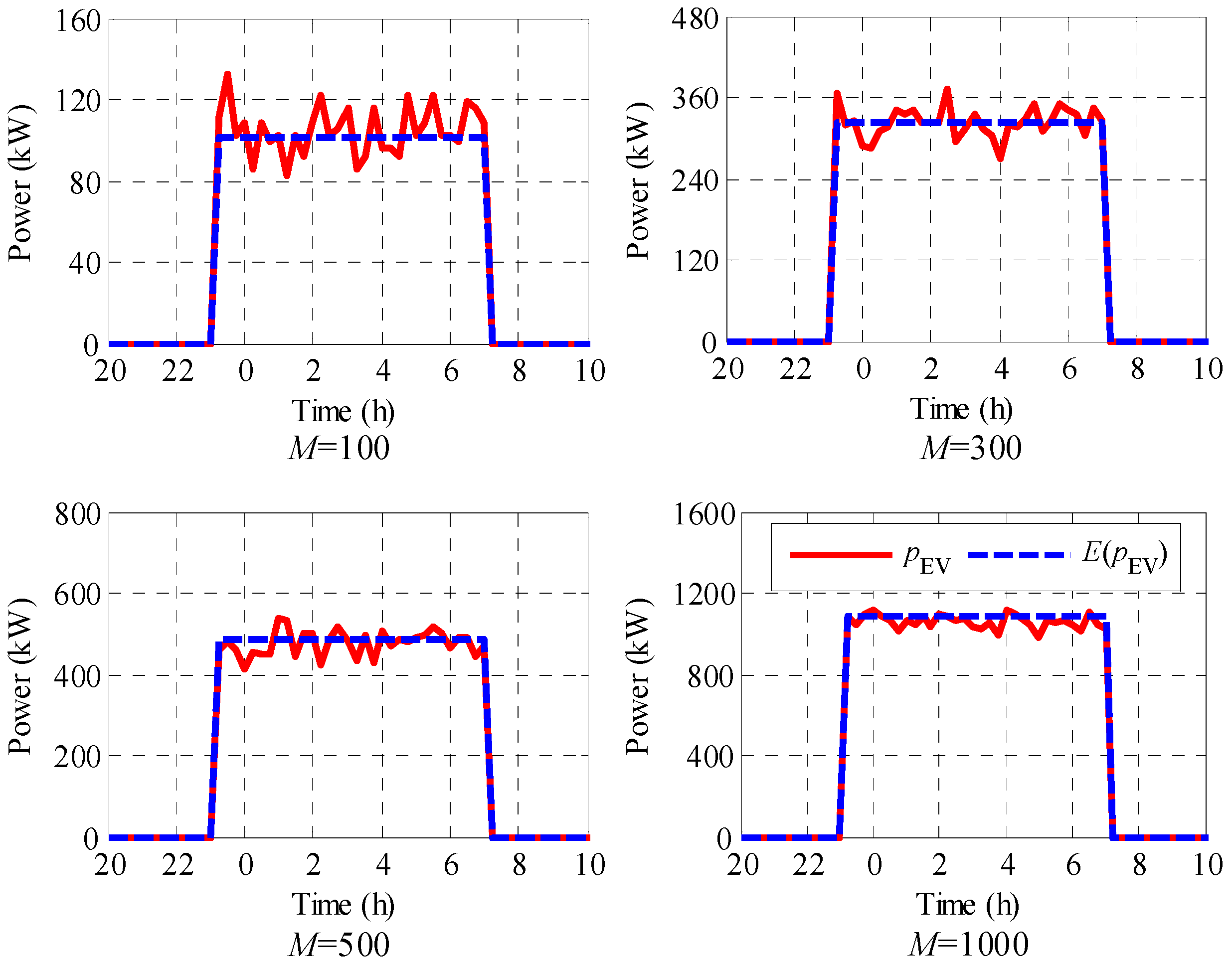
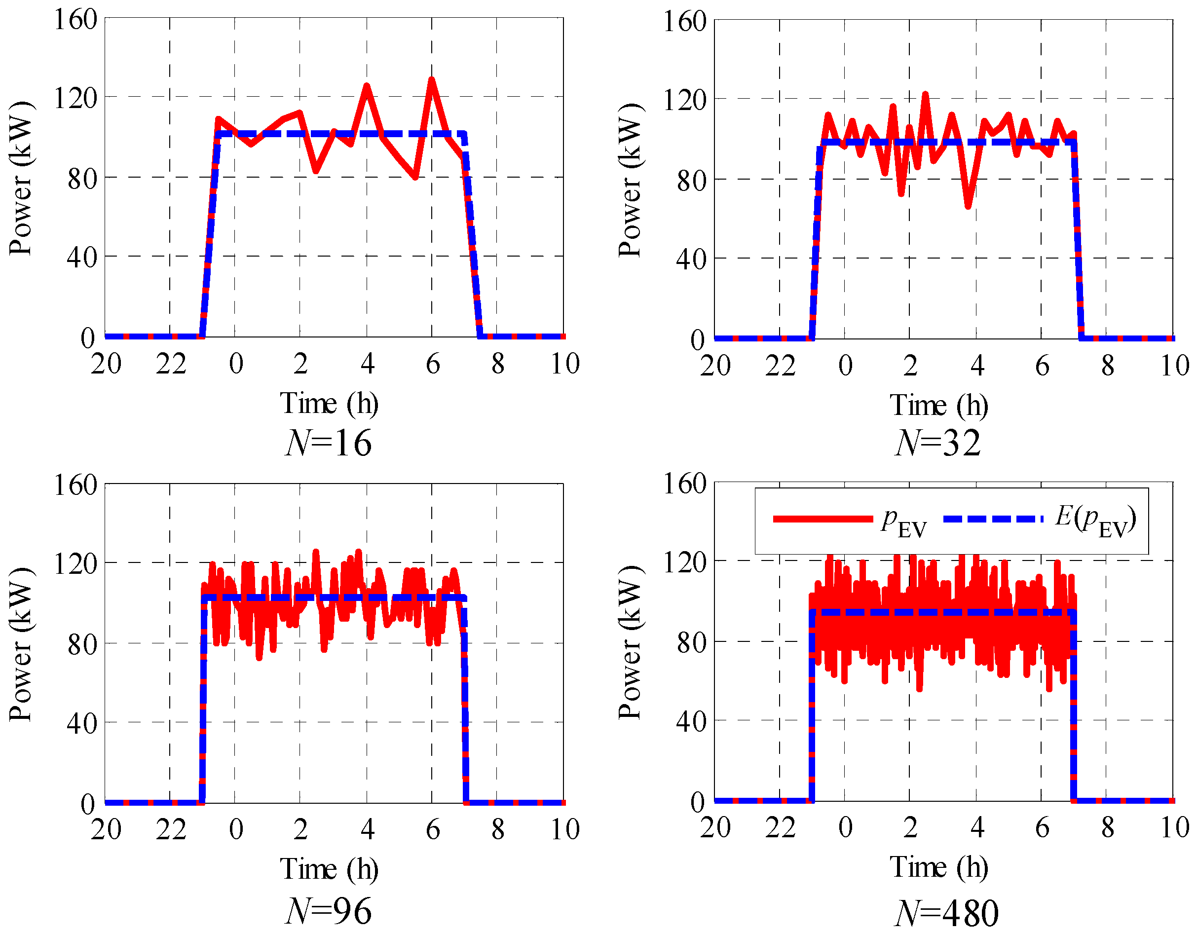
3.2. Power Variation Analysis

To be scalable for charging stations of different sizes, we consider the relative power variations by the average fleet power demand:
η ( C ) = V ( C ) m 1 M = p c m 1 M T i = 1 M C i ( 1 C i p c T ) .
Now, the expectation and variance of η ( C ) can be derived as
η = E [ η ( C ) ] = p c m 1 M T i = 1 M E [ C i ( 1 C i p c T ) ] = p c m 1 M T i = 1 M ( E ( C i ) E ( C i 2 ) p c T ) = p c m 1 T ( m 1 m 2 p c T )
v = E ( ( η ( C ) η ) 2 ) = ( p c m 1 T ) 2 1 M 2 i = 1 M ( m 2 2 m 3 p c T + m 4 ( p c T ) 2 ( m 1 m 2 p c T ) 2 ) = 1 M ( p c m 1 T ) 2 ( m 2 2 m 3 p c T + m 4 ( p c T ) 2 ( m 1 m 2 p c T ) 2 ) = τ M .
Theorem 1.
Under Assumption 1, the following convergence properties hold:
( a )   η ( C ) η , M , w i t h   p r o b a b i l i t y   1 ( w . p . 1 ) . ( b )   η ( C ) η , M ,   in   the   mean   sense ( c )   M ( η ( C ) η τ ) N ( 0 , 1 ) , M ,   in   distribution .
Proof of Theorem 1.
(a)
Let z i = C i ( 1 C i p c T ) . By Assumption 1, z i is i.i.d. Since η ( C ) = p c m 1 T M i = 1 M z i , by the strong law of large numbers, η ( C ) p c m 1 T E [ z i ] = η ,   w . p . 1 .
(b)
This follows directly from lim M v = 0 .
(c)
This is the Central Limit Theorem [38,39]. ☐
Remark 1.
Theorem 1 shows that for a large fleet, the variance of power fluctuations over different time blocks approaches η , which is independent of the size N of the time blocks. In this sense, this is an irreducible power variation. η can be reduced if p c is decreased or T is increased. This fact will be used to improve power variations subsequently. Further reduction of power variations will be pursued by using battery storage devices.
Under the log-normal distribution of Equation (2) with μ D = 3.2 , σ D = 0.88 (daily mileage average e μ D + σ D 2 / 2 = 36.12 miles), and the rated power p max = 3.3 kW , variations of p E V ( k ) and the desired average charging power of all vehicles in the charging duration E ( p E V ) under different M are shown in Figure 3, and its statistics are listed in Table 3.
The simulation results show that power fluctuations are smaller for larger EV fleets, which is consistent with the result of Equation (8). However, in practice, the number of EVs within a regional distribution grid is constrained by its power capacity, the parking space, among others, and usually the power capacity is sufficient in the regional distribution grid with a small number of EVs. Algorithm improvements for relatively small fleets will be presented in the Section 4.

3.3. Charge Completion Analysis

Consider now the total charge for the ith vehicle ρ i ( N ) = T N k = 1 N λ i ( k ) , whose conditional expectation is E [ ρ i ( N ) | C i ] = T N k = 1 N E [ λ i ( k ) ] = C i and conditional variance V a r [ ρ i ( N ) | C i ] = C i ( T p c C i ) / N . The following theorem establishes convergence properties.
Theorem 2.
Under Assumption 1 and the control strategy given by Equation (3), given C i ,
( a )   ρ i ( N ) C i , N , w . p . 1 . ( b )   ρ i ( N ) C i , N ,   in   MS ( c )   N ρ i ( N ) C i C i ( T p c C i ) N ( 0 , 1 ) , N ,   in   distribution
Proof of Theorem 2.
Since the variables λ i ( k ) are i.i.d., it is well known that it is a strong ergodic sequence [38,39,40]. Consequently, its sample means converge to its expectation, in both MS sense and w.p.1. These establish Claims (a) and (b). Claim (c) is the central limit theorem (pp. 278–284, [39]) for i.i.d. sequences. ☐
Given a (small) energy tolerance ε of either earlier completion ρ i ( N ) C i + ε or later completion ρ i ( N ) C i ε , by Chebyshev’s inequality (p. 151, [39]),
P { | ρ i ( N ) C i | ε } C i ( p c T C i ) ε 2 N = α .
If the probability confidence level α = 0.05   or   α = 0.01 , the corresponding energy tolerance is
ε = C i ( p c T C i ) α 1 N .
Put another way, for large values of N, the energy deviation from charge completion vanishes at the rate 1 / N .
We now establish the optimality of the control strategy of Equation (3). In fact, we will show that in a very concrete sense, Equation (3) is the only acceptable strategy.
For any given constant 0 < b < 1 , let a control strategy be defined as λ ˜ i ( k ) = p c I { u i ( k ) b } . Then, ρ ˜ i ( N ) = T N k = 1 N λ ˜ i ( k ) .
Theorem 3.
If b C i p c T , then there exists ε > 0 such that lim N P { | ρ ˜ i ( N ) C i | ε } = 1 .
Proof of Theorem 3.
Suppose b > C i / p c T . Select ε = 1 2 ( p c T b C i ) . Then C i + ε = p c T b ε . From E [ ρ ˜ i ( N ) ] = T N k = 1 N E [ λ ˜ i ( k ) ] = p c T b , by Chebyshev’s inequality,
lim N P { ρ ˜ i ( N ) C i + ε } = 1 lim N P { ρ ˜ i ( N ) p c T b ε } = 1 .
Similarly, if b < C i / p c T , we have lim N P { ρ ˜ i ( N ) C i ε } = 1 . ☐
Remark 2.
Theorem 3 claims that if another control strategy, different from Equation (3), is used, then for large values of N, with near certainty, it will lead to either premature or late charge completion. In this sense, the control in Equation (3) is optimal.
Under M = 100, charging power with different numbers of time blocks are depicted in Figure 4, whose power fluctuations are roughly equal to Theorem 1. The statistics on charge completion with different values of N are listed in Table 4.
Table 4 concludes that the smaller the time block is, the less likely the charge will be complete. This conclusion is consistent with the previous theoretical analysis. Since the number of time blocks is restricted by the minimum switching cycle of on-board chargers due to switching loss, we will introduce improvement policies for relatively small values of N.

4. Implementation and Improvements of ASCCS

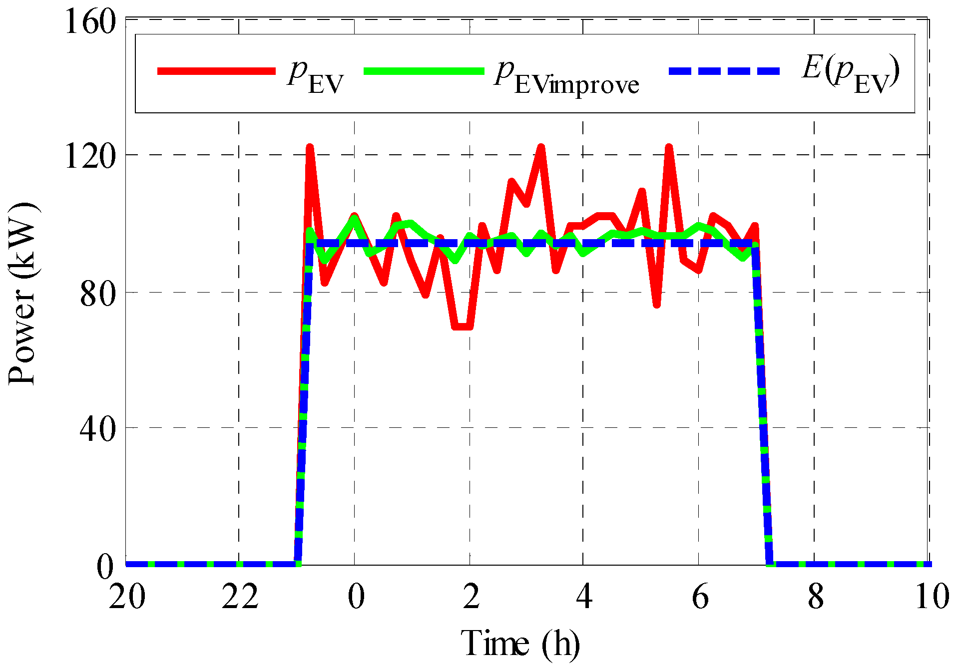
4.1. Individualized Power Management for Reducing Power Variations

From Equations (6) and (7), the daily and average variances of power fluctuations are proportional to the charging power p c . To reduce power fluctuations among time blocks, it is favorable to have large T and small p c . However, in our control strategy, we do not try to change T, and we just want to obtain an optimal pc to ensure both charging efficiency and power fluctuations under the constraint that the EVs are fully charged. From Figure 2, as long as the charge power is above 0.3 p max , charging efficiency remains high.
Based on this observation, we introduce the following power reduction algorithm: for the ith EV, we first calculate the average charging power p = C i / T . Then the actual charging power is max { p , 0.3 p max } . Figure 2 confirms that the efficiency is above 92.5% when the charging power is above 0.3 p max . Additionally, by using lower power, power fluctuations are reduced. Figure 5 compares power fluctuations with and without applying the power reduction algorithm and verifies that this algorithm is able to reduce substantially the power variations.

4.2. Adaptive Charging Control for Improving Charge Completion

The control strategy of Equation (3) is i.i.d. and non-adaptive. As shown in Table 4, for small values of N, charging completion is unsatisfactory. For N = 32, 11.2% EVs will suffer from an incomplete charge. To ensure charge completion, we introduce an adaptive charging control that adapts its charging probability at each k, based on the remaining charging demand.
Let the required number of blocks for charging completion be X i = C i N p c T . Then, the control (Equation (3)) is modified to
λ i ( k ) = p c I { u i ( k ) f i ( k ) }
where f i ( k ) = ( X i c i , k 1 ) / ( N k ) , k = 1 , 2 , ...... , N , and c i , k 1 = j = 1 k 1 I { u i ( j ) f i ( j ) } is the actual number of the charging blocks up to k – 1. The strategy (Equation (11)) is based on the following ideas:
(a)
If at any k = k 0 1 < N , c i , k 1 = X 0 , namely, the EV is fully charged, then f i ( k ) = 0 , k = k 0 , ...... , N . Hence, overcharging is avoided.
(b)
If at any k = k 0 1 < N , X i c i , k 0 1 = N k 0 , namely, the remaining charging demand is equal to the remaining available blocks, then f i ( k ) = 1 , k = k 0 , ...... , N . Hence, incomplete charging is avoided.
(c)
Otherwise, this strategy ensures that E λ i ( k ) = p c X i c i , k N k is the optimal average power for completing the charge over the remaining blocks based on Theorem 3. Indeed, if we view the remaining charge demand at k as C ˜ i ( k ) = p c ( X i c i , k ) Δ T and the remaining time as T ˜ ( k ) = ( N k ) Δ T , then f i ( k ) = C ˜ i ( k ) p c T ˜ ( k ) i , which is consistent with the optimal strategy in Theorem 3.
Due to these features, this adaptive strategy will guarantee that all EVs will be fully charged at the end without overcharging. This is stated in the following theorem with its proof included in the Appendix.
Theorem 4.
For any 1 i M , c i , N = X i , with possibility 1 (w.p.1).
Proof of Theorem 4.
Show that c i , N = X i for any 1 i M , if the ith EV charging probability in the kth time block is determined by
f i ( k ) = X i c i , k 1 N ( k 1 ) , k = 1 , 2 , ...... , N .
We prove this theorem by contradiction, namely, it is impossible to have c i , N > X i or c i , N < X i .
The charging probability is determined by the following recursive formulas:
{ p ( c i , k = c i , k 1 ) = 1 ( X i c i , k 1 ) / ( N ( k 1 ) ) p ( c i , k = c i , k 1 + 1 ) = ( X i c i , k 1 ) / ( N ( k 1 ) ) .
(1)
Assume that c i , N > X i . Noticing that c i , k is monotonically increasing over k and c i , 0 = 0 , it follows that there must exist c i , l = X i for some 1 l N 1 by the assumption c i , N > X i . However, we have
p ( c i , l + 1 = c i , l + 1 ) = ( X i c i , l ) / ( N ( N l ) ) = 0
which derives that c i , j = X i for any l j N . This contradicts the assumption c i , N > X i .
(2)
Assume c i , N < X i . Thus, we have c i , N 1 X i 1 . In the case that c i , N 1 = X i 1 , we have
p ( c i , N = c i , N 1 + 1 ) = ( X i c i , N 1 ) / ( N ( N 1 ) ) = 1 .
Namely c i , N = X i , which contradicts the assumption c i , N < X i . It can be shown that
0 p ( c i , k = c i , k 1 + 1 ) = ( X i c i , k 1 ) / ( N ( k 1 ) ) 1
by the charging probability formulas given before. In the case that c i , N 1 < X i 1 , we have
p ( c i , N = c i , N 1 + 1 ) = ( X i c i , N 1 ) / ( N ( N 1 ) ) = X i c i , N 1 > 1
which contradicts 0 p ( c i , N = c i , N 1 + 1 ) 1 . Therefore, we prove that c i , N = X i . ☐

4.3. Simulation on Improved ASCCS

Considering a typical residential community in Beijing with 400 families and 100 EVs (25% penetration), namely M = 100, and the rated power p max = 3.3 kW . Under the same log-normal daily mileage distribution, and N = 32, charging power curves using the original and adaptive ASCCS are shown in Figure 5. The charging power and charging energy curves of one EV, which has the charging demand of 4.9 kWh are demonstrated in Figure 6.
From the simulation results, the power fluctuations of the EV charging power are reduced from 29% to 6%, and all of the EVs are fully charged within the predetermined charging period using the adaptive approach.
It is noted that even for a large M, the variance η = p c m 1 T ( m 1 m 2 p c T ) in Equation (7) has an irreducible value. To further reduce power fluctuations, a battery system [41] may be leveraged to absorb instantaneous power variations between blocks. In Section 5, we introduce battery systems to support grid-level load smoothing.

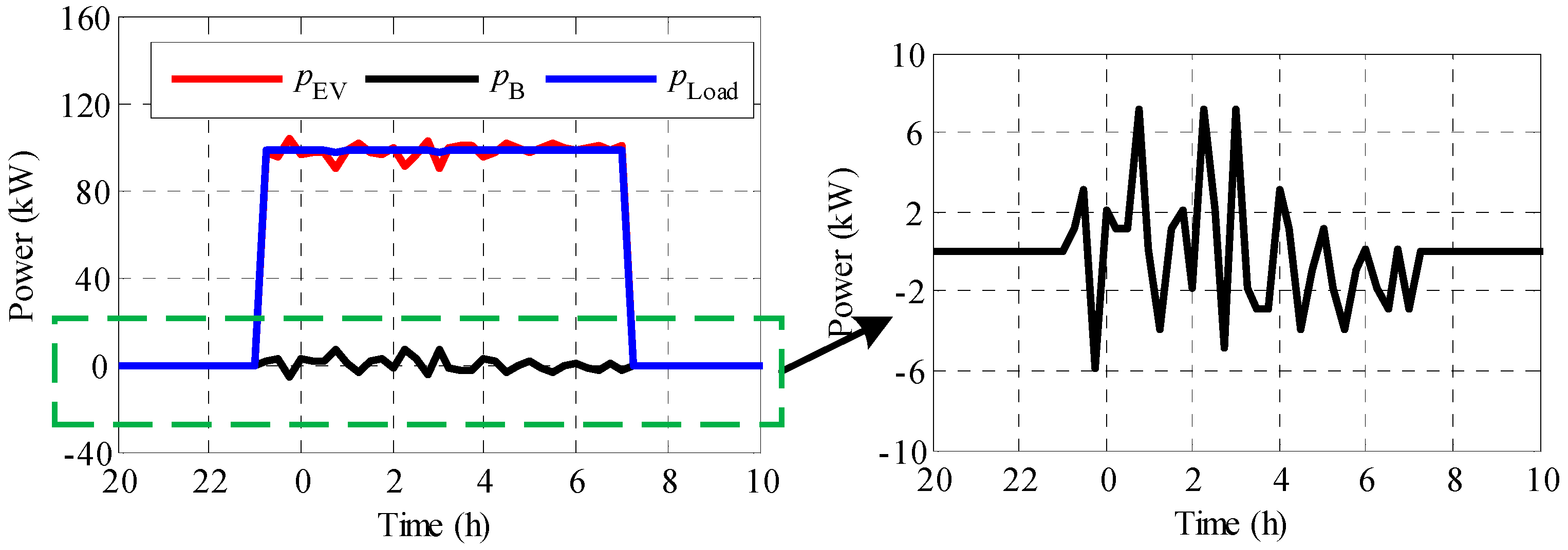
5. Grid-Support Battery Storage for Reducing Power Variations

5.1. Analysis

From Equation (4), μ ( C ) = E [ p E V ( k ) | C ] = i = 1 M C i / T . The battery system is controlled as follows: if p E V ( k ) is below μ ( C ) , the battery system is discharged to inject power to the grid; and if p E V ( k ) is above μ ( C ) , the battery system is charged to receive power from the grid. Intuitively, the larger the energy capacity (kWh) is, the smoother the EV load p E V ( k ) becomes.
To understand this intuition more rigorously, we assume that the battery system has the maximum power rating p b max for both charge and discharge operations, and the battery energy capacity is Q (kWh). Consequently, the battery power output is:
p B ( k ) = min { p b max , | p E V ( k ) μ ( C ) | } × sign ( p E V ( k ) μ ( C ) )
where p B ( k ) > 0 is charged and p B ( k ) < 0 is discharged. Consequently, the battery-supported load power becomes:
p L o a d ( k ) = p E V p B ( k )
It is easy to verify that E [ p B ( k ) | C ] = 0 , hence the compensation is unbiased and E [ p L o a d ( k ) | C ] = μ ( C ) . However, the variance of p L o a d ( k ) is much smaller than p E V ( k ) . This is apparent from:
p L o a d ( k ) = { 0 ,   if   | p E V ( k ) μ ( C ) | p b max p E V ( k ) p b max ,   if   p E V ( k ) μ ( C ) > p b max p E V ( k ) + p b max ,   if   p E V ( k ) μ ( C ) < p b max
The battery system’s SOC S ( k ) is also a random process:
S ( k ) = S ( 0 ) + Δ T Q j = 1 k p B ( k )
Since p B ( k ) is an i.i.d. process of zero mean, S ( k ) is a stationary process with an independent increment and, in particular, a martingale. The battery system has its SOC bounds S min S ( k ) S max . When S ( k ) = S max , its charge operation is disabled, and when S ( k ) = S min , its discharge operation is disabled. As a result, S ( k ) is a bounded (or truncated) stochastic process, see [38,40] for its convergence properties and error analysis. We now use a case study to demonstrate the effectiveness of battery assistance in alleviating power fluctuations and dependence of such effectiveness upon p b max and its energy capacity.

5.2. A Case Study

Let us consider the same scenario in Section 4, but add a grid-support battery storage system. Assume that 30 % S ( k ) 100 % . The simulation results are summarized in Table 5.
In Table 5, we have set three scenarios in which the maximum power fluctuations are reduced to 5%, 3%, and 1%, accordingly, to compare with the case without a battery, then do the simulation and try to obtain the energy capacity to meet the demand. From the simulation results, we can see that with support from the battery storage system with relatively small energy capacity, the power fluctuations are noticeably curtailed. For example, with a battery system with a maximum power of 7 kW and an energy capacity of 14 kWh, the charge station of 100 EVs with a total load of 785 kWh has its maximum power fluctuations below 1%. However, this battery storage system is optional since the power fluctuation is as low as 6% without a battery storage system, and it can be applied in some special scenarios. The simulation results of Case 4 are presented in Figure 7, where pEV is the EV charging load curve without the battery energy storage system, pload is the EV charging load curve after using the battery energy storage system, and pB is the power output curve of the battery energy storage system.
It can be seen that the EV charging power curve is smoothened after adding a battery storage system of very small capacity. It will cost little since the battery capacity is very small. One interpretation is that by using a randomized control strategy, the probability of consecutive high (or low) power time blocks are very small. This implies that the battery experiences frequent charge/discharge alternations and its SOC remains in the middle range with very high probability. Consequently, a seemingly small battery system can achieve substantial reduction on power fluctuations. This feature is highly appealing for applications due to its economic benefits.

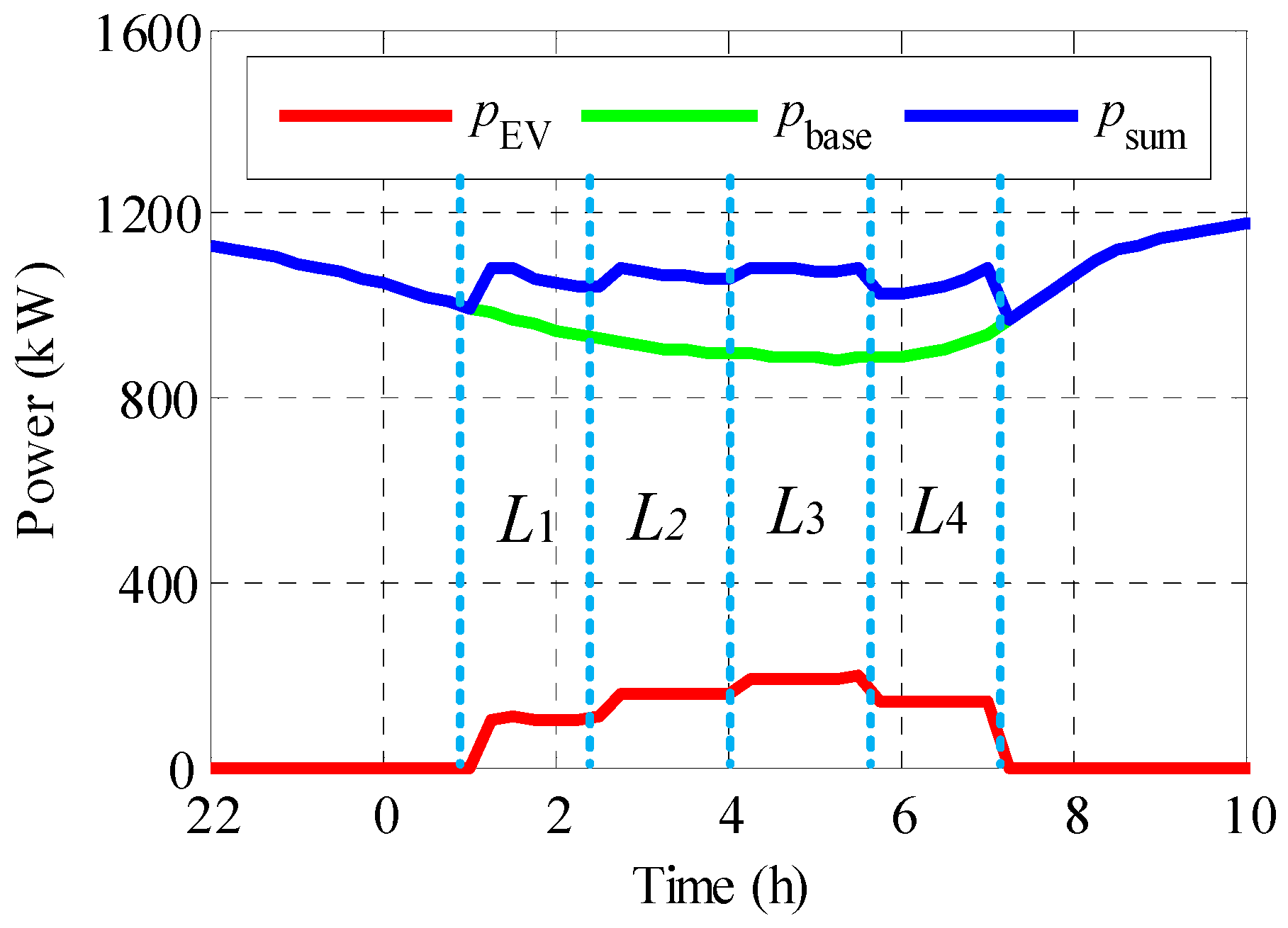
6. Application of the ASCCS Method in Valley-Filling Problems with a Conventional Load

If a regional distribution grid is loaded with both EV charging demands and regular loads, it is possible that the EV loads can be managed to fill load valleys. Consider the problem of managing EV loads such that: (a) EV loads are placed during an interval of low regular loads; and (b) during this interval, the combined regular and EV loads are smoothened over designated time blocks. The regular load p b a s e ( k ) is time-varying. Assume that p b a s e ( k ) has been obtained by historical data analysis and known in EV load management. This assumption is valid for the experimental site of this study where daily variations of p b a s e ( k ) are very small.
To approach this problem, we employ a two-time-scale methodology. The main idea of our control strategy can be summarized as follows:
(a)
Based on the information on the regular loads p b a s e ( k ) and daily EV load demand C, the grid scheduler assigns a time interval [ T 1 , T 2 ] [ t s t a r t , t s t a r t + T ] to be the interval of the valley-filling operation.
(b)
[ T 1 , T 2 ] is divided into N time blocks, which are then grouped into L phases of K = N / L blocks each (for simplicity, let K be an integer). The new charging duration in each phase is
T = ( T 2 T 1 ) / L .
(c)
For the ith EV, its daily charge demand C i is distributed to each phase as C i ( l ) such that l = 1 L C i ( l ) = C i .
(d)
Within each phase, the adaptive ASCCS algorithm, described in Section 4.2, is applied, which reduces load fluctuations among the time blocks in each phase and guarantees that the charge demand C i ( l ) will be completed at the end of each phase.
The control goal is to keep the sum of the EV loads and conventional loads as flat as possible during the charging period. We now detail these steps.
First, we should determine the “valley-filling” target, namely, the expected sum of the EV charging load and conventional load. Thus, we can calculate the expected EV load in different phases with respect to the conventional load data and the “valley-filling” target. Suppose that a constant b satisfies the following conditions:
{ b = p b a s e ( T 1 ) = p b a s e ( T 2 ) ( T 2 T 1 ) b = k = 1 N p b a s e ( k ) + i = 1 M C i .
It follows that the expected charging load in the lth phase is
max { 0 , b T p b a s e ( l ) }
where p b a s e ( l ) is the total conventional loads in the lth phase.
The charge demand of the ith EV in the lth phase is
C i ( l ) = b T p b a s e ( l ) l = 1 L ( b T p b a s e ( l ) ) × C i .
Finally, the adaptive ASCCS (Equation (11)) is employed with T, replaced by T from Equation (16) and C i by C i ( l ) from Equation (19).
At the starting time of the valley-filling operation, the charging service provider transmits the information on the expected regular loads to each EV. The “valley-filling” control utilizes such information to implement the adaptive ASCCS. There is neither bi-directional data transmission between the EVs and the central control system nor the real-time global control signal during the charging period.
Consider the same simulation conditions as in Section 4, but add conventional loads from the residential users. Divide the “valley-filling” period into four phases, L1, L2, L3, and L4. In each phase, the total charge load variations from the adaptive ASCCS and the total load trajectories are demonstrated in Figure 8, where pEV is the EV charging load by using the proposed improved ASCCS, pbase is the conventional load, and psum is the sum of the EV charging and conventional loads. It is evident that in each phase the EV charging loads are close to their average. Hence, the goal of “valley-filling” for the whole charging period is approximately fulfilled. It also reveals that more phases and more blocks will result in to more effective “valley-filling”.

7. Conclusions

The ASCCS proposed in this paper is essentially a strategy that uses uniform random numbers created by the EVs themselves to control the charging probability for achieving the average charging load within the charging period. The charging strategy proposed in the paper can always make the on-board charger work in the high efficiency operational range, does not need the central processing unit to provide a common reference signal, and it really fulfills the unidirectional data transmission of the whole control system. Further improvements on the core strategy, including individualized power management, adaptive strategies, and battery support systems, are introduced to reduce power variances and to guarantee charge completion. These desirable properties are established by rigorous analysis and verified by simulations and case studies. A battery energy storage system with small capacity is employed to further reduce the charging load fluctuation, and effective “valley-filling” also can achieve by using the proposed strategy.
While this paper concentrates on EV load management, the key principles are readily extendable to charging infrastructures powered by intermittent renewable energy sources, e.g., solar and wind power. For instance, by employing power-generating characteristics of photovoltaic (PV) systems and/or wind generators, EV charging probabilities are adapted to procure maximum energy utilization and to power demand perturbations to regional distribution grids.
There are some important open issues along the direction of this paper. In this work, off-line forecasting of regular loads is used in the valley-filling operation. In consideration of load changes due to holidays, events, and weather conditions, more precise control schemes can potentially be developed by means of more advanced predictive control algorithms.

Acknowledgments

This work was supported by the National Key Technology Support Program (Grant Number 2013BAA01B03).

Author Contributions

Weige Zhang proposed the research topic and designed the model. Di Zhang programmed the algorithms. Le Yi Wang performed theoretical analysis and proof. Di Zhang and Le Yi Wang organized the paper. Biqiang Mu performed calculations. Yan Bao and Jiuchun Jiang took part in validating the idea and revising the paper. Hugo Morais helped to respond to the comments and revise this paper. All authors contributed to the writing of the manuscript, and have read and approved the final manuscript.

Conflicts of Interest

The authors declare no conflict of interest.

References

  1. Liu, Z.; Wu, Q.; Nielsen, A.H.; Wang, Y. Day-ahead energy planning with 100% electric vehicle penetration in the Nordic region by 2050. Energies 2014, 7, 1733–1749. [Google Scholar] [CrossRef] [Green Version]
  2. Alonso, M.; Amaris, H.; Germain, J.G.; Galan, G.M. Optimal charging scheduling of electric vehicles in smart grids by heuristic algorithms. Energies 2014, 7, 2449–2475. [Google Scholar] [CrossRef]
  3. Lindgren, J.; Niemi, R.; Lund, P.D. Effectiveness of smart charging of electric vehicles under power limitations. Int. J. Energy Res. 2014, 38, 404–414. [Google Scholar] [CrossRef]
  4. Liu, J. Electric vehicle charging infrastructure assignment and power grid impacts assessment in Beijing. Energy Policy 2012, 51, 544–557. [Google Scholar] [CrossRef]
  5. Green, R.C.; Wang, L.F.; Alam, M. The impact of plug-in hybrid electric vehicles on distribution networks: A review and outlook. Renew. Sustain. Energy Rev. 2011, 15, 544–553. [Google Scholar] [CrossRef]
  6. Clement-Nyns, K.; Haesen, E.; Driesen, J. The impact of charging plug-in hybrid electric vehicles on a residential distribution grid. IEEE Trans. Power Syst. 2010, 25, 371–380. [Google Scholar] [CrossRef] [Green Version]
  7. Zhang, L.; Brown, T.; Samuelsen, G.S. Fuel reduction and electricity consumption impact of different charging scenarios for plug-in hybrid electric vehicles. J. Power Sources 2011, 196, 6559–6566. [Google Scholar] [CrossRef]
  8. Foley, A.; Tyther, B.; Calnan, P.; Gallachóir, B.Ó. Impacts of electric vehicle charging under electricity market operations. Appl. Energy 2013, 101, 93–102. [Google Scholar] [CrossRef]
  9. Zhang, Q.; Mclellan, B.C.; Tezuka, T.; Ishihara, K.N. A methodology for economic and environmental analysis of electric vehicles with different operational conditions. Energy 2013, 61, 118–127. [Google Scholar] [CrossRef]
  10. Ma, Z.; Callaway, D.S.; Hiskens, I.A. Decentralized charging control of large populations of plug-in electric vehicles. IEEE Trans. Control Syst. Technol. 2013, 21, 67–78. [Google Scholar] [CrossRef]
  11. Soares, J.; Borges, N.; Vale, Z.; Oliveira, P.B.M. Enhanced Multi-Objective Energy Optimization by a Signaling Method. Energies 2016, 9, 807. [Google Scholar] [CrossRef]
  12. Abdelaziz, M.M.A.; Shaaban, M.F.; Farag, H.E.; El-Saadany, E.F. A multistage centralized control scheme for islanded microgrids with PEVs. IEEE Trans. Sustain. Energy 2014, 5, 927–937. [Google Scholar] [CrossRef]
  13. Peng, J.; He, H.; Feng, N. Simulation research on an electric vehicle chassis system based on a collaborative control system. Energies 2014, 61, 312–328. [Google Scholar] [CrossRef]
  14. Antonio, C.; Carlos, P.; David, P.D.; Oscar, M.A. Planning minimum interurban fast charging infrastructure for electric vehicles: Methodology and application to Spain. Energies 2014, 7, 1207–1229. [Google Scholar]
  15. Sortomme, E.; Hindi, M.M.; MacPherson, S.D.J.; Venkata, S.S. Coordinated charging of plug-in hybrid electric vehicles to minimize distribution system losses. IEEE Trans. Smart Grid 2011, 2, 198–205. [Google Scholar] [CrossRef]
  16. Hu, J.; Morais, H.; Sousa, T.; Lin, M. Electric vehicle fleet management in smart grids: A review of services, optimization and control aspects. Renew. Sustain. Energy Rev. 2016, 56, 1207–1226. [Google Scholar] [CrossRef] [Green Version]
  17. Zhang, D.; Jiang, J.; Wang, L.; Zhang, W. Robust and scalable management of power networks in dual-source trolleybus systems: A consensus control framework. IEEE Trans. Intell. Transp. Syst 2016, 17, 1029–1038. [Google Scholar] [CrossRef]
  18. Soares, J.; Ghazvini, M.A.F.; Borges, N.; Vale, Z. A stochastic model for energy resources management considering demand response in smart grids. Electr. Power Syst. Res. 2017, 143, 599–610. [Google Scholar] [CrossRef]
  19. Roy, J.V.; Leemput, V.N.; Geth, F.; Büscher, J.; Driesen, J. Electric vehicle charging in an office building microgrid with distributed energy resources. IEEE Trans. Sustain. Energy 2014, 5, 1389–1396. [Google Scholar]
  20. Zhang, K.; Xu, F.; Ouyang, M.; Wang, H.; Lu, L.; Li, J.; Li, Z. Optimal decentralized valley-filling charging strategy for electric vehicles. Energy Convers. Manag. 2014, 78, 537–550. [Google Scholar] [CrossRef]
  21. Salah, F.; Ilg, J.P.; Flath, C.M.; Basse, H.; Dinther, C. Impact of electric vehicles on distribution substations: A Swiss case study. Appl. Energy 2015, 137, 88–96. [Google Scholar] [CrossRef]
  22. Katarina, K.; Mattia, M. Phase-wise enhanced voltage support from electric vehicles in aDanish low-voltage distribution grid. Electr. Power Syst. Res. 2016, 140, 274–283. [Google Scholar]
  23. Richardson, P.; Flynn, D.; Keane, A. Local versus centralized charging strategies for electric vehicles in low voltage distribution systems. IEEE Trans. Smart Grid 2012, 3, 1020–1028. [Google Scholar] [CrossRef]
  24. Liu, D.; Wang, Y.; Shen, Y. Electric vehicle charging and discharging coordination on distribution network using multi-objective particle swarm optimization and fuzzy decision making. Energies 2016, 9, 1. [Google Scholar] [CrossRef]
  25. Qian, K.; Zhou, C.; Allan, M.; Yuan, Y. Modeling of load demand due to EV battery charging in distribution systems. IEEE Trans. Power Syst. 2011, 26, 802–810. [Google Scholar] [CrossRef]
  26. Tian, L.; Shi, S.; Jia, Z. A statistical model for charging power demand of electric vehicles. Power Syst. Technol. 2010, 34, 126–130. [Google Scholar]
  27. Ashtari, A.; Bibeau, E.; Shahidinejad, S.; Molinski, T. PEV charging profile prediction and analysis based on vehicle usage data. IEEE Trans. Smart Grid 2012, 3, 341–350. [Google Scholar] [CrossRef]
  28. Hadley, S.W.; Tsvetkova, A.A. Potential impacts of plug-in hybrid electric vehicles on regional power generation. Electr. J. 2009, 22, 56–68. [Google Scholar] [CrossRef]
  29. Bakker, S. Standardization of EV Recharging Infrastructures; E-mobility NSR: Delft, The Netherlands, 2013. [Google Scholar]
  30. On-Board Conductive Charger for Electric Vehicles, QC/T 895-2011. Available online: http://www.codeofchina.com/standard/QCT895-2011.html (accessed on 18 January 2017).
  31. Zhang, D.; Jiang, J.; Zhang, W.; Zhang, Y.; Huang, Y. Economic operation of electric vehicle battery swapping station based on genetic algorithms. Power Syst. Technol. 2013, 37, 2101–2107. [Google Scholar]
  32. Jiang, J.; Bao, Y.; Wang, L.Y. Topology of a bidirectional converter for energy interaction between electric vehicles and the grid. Energies 2014, 7, 4858–4894. [Google Scholar] [CrossRef]
  33. Sarasketa-Zabala, E.; Gandiaga, I.; Rodriguez-Martinez, L.M.; Villarreal, I. Cycle ageing analysis of a LiFePO4/graphite cell with dynamic model validations: Towards realistic lifetime predictions. J. Power Sources 2015, 275, 573–587. [Google Scholar] [CrossRef]
  34. Ma, Z.; Jiang, J.; Shi, W.; Zhang, W.; Mi, C.C. Investigation of path dependence in commercial lithium-ion cells for pure electric bus applications: Aging mechanism identification. J. Power Sources 2015, 274, 29–40. [Google Scholar] [CrossRef]
  35. Barré, A.; Deguilhem, B.; Grolleau, S.; Gérard, M.; Suard, F.; Riu, D. A review on lithium-ion battery ageing mechanisms and estimations for automotive applications. J. Power Sources 2013, 241, 680–689. [Google Scholar] [CrossRef]
  36. Monem, M.A.; Trad, K.; Omar, N.; Hegazy, O.; Mantels, B.; Mulder, G.; Van den Bossche, P.; Van Mierlo, J. Lithium-ion batteries: Evaluation study of different charging methodologies based on aging process. Appl. Energy 2015, 152, 143–155. [Google Scholar] [CrossRef]
  37. Li, J.; Murphy, E.; Winnick, J.; Kohl, P.A. The effects of pulse charging on cycling characteristics of commercial lithium-ion batteries. J. Power Sources 2001, 102, 302–309. [Google Scholar] [CrossRef]
  38. Papoulis, A.; Pillai, S.U. Probability, Random Variables, and Stochastic Processes, 4th ed.; McGraw-Hill: New York, NY, USA, 2002. [Google Scholar]
  39. Ash, R.B. Real Analysis and Probability; Academic Press: New York, NY, USA, 1972. [Google Scholar]
  40. Taylor, H.M.; Karlin, S. An Introduction to Stochastic Modeling, 3rd ed.; Academic Press: Chestnut Hill, MA, USA, 1998. [Google Scholar]
  41. Tant, J.; Geth, F.; Six, D.; Tant, P.; Driesen, J. Multiobjective battery storage to improve PV integration in residential distribution grids. IEEE Trans. Sustain. Energy 2013, 4, 182–191. [Google Scholar] [CrossRef]
Figure 1. Comparison of different construction modes of charging infrastructure in a regional distribution grid.
Energies 10 00147 g001
Figure 2. Charger output power vs. efficiency and power factor.
Energies 10 00147 g002
Figure 3. Charging power curves with a different number of electric vehicles (EVs).
Energies 10 00147 g003
Figure 4. Charging power curves with different lengths of time blocks.
Energies 10 00147 g004
Figure 5. Charging power curves using the original and improved autonomous stochastic charging control strategy (ASCCS).
Energies 10 00147 g005
Figure 6. Charging power and charging energy curves of one EV.
Energies 10 00147 g006
Figure 7. Charging power curves with the 14 kWh battery storage system.
Energies 10 00147 g007
Figure 8. Load curves of the regional distribution grid considering a conventional load.
Energies 10 00147 g008
Table 1. List of key symbols.
SymbolExplanation
MNumber of EVs
CiAverage daily charging demand of the ith EV
pmaxMaximum output power of on-board charger
pcEV charging power
TEV charging time period
tstartEV charging start time
tendEV charging end time
λ i ( k ) The charging power for the ith vehicle in the kth time block
Δ T Length of one time block
NNumber of time blocks
ρ i ( N ) The total charging energy of ith EV in the entire time period
fi(k)The ith EV charging probability constant in the kth time block
XiNeeded number of time blocks for the ith EV
c i , k 1 Number of time blocks charged for the ith EV after k − 1 time blocks
pEV(k)The EV charging power in the kth time block
pB(k)The battery output in the kth time block
PLoad(k)The battery-supported load power in the kth time block
S(k)SOC (State of Charge) of the battery storage system in the kth time block
QThe energy capacity of the battery storage system in the kth time block
pbase(k)Regular load of regional distribution gird
LNumber of the phases that the whole charging period is divided into considering the regular load
T’The new charging duration in each phase
BDesired value of sum of regular load and EV charging power in the regional distribution gird
Ci(l)The charging demand of the ith EV in lth phase
Table 2. Charging power efficiency with different T.
Charge Duration T (Hour)6789
%   o f   EVs   with   p c < 0.3 p max 69.2%81.3%89.0%93.5%
Average efficiency91.3%90.4%89.5%88.7%
Table 3. Power fluctuations of charging power for different number of EVs.
Number M of EVs1003005001000
Maximum power fluctuation29%15%12%6%
Table 4. Charge completion statistics with different values of N.
Number N of Time Blocks163296480
Charge completion86.6%88.8%94.5%97.2%
Table 5. Power fluctuations with different energy capacities.
Case Number1234
Energy capacity (kWh)No battery6.510.414.3
Maximum power (kW)No battery3.255.27.15
Maximum power fluctuations6%5%3%1%

