An Estimate of the Uncertainty in the Grounding Resistance of Electrodes Buried in Two-Layered Soils with Non-Flat Surface

Abstract

The influence of the irregular surface of a multi-layered soil on the estimation of the ground resistance of a complex electrode is studied. The electrode is placed in the first layer while the irregular surface is treated as the interface of an inhomogeneous volume filled with air and embedded in the first layer. A wide sample of irregular soils is generated and the variation of the electrode grounding resistance, as a function of a parameter that measures the surface unevenness, is evaluated. A stochastic model of the grounding resistance is proposed for which the variation of the electrode grounding resistance with its horizontal position relative to the surface is studied. The model features allow us to explain the variability found, as we are able to estimate the part of the uncertainty about the electrode grounding resistance measurements due to the non-planar soil surface.

1. Introduction

The grounding resistance is one of the most important parameters in the design of protection systems of electrical installations [1]. Such resistance depends on the geometry and arrangement of the electrode buried in the ground and also on the nature and properties of the soil itself [2]. With respect to the electrode, it is common to use thin metallic rods to construct a lattice, which is buried in the ground. As for the soil, it is frequent to use multi-layered models, which require horizontal layers of homogeneous conductive material and a perfectly flat and horizontal surface [3].

The resistivity of the horizontal layers can suffer great variations for many different reasons. Variations in the content of water and mineral salts over time or the partial ionization of the terrain are some of them. This is one of the main sources of uncertainty in the calculation of grounding resistance. In this paper, another source of uncertainty due to a non-flat soil surface is studied.

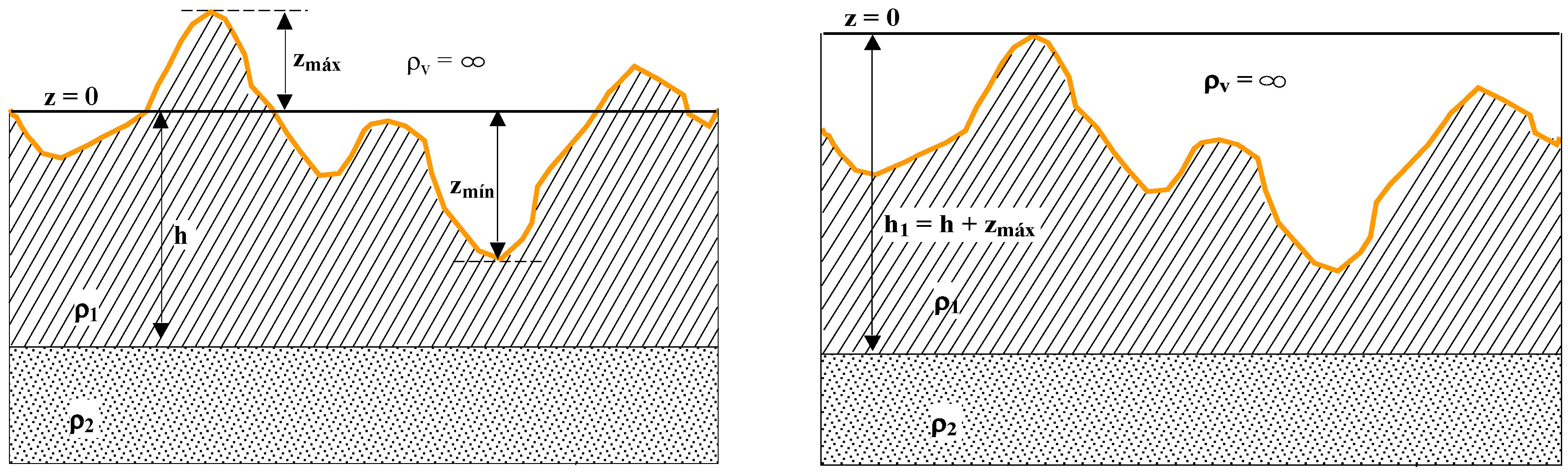
Non-planar soil surfaces can be treated in case of the unevenness at small-scale of length is not significant and in addition, the amplitude of the unevenness is much smaller than the size of the measuring area (an almost-flat surface) [4,5]. However, the lack of flatness in the soil surface could lead to significant differences in the grounding resistance with respect to a flat surface. When irregularities also occur on a small scale on the surface, i.e., at the electrode size scale, the grounding resistance measures may contain large errors which must be taken into account in the design stage of the protection system of the electrical installation. In this work, the influence of an uneven soil surface on the measurement of grounding resistance is studied. The irregularity will occur on all spatial scales with a maximum intensity to be controlled in this study. For this purpose, a fractal landscape generator will be used and the resulting surface will be suitably meshed to use the boundary elements method (BEM) [6] in the calculations. From a multi-layered soil with such an uneven surface, the grounding resistance of a proposed electrode is evaluated.

For this purpose, the paper is organized as follows. After this introduction, the soil model, along with its irregular surface and the theoretical foundation underlying all the calculations, is presented in Section 2. In Section 3, the results of the grounding resistance calculations are shown. Finally, Section 4 presents the final conclusions of this work.

2. Modeling the Uneven Soil Surface, Theoretical Background

2.1. Remodeling the Layers

We started with an initially flat N-layered soil, originally having ${\left\{{\rho }_i,h_i\right\}}_{i=1\dots N}$ parameters, whose surface is distorted to form an uneven landscape. The top layer was modified to include, in some way, the unevenness of the surface. Assuming that in the whole area of measurement, the maximum difference of the level in the surface was ${\Delta }_{\max }=Z_{\max }-Z_{\min }$, Z_max and Z_min being, respectively, the maximum and minimum level with respect to the initial flat surface, the top layer then was widened to a thickness of $h_1+Z_{\max }$ having a flat surface and the same resistivity ${\rho }_1$ as the old top layer. Note that the irregular ground surface remained inside the new top layer and the volume limited by the uneven surface and the flat surface of the new top layer was considered as an embedded volume of air embedded in this new and wider top layer. Figure 1 illustrates the model described, applied to an initial two-layered model.

Thus, an initially N-layered soil resulted in a new N-layered soil with a wider top layer inside, where there was located an embedded volume of very high resistivity representing the contribution of the uneven soil surface in the real soil model. Although the volume embedded in the top layer is not finite, only a finite portion of such a volume around the electrode system contributes significantly to the potential value. As a validation test of the proposed model, it will be seen later that if ${\Delta }_{\max }\to 0$, the model asymptotically gives the same numerical results corresponding to a perfectly flat surface with the same layer structure as the unmodified initial N-layered flat soil.

2.2. Theoretical Background

The potential profile, created by a system of conductors in mutual interaction, immersed in an electrically inhomogeneous medium, is the solution of Equation (1)

$$\overrightarrow{\nabla }\cdot (\sigma (\overrightarrow{r})\overrightarrow{\nabla }\varphi (\overrightarrow{r}))=0$$

(1)

in a 3D domain, where $\sigma (\overrightarrow{r})$ is the conductivity function and $\varphi (\overrightarrow{r})$ the potential that satisfies a set of boundary conditions which define univocally the configuration of the conductors, their electrical state and the properties of the inhomogeneous medium. The conductors may be independent or may be electrically interconnected. If the initial domain can be decomposed into several regions or volumes, for each region R of the domain where the conductivity is a constant, the equations that need to be solved are shown in Equation (2):

$$\begin{array}{c}{\overrightarrow{\nabla }}^2{\varphi }_R=0\hfill \\ {{\varphi }_R(\overrightarrow{r})|}_{\overrightarrow{r}\in S_{C_i}}=V_i\hfill \\ {\overrightarrow{n}\cdot \overrightarrow{\nabla }{\varphi }_R|}_G=0\hfill \\ {{\varphi }_R(\overrightarrow{r})|}_{\overrightarrow{r}\in S_I}={{\varphi }_{R^{\prime }}(\overrightarrow{r})|}_{\overrightarrow{r}\in S_I}\hfill \\ {{\sigma }_R\overrightarrow{\nabla }{\varphi }_R(\overrightarrow{r})\cdot \overrightarrow{n}|}_{\overrightarrow{r}\in S_I}={{\sigma }_{R^{\prime }}\overrightarrow{\nabla }{\varphi }_{R^{\prime }}(\overrightarrow{r})\cdot \overrightarrow{n}|}_{\overrightarrow{r}\in S_I}\hfill \end{array}$$

(2)

where $S_{C_i}$ stands for the surface of the $C_i$ conductor, the subscript G refers to the ground surface and $S_I$ stands for the interface between two media of different properties. The last two equations in Equation (2) express the continuity of both the electric potential and the current density flow through the interface $S_I$, separating the R and R′ regions of the constant conductivities ${\sigma }_R$ and ${\sigma }_{R^{\prime }}$. The vector $\overrightarrow{n}$ is a unitary vector normal to $S_I$ along R-R′.

If the soil is composed of layers separated by flat interfaces, Equation (2) can be solved using cylindrical coordinates and the separation of variables [7]. Consider, for instance, a two-layered soil where ${\rho }_1$ is the resistivity of the upper layer which has a thickness h, and ${\rho }_2$ is the resistivity of the lower layer. For a current point in the upper layer at $\left(x^{\prime },y^{\prime },z\prime \right)$ (source point), it can be shown that the potential generated at any point $\left(x,y,z\right)$ (field point) of this upper layer is given by Equation (3):

$$\begin{array}{c}{\varphi }_{11}(x,y,z;x^{\prime },y^{\prime },z^{\prime })=\frac{{\rho }_{1}I}{4\pi }\cdot \frac{1}{\sqrt{r^2+{(z-z^{\prime })}^2}}+\frac{{\rho }_{1}I}{4\pi }\cdot \frac{1}{\sqrt{r^2+{(z+z^{\prime })}^2}}\hfill \\ +\frac{{\rho }_{1}I}{4\pi }\cdot {\displaystyle \underset{0}{\overset{\infty }{\int }}2\frac{Cosh(\lambda (z-z^{\prime }))+Cosh(\lambda (z+z^{\prime }))}{1-k{e}^{-2\lambda h}}}k{e}^{-2\lambda h}{J}_0(\lambda r)d\lambda \hfill \end{array}$$

(3)

where $r=\sqrt{{(x-x^{\prime })}^2+{(y-y^{\prime })}^2}$ and $k=\frac{{\rho }_2-{\rho }_1}{{\rho }_2+{\rho }_1}$ is the so-called reflection coefficient between the two material layers. The $J_0$ function accounts for the first kind zero-order Bessel function. We will use the notation ${\varphi }_{ij}$ here for the potential in the j-layer by a point source in the i-layer. To deal with problems in which active electrodes are located in the two layers of the soil, expressions such as ${\varphi }_{12},{\varphi }_{21}$ and ${\varphi }_{22}$ will be needed, as shown in Equation (4):

$$\begin{array}{c}{\varphi }_{12}(x,y,z;x^{\prime },y^{\prime },z^{\prime })=\frac{{\rho }_{1}I}{4\pi }\cdot {\displaystyle \underset{0}{\overset{\infty }{\int }}\frac{(1+k)(1+e^{-2\lambda z^{\prime }})}{1-k{e}^{-2\lambda h}}}{e}^{-\lambda (z-z^{\prime })}{J}_0(\lambda r)d\lambda \hfill \\ {\varphi }_{21}(x,y,z;x^{\prime },y^{\prime },z^{\prime })=\frac{{\rho }_{2}I}{4\pi }\cdot {\displaystyle \underset{0}{\overset{\infty }{\int }}\frac{(1-k)(1+e^{-2\lambda z})}{1-k{e}^{-2\lambda h}}}{e}^{\lambda (z-z^{\prime })}{J}_0(\lambda r)d\lambda \hfill \\ {\varphi }_{22}(x,y,z;x^{\prime },y^{\prime },z^{\prime })=\frac{{\rho }_{2}I}{4\pi }\cdot \frac{1}{\sqrt{r^2+{(z-z^{\prime })}^2}}+\frac{{\rho }_{2}I}{4\pi }\cdot {\displaystyle \underset{0}{\overset{\infty }{\int }}\frac{(1-k{e}^{2\lambda h})}{1-k{e}^{-2\lambda h}}}{e}^{-2\lambda z^{\prime }}\cdot e^{-\lambda (z-z^{\prime })}{J}_0(\lambda r)d\lambda \hfill \end{array}$$

(4)

Note that in the above expressions, an improper integral is evaluated, which, when evaluated numerically, will cause unavoidable truncation errors that need to be controlled.

The electrodes buried in the soil acting as current sources are modeled as thin wire electrodes. For a curved thin wire of length L and radius r (L >> r) buried in the ground, the absolute potential at any point is calculated by assuming that there exists a continuous distribution of current points $\mu (x^{\prime },y^{\prime },z^{\prime })$ on the wire axis so that

$$\begin{array}{c}{\varphi }_{11}(x,y,z)=\frac{{\rho }_{1}I}{4\pi }\cdot {\displaystyle \underset{L}{\int }\frac{\mu (x^{\prime },y^{\prime },z^{\prime })}{\sqrt{r^2+{(z-z^{\prime })}^2}}}d{l}^{\prime }+\frac{{\rho }_{1}I}{4\pi }\cdot {\displaystyle \underset{L}{\int }\frac{\mu (x^{\prime },y^{\prime },z^{\prime })}{\sqrt{r^2+{(z+z^{\prime })}^2}}}d{l}^{\prime }+\hfill \\ \frac{{\rho }_{1}I}{4\pi }\cdot {\displaystyle \underset{L}{\int }\left[{\displaystyle \underset{0}{\overset{\infty }{\int }}2\frac{Cosh(\lambda (z-z^{\prime }))+Cosh(\lambda (z+z^{\prime }))}{1-k{e}^{-2\lambda h}}}k{e}^{-2\lambda h}{J}_0(\lambda r)d\lambda \right]}\mu (x^{\prime },y^{\prime },z^{\prime })d{l}^{\prime }\hfill \end{array}$$

(5)

The integral Equation (5) is solved using the method of moments [8,9]. Thin wires are then divided into M segments in which µ is a constant and a linear system is obtained while the electrode is at equipotential. In Equation (6), the img superscript refers to magnitudes measured on the image electrode and $r=\sqrt{{(x_{i,j}-x_{n,m})}^2+{(y_{i,j}-y_{n,m})}^2}$ since current points on the real and image electrodes only differ in the z coordinate.

$$\begin{array}{c}{V}_{ij}={\displaystyle \sum _{n,m}{\mu }_{l_{n,m}}\left({\displaystyle \underset{L_{n,m}}{\int }\frac{{\rho }_{1}d{l}_{n,m}}{4\pi \left|{\overrightarrow{r}}_{i,j}-{\overrightarrow{r}}_{n,m}\right|}+{\displaystyle \underset{L_{n,m}}{\int }\frac{{\rho }_{1}d{l}_{n,m}^{img}}{4\pi \left|{\overrightarrow{r}}_{i,j}-{\overrightarrow{r}}_{n,m}^{img}\right|}}}\right)}+\hfill \\ {\displaystyle \sum _{n,m}{\mu }_{l_{n,m}}\left({\displaystyle \underset{L_{n,m}}{\int }\frac{{\rho }_1}{4\pi }\left[{\displaystyle \underset{0}{\overset{\infty }{\int }}2\frac{Cosh(\lambda (z_{i,j}-z_{n,m}))+Cosh(\lambda (z_{i,j}-z_{n,m}^{img}))}{1-k{e}^{-2\lambda h}}}k{e}^{-2\lambda h}{J}_0(\lambda r)d\lambda \right]}d{l}_{n,m}\right)}\hfill \end{array}$$

(6)

Index i and j in Equation (6) appoint to the conductor i and segment j, respectively, and $V_{ij}=V_i$ for all segments j of the conductor i fulfilling the equipotential requirement. Similarly, index n and m in Equation (6) refer to the contribution of the conductor n and segment m to the potential $V_{ij}$. We emphasize that Equations (3)–(6) are only valid for two-layered soil models, and can be extended to multi-layered soil without difficulty. In general, to deal with N-layered soil, it is necessary to start from a set of equations, such as those shown in Equation (7):

$${\varphi }_{ij}(x,y,z;x^{\prime },y^{\prime },z^{\prime })=\frac{{\rho }_{i}I}{4\pi }{\displaystyle \underset{0}{\overset{\infty }{\int }}\left[e^{-\lambda \left|z-z^{\prime }\right|}\cdot {\delta }_{ij}+f_{ij}\cdot e^{-\lambda (z-z^{\prime })}+g_{ij}\cdot e^{\lambda (z-z^{\prime })}\right]}{J}_0(\lambda r)d\lambda$$

(7)

where $i,j=\mathrm{1...}N$, ${\delta }_{ij}$ is the Kronecker symbol and $f_{ij}$, $g_{ij}$ are functions to be calculated by imposing the boundary conditions given in the last three equations in Equation (2).

It only remains to include in this scheme the contribution of any volume embedded in the layers which has a different resistivity ${\rho }_v$ than the surrounding bulk. The uneven surface is considered as an interface of an embedded volume in the upper layer of the model. This volume is a horizontal infinite layer whose upper boundary is the flat surface of the new soil model, and its lower boundary is the uneven surface of the real soil, as shown in Figure 1. The contribution to the potential is done by the equivalent surface charge distributions (ESCD) approach [10,11,12], which assumes the existence of a charge density on the volume interfaces, whose value is determined during the calculation. The potential associated with ESCD should be included as a contribution to the total potential on the electrodes, which also must satisfy the boundary conditions included in the last two equations in Equation (2). Equation (8) shows the contribution of the ESCD to the potential and fulfillment of the boundary conditions imposed,

$$\begin{array}{c}{\displaystyle \sum _{n,m}{\mu }_{l_{n,m}}{\displaystyle \underset{L_{n,m}}{\int }\frac{{\rho }_{1}d{l}_{n,m}}{4\pi \left|{\overrightarrow{r}}_{i,j}-{\overrightarrow{r}}_{n,m}\right|}}+{\displaystyle \sum _t{\mu }_{I_t}{\displaystyle \underset{I_t}{\int }\frac{d{S}_t}{4\pi \epsilon \left|{\overrightarrow{r}}_{i,j}-{\overrightarrow{r}}_t\right|}}}+IMAGES}=V_{ij}\hfill \\ {\mu }_{I_s}+2K\left[{\displaystyle \sum _{n,m}{\mu }_{l_{n,m}}{\displaystyle \underset{L_{n,m}}{\int }\frac{{\rho }_1}{4\pi }\overrightarrow{\nabla }(\frac{1}{\left|{\overrightarrow{r}}_{n,m}-{\overrightarrow{r}}_s\right|})\cdot \overrightarrow{n}d{l}_{n,m}}}+{\displaystyle \sum _{t\ne s}{\mu }_{I_t}{\displaystyle \underset{I_t}{\int }\frac{1}{4\pi \epsilon }\overrightarrow{\nabla }(\frac{1}{\left|{\overrightarrow{r}}_s-{\overrightarrow{r}}_t\right|})\cdot \overrightarrow{n}d{S}_t}}+IMAGES\right]=0\hfill \end{array}$$

(8)

where $K=\frac{{\rho }_v-{\rho }_1}{{\rho }_v+{\rho }_1}$ and the s and t indices range along the patches $I_t$ in which the uneven surface should be divided, for instance by a triangular meshing whose outgoing normal vectors are $\overrightarrow{n}$. As the uneven surface really is infinite, this contribution is taken into account from the partial meshing of the surface, which is carried out in a circular area, centered on the electrode system, with a radius equal or higher than 3L_c, L_c being the characteristic length of the electrode system. This lower bound for the meshing radius has been determined by the authors using numerical experiments with simple electrodes of various sizes.

Figure 2 illustrates some of the magnitudes contained in Equation (8) and refers to the contribution to the potential of segment j of conductor $C_i$, named $L_{i,j}$, due to the interface triangular patch $I_t$. The normal vector $\overrightarrow{n}$ to the $I_t$ patch is also represented.

It is assumed that the charge density ${\mu }_{I_t}$ on each patch is uniform. In Equation (8), the term IMAGES includes all contributions due to the images relative to the soil surface. Also included are images due to the multi-layered soil structure as in Equation (6). The set of Equation (8) is completed with the condition imposed on the sum of the currents filtered by the electrodes. This sum must be equal to the initially known total current I injected into the system, as shown in Equation (9).

$${\displaystyle \sum _{n.m}{\mu }_{l_{n,m}}\cdot d{l}_{n,m}=I}$$

(9)

From Equation (8), we can formally define the impedance matrix $(Z_{\alpha \beta })$ of the linear system by $(V_{\alpha })=(Z_{\alpha \beta })({\mu }_{\beta })$, where vector $({\mu }_{\beta })$ includes the leakage current densities of the electrodes and the charge densities on the interface surfaces, and vector $(V_{\alpha })$contains the potentials of all the segments of the electrodes, and the rest of their elements are zero according to the second equation contained in Equation (8).

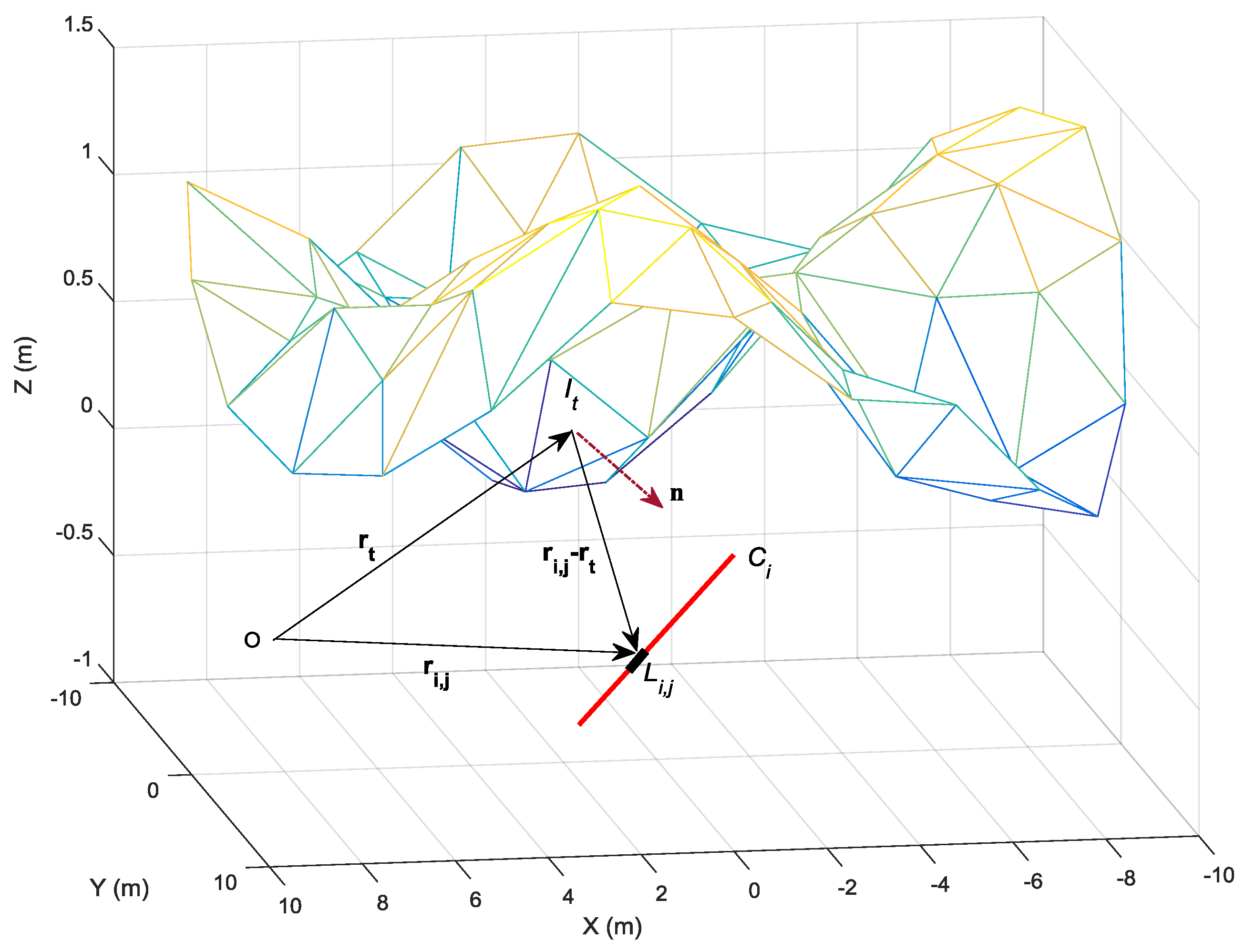
3. Stochastic Model for the Grounding Resistance

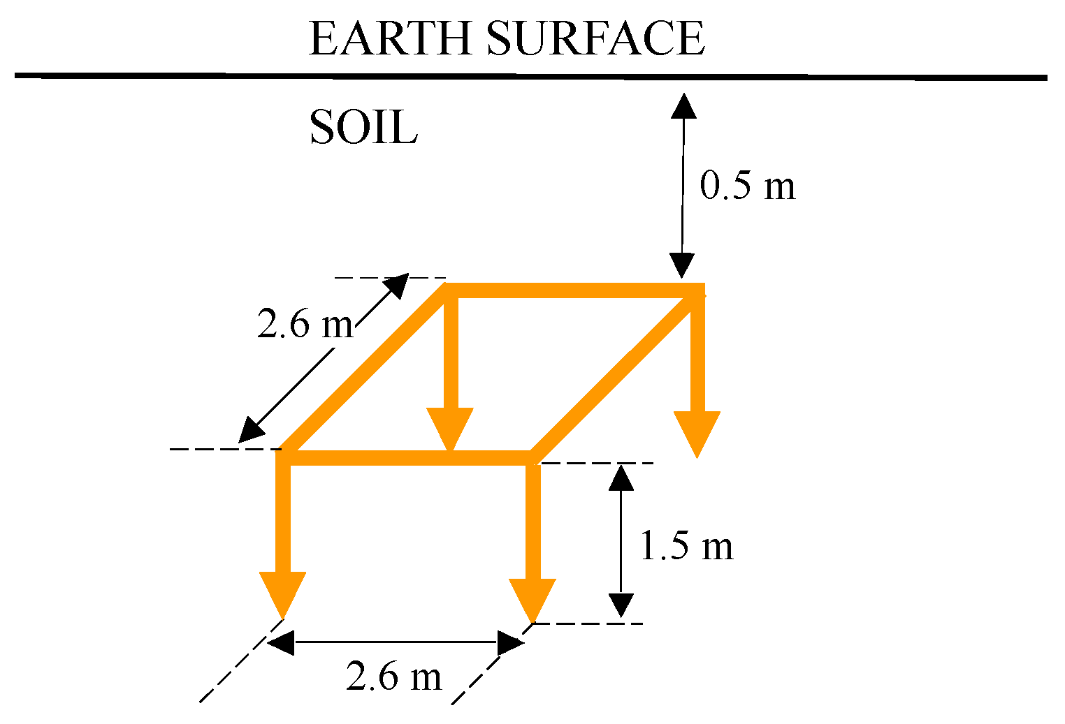
The theoretical model presented in Section 2 is to be applied to the calculation of the grounding resistance of a complex electrode, as shown in Figure 3, when the earth’s surface is uneven.

For this purpose, an uneven surface generator was used. The uneven surface chosen was built from a 2D fractal generator (FMW) based on the Mandelbrot-Weierstrass function [13,14]. The surface unevenness is associated with the variance of the stochastic process contained in the generator, not being allowed very extreme local values. The parameters defining the surface generated are H, the pseudo-Hurst exponent, which controls the correlation between adjacent data, and St, the unevenness strength. H values ranging from 0 to 1 generate very spiky surfaces, while H values >1 result in smoother surfaces which correspond to a strong correlation. Typical values used in this work were H = 1.2 and St = 0.1. As with any fractal structure, any portion of the generated surface has the same statistical properties of the entire surface, particularly the variability which is present at all length scales on the surface.

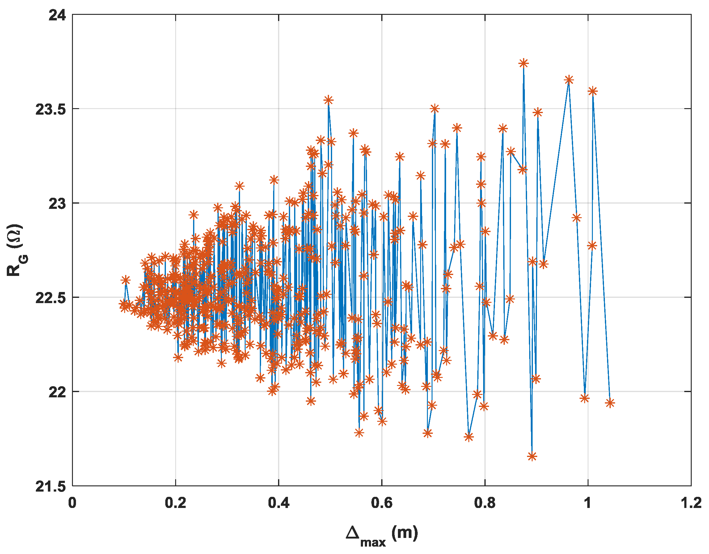
Using the FMW generator, a sample of 500 surfaces of two-layered soil characterized by ${\rho }_{1 }$= 200 Ω·m, ${\rho }_2$= 113 Ω·m, $h=2$ m were generated. These parameters will be referred to as the initial soil parameters and coincide with those measured at a place located in Madrid (Spain) used for electrical tests. The soils had a varied range of maximum unevenness between 0 < Δ_max < 1 m. For each generated soil, the grounding resistance of the electrode was calculated. 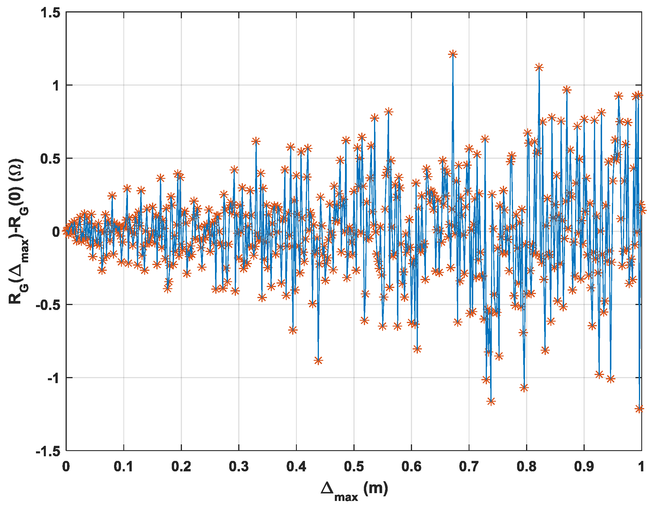Figure 4 shows the relationship between the grounding resistance R_G and the ground unevenness ${\Delta }_{\max }$. The great variability of the series, which presents increased intensity fluctuations as ${\Delta }_{\max }$ grows, can be seen.

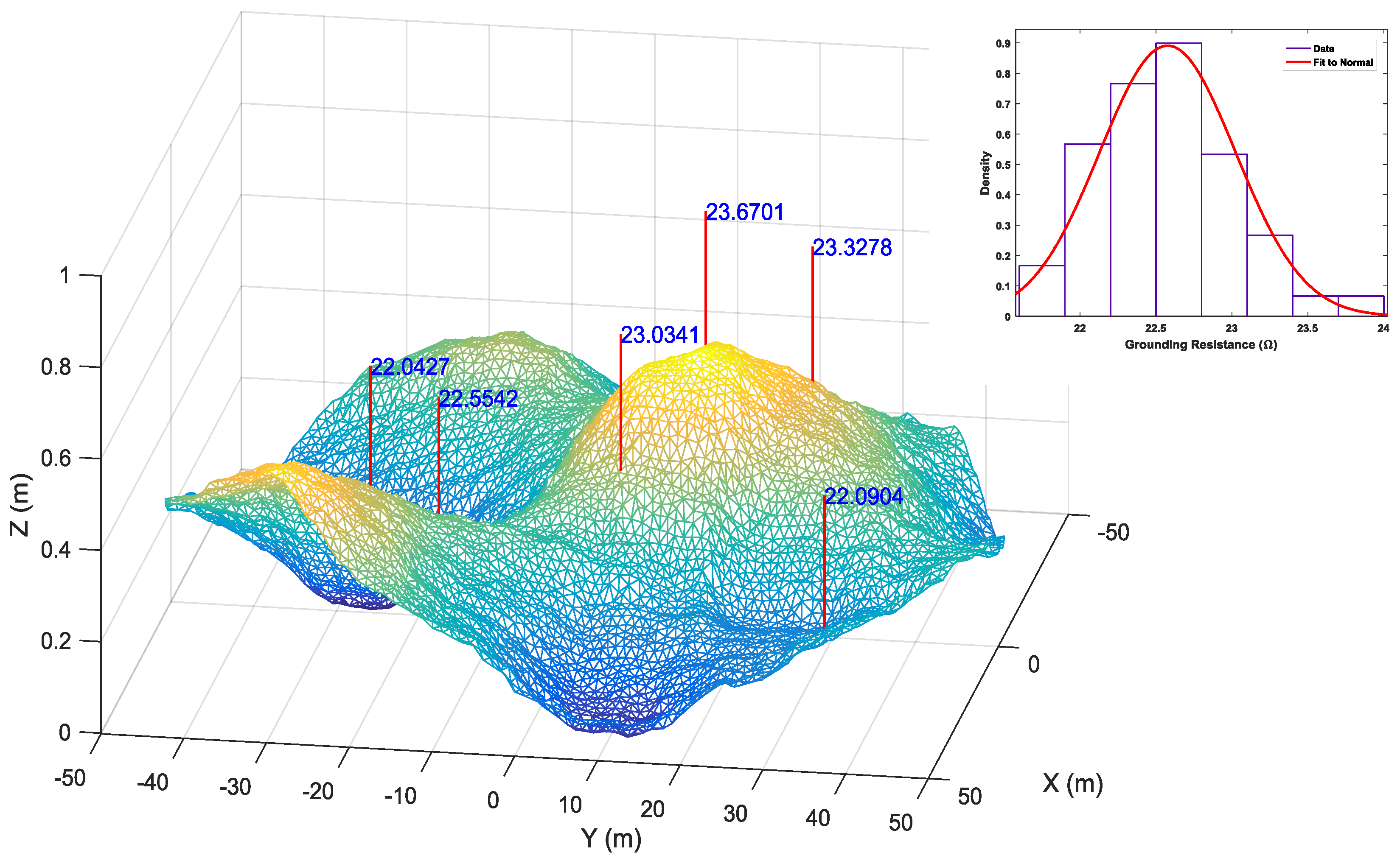
It should be noted that for a specific uneven surface, the ground resistance may vary considerably by moving the electrode horizontally, as shown in Figure 5, where the value of the electrode grounding resistance, when it was located at several different positions under the surface, is represented.

The subfigure of Figure 5 shows the distribution of the calculated grounding resistance values for a soil with ${\Delta }_{\max }$ = 0.5792 m when the electrode is placed in N = 100 different positions under the surface in a radius of 50 m. A fit to a normal distribution was performed, having a mean value 22.5 Ω, which approximately corresponds to the value of the electrode grounding resistance for a flat surface, which is set at 22.59 Ω. From Figure 4, the relationship between R_G and ${\Delta }_{\max }$ may be interpreted as a single realization of a stochastic process which may be characterized by the following properties: (a) it is a non-correlated process; (b) it is stationary in mean with a value of $\langle R_G\rangle ={\overline{R}}_G$ = 22.59 Ω, which correspond to the grounding resistance in a flat soil; (c) the variance is not constant but increases with ${\Delta }_{\max }$; (d) since it is built from the calculation of the grounding resistance in a soil with a self-similar surface, it must inherit some kind of self-similarity. The stochastic model R_G(${\Delta }_{\max }$) must explain the variability found in the R_G calculation and provide an estimate of the variance which can be used for estimating the uncertainty in the R_G measure in a rough soil characterized by the unevenness level ${\Delta }_{\max }$. In this paper it is proposed by the simple model:

$$R_G({\Delta }_{\max })-R_G(0)=\alpha \cdot {({\Delta }_{\max })}^{\beta }\epsilon ({\Delta }_{\max })$$

(10)

where α and β are constants to be determined, and $\epsilon ({\Delta }_{\max })$ is an uncorrelated noise whose structure and properties are deduced from the analysis of the distributions as the sub-figure of Figure 5. It will also be admitted that the random variable $\epsilon ({\Delta }_{\max })$ is normalized, that is with a zero mean and unit variance. Note that Equation (10) is stationary in mean but not in variance. The variance of this process is

$$\mathrm{var}(R_G({\Delta }_{\max })-R_G(0))={\alpha }^2\cdot {({\Delta }_{\max })}^{2\beta }$$

(11)

Figure 6 shows a realization of the stochastic process in Equation (1) when α = 1.0 and β = 1.2. If it is assumed that R_G(0) = 22.59 Ω, the series shown in Figure 4 and Figure 6 have a very similar general appearance, whenever it is taken into account that the series of Figure 6 was evenly sampled while that of Figure 4 was sampled according to the output of the FMW generator.

The actual values of the α and β parameters must be obtained from the variance of the R_G distributions associated with soils with a different unevenness level ${\Delta }_{\max }$.

Table 1. The central variance of normal R_G distributions versus the unevenness level ${\Delta }_{\max }$, from N = 100 samples.

$\mathrm{var}(R_G-{\overline{R}}_G)$	0.0217	0.0057	0.0443	0.0519	0.0949	0.2003	0.4061	0.7417
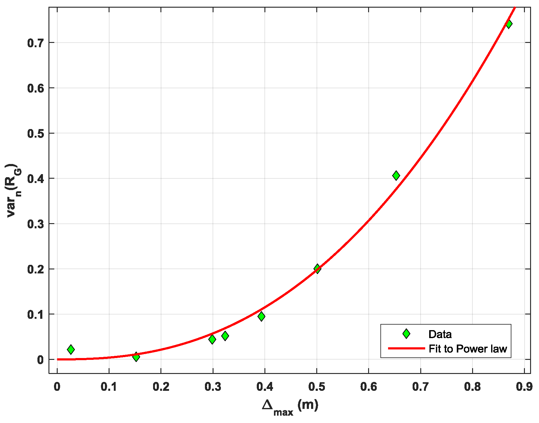
${\Delta }_{\max }$	0.0263	0.1521	0.2986	0.3235	0.3934	0.5013	0.6529	0.8695

shows the estimated central variance of the assumed normal R_G distributions from N = 100 random electrode positions under a surface of unevenness level ${\Delta }_{\max }$. From the results, the parameters can be obtained by fitting the central variance to a power law, $\mathrm{var}(R_G({\Delta }_{\max })-{\overline{R}}_G)=a\cdot {({\Delta }_{\max })}^b$.

Figure 7 shows such a fit procedure from which the values a = 1.055 ± 0.088 and b = 2.417 ± 0.263 are obtained. With respect to the coefficient b, note that its value is closely related to the H parameter since $b\approx 2H$, showing a clear connection between the surface soil structure and the measure the grounding resistance, so that finally, $\alpha =\sqrt{a}=1.0271$ and $\beta =\frac{b}{2}\cong 1.2=H$.

Thus, a value of uncertainty in the measurement of the grounding resistance for a soil with an uneven surface ${\Delta }_{\max }$ will be given by $R_G({\Delta }_{\max })\pm 3\sigma ({\Delta }_{\max })$, where σ stands for the standard deviation, which is given by the square root of Equation (11), $\sigma ({\Delta }_{\max })=\alpha \cdot {({\Delta }_{\max })}^H$, thus

$$R_G({\Delta }_{\max })\pm 3\cdot \alpha \cdot {({\Delta }_{\max })}^H$$

(12)

As an example, for a soil with ${\Delta }_{\max }=0.3$ m, then $\sigma =0.2388$ Ω and the uncertainty in R_G is 0.71 Ω, which corresponds to around 3% of the expected value for a flat soil, which is 22.59 Ω. However, this percentage increases to 6% if the unevenness becomes ${\Delta }_{\max }=0.5$ m. It should be remembered that ${\Delta }_{\max }$ is an overall measure of the unevenness associated with the portion of the surface soil that contributes to the grounding resistance calculation.

It should be taken into account that both parameters α and β in Equation (10) will depend on the properties of the multi-layered soil and possibly also on parameter H of the surface. This dependence can be investigated by numerical experiments with ${\rho }_1/{\rho }_2$, h and H as variables. With respect to β, the dependence on the soil and H parameters will have the general form $\beta =f\left({\rho }_1/{\rho }_2,h\right)·H$ if the soil fits into a monofractal model, while it will have the form $\beta =f\left({\rho }_1/{\rho }_2,h\right)·g\left(H\right)$ if the soil fits into a multifractal model. In both cases, the function $f\left({\rho }_1/{\rho }_2,h\right)$ can also be determined by numerical experiments while $g\left(H\right)$ is closely related to the multifractal spectrum of the uneven soil surface [15].

The application of these results to the real world must begin with the assumption of a model that reproduces the irregularity of the soil surface. With regard to self-similar models, as discussed here, there are methods that allow us to find the H parameter from a natural terrain [16]. With the calculation of the grounding resistance of a specific electrode from a flat soil surface, the actual resistance to be measured in the real terrain with a given maximum unevenness will have a confidence interval given by Equation (12) when the non-flat soil surface is considered as the only source of variability for the grounding resistance.

4. Conclusions

This paper has addressed the problem of evaluating the influence of the irregular surface of a soil on the measurement of the ground resistance of a complex electrode. For this purpose, a soil model was proposed, which allows the use of known calculation expressions only valid for flat soils. A large sample of multi-layered soils with irregular surfaces at all spatial scales, following the Mandelbrot-Weierstrass function with a driving parameter H, were generated. Soils were classified according to the intensity ${\Delta }_{\max }$ of their maximum unevenness level, and the grounding resistance of a specific electrode buried in the upper layer was calculated. From the results obtained, a stochastic model for grounding resistance as a function of the unevenness level was proposed. The model is stationary in mean but not in variance. The mean value coincides with the grounding resistance on a flat ground, while the variance follows an unevenness level power law. The exponent is closely related to that used in the process of generating the irregular surfaces, H. The standard deviation is given by $\sigma ({\Delta }_{\max })=\alpha \cdot {({\Delta }_{\max })}^H$, where α = 1.0271 and H = 1.2. Thus, by defining the uncertainty in determining the grounding resistance as $\Delta R_G({\Delta }_{\max })=3\cdot \sigma ({\Delta }_{\max })$, the error rate in the R_G measurement for each unevenness level can be easily estimated.

References

1. IEEE Guide for Safety in AC Substation Grounding; IEEE Std.: New York, NY, USA, 2000.
2. Meliopoulos, A.P.; Webb, R.P.; Joy, E.B. Analysis of grounding systems. IEEE Trans. Power Appar. Syst. 1981, 3, 1039–1048. [Google Scholar] [CrossRef]
3. Colominas, I.; Gomez-Calvino, J.; Navarrina, F.; Casteleiro, M. A general numerical model for grounding analysis in layered soils. Adv. Eng. Softw. Workstn. 2002, 33, 641–649. [Google Scholar] [CrossRef]
4. Loke, M.H.; Chambers, J.E.; Rucker, D.F.; Kuras, O.; Wilkinson, P.B. Recent developments in the direct-current geoelectrical imaging method. J. Appl. Geophys. 2013, 95, 135–156. [Google Scholar] [CrossRef]
5. Koefoed, O.; Mallick, K. Geosounding Principles: Resistivity Sounding Measurements; Elsevier Scientific Publishing Company: Amsterdam, The Netherlands, 1979. [Google Scholar]
6. Katsikadelis, J.T. Boundary Elements Theory and Applications; Elsevier Scientific Publishing Company: Oxford, UK, 2002. [Google Scholar]
7. Calixto, W.P.; Neto, L.M.; Wu, M.; Yamanaka, K.; Moreira, E.P. Parameter estimation of a horizontal multilayer soil using genetic algorithm. IEEE Trans. Power Deliv. 2010, 25, 1250–1257. [Google Scholar] [CrossRef]
8. Harrington, R.F. Field Computation by Moment Methods; IEEE Press: New York, NY, USA, 1993. [Google Scholar]
9. Gibson, W.C. The Method of Moments in Electromagnetics; Chapman & Hall: London, UK, 2008. [Google Scholar]
10. Faleiro, E.; Asensio, G.; Moreno, J.; Simón, P.; Denche, G.; García, D. Modelling and simulation of the grounding system of a class of power transmission line towers involving inhomogeneous conductive media. Electr. Power Syst. Res. 2016, 136, 154–162. [Google Scholar] [CrossRef]
11. Ma, J.; Dawalibi, F.P. Analysis of grounding systems in soils with finite volumes of different resistivities. IEEE Trans. Power Deliv. 2002, 17, 596–602. [Google Scholar] [CrossRef]
12. Canova, A.; Gruosso, G. 3D source simulation method for static fields in inhomogeneous media. Int. J. Numer. Meth. Eng. 2006, 70, 1096–1111. [Google Scholar] [CrossRef]
13. Ausloos, M.; Berman, D.H. A multivariate weierstrass-mandelbrot function. Proc. R. Soc. Lond. A 1985, 400, 331–350. [Google Scholar] [CrossRef]
14. Wu, J.-J. Characterization of fractal surfaces. Wear 2000, 239, 36–47. [Google Scholar] [CrossRef]
15. Souza, J.; Rostirolla, S.P. A fast MATLAB program to estimate the multifractal spectrum of multidimensional data: Application to fractures. Comput. Geosci. 2011, 37, 241–249. [Google Scholar] [CrossRef]
16. Arakawa, K.; Krotkov, E. Fractal modeling of natural terrain: Analysis and surface reconstruction with range data. CVGIP-Gr. Models Image Process. 1996, 58, 413–436. [Google Scholar] [CrossRef]
Figure 1. Illustration on how to convert a two-layered soil with an uneven surface into a new two-layered soil with flat surface in order to use the theoretical background proposed in the paper. The left panel displays the original soil configuration while the right panel displays changes made to the top layer as described in the text.
Energies 10 00176 g001
Figure 2. Illustration of part of the calculation method contained in Equation (8).
Energies 10 00176 g002
Figure 3. Electrode model composed by thin wires whose grounding resistance is calculated in this work.
Energies 10 00176 g003
Figure 4. Grounding resistance RG vs. the soil unevenness Δ max .
Energies 10 00176 g004
Figure 5. Grounding resistance in Ω of the electrode when it is buried at the position marked by the vertical line in a soil with Δ max = 0.5792 m. The sub-figure shows the grounding resistance distribution from N = 100 samples together with a fit to a normal distribution.
Energies 10 00176 g005
Figure 6. A realization of the stochastic process in Equation (10).
Energies 10 00176 g006
Figure 7. The normalized variance of the stochastic process in Equation (10) as a function of the unevenness Δ max from data of Table 1.
Energies 10 00176 g007