
Linear Formulation for Short-Term Operational Scheduling of Energy Storage Systems in Power Grids


Abstract
:1. Introduction
2. Linear Expression of ESS Technical Constraints
2.1. Charging/Discharging Efficiency
2.2. Output Power Limits
2.3. State-of-Charge
2.4. Total Energy Limits
3. Linear Objective Functions for Applications in Power Grid
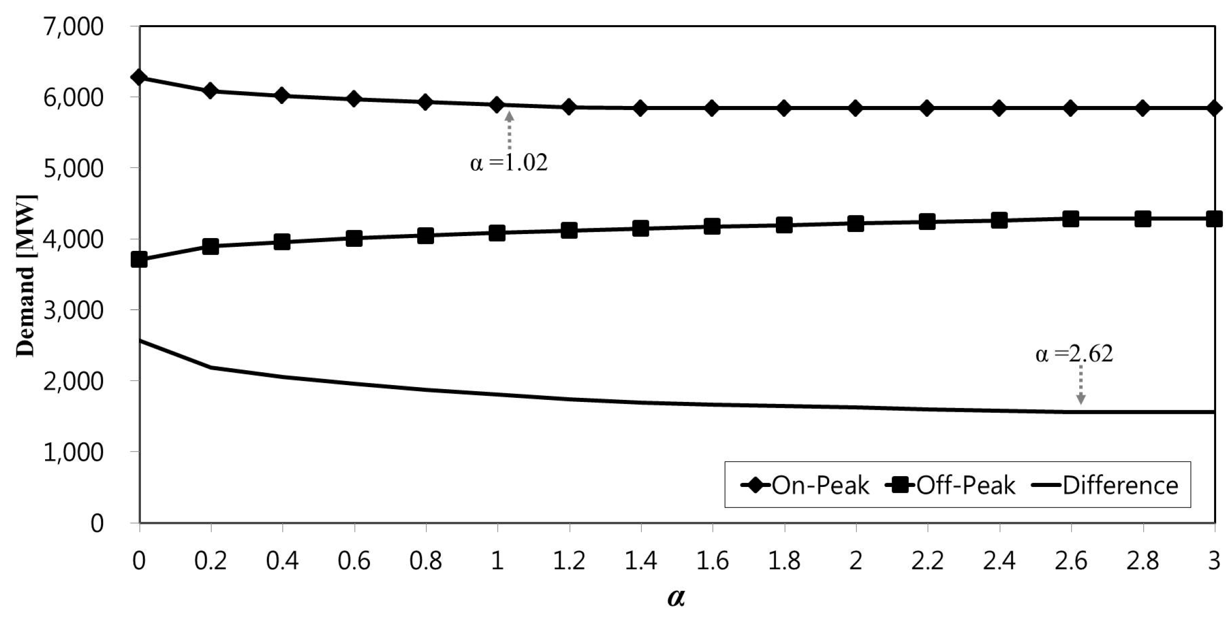
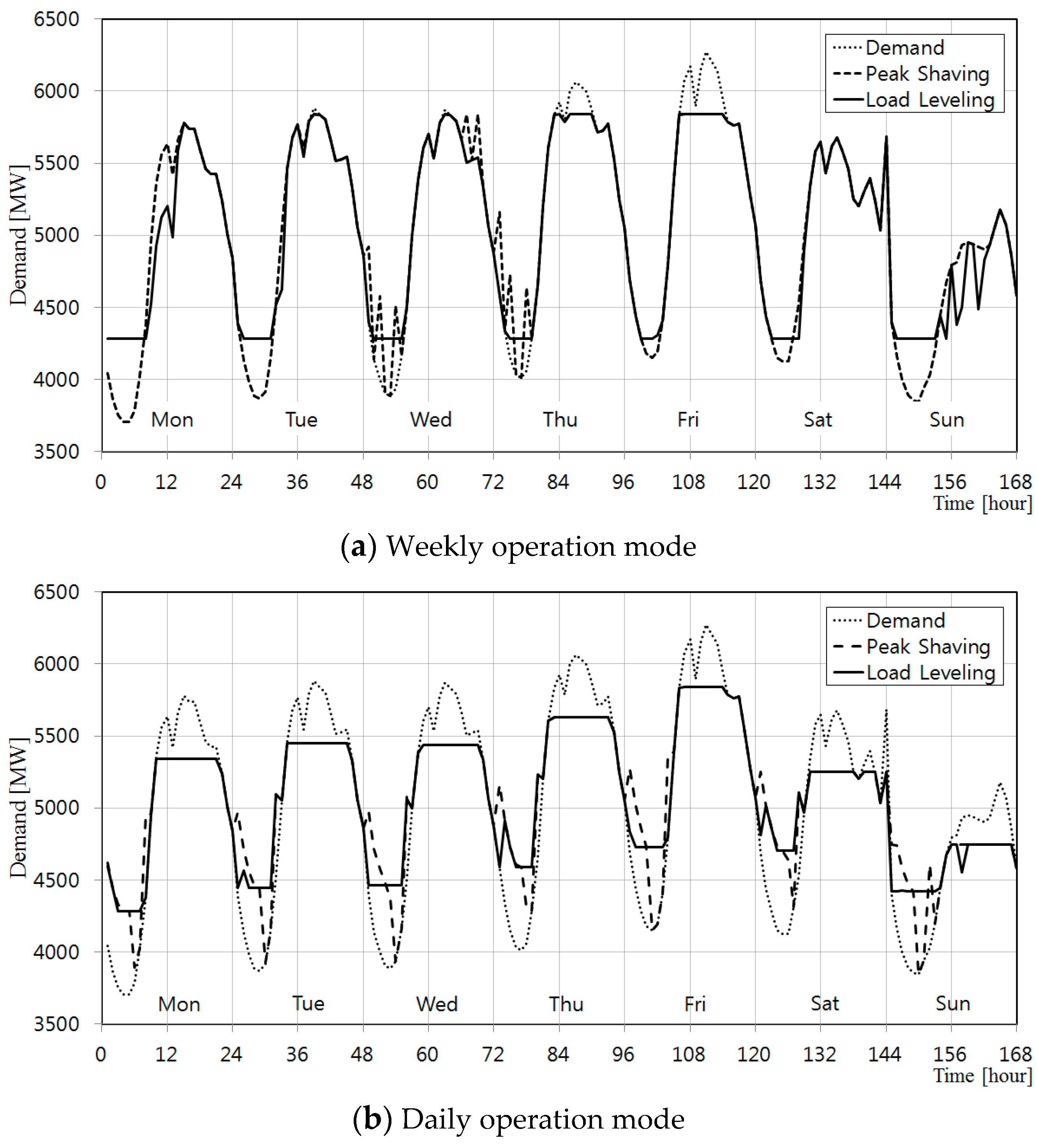
3.1. Peak-Shaving
3.2. Load-Leveling
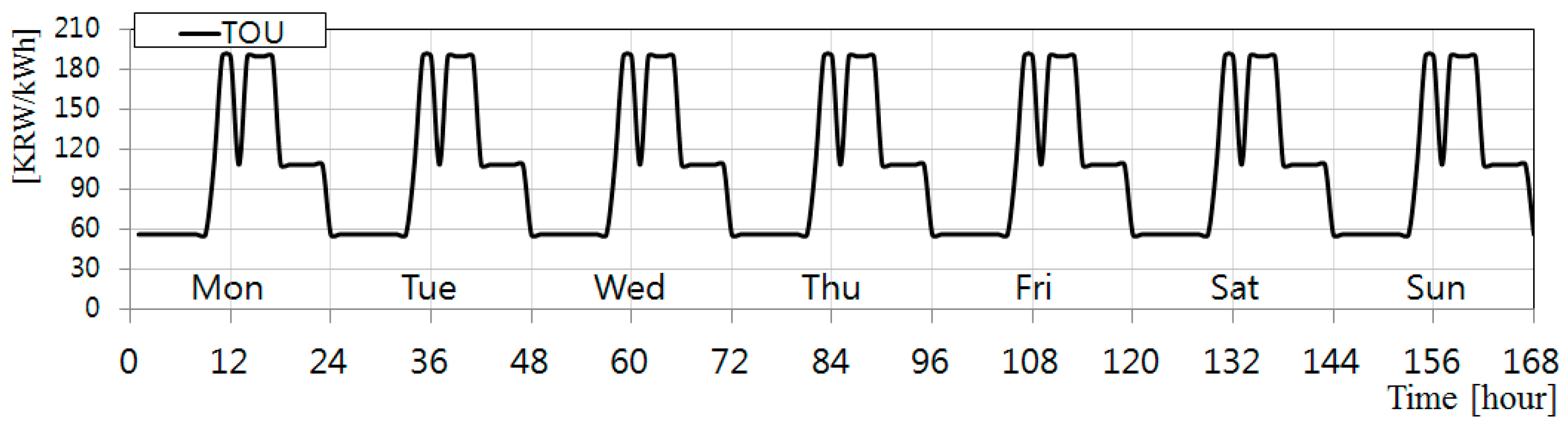
3.3. End-User Electricity Bill Minimization
4. Case Studies
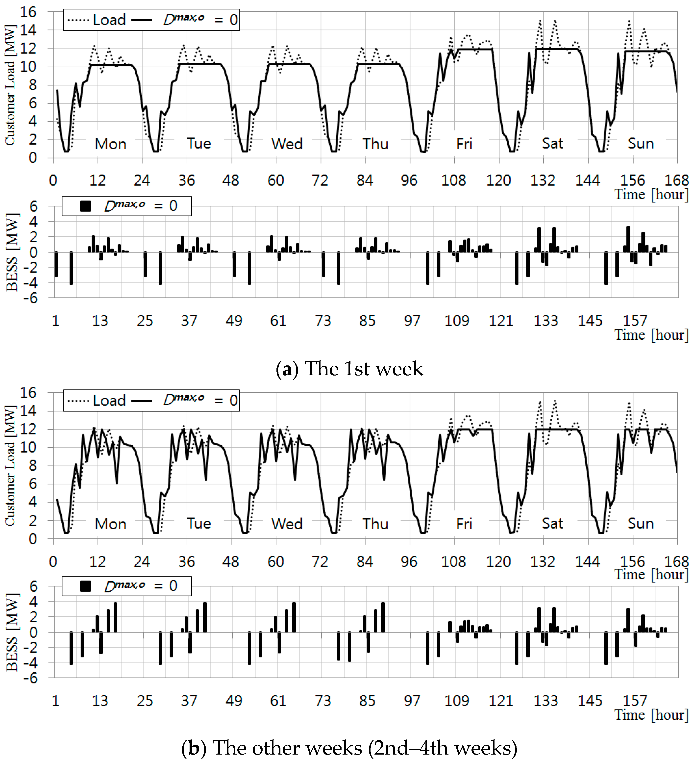
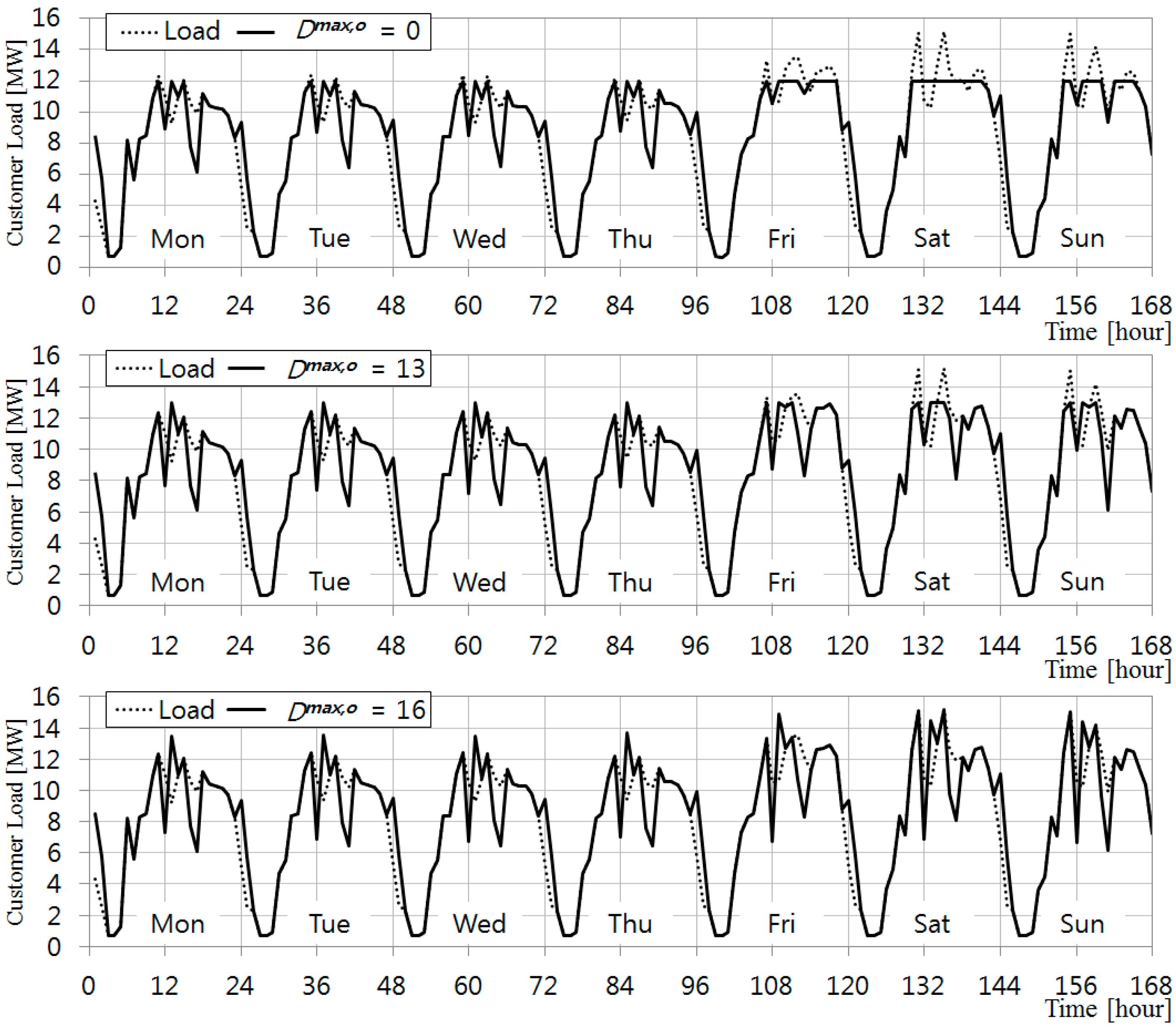
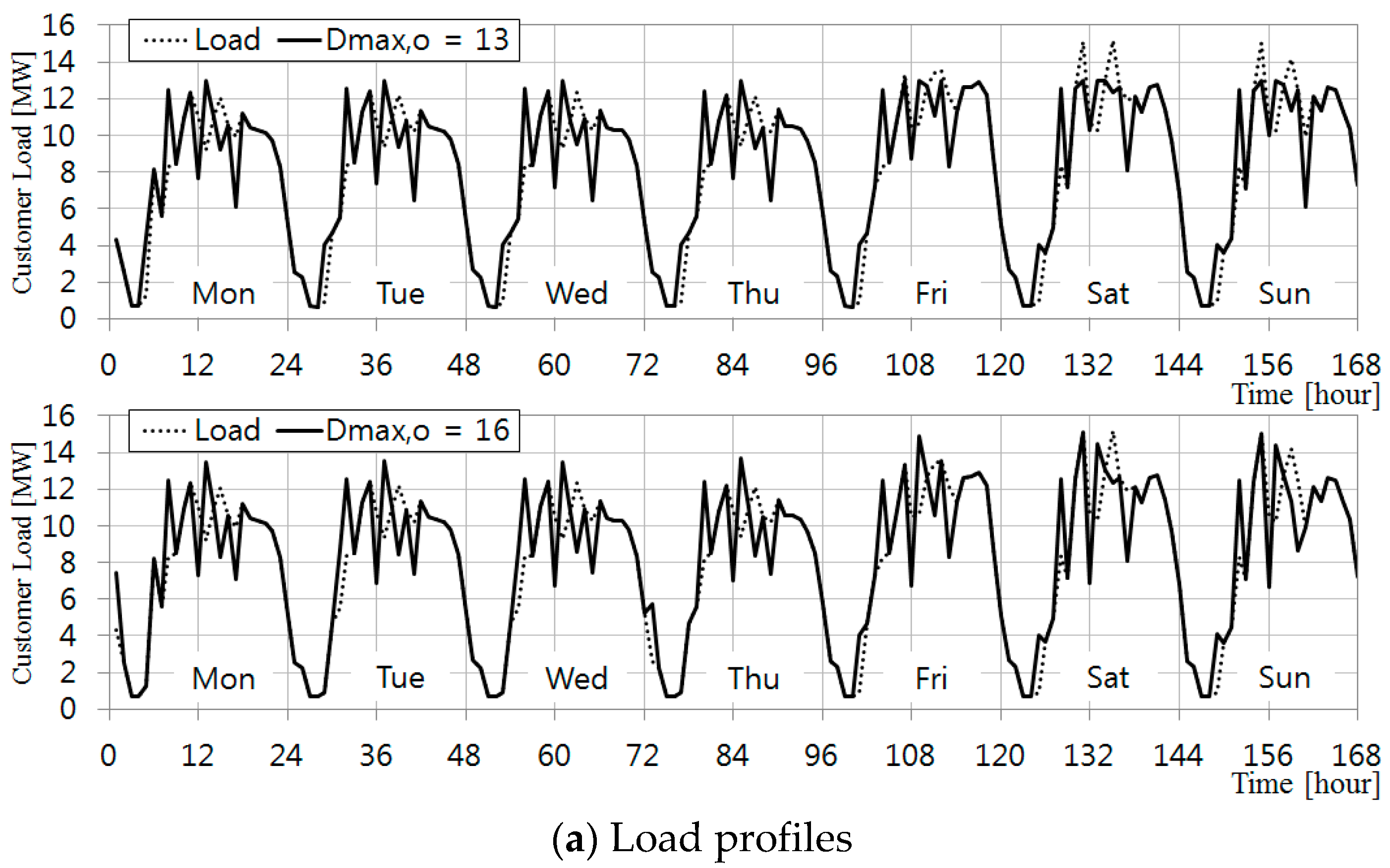
4.1. Case-I: Peak-Shaving and Load-Leveling with PHES
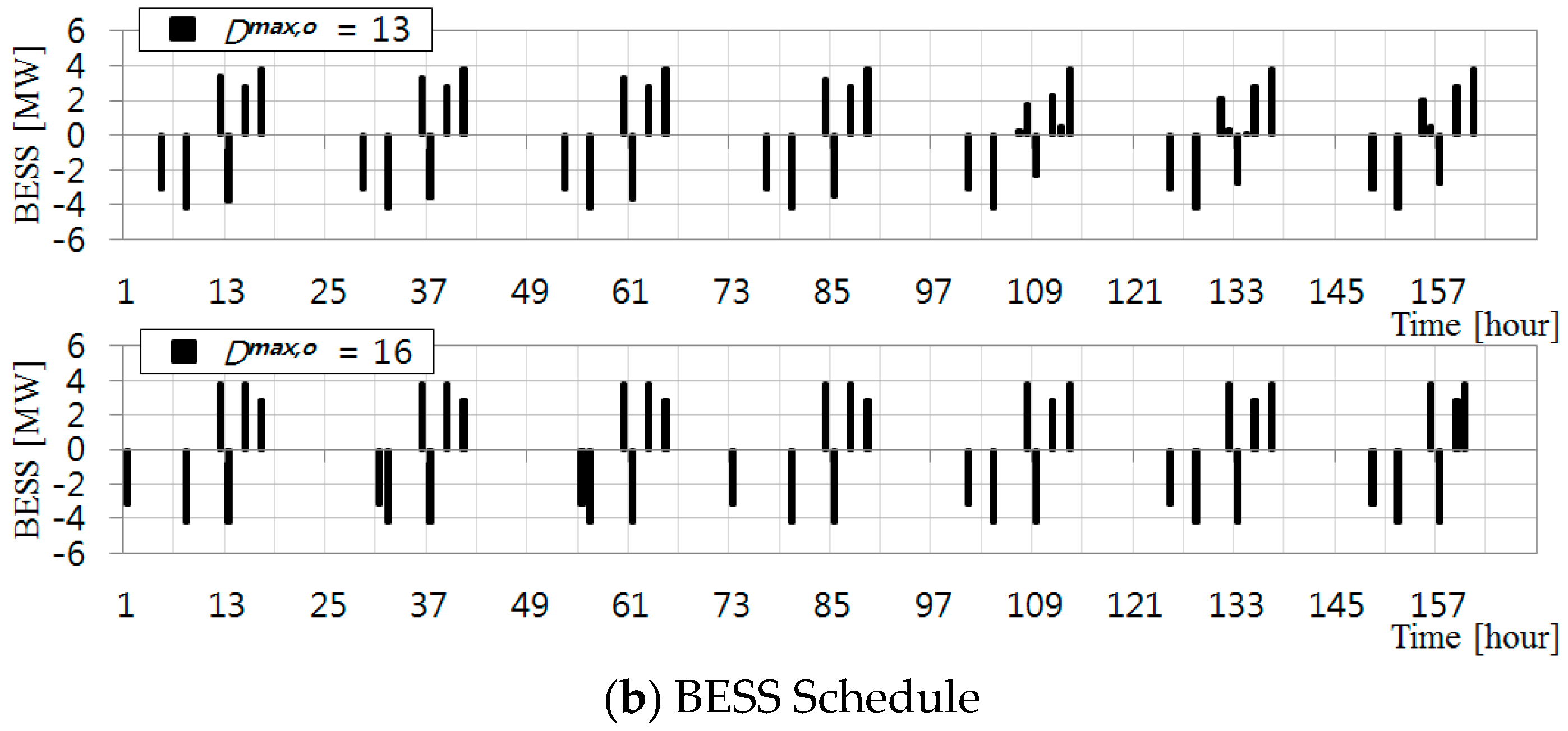
4.2. Case-II: Electric Bill Minimization of a Customer with Li-ion BESS
5. Conclusions
Author Contributions
Conflicts of Interest
Nomenclature
Indices
| Index of time intervals in a decision horizon T, | |
| Index of energy storage systems, |
Variables
| Adjusted demand by charging and discharging of ESSs at time interval-t | |
| The maximum demand with charging/discharging operation of ESSs during operating period (or the highest load to impose the demand charge in an end-user perspective) | |
| End-user’s historical maximum load | |
| The larger value between and | |
| The minimum demand with charging/discharging operation of ESSs | |
| Charging power of ESS-j from the grid at time interval-t | |
| Discharging power of ESS-j injected to the grid at time interval-t | |
| Charging power in ESS-j at time interval-t | |
| Discharging power from ESS-j at time interval-t | |
| State-of-charge of ESS-j at time interval-t | |
| Binary variable which is equal to 1 if ESS-j is under charge at time interval-t | |
| Binary variable which is equal to 1 if ESS-j is under discharge at time interval-t |
Constants
| A positive constant to limit the number of charging cycles of ESS-j during the operation period | |
| A positive constant to limit the number of discharging cycles of ESS-j during the operation period | |
| Estimated demand at time interval-t | |
| Minimum charging power of ESS-j | |
| Maximum charging power of ESS-j | |
| Minimum discharging power of ESS-j | |
| Maximum discharging power of ESS-j | |
| Power production of renewable resource at time interval-t | |
| Energy price at time interval-t | |
| Demand price imposed on of end-user | |
| Initial state-of-charge of ESS-j | |
| Maximum state-of-charge limit of ESS-j | |
| Minimum state-of-charge limit of ESS-j | |
| Lower bound of the state-of-charge of ESS-j at final time interval-T | |
| Upper bound of the state-of-charge of ESS-j at final time interval-T | |
| Charging efficiency of ESS-j | |
| The time interval unit in hours | |
| Discharging efficiency of ESS-j |
Appendix A

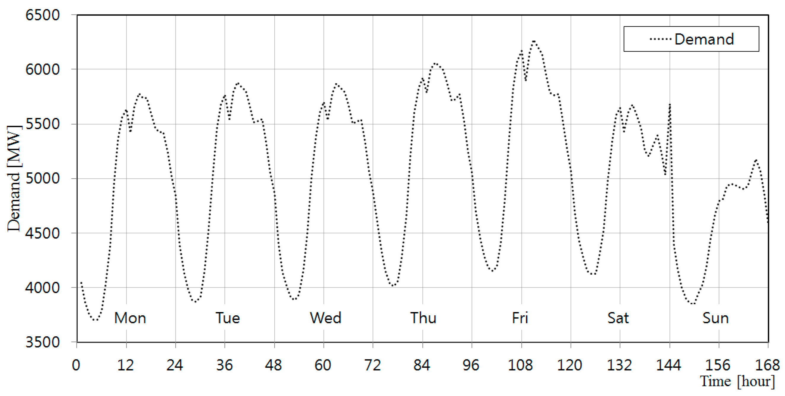
| Hour | Monday | Tuesday | Wednesday | Thursday | Friday | Saturday | Sunday |
|---|---|---|---|---|---|---|---|
| 1 | 4042 | 4389 | 4397 | 4586 | 4695 | 4688 | 4398 |
| 2 | 3864 | 4132 | 4141 | 4339 | 4439 | 4441 | 4161 |
| 3 | 3756 | 3984 | 4003 | 4152 | 4281 | 4273 | 4004 |
| 4 | 3707 | 3886 | 3904 | 4033 | 4183 | 4154 | 3895 |
| 5 | 3707 | 3866 | 3885 | 4014 | 4153 | 4125 | 3855 |
| 6 | 3787 | 3915 | 3934 | 4063 | 4193 | 4125 | 3845 |
| 7 | 4024 | 4153 | 4161 | 4281 | 4411 | 4312 | 3943 |
| 8 | 4380 | 4518 | 4507 | 4656 | 4796 | 4529 | 4031 |
| 9 | 4956 | 5054 | 5001 | 5201 | 5391 | 4966 | 4198 |
| 10 | 5361 | 5459 | 5386 | 5607 | 5836 | 5343 | 4445 |
| 11 | 5559 | 5677 | 5604 | 5835 | 6074 | 5580 | 4673 |
| 12 | 5638 | 5766 | 5703 | 5924 | 6173 | 5649 | 4793 |
| 13 | 5418 | 5546 | 5534 | 5785 | 5894 | 5430 | 4812 |
| 14 | 5657 | 5794 | 5782 | 6004 | 6153 | 5619 | 4931 |
| 15 | 5777 | 5884 | 5872 | 6065 | 6273 | 5680 | 4951 |
| 16 | 5737 | 5835 | 5833 | 6035 | 6203 | 5590 | 4941 |
| 17 | 5738 | 5805 | 5794 | 5995 | 6143 | 5461 | 4921 |
| 18 | 5608 | 5666 | 5664 | 5875 | 5954 | 5251 | 4900 |
| 19 | 5459 | 5517 | 5504 | 5716 | 5784 | 5201 | 4931 |
| 20 | 5428 | 5527 | 5523 | 5725 | 5763 | 5299 | 5057 |
| 21 | 5427 | 5545 | 5541 | 5773 | 5772 | 5397 | 5177 |
| 22 | 5237 | 5327 | 5333 | 5525 | 5554 | 5239 | 5069 |
| 23 | 5012 | 5060 | 5065 | 5246 | 5277 | 5032 | 4862 |
| 24 | 4845 | 4863 | 4879 | 5050 | 5070 | 5684 | 4585 |
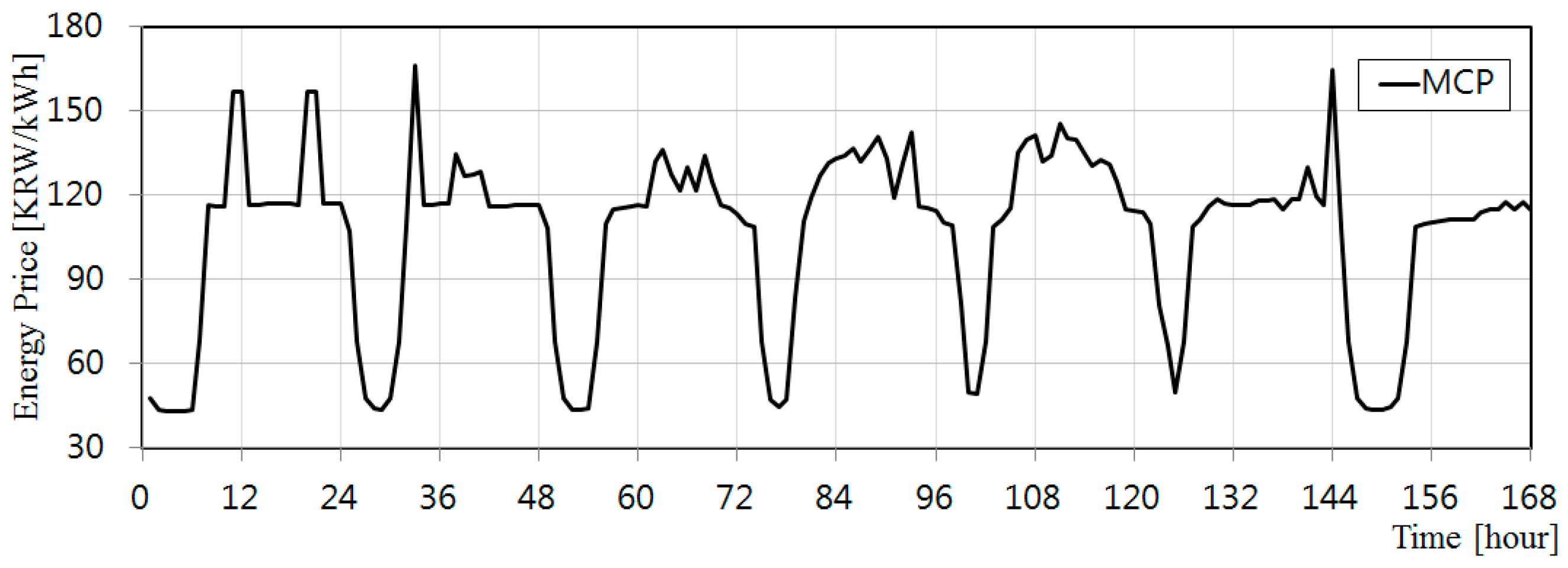
| Hour | Monday | Tuesday | Wednesday | Thursday | Friday | Saturday | Sunday |
|---|---|---|---|---|---|---|---|
| 1 | 47.61 | 107.38 | 108.24 | 110.12 | 110.53 | 113.8 | 108.25 |
| 2 | 43.89 | 68.20 | 68.2 | 108.71 | 109.41 | 109.67 | 68.21 |
| 3 | 43.39 | 47.55 | 47.57 | 67.91 | 81.53 | 80.76 | 47.58 |
| 4 | 42.97 | 43.93 | 43.92 | 47.45 | 49.77 | 66.60 | 44.24 |
| 5 | 42.97 | 43.73 | 43.92 | 44.74 | 49.59 | 49.66 | 43.89 |
| 6 | 43.42 | 47.55 | 44.17 | 47.45 | 67.83 | 68.02 | 43.74 |
| 7 | 68.30 | 68.20 | 68.20 | 83.30 | 109.01 | 108.66 | 44.53 |
| 8 | 116.47 | 109.45 | 109.95 | 110.68 | 111.27 | 111.38 | 47.58 |
| 9 | 116.31 | 166.42 | 114.91 | 119.27 | 115.53 | 115.92 | 68.21 |
| 10 | 116.31 | 116.37 | 115.60 | 127.04 | 135.38 | 118.47 | 108.62 |
| 11 | 157.06 | 116.62 | 116.17 | 131.60 | 140.13 | 117.02 | 109.94 |
| 12 | 157.06 | 117.11 | 116.35 | 133.27 | 141.37 | 116.86 | 110.34 |
| 13 | 116.53 | 117.11 | 116.12 | 133.96 | 132.38 | 116.86 | 111.05 |
| 14 | 116.53 | 134.78 | 132.21 | 136.75 | 134.39 | 116.77 | 111.22 |
| 15 | 117.32 | 127.10 | 136.08 | 131.89 | 145.79 | 117.98 | 111.65 |
| 16 | 117.32 | 127.53 | 127.66 | 136.10 | 140.57 | 118.17 | 111.65 |
| 17 | 117.32 | 128.68 | 121.64 | 141.06 | 139.94 | 118.55 | 111.65 |
| 18 | 117.32 | 116.12 | 130.11 | 133.22 | 134.49 | 115.10 | 114.21 |
| 19 | 116.37 | 116.15 | 121.64 | 118.97 | 130.72 | 118.70 | 115.15 |
| 20 | 157.06 | 116.30 | 133.94 | 131.64 | 132.79 | 118.70 | 115.20 |
| 21 | 157.06 | 116.47 | 124.92 | 142.26 | 131.34 | 130.29 | 117.78 |
| 22 | 116.99 | 116.47 | 116.49 | 116.04 | 125.12 | 119.78 | 115.20 |
| 23 | 116.99 | 116.47 | 115.63 | 115.41 | 115.12 | 116.82 | 117.77 |
| 24 | 116.99 | 116.47 | 113.4 | 114.68 | 114.66 | 164.46 | 114.84 |
| Demand Charge | 7380 (KRW/kW) | |||
|---|---|---|---|---|
| Energy Charge (KRW/kWh) | Time Period | Summer | Spring/Fall | Winter |
| Off-peak | 56.2 (23:00~09:00) | 56.2 (23:00~09:00) | 63.2 (23:00~09:00) | |
| Mid-peak | 108.5 (09:00~10:00, 12:00~13:00, 17:00~23:00) | 78.5 (09:00~10:00, 12:00~13:00, 17:00~23:00) | 108.5 (09:00~10:00, 12:00~17:00, 20:00~22:00) | |
| On-peak | 189.7 (10:00~12:00, 13:00~17:00) | 108.8 (10:00~12:00, 13:00~17:00) | 164.7 (10:00~12:00, 17:00~20:00, 23:00~23:00) | |
| Hour | Monday | Tuesday | Wednesday | Thursday | Friday | Saturday | Sunday |
|---|---|---|---|---|---|---|---|
| 1 | 4.29 | 2.54 | 2.70 | 2.58 | 2.64 | 2.68 | 2.58 |
| 2 | 2.56 | 2.27 | 2.27 | 2.27 | 2.31 | 2.30 | 2.30 |
| 3 | 0.69 | 0.69 | 0.68 | 0.69 | 0.68 | 0.69 | 0.69 |
| 4 | 0.68 | 0.66 | 0.66 | 0.67 | 0.66 | 0.70 | 0.68 |
| 5 | 1.28 | 0.90 | 0.90 | 0.91 | 0.88 | 0.89 | 0.91 |
| 6 | 8.19 | 4.67 | 4.70 | 4.69 | 4.69 | 3.64 | 3.58 |
| 7 | 5.60 | 5.54 | 5.49 | 5.58 | 7.27 | 4.98 | 4.42 |
| 8 | 8.27 | 8.35 | 8.38 | 8.20 | 8.28 | 8.37 | 8.29 |
| 9 | 8.47 | 8.53 | 8.38 | 8.47 | 8.48 | 7.15 | 7.08 |
| 10 | 10.92 | 11.26 | 11.07 | 10.80 | 10.83 | 12.53 | 12.43 |
| 11 | 12.32 | 12.40 | 12.39 | 12.18 | 13.31 | 15.10 | 15.01 |
| 12 | 11.06 | 10.69 | 10.49 | 10.84 | 10.52 | 10.69 | 10.47 |
| 13 | 9.24 | 9.33 | 9.30 | 9.45 | 10.66 | 10.25 | 10.22 |
| 14 | 10.99 | 11.01 | 10.80 | 10.99 | 12.72 | 13.06 | 12.74 |
| 15 | 12.07 | 12.23 | 12.36 | 12.14 | 13.41 | 15.15 | 14.19 |
| 16 | 10.55 | 10.82 | 10.95 | 10.46 | 13.54 | 12.63 | 12.46 |
| 17 | 9.90 | 10.23 | 10.25 | 10.22 | 12.11 | 11.89 | 9.92 |
| 18 | 11.18 | 11.34 | 11.35 | 11.43 | 11.31 | 12.13 | 12.14 |
| 19 | 10.41 | 10.48 | 10.43 | 10.53 | 12.63 | 11.29 | 11.38 |
| 20 | 10.27 | 10.37 | 10.30 | 10.53 | 12.66 | 12.62 | 12.60 |
| 21 | 10.16 | 10.22 | 10.29 | 10.33 | 12.93 | 12.75 | 12.51 |
| 22 | 9.73 | 9.77 | 9.75 | 9.74 | 12.21 | 11.42 | 11.26 |
| 23 | 8.32 | 8.41 | 8.39 | 8.53 | 8.81 | 9.72 | 10.35 |
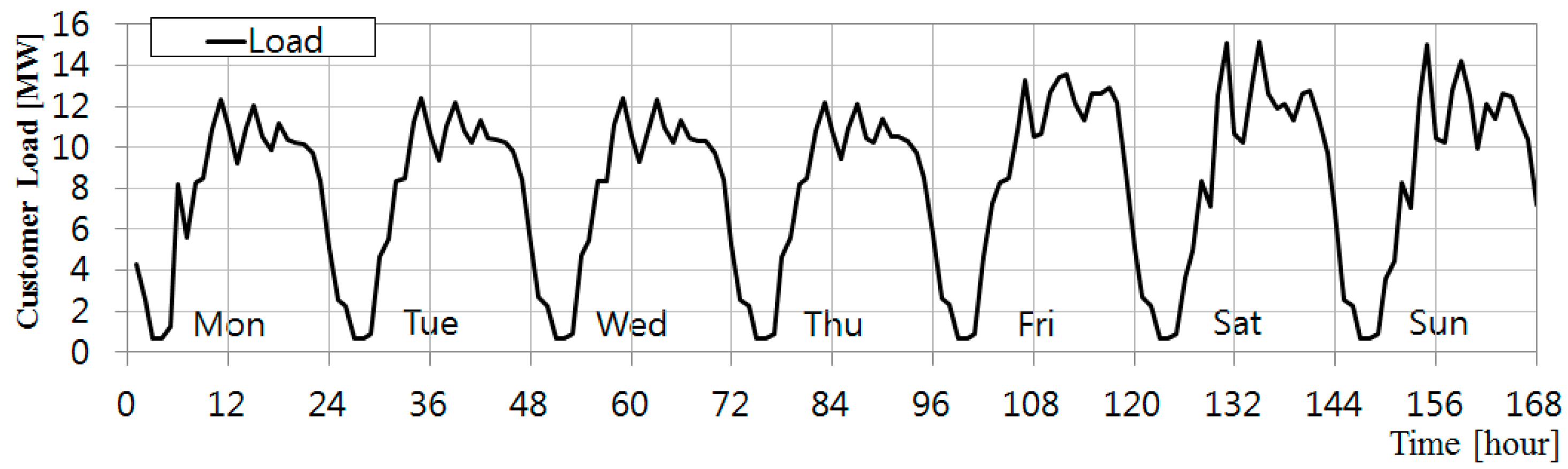
| 24 | 5.12 | 5.26 | 5.21 | 5.74 | 5.13 | 6.82 | 7.22 |
References
- Chen, H.; Cong, T.N.; Yang, W.; Tan, C.; Li, Y.; Ding, Y. Progress in electrical energy storage system: A critical review. Prog. Nat. Sci. 2009, 19, 291–312. [Google Scholar] [CrossRef]
- Akhil, A.A.; Huff, G.; Currier, A.B.; Kaun, B.C.; Rastler, D.M.; Chen, S.B.; Cotter, A.L.; Bradshaw, D.T.; Gauntlett, W.D. DOE/EPRI 2013 Electricity Storage Handbook in Collaboration with NRECA; Sandia Report No. SAND2013-5131; Sandia National Laboratories: Albuquerque, NM, USA, 2013.
- Sioshansi, R.; Denholm, P.; Jenkins, T.; Weiss, J. Estimating the value of electricity storage in PJM: Arbitrage and some welfare effects. Energy Econ. 2008, 31, 269–277. [Google Scholar] [CrossRef]
- Garcia-Gonzalez, J.; de la Muela, R.M.R.; Santos, L.M.; Gonzalez, A.M. Stochastic joint optimization of wind generation and pumped-storage units in an electricity market. IEEE Trans. Power Syst. 2008, 23, 460–468. [Google Scholar] [CrossRef]
- Mohamed, F. Microgrid Modelling and Online Management. Ph.D. Thesis, Helsinki University of Technology, Helsinki, Finland, 2008. [Google Scholar]
- Chen, C.; Duan, S.; Cai, T.; Liu, B.; Hu, G. Optimal Allocation and Economic Analysis of Energy Storage System in Microgrids. IEEE Trans. Power Electron. 2011, 26, 2762–2773. [Google Scholar] [CrossRef]
- Ho, W.S.; Macchietto, S.; Lim, J.S.; Hashim, H. Optimal scheduling of energy storage for renewable energy distributed energy generation system. Renew. Sustain. Energy Rev. 2016, 58, 1100–1107. [Google Scholar] [CrossRef]
- Shu, Z.; Jirutitijaroen, P. Optimal sizing of energy storage system for wind power plants. In Proceedings of the 2012 IEEE Power Engineering Society General Meeting, San Diego, CA, USA, 22–26 July 2012; pp. 1–8.
- Chang, G.W.; Aganagic, M.; Waight, J.G.; Medina, J.; Burton, T.; Reeves, S.; Christoforidis, M. Experiences with mixed integer linear programming based approaches on short-term hydro scheduling. IEEE Trans. Power Syst. 2011, 16, 743–749. [Google Scholar] [CrossRef]
- Pozo, D.; Contreras, J.; Sauma, E.E. Unit commitment with ideal and generic energy storage units. IEEE Trans. Power Syst. 2014, 29, 2974–2984. [Google Scholar] [CrossRef]
- Lo, C.H.; Anderson, M. Economic dispatch and optimal sizing of battery energy storage systems in utility load-levelling operations. IEEE Trans. Energy Convers. 1999, 14, 824–829. [Google Scholar] [CrossRef]
- Grillo, S.; Marinelli, M.; Massucco, S.; Silvestro, F. Optimal management strategy of a battery-based storage system to improve renewable energy integration in distribution Networks. IEEE Trans. Smart Grid 2012, 3, 950–958. [Google Scholar] [CrossRef]
- Maly, D.; Kwan, K. Optimal battery energy storage system (BESS) charge scheduling with dynamic programming. IEEE Proc. Sci. Meas. Technol. 1995, 142, 453–458. [Google Scholar] [CrossRef]
- Oudalov, A.; Cherkaoui, R.; Beguin, A. Sizing and Optimal Operation of Battery Energy Storage System for Peak Shaving Application. In Proceedings of the 2007 IEEE Lausanne Power Tech, Lausanne, Switzerland, 1–5 July 2007; pp. 621–625.
- Lee, T.Y.; Chen, N. Effect of the battery energy storage system on the time-of-use rates industrial customers. IEEE Proc. Gener. Transm. Distrib. 1994, 141, 521–528. [Google Scholar] [CrossRef]
- Oh, E.; Son, S.-Y.; Hwang, H.; Park, J.-B.; Lee, K.Y. Impact of Demand and Price Uncertainties on Customer-side Energy Storage System Operation with Peak Load Limitation. Electr. Power Compon. Syst. 2015, 43, 1872–1881. [Google Scholar] [CrossRef]
- Lee, T.Y. Operating schedule of battery energy storage system in a time-of-use rate industrial user with wind turbine generators: A multipass iteration particle swarm optimization approach. IEEE Trans. Energy Convers. 2007, 22, 774–782. [Google Scholar] [CrossRef]
- Wood, A.J.; Wollenberg, B.F. Power Generation Operation & Control; Wiley: New York, NY, USA, 1984; p. 117. [Google Scholar]
- Zhou, C.; Qian, K.; Allan, M.; Zhou, W. Modeling of the cost of EV battery wear due to V2G application in power systems. IEEE Trans. Energy Convers. 2011, 26, 1041–1050. [Google Scholar] [CrossRef]
- Oudalov, A.; Chartouni, D.; Ohler, C.; Linhofer, G. Value analysis of battery energy storage applications in power systems. In Proceedings of the 2nd IEEE PES Power Systems Conference and Exposition (PSCE’06), Atlanta, GA, USA, 29 October–1 November 2006; pp. 2206–2211.
- Korea Electric Power Corporation. Available online: http://www.kepco.co.kr (accessed on 12 February 2016).
- IBM ILOG CPLEX 12.6. Available online: http://www.cplex.com (accessed on 4 December 2015).
- Korea Power Exchange. Available online: http://www.kpx.or.kr (accessed on 12 February 2016).


| Entities | Objectives |
|---|---|
| System Operator | Peak-shaving Load-leveling Production Cost Minimization |
| Owner or Investor of ESS | Energy Arbitrage Energy Arbitrage with Renewable Resources |
| End-user | Demand Charge Saving (Peak-shaving) Energy Charge Saving (Energy Arbitrage) Total Electric Bill Minimization |
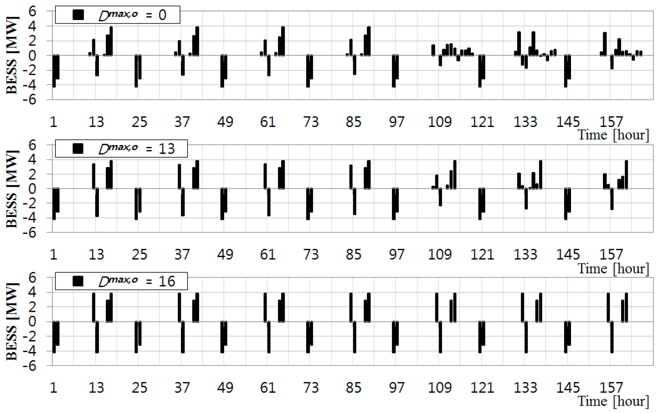
| Classification | Weekly Operation Mode | Daily Operation Mode | ||||
|---|---|---|---|---|---|---|
| Consideration of Historical Peak-value | No | Yes | Yes | No | Yes | Yes |
| Dmax,o (MW) | 0 | 13 | 16 | 0 | 13 | 16 |
| Used Energy of BESS (MWh) | 281.53 | 296.47 | 324.21 | 277.53 | 296.47 | 324.21 |
| Applied Peak wihout BESS (MW) | 15.15 | 15.15 | 16 | 15.15 | 15.15 | 16 |
| Applied Peak wih BESS (MW) | 11.98 | 13 | 16 | 11.98 | 13 | 16 |
| Reduction of Applied Peak (MW) | 3.17 | 2.15 | 0 | 3.17 | 2.15 | 0 |
| Demand Charge Savings (million KRW) | 23.39 | 15.89 | 0 | 23.39 | 15.89 | 0 |
| Energy Charge Savings (million KRW) | 25.94 | 29.38 | 31.12 | 24.56 | 29.38 | 31.12 |
| Total Savings (million KRW) | 49.34 | 45.27 | 31.12 | 47.94 | 45.27 | 31.12 |
| Savings Rate | 6.07% | 5.57% | 3.80% | 5.90% | 5.57% | 3.80% |
| Reduced Cycle-life (cycles) | 38.21 | 40.24 | 44.00 | 37.67 | 40.24 | 44.00 |
© 2017 by the authors. Licensee MDPI, Basel, Switzerland. This article is an open access article distributed under the terms and conditions of the Creative Commons Attribution (CC BY) license ( http://creativecommons.org/licenses/by/4.0/).
Share and Cite
Park, Y.-G.; Park, J.-B.; Kim, N.; Lee, K.Y. Linear Formulation for Short-Term Operational Scheduling of Energy Storage Systems in Power Grids. Energies 2017, 10, 207. https://doi.org/10.3390/en10020207
Park Y-G, Park J-B, Kim N, Lee KY. Linear Formulation for Short-Term Operational Scheduling of Energy Storage Systems in Power Grids. Energies. 2017; 10(2):207. https://doi.org/10.3390/en10020207
Chicago/Turabian StylePark, Yong-Gi, Jong-Bae Park, Namsu Kim, and Kwang Y. Lee. 2017. "Linear Formulation for Short-Term Operational Scheduling of Energy Storage Systems in Power Grids" Energies 10, no. 2: 207. https://doi.org/10.3390/en10020207