Article

Hydrothermal Carbonization of Waste Biomass: Process Design, Modeling, Energy Efficiency and Cost Analysis

Department of Civil, Environmental and Mechanical Engineering, University of Trento, Via Mesiano 77, 38123 Trento, Italy
*
Author to whom correspondence should be addressed.
Energies 2017, 10(2), 211; https://doi.org/10.3390/en10020211
Submission received: 23 December 2016 / Revised: 27 January 2017 / Accepted: 4 February 2017 / Published: 13 February 2017
(This article belongs to the Special Issue Thermo-Chemical Conversion of Waste Biomass)

Abstract

:
In this paper, a hydrothermal carbonization (HTC) process is designed and modeled on the basis of experimental data previously obtained for two representative organic waste materials: off-specification compost and grape marc. The process accounts for all the steps and equipment necessary to convert raw moist biomass into dry and pelletized hydrochar. By means of mass and thermal balances and based on common equations specific to the various equipment, thermal energy and power consumption were calculated at variable process conditions: HTC reactor temperature T: 180, 220, 250 °C; reaction time θ: 1, 3, 8 h. When operating the HTC plant with grape marc (65% moisture content) at optimized process conditions (T = 220 °C; θ = 1 h; dry biomass to water ratio = 0.19), thermal energy and power consumption were equal to 1170 kWh and 160 kWh per ton of hydrochar produced, respectively. Correspondingly, plant efficiency was 78%. In addition, the techno-economical aspects of the HTC process were analyzed in detail, considering both investment and production costs. The production cost of pelletized hydrochar and its break-even point were determined to be 157 €/ton and 200 €/ton, respectively. Such values make the use of hydrochar as a CO2 neutral biofuel attractive.

1. Introduction

Hydrothermal carbonization (HTC) is an induced coalification process that converts raw biomass into a coal-like product, called hydrochar, characterized by high carbon content and high calorific value. This type of thermo-chemical conversion, also referred to as wet pyrolysis (or wet torrefaction), can be applied to a variety of non-traditional sources such as the organic fraction of municipal solid waste, wet agricultural residues, sewage sludge, algae and aquaculture residues [1,2,3,4]. Indeed, unlike traditional dry pyrolysis [5,6], the HTC process allows for the treatment of substrates with elevated moisture content, up to 75%–90%, without requiring a drying pre-treatment step [4].
The HTC process is performed in high-pressure vessels by applying relatively high temperature (generally in the range 180–250 °C) and pressure (approximately 10–50 bar) to biomass in liquid water for a few hours (0.5–8 h) in the absence of air.
During HTC, the biomass undergoes dehydration, decarboxylation and decarbonylation reactions: the biomass is converted into a carbon-densified product, hydrochar, which can be used for many applications. Hydrochar can be used as fuel [7,8] in existing coal-handling infrastructure and it is therefore very attractive for co-firing [9]. Hydrochar was proposed as a feedstock for supercritical water gasification in a scenario where small HTC plants, placed in the production location of the residual biomass, feed a centralized high-tech gasification unit by hydrochar [10]. Hydrochar can be used as soil amendment to improve soil nutrient retention capacity by increasing the nutrient supply for plants and decreasing losses due to leaching [4]. Hydrochar shows potential for added-value applications in the field of advanced materials as an adsorbent and raw material for activated carbon production [11,12], hydrogen storage, electrochemical energy storage with lithium-ion batteries or super-capacitors [4,13].
For these reasons, HTC has recently attracted considerable interest in the research field. While a substantial amount of lab-scale experimental research on HTC reactions has been published, assessments of potential technical performance of industrial-scale HTC facilities are absent from the scientific literature. Though some pilot-scale HTC plants have been constructed in recent years [14], to date the detailed structure of such plants and their efficiency are still unknown to the vast majority of those involved in the HTC research field. Moreover, only a few authors have analyzed the energy efficiency of HTC plants by means of a modeling approach [15,16]. Prior studies document mass and energy balances of the HTC plant, but refer to a single HTC process condition. Stemann et al. [15,16] selected one mid-range HTC temperature (220 °C [15] and 210 °C [16]) and one residence time (4 h), using a biomass to water ratio of 0.2 and 0.14, respectively, without accounting for the variation of energy efficiency with processing conditions. Stemann et al.’s work [15,16] provides useful reference data, though it is not wide enough to enable HTC process optimization.
Thus, considering the emerging interest in the HTC process and the current state of the art, and to allow the technology to make a step forward from research to innovation, it is necessary to provide an in-depth analysis of the energy balance of the process. This will allow for determination of its energy sustainability. To bring the technology to market, a further step is necessary: an analysis intended to evaluate the economic feasibility of the HTC process and its profitability. These are the main objectives of the present study, which reports detailed energy and cost analyses of a proposed HTC plant layout.
Thus, first a process for an industrial-scale HTC continuous plant is designed. Then, its energy performances are evaluated considering several different HTC process conditions (reaction temperature T: 180 °C, 220 °C, 250 °C; reaction time θ: 1 h, 3 h, 8 h) and two different substrates with significantly different moisture content. Thermal and electric energy specific consumption and plant energy efficiencies are calculated for the various cases analyzed. To achieve these goals, an accurate process model was developed which estimates the mass and energy balances of all the equipment present in the path to transform raw biomass to dry pelletized hydrochar for sale. The modeling assumptions regarding HTC yields and product compositions were based on laboratory data of experimental runs performed on two types of biomass representative of organic waste: off-specification compost and grape marc.
Finally, the analysis moves to the evaluation of HTC investment and process costs. Specific costs and the hydrochar break-even value related to the HTC plant at its best performance process conditions are calculated. The HTC process, run in the proper operating conditions, is indeed of interest not only from an environmental point of view (circular economy and zero-waste approaches) but also from an economic standpoint.

2. Methods

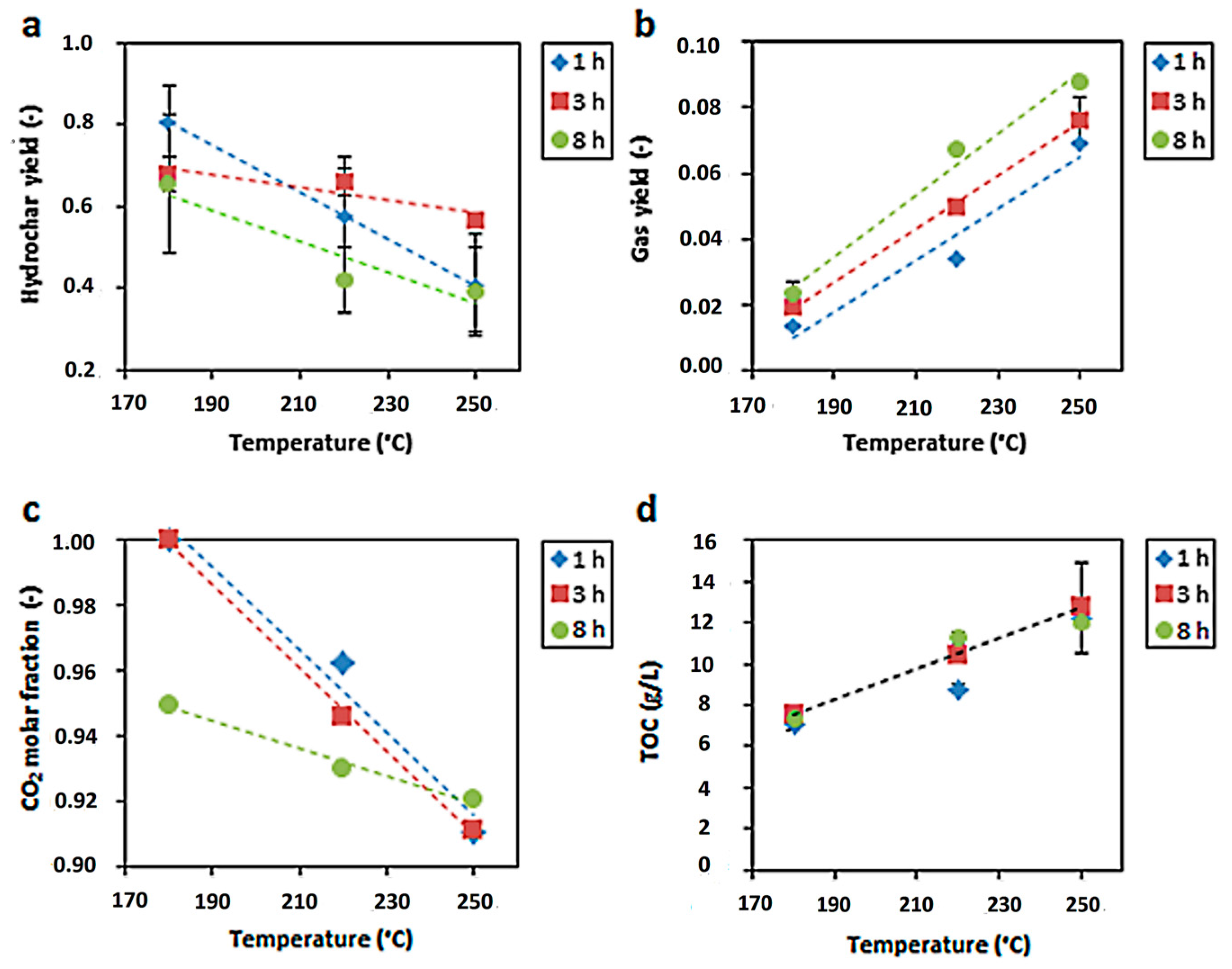
2.1. Experimental Data and Their Interpolation

The process model, developed to simulate a continuous HTC plant with all the auxiliary equipment (see Section 2.2), uses HTC experimental data previously obtained by our research group [17,18]. Experiments were performed in a stainless steel batch reactor, with an internal volume of 50 mL. Scale-up experiments performed by Hoekman et al. [19] demonstrate that HTC experimental results obtained in batch reactors are representative of those obtained when operating in continuous mode at a different reactor scale.
The types of feedstock used in the experiments were “off-specification compost” (OSC), coded by the European Waste Catalogue as EWC 19.05.03 [17], and grape marc (GM) [18]. OSC is a bio-stabilized material that is discarded and landfilled following the composting process because of its large particle size (between 10 and 40 mm). GM is a by-product of the wine industry. GM could be seen as a secondary raw material for innovative food applications [20]. Although it is often used for the production of spirits through distillation, it is still found as lignocellulosic residue at the end of this process (exhausted GM). Our experimental measures revealed moisture content of about 30% for OSC [17] and 65% for GM [21].
For both feedstocks, model simulations were performed at three residence (reaction) times (θ = 1, 3 and 8 h) and three reaction temperatures (T = 180, 220, 250 °C), maintaining a dry biomass to water ratio (DB/W) equal to 0.07 for OSC and 0.19 for GM: exactly the same conditions as in the experimental tests.
For modeling, the feedstock and hydrochar compositions were identified by their ultimate analysis. As a procedural hypothesis, both biomasses were considered to be only composed of carbon, hydrogen, oxygen, and ashes. Nitrogen and sulphur, present in small to negligible amounts, were considered to be part of the ashes.
In order to perform the mass balances of the HTC process, yields in solid, gas, and liquid phases were required—with yield being defined as mass of the phase produced per mass of dry feedstock. Experimental data shows that temperature affects hydrochar and gas yields more strongly than residence time. Moreover, experimental data reveals a linear dependence of yields with temperature. Thus, the yield values obtained experimentally for each combination of residence time and temperature were correlated using linear regression, as expressed by Equation (1):
Y = a x + b
where “Y” is solid (or gas) yield, and “x” is temperature (°C). Coefficients “a” and “b”, depending on residence time, are given in the Supplementary Materials (Table S1) for both solid and gaseous products and both biomasses. Correlations for OSC are depicted in Figure 1a,b. The liquid yield, due to liquid species derived from feedstock decomposition during HTC, was calculated by difference (liquid yield = 1 − solid yield − gas yield).
The gaseous products were modeled as CO2, CO, H2, and CH4, in line with gas-chromatographic analytical data. To quantify the amount of each species present in the gas, the regression curves between molar fractions and temperature were estimated. The procedure used was the same as that for gas and solid yields, where “Y” is, in this case, the molar fraction of each gas species. The regression curve between molar fraction of CO2 and temperature is shown in Figure 1c for OSC, while the values of “a” and “b” for both feedstocks and all the gaseous species are given in the Supplementary Materials (Table S1).
The liquid produced during HTC consists of several organic and inorganic compounds initially present within the feedstock. No detailed compositional data regarding the liquid phase from HTC of OSC and GM is available in the literature. That said, phenol was chosen as the species representative of the whole organic liquid mixture, and it was utilized to compute the mass balances of the various elements. This assumption is based on the work by Xiao et al. [22], who measured the composition of the liquid deriving from HTC of maize stalk and Tamarix ramosissima, ligno-cellulosic feedstocks such as OSC and GM. Results show that the liquid was mainly composed of phenols (lignin-derived species) with different substitution patterns. Surely, considering the liquid phase as consisting of only water and phenol is a very basic simplification; nevertheless, it is a procedural hypothesis which enables one to write the C, H, and O elemental mass balances and has no practical implications on the calculation of the process energy duties, one of the main goals of this work.
The total organic content (TOC) of the liquid phase from HTC was used to compute the amount of phenol as the representative species of the organic liquids. HTC lab tests performed on OSC [17] show that TOC values increase at increasing temperature: Figure 1d. Time plays a marginal role, such that only temperature dependence was taken into account. The trendline can be expressed as Equation (1), where “a”, “b”, and R2 are equal to 0.0721, −5.6959, and 0.9157, respectively. As far as GM is concerned, TOC values did not exhibit an evident trend with process conditions: thus, a mean value equal to 14.85 g/L was considered for each combination of residence time and temperature. The amount of phenol (C6H6O) was calculated by considering the carbon balance: each mole of phenol corresponds to 1/6 moles of carbon determined by multiplying the value of TOC and the volumetric flow rate of liquid inside the reactor.
The developed model does not take into account the inorganic elements present in the liquid phase; considering the mass balances of such inorganic species was beyond the scope of the present work. The amount of water present in the liquid phase results from the water added to the feedstock before feeding it to the HTC reactor, and the water produced during HTC. The water produced during HTC was calculated as the difference between liquid yield and the amount of phenol produced per mass of dry feedstock. The production of water during biomass hydrothermal processing was previously documented in the literature [23].

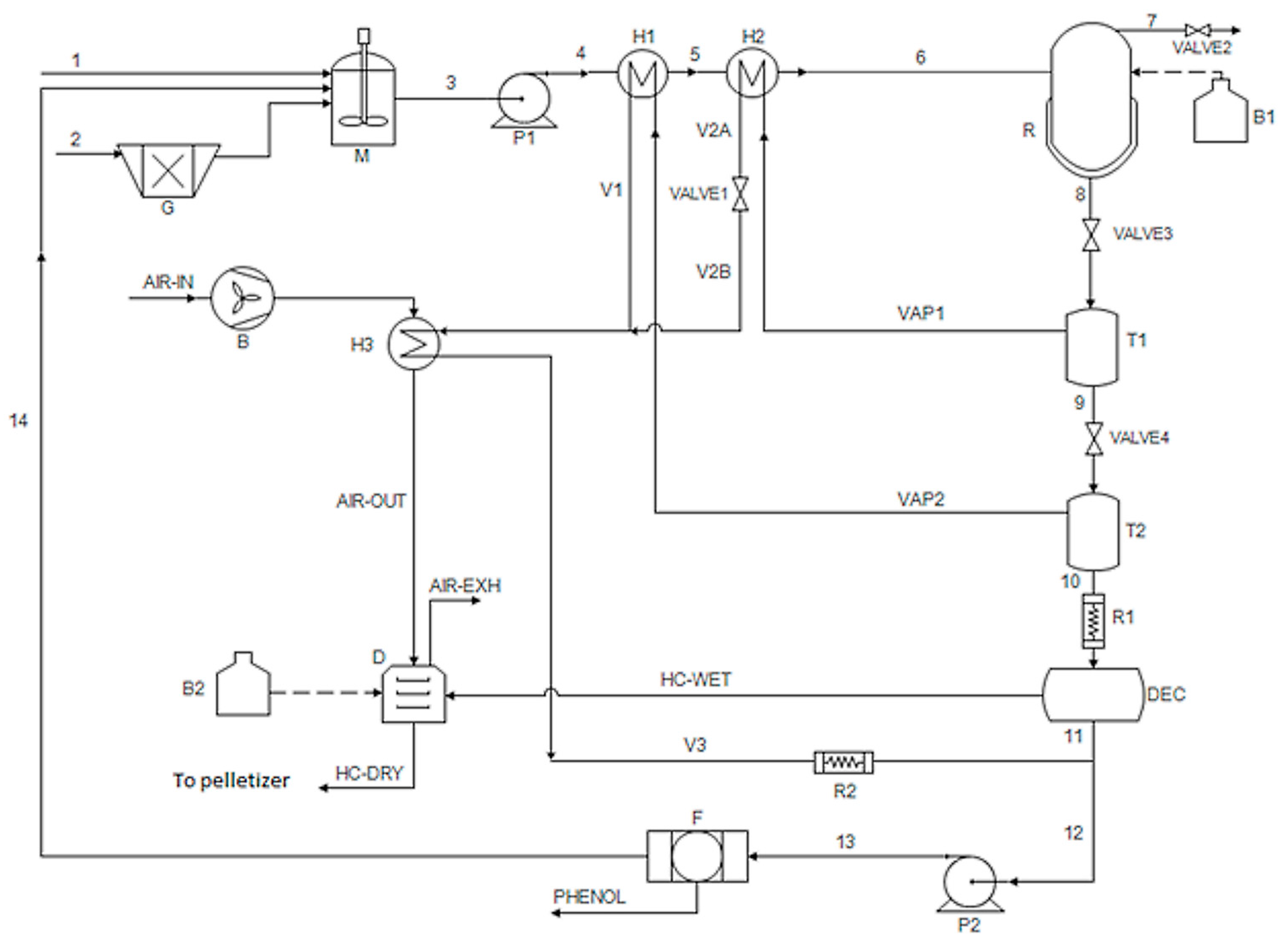
2.2. Conceptual Process Design

Figure 2 shows the conceptual process design developed for an industrial-scale HTC plant. The biomass (stream 2) is firstly processed in a grinder (G), which reduces and homogenizes its particle size. The feedstock is then mixed with water (stream 1) to reach the expected DB/W. Downstream the mixer (M), a pump (P1) and two heat exchangers in series (H1 and H2) are present.
The pump raises pressure to feed the slurry to the HTC continuous reactor. The heat exchangers preheat the biomass slurry. Next, the mixture (stream 6) enters the top of the reactor (R), while the HTC slurry, containing hydrochar and aqueous products, is removed from the bottom (stream 8). Gases formed during the reactions escape from the upper part of the reactor, passing through a valve (VALVE2) that, together with VALVE3, regulates pressure inside the reactor. The methane burner (B1) raises the temperature of the preheated biomass slurry up to HTC temperature (180–250 °C). The HTC slurry is then depressurized in two stages in flash tanks T1 and T2. The slurry exiting T2 is conveyed to a decanter (DEC), where liquid-solid separation is performed. The solid, i.e., hydrochar (stream HC-WET), is then transferred to an air-dryer (D), fed by an air blower (B), and heated by methane burner B2. After drying, the hydrochar produced is transferred to a pelletizer. Vapors produced by the expansion of the liquid slurry (streams VAP1 and VAP2) are used to preheat the biomass slurry in H1 and H2 and the air (stream AIR-IN) to the drier in heat exchanger H3. The condensed vapor (stream V3), together with the liquid exiting the decanter (stream 11), is pumped (P2) in order to be recycled to the process. Filter F separates organic liquids (phenol in the current simplification) from process water, which is recirculated to mixer M. The presence of filter F is not mandatory: the liquid from the decanter (DEC) could be recycled to the process—totally or partially—which could be beneficial in terms of increasing hydrochar yields [15,16]. Vice versa, if the HTC process aqueous phase is recovered for other applications, for instance as a liquid fertilizer, the use of the filter becomes an obvious choice. In this case, the separation of phenol-like compounds from the liquid is required because phenols are toxic species for plants. Considering the above, to be conservative, we considered the presence of the filter F (activated carbon filter) in the HTC process scheme, and its pressure drop was estimated to be 1.5 bar.

2.3. Process Model and Simulations

This section presents the modeling assumptions related to the process. The Appendix A reports details concerning the various pieces of equipment involved in the process (Figure 2) and the relevant key formulas. Based on such process assumptions and equipment formulas, it was possible to perform the calculations regarding mass balances, thermal duty, and power demand for the various pieces of equipment in the process.
The process model was self-developed using the programming language C#. The software code presents a friendly, easy-to-operate user-interface: some examples of the user-interface are given in the Supplementary Materials (Figure S1).
The plant was designed to have an operating time of 8000 h/y and a treatment capacity of 20,000 ton/y (2500 kg/h) of biomass as such or “as received”. Each piece of equipment was assumed to be stationary and adiabatic. Heat losses were simplified as to be occurring in two heat exchangers (R1 and R2) specially inserted in the scheme: Figure 2. Furthermore, no material losses were considered to take place during processing. Pressure drops were considered concentrated in the equipment.
Table 1 summarizes the values of flows entering the plant.

2.4. Efficiency Parameters: Thermal Efficiency and Plant Efficiency

A good estimation of the plant thermal efficiency is provided by the ratio between the thermal energy contained in the hydrochar produced and the thermal energy used to produce it given by the following equation:
T h e r m a l   e f f i c i e n c y =   E n e r g y H C , H H V E n e r g y t h
More precisely, thermal efficiency was computed as the ratio between the HHV of the produced dried hydrochar (i.e., hydrochar exiting the dryer with a residual 8% moisture content, see Appendix A)—expressed in kWh/kghydrochar—and the overall thermal energy required by the plant—expressed in kWh/kghydrochar. Hydrochar HHV was computed by referring to linear correlations between hydrochar yield and HHV extrapolated from the experimental data previously obtained by our research group [17,18]. Such HHV data refers to dry hydrochar, and was duly modified to take into account its residual 8% moisture content. The plant’s overall efficiency based on HHV was estimated through Equation (3), as proposed by Stemann and Ziegler [16]:
P l a n t   e f f i c i e n c y = E n e r g y H C , H H V E n e r g y b i o m a s s , H H V + E n e r g y e + E n e r g y t h
Differently form Equations (2), Equation (3) contains in the denominator the energy content of the raw moist feedstock (expressed in terms of its HHV) and the electric energy consumed by the plant. Notably, the two biomasses present very different HHVs owing to their significantly different moisture content (HHV = 11.74 MJ/kg for OSC with 30% moisture content; HHV = 6.78 MJ/kg for GM with 65% moisture content). The plant efficiency was assessed both not considering (to be conservative) and considering the heat of the slightly exothermic HTC reaction, as detailed in Appendix A.5 Reactor in the Appendix A.

3. Results and Discussion

This section presents the results of the process model simulations. Particular attention is given to electric and thermal energy consumption.

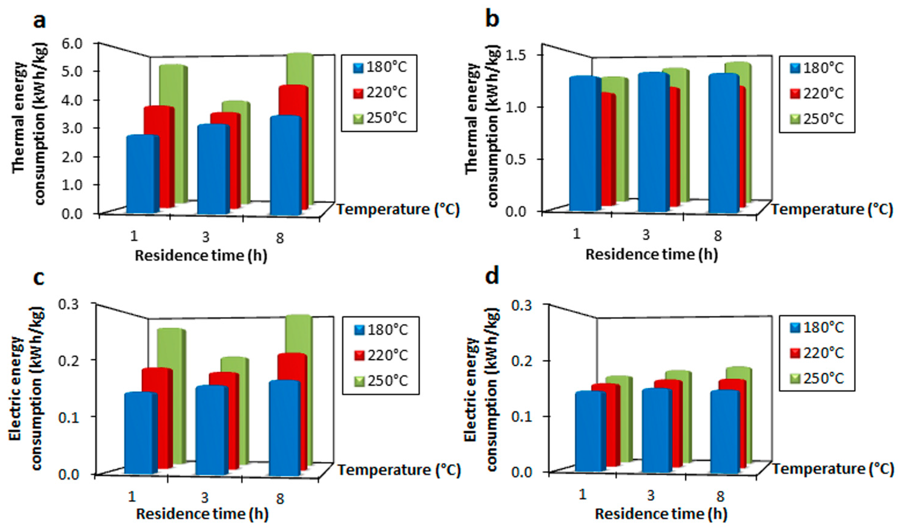
3.1. Electric Energy Consumption

In the proposed layout, the following equipment requires electric energy: the grinder, the mixer, pumps P1 and P2, the decanter, the air blower and, finally, the pelletizer. As reported in Table 2, the greatest consumption is recorded for the pelletizer and the piston pump.
The pelletizer requires up to 38.3% (both for OSC and GM) of total electricity demand. The pelletizer consumption depends on the hydrochar flow rate it has to treat, which varies with HTC residence time and temperature. Interestingly, in case of OSC, at 220 °C and 250 °C the electricity demand of the pelletizer reaches its maximum for a residence time of 3 h. As shown in Figure 1, at 220 °C and 250 °C a residence time of 3 h assures the highest hydrochar yields. This is not the case for GM, where the hydrochar yield [18] and consequently the pelletizer consumption are maximized for a residence time of 1 h. Electricity demand for the piston pump is in the range 19.6%–45.8% (OSC) and 8.8%–20.3% (GM) of total electricity demand. Percentages increase with HTC reaction temperature: the higher this temperature, the higher is reactor pressure and thus the power needed by pump P1. The grinding power demand, equal to 25.60 kW and 23.91 kW for OSC and GM, respectively, does not depend on process conditions. The grinder’s power demand is in the range 11.5%–14.0% (OSC) and 24.2%–25.9% (GM) of total power demand.
The air blower requires 7.1%–14.7% (OSC) and 11.0%–14.8% (GM) of total power demand. The blower power demand is maximum at the lowest HTC temperature and reaction time (i.e., 180 °C and 1 h) and minimum at the highest HTC temperature and reaction time (i.e., 250 °C and 8 h). This follows from the dependence of hydrochar yield on HTC process conditions.
With regards to the other contributions, the mixer and pump P2 power consumption is relatively low with respect to that of other components, and the decanter power demand varies marginally, decreasing with temperature. This is due to the dependence of the decanter power on the mass flow rate processed in the equipment. At higher HTC temperatures, higher vapor fluxes exit flash tanks T1 and T2 and, consequently, a lower amount of liquid slurry requires liquid-solid separation. Data reported in Table 2 (except for air blower and pelletizer) is influenced to a negligible extent or not at all by the residence time in the reactor.

3.2. Thermal Energy Consumption

In the modeled HTC plant, thermal power is required both to heat biomass slurry up to HTC reaction temperature and to dry hydrochar. Table 3 reports the consumption patterns of burners B1 and B2.
When OSC is considered, most of the thermal energy is used by B1, which requires between 81.1% and 91.7% of the total thermal energy demand. As for GM, the consumption patterns of B1 and B2 are much more similar. In general, as it should be expected, the lower the HTC temperature, the lower is the thermal energy required by B1. When using GM, B1 thermal power is slightly lower at 220 °C than at 180 °C: this is due to a counter-balancing effect of a much lower thermal flux available to pre-heat the biomass slurry in H2 when operating the reactor at 180 °C. Conversely, the lower the HTC temperature, the higher are the thermal energy requirements of B2. At lower HTC temperature, the amount of hydrochar produced is higher and, consequently, a greater amount of water has to be evaporated in the dryer, hence increasing B2 energy demand. Moreover, lower HTC temperature leads to lower evaporation of liquid in flash tanks T1 and T2, and a lower flow rate is available to preheat the air entering heat exchanger H3, which further increases B2 requirements.

3.3. Specific Energy Consumption

The values of the specific thermal energy consumption (kWh/kghydrochar) are depicted in Figure 3a,b. They range between 2.79–6.28 kWh/kghydrochar for OSC and 1.17–1.50 kWh/kghydrochar for GM. For OSC, values increase with temperature for each residence time, maintaining an opposite trend with respect to the hydrochar yield. No trend is evident for GM. In this case, the lowest thermal energy requirement is recorded at 220 °C HTC temperature, where the difference between the pre-heating temperature of stream 6 and the reactor temperature is lower compared to the other two cases (ΔT = 81 °C for 220 °C, ΔT = 88 °C for 180 °C and ΔT = 95 °C for 250 °C). When considering thermal energy consumption per unit of the biomass treated, values are in the range 1.65–1.85 kWh/kgfeedstock for OSC and 0.30–0.38 kWh/kgfeedstock for GM.
The specific electric energy consumption is low and does not exceed 0.30 kWh/kghydrochar for both types of biomass: Figure 3c,d.

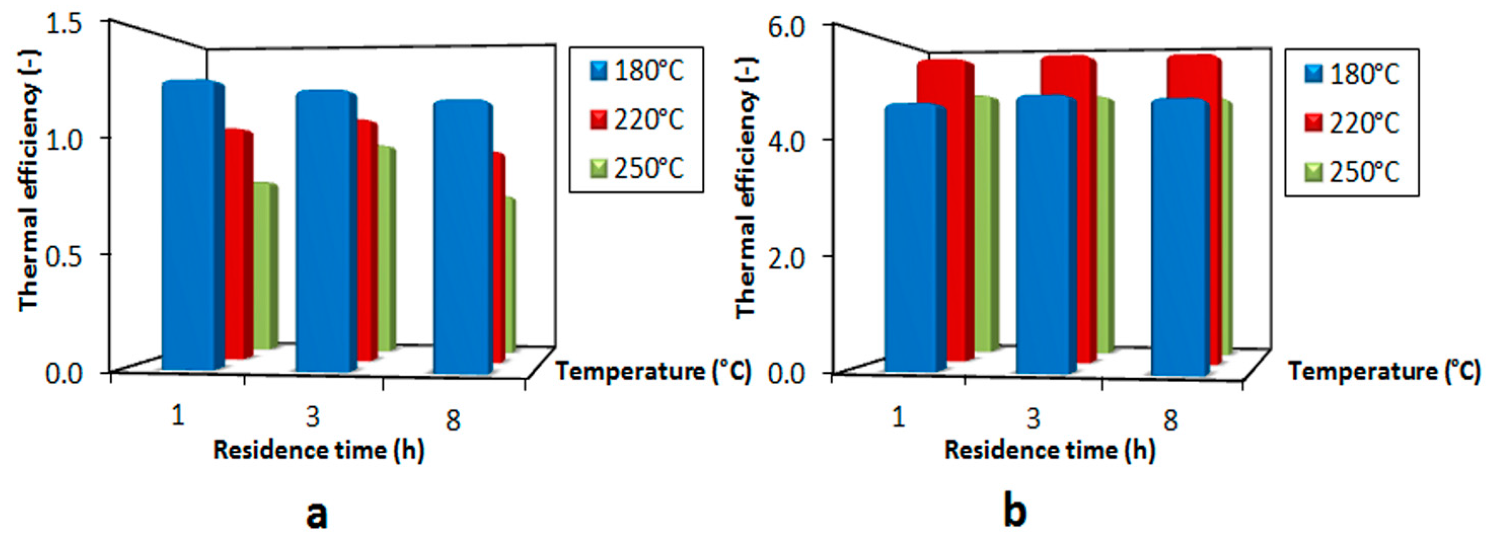
3.4. Thermal Efficiency

Figure 4 shows the thermal efficiency values, which are of interest when considering the use of hydrochar as fuel. Values are lower when using OSC with respect to GM: this is mainly due to the different DB/W ratio used for the two feedstocks (DB/W = 0.07 for OSC and DB/W = 0.19 for GM). A much greater amount of water per unit mass of dry feedstock is processed in the case of OSC in respect to GM. For OSC, thermal efficiency is only above one for all the residence times considered when the HTC temperature equals 180 °C. At higher temperatures, the energy content of OSC-derived hydrochar cannot provide sufficient thermal energy to compensate for the thermal requirements of the HTC process. Conversely, thermal efficiency for GM ranges between 4.67 and 5.64: the relatively high DB/W chosen (=0.19) allows for significantly improved HTC thermal performance, since a limited amount of water has to be processed per mass unit of feedstock. As mentioned in Section 2.3, plant thermal energy losses are simplified as being concentrated in heat exchangers R1 and R2. As an indicative value for all the process conditions and valid for both biomasses, thermal losses in R1 and R2 account for about 40% of the total heat demand reported in Table 3.

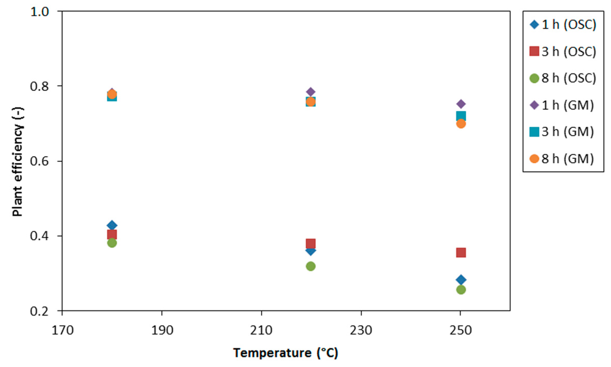
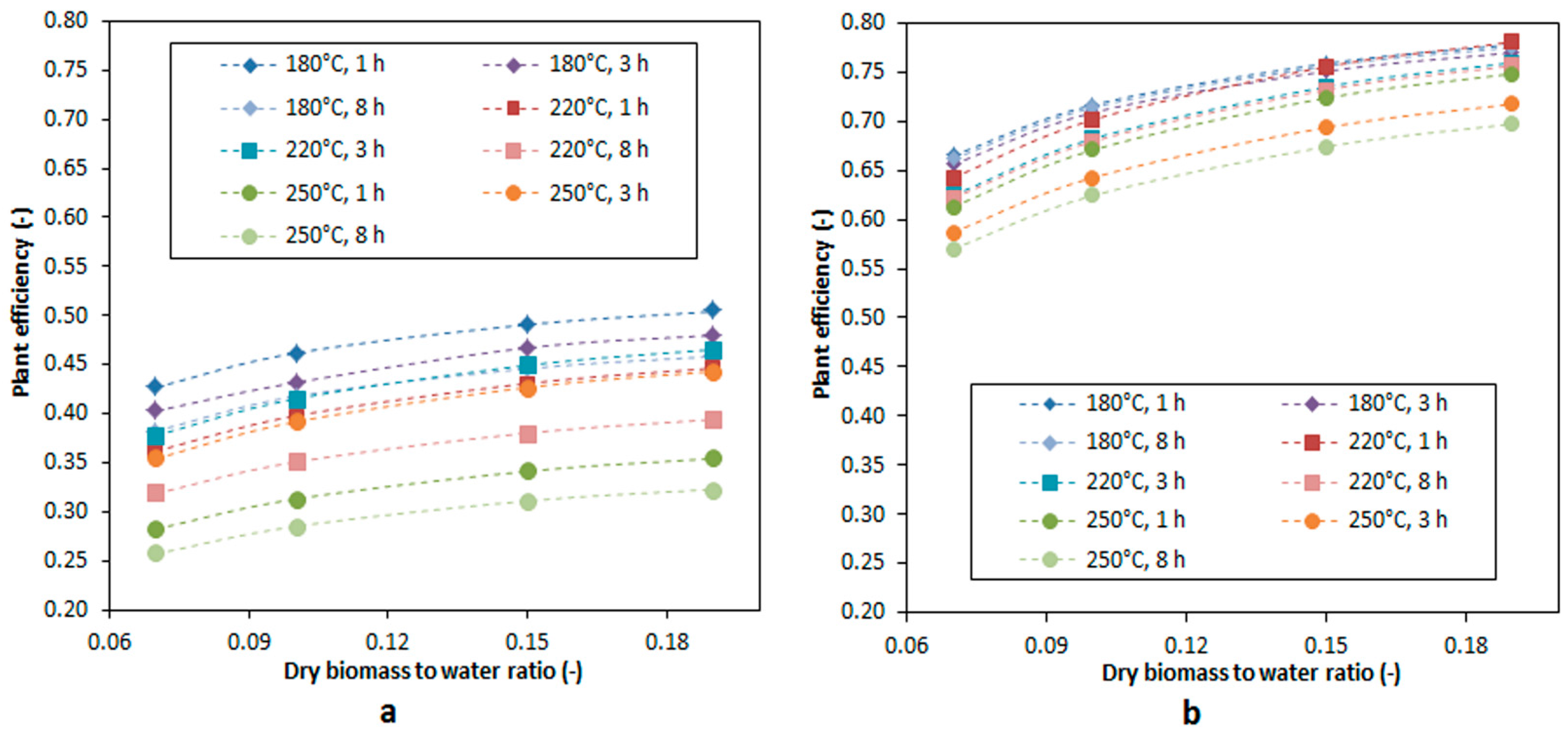
3.5. Plant Efficiency

Figure 5 shows the overall plant efficiency for both feedstocks. Results show a decreasing trend with temperature, even though in the case of GM the plant efficiency is practically equivalent for 180 and 220 °C. When using GM, plant efficiency values are notably higher than for OSC. Such differences are due to two factors. Firstly, the two raw substrates show significantly different moisture contents, which translates into significantly different HHVs. Secondly, the much lower DB/W in case of OSC hinders the process performance, as already pointed out when discussing thermal efficiency.
When accounting for HTC reaction heat (see Appendix A, Appendix A.5 Reactor), plant efficiency increases by about 1%–2%. Considering the great impact of DB/W on efficiency, the process model was run varying this parameter in the range 0.07–0.19 for both substrates. As a simplifying assumption, solid, liquid and gas yields were supposed not to depend on DB/W. The parameter that should be most affected by DB/W is the TOC of the HTC liquid. The higher the DB/W, the higher the TOC should be, i.e., the higher the phenol and organic acids concentration in the aqueous stream. For simplicity, such dependence was ignored here, the focus being on energy efficiency, which is influenced by liquid composition to a very negligible extent. The results of such analysis are depicted in Figure 6.
As expected, an increase in DB/W leads to higher plant efficiency in the case of OSC. In absolute terms, efficiency increases by 6.6%–8.5% when DB/W goes from 0.07 (experimental value) to 0.19 for all process conditions. As for GM, efficiency decreases by 11.2%–13.8% in absolute terms when DB/W goes from 0.19 (experimental value) to 0.07. In any case, in the whole range of DB/W investigated, plant efficiency is higher for HTC of GM with respect to HTC of OSC.

3.6. Economic Feasibility

For the purposes of economic evaluation, a HTC plant treating GM was considered. The plant operating conditions are those assuring the best results in terms of plant efficiency (T = 220 °C; θ = 1 h; DB/W = 0.19). At these operating conditions, the HTC reactor volume equals 8 m3 (height = 3 m; diameter = 1.84 m) taking into account the plant throughput (Table 1), the density of the slurry mixture which is equal to 920 kg/m3 (see Appendix A, Appendix A.2 Agitator), and the degree of filling of the reactor which was fixed at 75%. The reactor design pressure was fixed at 50 bar taking into account the vapor pressure of water at 220 °C (about 23 bar), a conservative overpressure of 10 bar due gas formation, and a safety factor of 1.5. All the equipment considered (including the reactor) are made of stainless steel. The plant configuration accounts for liquid recirculation from the decanter to the mixer (Figure 2).

3.6.1. Investment Costs

Table 4 reports the bare-module equipment costs, which include costs for the purchase of each process unit, their installation, transportation to the plant site and associated insurance expenses and taxes. All these costs were estimated according to the procedure indicated by Seider [24]. The price in dollars (year 2000) was converted in euros (1 US dollar = 0.87 euro) and actualized at year 2015 according to CEPCI 2015 [25]. In addition to equipment costs, capital costs are incurred for site preparation and for allocated costs to purchase the utility plants, as well as to cover contingencies and the contractor’s fee. The costs of land, start-up and working capital were added to the previous costs. In this way, the total capital investment cost (CTCI) was estimated: Table 5. In the case study, a considerable amount of waste water (1157 kg/h or equivalently 9263 t/y) results from the HTC process and the cost for its treatment has to be considered. The excess water produced is disposed of in a waste water treatment plant. The related cost was included in the operating costs in Section 3.6.2. The estimation of capital costs also factored in an activated carbon filter for organic acids and pollutants (phenol) removal from the recirculating aqueous stream.

3.6.2. Total Production Costs

With regards to operating costs, the cost of utilities for providing thermal energy and electric power were considered. The cost of methane was fixed at 0.3537 €/m3, while a mean cost value of 0.1066 €/kWh was assumed for electricity (both prices take into account the size of utility consumption and are referred to a factory located in Italy [26,27]). The number of plant operators was estimated to be equal to four, one operator per shift, as suggested by Seider [24] for a continuous plant with similar capacity treating fluid mixtures. For maintenance and spares, an annual cost equivalent to 8% of total depreciable capital CTDC was considered, i.e., 121,003 €. Finally, total annual production costs include property taxes and insurance (1% CTDC) and general expenses for product sales, research, administrative and management incentive compensation. The cost of water treatment was assumed to be equal to 13.7 €/ton, according to local legislation in Trentino (Italy) [28]. Overall operating costs are summarized in Table 6. The total production cost amounts up to 157 € per ton of hydrochar produced.

3.6.3. Cost Linked to the Capital and Selling Price of HTC Coal

Considering an average loan interest rate of 5% per year in the European Union [29] and assuming a repayment time of 10 years for the plant, an annual cost of 229,717 € is obtained for the repayment of the total capital investment (French amortization method). In order to assess the economic feasibility of the HTC plant, the minimum selling price of the product to make the plant economically viable was determined. Considering an annual production of 5317 tons of hydrochar (resulting from the simulation results at T = 220 °C and θ = 1 h) and the total annual cost (including total production costs and income taxes of 37%), the break-even value of hydrochar is equal to 200 €/ton. From an energy point of view, this value corresponds to 8.3 €/GJHHV (HHVhydrochar = 25.64 GJ/ton at T = 220 °C; θ = 1 h; DB/W = 0.19). This value is slightly lower than that obtained by Stemann et al. [15], who reported a value of €9.67/GJHHV for a HTC plant treating 40,000 tons/y of empty fruit bunches at similar process conditions (T = 220 °C; θ = 4 h; DB/W = 0.2). Considering the price of wood pellets, usually in the range 150–200 €/ton and depending on the country considered [30], the break-even value of hydrochar pellets (200 €/ton) makes hydrochar competitive with wood pellets. Interestingly, the value calculated here for hydrochar is comparable with the market price of hydrochar by Ingelia S.L., which is, to the best of our knowledge, the only company currently selling hydrochar (at a price of 150–200 €/ton [31]). Hydrochar’s competitive price and its better properties in terms of HHV and chemical composition compared to wood pellets encourage its usage as a fuel in biomass plants and district heating power stations. Conversely, it is evident that hydrochar cannot compete with coal, that is priced at 43 €/ton in 2016 [32]. However, the costs associated with CO2 emissions into the atmosphere, largely avoided when producing and using hydrochar, could favor the development of HTC plants and consequently of the hydrochar market, to complement or possibly replace coal.

4. Conclusions

A complete HTC process for converting moist biomass into pelletized dry hydrochar was designed and modeled. The process was simulated at various process conditions (T = 180, 220, 250 °C; θ = 1, 3, 8 h; DB/W in the range 0.07–0.19). The HTC plant was designed as capable to treat 20,000 ton/y of organic waste: grape marc with 65% moisture content, and off-specification compost with 30% moisture content.
Plant efficiency was found to be highly dependent on initial feedstock moisture content and DB/W: an increase in DB/W from 0.07 to 0.19 largely reduced energy consumption. In the most favorable conditions, i.e., when processing grape marc at DB/W = 0.19, T = 220 °C and θ = 1 h:
  • a plant efficiency of 78% was achieved;
  • specific thermal energy consumption was equal to 1.17 kWh/kghydrochar (0.31 kWh/kgfeedstock);
  • specific electric energy consumption was equal to 0.16 kWh/kghydrochar (0.04 kWh/kgfeedstock);
  • the production cost of pelletized hydrochar was equal to 157 €/tonhydrochar;
  • the hydrochar break-even value for a plant repayment period of 10 years was equal to 200 €/tonhydrochar, competitive with the price of wood pellets (150–200 €/tonwood).
The values calculated above are reference data to evaluate the techno-economic feasibility of HTC plants. Overall, the competitive price of pelletized hydrochar compared with pelletized wood seems promising and could encourage a large industrial-scale development of the HTC technology in the future.

Supplementary Materials

The following are available online at www.mdpi.com/1996-1073/10/2/211/s1, Table S1: Regression coefficients (a, b) and R-squared value (R2) of linear correlations—Equation (1) in the text—between temperature and solid yield, gas yield, molar percentage of gaseous products at different residence times (1, 3, 8 h) for OSC and GM, Figure S1: User-interfaces of the software code developed in C#.

Author Contributions

Michela Lucian conducted modeling and simulations and performed energy efficiency and costs analyses. Luca Fiori supervised the work and contributed to the discussions of the results. Both authors collaborated in designing the HTC process and writing the paper.

Conflicts of Interest

The authors declare no conflict of interest.

Appendix A

This appendix provides details on the equipment involved in HTC processing (Figure 2), together with the main representative equations used to calculate energy consumption.

Appendix A.1. Grinder

Particle size reduction of the feedstock allows for a larger surface area, increasing the reactivity of solids during further processing and simplifying the handling of materials. Among the different types of grinders, the hammer mill seems the most suitable for use with relatively soft fibrous-like materials such as OSC and GM. The specific power demand for milling depends on the feedstock, as well as the required particle sizes and the type of mill. Here, milling is simply characterized by its power demand based on data from literature. A realistic way of estimating power requirements for grinding was proposed by Bond [33]. If most of the feed—whose flow rate is m ˙ W B (ton/h)—passes through a mesh size of D p , i (mm) and the product passes through a mesh size of D p , e (mm), gross power W G (kW), which includes friction in the grinder, is given by Equation (A1):
W G = 0.3162   m ˙ W B W i ( 1 D p , e 1 D p , i )
In the grinder, the size of incoming biomass is reduced from a mean particle size of 40 mm (OSC) and 20 mm (GM) to a mean particle size of 0.8 mm. W i (kWh/ton of feed) stands for Work Index. Owing to the lack of data regarding W i for ligno-cellulosic materials such as OSC and GM, W i was set equal to 13 kWh/ton (the value for coal) for both substrates [33]. A mechanical efficiency of 0.40 was assumed, since a value in the range 0.25–0.60 is typical for such machines [33].

Appendix A.2. Agitator

To create a mixture than can easily be pumped, the feedstock exiting the hammer mill is mixed with water in the agitator. An anchor agitator was selected, suitable for slurries and relatively high viscous liquids. The power to drive the impeller (namely the shaft power) W M (kW) was calculated as:
W M = N P N M 3 D i 5 ρ S
The revolution speed N M was fixed at 70 rev/min, a typical value for anchor impellers, while N P , analogous to a friction factor, was correlated with Reynolds number (Re) through Equation (A3) extrapolated by experimental data of Furukawa et al. [34].
N P = 94.043 R e 0.599
The impeller diameter D i (m) was calculated through the mixer diameter D M (m) fixing a mixer volume of 3 m3 and using a ratio D i / D M equal to 0.892 as proposed by Furukawa et al. [34]. The slurry density ρ S was determined using the mixture rule and considering a dry biomass density equal to 500 kg/m3 for both OSC and GM. The apparent viscosity of the slurry was considered equal to 1 Pa·s. The motor’s power is higher than the power required for the impeller to compensate losses in gearbox, seals and bearings. A motor efficiency of 0.80 was assumed to calculate the power consumed.

Appendix A.3. Pumps

A piston pump was considered the most suitable for pumping the slurry to the reactor: piston pumps are also suitable for viscous fluids and streams involving particles, and can be used in a wide range of pressure conditions, up to 300 bar [35].
The pump has to ensure pressure to the reactor ( P R ) and compensate pressure drops in heat exchangers H1 and H2 ( Δ P H 1 and Δ P H 2 , conservatively assumed to be equal to 3 bar each). P R results from the water vapor pressure ( P s a t ) at reactor temperature, and the partial pressure of gaseous species produced within the reactor ( P g ). P s a t was calculated through Antoine’s equation [36], while P g was fixed at 10 bar − value considered constant in the reaction temperature range 180–250 °C. From a practical point of view, this means fixing the pressure set-point of control valve VALVE2 (and also VALVE3) to a value equal to P s a t + P g . Summing up, the discharge pressure ( P P ) of the piston pump follows from Equation (A4):
P P = P s a t + P g + Δ P H 1 + Δ P H 2
The pump motor power demand was calculated as the product of the slurry volumetric flow rate (m3/s) and pressure increment P P (bar), taking into account an overall pump efficiency of 0.50 [37]. The other pump of the plant, P2, is needed to provide liquid recirculation. A centrifugal type pump was selected in this case, since the rise in pressure required is modest (assumed equal to 2 bar), and the stream to be pumped does not contain solids. Power consumption was calculated in the same way as for the piston pump, fixing the centrifugal pump efficiency at a value of 0.40 [38].

Appendix A.4. Heat Exchangers

The slurry exiting the pump is preheated in two stages in counter-current flow heat exchangers H1 and H2. The maximum temperature value for the biomass exiting H2 was fixed equal to 155 °C, in order to avoid biomass decomposition that could cause fouling and clogging of the heat exchangers. This temperature was selected as hemicellulose decomposes at T > 180 °C, while most of the lignin and cellulose hydrolyze and decomposes at T > 200 °C [39,40].
The slurry flows through the tube-side of the heat exchangers. The sensible heat gained by the slurry is provided by the condensation latent heat of the vapors. Vapors enter the shell-side of the heat exchangers at saturated conditions and leave the equipment at condensation temperature without being further cooled. The specific heat of liquid water was expressed as a function of temperature using the polynomial correlations reported by Chilton [41]. The specific heat of both types of dry biomass was evaluated using the correlation for wood as proposed by Harada et al. [42], valid in the temperature range 25 °C–240 °C. The temperature of VAP2 was set equal to 120 °C—see below: “Flash separators”. The temperature of VAP1 was set dependent on reactor temperature, as detailed below in “Flash separators”. The maximum temperature of the slurry exiting H1 was fixed at 90 °C in order to maintain a minimum temperature difference of 30 °C with incoming vapors at 120 °C.

Appendix A.5. Reactor

After being pre-heated, the slurry enters the reactor where HTC takes place. A system of valves (VALVE2 and VALVE3) enables to keep pressure in the reactor constant. A diathermic oil jacket transfers the heat needed to raise the slurry temperature up to HTC temperature. For the reactor thermal balance, considering that HTC is slightly exothermic overall [16], two scenarios are possible. In the first scenario, the heat of reaction was conservatively set equal to zero. In the second scenario, the exothermal behavior of the reaction was taken into account. In this case, reaction heat was fixed equal to 500 J/g of dry biomass, a value experimentally measured by Stemann and Ziegler [16] for the HTC of poplar wood.
The thermal balance in the reactor accounts for the sensible heat increase of the slurry, the possible reaction heat, the sensible heat decrease of the diathermic oil, which enters the reactor jacket at 300 °C and exits at 265 °C. The specific heat of the diathermic oil was fixed equal to 2.5 kJ/kg °C [43].

Appendix A.6. Burners

A methane air burner provides the energy needed to heat the diathermic oil. Heat losses due to the release of hot flue gases generated by combustion in the burner were duly taken into account.
Combustion occurs assuming 30% excess air and the chimney temperature was set equal to 150 °C. Methane mass flow rate was determined considering its LHV (35.8 MJ/Nm3 [44]) and a burner efficiency of 90%. The same procedure was used when modeling burner B2, which provides the thermal power to raise the temperature of the air exiting heat exchanger H3 to 200 °C.

Appendix A.7. Flash Separators

The purpose of flash tanks T1 and T2 in series is to reduce the temperature of the slurry mixture exiting the reactor, and to vaporize a fraction of the liquid present in such stream. The vapor produced is then used to preheat the biomass slurry in H1 and H2.
In T1, the temperature of the slurry was supposed to drop to a temperature 50 °C lower than reactor temperature (TR – 50 °C), as a consequence of a controlled decrease in pressure. Conversely, T2 is operated at a pre-set pressure (about 2 bar) to guarantee that the vapor produced has enough pressure to flow through the rest of the plant (pressure drops in H1 and H3 assumed equal to 0.5 bar each).
T1 and T2 are adiabatic and operate at thermodynamic equilibrium. The liquid-vapor equilibrium was computed considering both phases composed by water and phenol, utilizing Raoult’s law and treating the liquid as an ideal mixture. The vapor pressure of both components was determined applying Antoine’s equation [36]. The thermal balance performed on the flash tanks enabled to calculate the flow rate of the various streams exiting T1 and T2.

Appendix A.8. Decanter

The aqueous stream and the hydrochar exiting flash tank T2 are conveyed to a centrifugal decanter (DEC) which separates liquid and solid fractions. It was assumed that the whole hydrochar exits the decanter as stream HC-WET, i.e., the solid separation efficiency is 100%. The hydrochar exits DEC with a residual moisture content of 50%, i.e., stream HC-WET consists of 50 wt. % (dry) hydrochar and 50 wt. % aqueous solution. Such moisture content is typical of mechanical dewatering systems applied to hydrochar. The remaining liquid exits the decanter as stream 11. The total power demand of the equipment ( W D ) was calculated as the sum of three single power demands [45], as reported in Equation (A5):
W D = W S + W L + W N L
where W S and W L are the power to convey hydrochar and liquid, respectively, in the decanter, while W N L is the no-load power which accounts for the friction losses in bearings, gearbox, and due to air friction on the decanter bowl. W S and W L were calculated as the product of the mass flow rate of solid and liquid and the power square of circumferential speed of solid and liquid at discharge ports. The circumferential speeds of liquid and solid were calculated multiplying the rotational speed of the bowl (s−1) by the discharge diameter (m) of solid and liquid, considered equal to 0.5 and 0.6 times the bowl diameter, respectively. The bowl speed depends on the bowl diameter. A diameter of 250 mm corresponds to 5000 rpm [45], and the rotational speed was therefore equal to 523 s−1. The no-load power was set equal to 0.5 times the sum of W S and W L , and the decanter motor efficiency was considered equal to 0.85.

Appendix A.9. Dryer and Air Blower

The hydrochar exiting the decanter is dried to reduce its liquid content from 50% to 8%, a value considered acceptable for hydrochar storage and usage as fuel. An adiabatic dryer in which the solids are exposed directly to hot air was selected.
The temperature of the air streams involved in drying was determined by using psychrometric charts, fixing an inlet (stream AIR-IN) and exit (stream AIR-EXH) air relative humidity of 70% and 80%, respectively, and an inlet and exit air temperature equal to 10 and 38 °C, respectively. Thus, the air enters at 10 °C, is pre-heated by heat exchanger H3, then burner B2 increases its temperature up to 200 °C, and finally, after the drying process, air is released at 38 °C.
The process model determines the air flow rate (as first attempt value) following psychrometric considerations. Then, the model checks if such value satisfies the thermal balance (i.e., if the heat released by air cooling from 200 to 38 °C is sufficient to heat the hydrochar and vaporize its moisture content). If the thermal balance is not respected, the model recalculates the air flow rate to achieve thermal balance.
A blower supplies the dryer with fresh air. The power of the blower W B (kW) was calculated with Equation (A6) [37]:
W B = 100 m ˙   Δ P B η B
where m ˙ is the air flow rate (m3/s) entering the blower, Δ P B is the increment in pressure (bar) provided by the equipment (fixed equal to 0.05 bar), and η B is its efficiency—assumed equal to 0.80 [37].

Appendix A.10. Pelletizer

The specific consumption of pelletizer was estimated equal to 51 kWh/tonhydrochar (same value as for wood), according to Obernberger and Thek [46].

References

  1. Afolabi, O.O.D.; Sohail, M.; Thomas, C.P.L. Microwave Hydrothermal Carbonization of Human Biowastes. Waste Biomass Valoriz. 2015, 6, 147–157. [Google Scholar] [CrossRef]
  2. Lu, X.; Berge, N.D. Influence of feedstock chemical composition on product formation and characteristics derived from the hydrothermal carbonization of mixed feedstocks. Bioresour. Technol. 2014, 166, 120–131. [Google Scholar] [CrossRef] [PubMed]
  3. Volpe, M.; Fiori, L.; Volpe, R.; Messineo, A. Upgrading of Olive Tree Trimmings Residue as Biofuel by Hydrothermal Carbonization and Torrefaction: A Comparative Study. Chem. Eng. Trans. 2016, 50, 13–18. [Google Scholar]
  4. Libra, J.A.; Ro, K.S.; Kammann, C.; Funke, A.; Berge, N.D.; Neubauer, Y.; Titirici, M.-M.; Fühner, C.; Bens, O.; Kern, J.; et al. Hydrothermal carbonization of biomass residuals: A comparative review of the chemistry, processes and applications of wet and dry pyrolysis. Biofuels 2011, 2, 71–106. [Google Scholar] [CrossRef]
  5. Volpe, R.; Messineo, A.; Millan, M.; Volpe, M.; Kandiyoti, R. Assessment of olive wastes as energy source: Pyrolysis, torrefaction and the key role of H loss in thermal breakdown. Energy 2015, 82, 119–127. [Google Scholar] [CrossRef]
  6. Volpe, M.; Panno, D.; Volpe, R.; Messineo, A. Upgrade of citrus waste as a biofuel via slow pyrolysis. J. Anal. Appl. Pyrolysis 2015, 115, 66–76. [Google Scholar] [CrossRef]
  7. Messineo, A.; Volpe, R.; Asdrubali, F. Evaluation of net energy obtainable from combustion of stabilised olive mill by-products. Energies 2012, 5, 1384–1397. [Google Scholar] [CrossRef]
  8. Gamgoum, R.; Dutta, A.; Santos, R.M.; Chiang, Y.W. Hydrothermal Conversion of Neutral Sulfite Semi-Chemical Red Liquor into Hydrochar. Energies 2016, 9, 1–18. [Google Scholar] [CrossRef]
  9. Kruse, A.; Funke, A.; Titirici, M.-M. Hydrothermal conversion of biomass to fuels and energetic materials. Curr. Opin. Chem. Biol. 2013, 17, 515–521. [Google Scholar] [CrossRef] [PubMed]
  10. Castello, D.; Kruse, A.; Fiori, L. Supercritical water gasification of hydrochar. Chem. Eng. Res. Des. 2014, 92, 1864–1875. [Google Scholar] [CrossRef]
  11. Titirici, M.-M. Sustainable Carbon Materials from Hydrothermal Processes, 1st ed.; John Wiley & Sons: West Sussex, UK, 2013. [Google Scholar]
  12. Wang, L.; Zhang, Z.; Qu, Y.; Guo, Y.; Wang, Z.; Wang, X. A novel route for preparation of high-performance porous carbons from hydrochars by KOH activation. Colloids Surf. A Physicochem. Eng. Asp. 2014, 447, 183–187. [Google Scholar] [CrossRef]
  13. Unur, E.; Brutti, S.; Panero, S.; Scrosati, B. Nanoporous carbons from hydrothermally treated biomass as anode materials for lithium ion batteries. Microporous Mesoporous Mater. 2013, 174, 25–33. [Google Scholar] [CrossRef]
  14. Hitzl, M.; Corma, A.; Pomares, F.; Renz, M. The hydrothermal carbonization (HTC) plant as a decentral biorefinery for wet biomass. Catal. Today 2015, 257, 154–159. [Google Scholar] [CrossRef]
  15. Stemann, J.; Erlach, B.; Ziegler, F. Hydrothermal carbonisation of empty palm oil fruit bunches: Laboratory trials, plant simulation, carbon avoidance, and economic feasibility. Waste Biomass Valoriz. 2013, 4, 441–454. [Google Scholar] [CrossRef]
  16. Stemann, J.; Ziegler, F. Assessment of the Energetic Efficiency of A Continuously Operating Plant for Hydrothermal Carbonisation of Biomass. In World Renewable Energy Congress, Linköping, Sweden, 8–13 May 2011; Linköping University Electronic Press: Linköping, Sweden, 2011; pp. 125–132. [Google Scholar]
  17. Basso, D.; Weiss-Hortala, E.; Patuzzi, F.; Castello, D.; Baratieri, M.; Fiori, L. Hydrothermal carbonization of off-specification compost: A byproduct of the organic municipal solid waste treatment. Bioresour. Technol. 2015, 182, 217–224. [Google Scholar] [CrossRef] [PubMed]
  18. Basso, D.; Patuzzi, F.; Castello, D.; Baratieri, M.; Rada, E.C.; Weiss-Hortala, E.; Fiori, L. Agro-industrial waste to solid biofuel through hydrothermal carbonization. Waste Manag. 2016, 47, 114–121. [Google Scholar] [CrossRef] [PubMed]
  19. Hoekman, S.K.; Broch, A.; Robbins, C.; Purcell, R.; Zielinska, B.; Felix, L. Process Development Unit (PDU) for Hydrothermal Carbonization (HTC) of Lignocellulosic Biomass. Waste Biomass Valoriz. 2014, 5, 669–678. [Google Scholar] [CrossRef]
  20. Lavelli, V.; Torri, L.; Zeppa, G.; Fiori, L.; Spigno, G. Recovery of Winemaking By-Products. Ital. J. Food Sci. 2016, 28, 542–564. [Google Scholar]
  21. Fiori, L.; Florio, L. Gasification and Combustion of Grape Marc: Comparison among Different Scenarios. Waste Biomass Valoriz. 2010, 1, 191–200. [Google Scholar] [CrossRef]
  22. Xiao, L.P.; Shi, Z.J.; Xu, F.; Sun, R.C. Hydrothermal carbonization of lignocellulosic biomass. Bioresour. Technol. 2012, 118, 619–623. [Google Scholar] [CrossRef] [PubMed]
  23. Castello, D.; Kruse, A.; Fiori, L. Biomass gasification in supercritical and subcritical water: The effect of the reactor material. Chem. Eng. J. 2013, 228, 535–544. [Google Scholar] [CrossRef]
  24. Seider, W.D.; Seader, J.D.; Lewin, D.R. Product and Process Design Principles: Synthesis, Analysis and Design, 2nd ed.; John Wiley & Sons: West Sussex, UK, 2004. [Google Scholar]
  25. CEPCI, 2015: Economic Indicators. Available online: http://www.chemengonline.com/economic-indicators-cepci/ (accessed on 15 May 2016).
  26. Autorità per L’energia Elettrica il Gas e il Sistema Idrico: Electrical Energy Prices. Available online: http://www.autorita.energia.it/it/dati/eepcfr2.htm (accessed on 16 May 2016).
  27. Autorità per L’energia Elettrica il Gas e il Sistema Idrico: Natural Gas Prices. Available online: http://www.autorita.energia.it/it/dati/gpcfr2.htm (accessed on 16 May 2016).
  28. Provincia Autonoma di Trento. Disciplinare Contenente le Prescrizioni per il Conferimento e Trattamento Presso gli Impianti di Depurazione di Proprietà della Provincia Autonoma di Trento dei Reflui di cui All’art. 95 Comma 5 del t.u.l.p. in Materia di Tutela Dell’ambiente Dagli Inquinamenti. Available online: http://www.appalti.provincia.tn.it/binary.php/pat_pi_bandi/bandi/X02_Allegato_A.1233076172.pdf (accessed on 23 December 2016).
  29. EU Commission, 2015: Access to Finance: Loans. Available online: http://ec.europa.eu/growth/access-to-finance/data-surveys/index_en.htm (accessed on 14 June 2016).
  30. European Biomass Industry Association: European Market. Available online: http://www.eubia.org/index.php/about-biomass/biomass-pelleting/economics-applications-and-standards (accessed on 1 May 2016).
  31. Ingelia Italia Srl. Available online: http://www.ingelia.it/ (accessed on 1 May 2016).
  32. Global Energy Statistics: Coal Prices. Available online: https://knoema.com/xfakeuc/coal-prices-long-term-forecast-to-2020-data-and-charts (accessed on 1 May 2016).
  33. McCabe, W.L.; Smith, J.C.; Harriott, P. Unit Operations of Chemical Engineering, 7th ed.; McGraw-Hill: New York, NY, USA, 2005. [Google Scholar]
  34. Furukawa, H.; Kato, Y.; Inoue, Y.; Kato, T.; Tada, Y.; Hashimoto, S. Correlation of Power Consumption for Several Kinds of Mixing Impellers. Int. J. Chem. Eng. 2012, 2012, 106496. [Google Scholar] [CrossRef]
  35. White, F. Fluid Mechanics, 7th ed.; McGraw-Hill: New York, NY, USA, 2011. [Google Scholar]
  36. NIST 2016. Antoine Equation Parameters. Available online: http://webbook.nist.gov/chemistry (accessed on 15 March 2016).
  37. Perry, R.H.; Green, D.W. Perry’s Chemical Engineers’ Handbook, 8th ed.; McGraw-Hill: New York, NY, USA, 2007. [Google Scholar]
  38. Sinnott, R.K. Chemical Engineering Design, 4th ed.; Coulson & Richardson: Oxford, UK, 2005. [Google Scholar]
  39. Yang, H.; Yan, R.; Chen, H.; Lee, D.H.; Zheng, C. Characteristics of hemicellulose, cellulose and lignin pyrolysis. Fuel 2007, 86, 1781–1788. [Google Scholar] [CrossRef]
  40. Poletto, M.; Zattera, A.J.; Forte, M.M.C.; Santana, R.M.C. Thermal decomposition of wood: Influence of wood components and cellulose crystallite size. Bioresour. Technol. 2012, 109, 148–153. [Google Scholar] [CrossRef] [PubMed]
  41. Coker, A.K. (Ed.) Chilton: Physical properties of liquids and gases. In Ludwig’s Applied Process Design for Chemical and Petrochemicals Plants, 4th ed.; Elsevier: Burlington, VT, USA, 2007.
  42. Harada, T.; Hata, T.; Ishihara, S. Thermal constants of wood during the heating process measured with the laser flash method. J. Wood Sci. 1998, 44, 425–431. [Google Scholar] [CrossRef]
  43. DOW Chemical Company. Heat Transfer Fluids. Available online: http://www.dow.com/heattrans (accessed on 1 March 2016).
  44. Korus, R. Anaerobic Processes for the Treatment of Food Processing Wastes. In Food Biotechnology, 2nd ed.; Pometto, A., Shetty, K., Paliyath, G., Levin, R.E., Eds.; CRC Press: Boca Raton, FL, USA, 2005; p. 1885. [Google Scholar]
  45. Rak, A. Energy Efficiency in Mechanical Separation. Available online: http://www.sawea.org/ (accessed on 15 February 2016).
  46. Obernberger, I.; Thek, G. The Pellet Handbook: The Production and Thermal Utilisation of Pellets, 1st ed.; Earthscan: London, UK, 2010. [Google Scholar]
Figure 1. Interpolation of experimental data relevant to HTC of OSC. Linear correlations at different residence times (1, 3, 8 h) between temperature and: (a) solid yield; (b) gas yield; (c) CO2 molar fraction; (d) TOC.
Energies 10 00211 g001
Figure 2. Schematic flow sheet of the HTC plant.
Energies 10 00211 g002
Figure 3. Specific energy consumption (kWh/kghydrochar) at different HTC temperatures (180, 220, 250 °C) and residence times (1, 3, 8 h): (a) thermal energy for OSC; (b) thermal energy for GM; (c) electric energy for OSC; (d) electric energy for GM.
Energies 10 00211 g003
Figure 4. Thermal efficiency at different HTC temperatures (180, 220, 250 °C) and residence times (1, 3, 8 h): (a) OSC; (b) GM.
Energies 10 00211 g004
Figure 5. Plant efficiency at different HTC temperatures (180, 220, 250 °C) and residence times (1, 3, 8 h) for OSC and GM.
Energies 10 00211 g005
Figure 6. Plant efficiency at different HTC temperatures (180, 220, 250 °C) and residence times (1, 3, 8 h) vs. DB/W: (a) OSC; (b) GM. Indicators represent the simulation outputs, the curves connecting the indicators are intended to help the readers interpret the figure.
Energies 10 00211 g006
Table 1. Mass flow rates entering the HTC plant. The feedstock moisture content and the dry biomass to water ratio are also evidenced.
Process ParametersOSCGM
Biomass as received (ton/y)20,00020,000
DB = Biomass db (ton/y)14,0007000
Water added (ton/y)200,00023,840
W = Total water (ton/y)206,00036,840
Total flow rate (ton/y)220,00043,840
DB/W (-)0.070.19
Biomass moisture content (%)3065
Table 2. Electric power demand at different HTC process conditions for OSC and GM.
BiomassTemperature (°C)Time (h)Electric Power (kW)
GrinderMixerPump P1DecanterPump P2BlowerPelletizerTOT 1
OSC 125.609.4840.9919.163.6230.68
26.23
23.54
78.82
67.4
60.47
229.19
211.73
201.15
1803
8
125.609.4861.9417.813.6721.99
23.87
17.88
56.70
61.60
46.10
216.91
224.37
200.73
2203
8
125.609.4888.5016.843.7115.51
22.11
13.66
40.10
57.20
35.20
219.71
245.78
212.29
2503
8
GM 123.919.298.633.180.6614.43
13.52
14.12
37.42
34.94
36.47
107.27
103.54
105.89
1803
8
123.919.2912.982.950.6713.08
12.8
11.97
33.52
31.12
30.87
106.04
103.09
101.90
2203
8
123.919.2918.682.790.6712.12
10.93
10.22
31.34
28.24
26.62
108.68
103.96
101.40
2503
8
1 The value is increased by 10% in order to account for an overall plant electric efficiency equal to 90%.
Table 3. Thermal power required at different HTC process conditions for OSC and GM.
Temperature (°C)Time (h)Thermal Power (kW)
OSCGM
Burner
B1
Burner
B2
TOTBurner
B1
Burner
B2
TOT
18013502.0816.94318.9445.9513.7959.6
2203724.2585.44309.6429.8348.2778.0
2503992.3412.94405.2516.1321.0837.1
18033495.2698.44193.6444.4473.3917.7
2203737.8635.74373.5426.8319.5746.3
2504032.4588.84621.2514.1289.3803.4
18083489.2626.74115.9446.3497.3943.6
2203715.4476.14191.5428.3316.1744.4
2503993.4363.84357.2514.2272.5786.7
Table 4. Capital cost estimate of bare-module equipment for the HTC plant.
Type of UnitCost (€)
Heat exchangers (H1, H2, H3)32,983
Agitator5110
Direct fired heaters354,063
Reactor436,051
Flash tanks145,276
Pumps57,237
Centrifuge55,028
Crusher10,739
Dryer131,535
Filter1359
Pelletizer30,907
Total cost for on-site equipment1,260,288
Table 5. Total capital investment for HTC plant.
Type of UnitCost (€)
Total depreciable capital (TDC)1,260,288
On-site equipment21,526
Utility plants230,727
Contractor’s fee and contingencies30,251
Land30,251
Plant start up151,254
Working capital79,765
Total capital investment (TCI)1,773,811
Table 6. Total annual production costs of HTC plant.
Operating CostsAnnual Cost (€)
Electricity90,431
Methane243,346
Labor related operations160,000
Maintenance121,003
Property taxes and insurance15,125
General expenses76,176
Waste water treatment126,903
Total production costs832,984

