Equivalent Circulation Density Analysis of Geothermal Well by Coupling Temperature

Abstract

The accurate control of the wellbore pressure not only prevents lost circulation/blowout and fracturing formation by managing the density of the drilling fluid, but also improves productivity by mitigating reservoir damage. Calculating the geothermal pressure of a geothermal well by constant parameters would easily bring big errors, as the changes of physical, rheological and thermal properties of drilling fluids with temperature are neglected. This paper researched the wellbore pressure coupling by calculating the temperature distribution with the existing model, fitting the rule of density of the drilling fluid with the temperature and establishing mathematical models to simulate the wellbore pressures, which are expressed as the variation of Equivalent Circulating Density (ECD) under different conditions. With this method, the temperature and ECDs in the wellbore of the first medium-deep geothermal well, ZK212 Yangyi Geothermal Field in Tibet, were determined, and the sensitivity analysis was simulated by assumed parameters, i.e., the circulating time, flow rate, geothermal gradient, diameters of the wellbore, rheological models and regimes. The results indicated that the geothermal gradient and flow rate were the most influential parameters on the temperature and ECD distribution, and additives added in the drilling fluid should be added carefully as they change the properties of the drilling fluid and induce the redistribution of temperature. To ensure the safe drilling and velocity of pipes tripping into the hole, the depth and diameter of the wellbore are considered to control the surge pressure.

1. Introduction

Proper wellbore pressure is the key to ensuring the drilling success. When complex geological areas with multi-pressure systems need to be drilled, one of the severe challenges associated with drilling is to avoid drilling accidents, such as loss of circulation, blowout, or even collapse [1]. Hydrothermal resources are buried in a tough but fractured formation, and the reservoir depth is shallow, which causes the deep formation pressure to be relatively low and the shallow formation pressure gradient to vary fiercely as well as being hard to control, thus drilling accidents are prone to occur [2]. To ensure safe drilling, the principal is to keep the annular pressure, which is usually expressed as the equivalent density, within the range of formation pore pressure and fracture pressure, i.e., p_f < p_a < p_frac. The annular pressures, such as static pressure, circulation pressure, initiating circulation pressure, viscous pressure and inertial pressure, are regulated through modifying drilling fluid systems, the operation procedure, and back pressure, at any point in the annulus for various well conditions [3]. The temperature at the bottom hole is much higher than the wellhead of the geothermal well; this temperature influences the density and properties of the drilling fluid, thus cannot be neglected. The calculated equivalent circulation density (ECD) with surface measured parameters will receive the improper result which raises the risk of lost circulation/blowout. The variation of the drilling fluid parameters with temperature will affect the pressure balance at the bottom hole, so wellbore temperature, drilling fluid density and rheology should be involved when building the wellbore pressure model of high temperature geothermal wells. Fluctuation pressure (surge and swag pressure) generated by a downward or upward pipe movement or running casing poses a great threat for safe drilling and induces lost circulation, kick and borehole collapse; the parameters that can control the fluctuation pressure are another problem to be studied.

Ansari [4] and Sylvester built a model to calculate a deliverability curve, pressure gradient and flux rate by Geoflow; the discontinuous pressure gradient and deliverability curve could be obtained by the Ansari Model, while the Drift Flux Model could achieve suitable results for geothermal wells [5]. Li [6] established the formation fracture pressure model with consideration of thermal stress subjected to heat transfer in the high temperature geothermal well. Zhong [7] discovered the formation pore pressure in the high pressure and high temperature wellbore was not equal to the initial formation pressure, and varied with time because of the temperature influence. Fan [8] built a static model of the fluctuation pressure caused by the viscosity of laminar Bingham fluid. Tao [9] calculated the fluctuation pressure in high temperature and high pressure wells by the static method. Fu [10] simulated fluctuation pressure and analyzed the related parameters that impacted on the fluctuation pressure.

The research of drilling fluid properties is mainly focused on the oil well. As property per content in the drilling fluid performs different features with a variety of temperatures and pressures, the properties of each drilling fluid are different. McMordie [11] logged the density of water-based and oil-based drilling fluid under the conditions of 70–400 °F and 0–14,000 psig. Hoberock [12] provided the density prediction model of water-based and oil-based drilling fluid based on the mass balance. Harris [13] simulated the distribution of wellbore temperature and pressure by a Crank-Nicolson difference scheme and established the density model of Bingham fluid based on the pressure and temperature functions. Wang [14] built the calculus model of drilling fluid equivalent static density (ESD) in the high temperature and high pressure wells under conditions of formation temperature gradient, while water-based and oil-based drilling fluid were not distinguished.

It is important to describe the wellbore temperature distribution exactly for estimating the bottom hole pressure and fast drilling. Ramey [15] built the model of heat transfer in the wellbore and formation; while the model is suitable for the stable heat transfer, it cannot be applied to transient heat exchange. Sagar [16] expanded the Ramey Model into a multiphase flow system which has weighed the kinetic energy variation and Joule–Thompson effect. Willhite [17] deduced the thermal resistance between wellbore and near wellbore formation in detail and provided the expression of the total heat transfer coefficient. Hasan and Kabir [18] established a one-dimension pseudo-steady state model which calculated the analytic solution and built a two-phase rheological model of a geothermal well which considered heat loss caused by pressure drop and thermal resistance. Raymond [19] researched a numerical method to predict the wellbore temperature at stable state and quasi stability. Yang [20] gave a mathematical model of wellbore temperature and formation temperature under lost circulation.

This paper initially predicted the temperature distribution in the wellbore during the drilling, then fitted the density of the drilling fluid with the temperature, built the models of annulus pressure under different drilling conditions, and finally obtained the accurate ECD in the annulus and surge pressure using the corrected density of the drilling fluid. The parameters, such as time, flow rate, diameter of the wellbore, etc., in the wellbore which may influence the wellbore pressure were analyzed.

2. Methods for Temperature and Pressure Distribution in the Wellbore

2.1. Temperature Model of Wellbore

As shown in Figure 1, the drilling fluid flows into the pipes and then enters the annulus. The heat transfer process occurs among the drilling fluid, pipe, casing and formation which is constantly in circulation because of the temperature difference. The stable temperature distribution will be established after a period of circulation time.

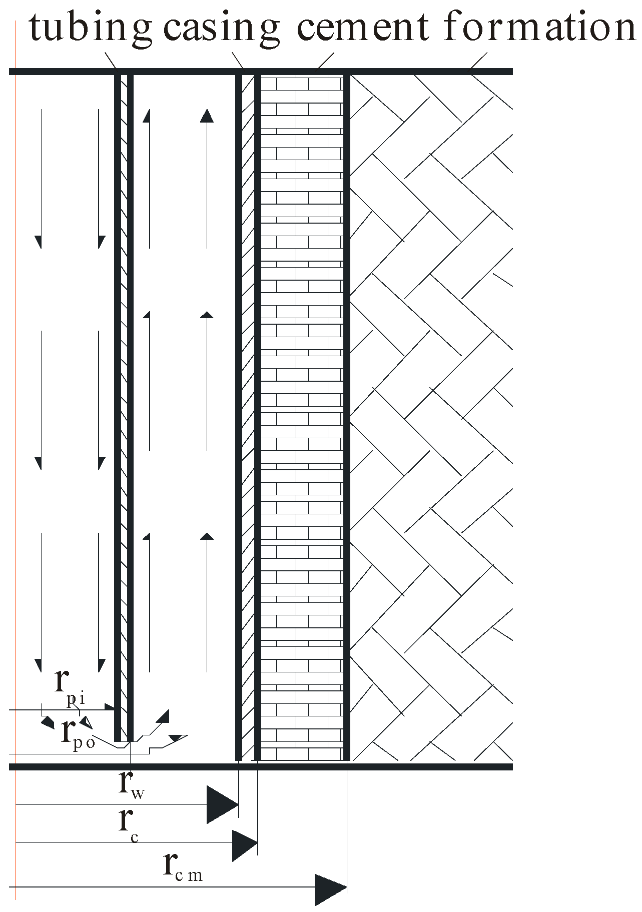
2.1.1. Assumed Condition of Model

To simplify the model, some assumed conditions of the model should be given based on the characteristic of actual wellbore heat transfer, which are (1) the axial heat conduction can be neglected compared with the axial heat convection; (2) there is no radial temperature gradient; (3) the formation temperature gradient and circulation rate remain constant; (4) the thermal properties of rock stay the same and do not change with the temperature and pressure; (5) the specific heat and heat conduction of rock perform isotropy; and (6) the temperature generated by pressure drop is neglected.

2.1.2. Mathematical Equations

The formation temperature is related not only to the well diameter, but also to the drilling time. Heat loss will decrease with time as the heat flow in the annulus tends to be stable. The heat transfer flux density between the annulus and formation can be considered as invariant. The equation of heat transfer from wellbore to the surroundings can be simplified to a 1-Dimension diffusivity issue if it only considers a very short section. The formation temperature surrounding the wellbore varies with radius and time can be calculated by the energy balance equation (Equation (1)) [21].

$$\frac{{\partial }^2{T}_f}{\partial r^2}+\frac{1}{r}\frac{\partial T_f}{\partial r}=\frac{{\rho }_f{c}_f}{k_f}\frac{\partial T_f}{\partial t}$$

(1)

where T_f is the formation temperature near the wellbore, °C; ${\rho }_f$ is the formation density, kg/m³; $c_f$ is the specific heat capacity of formation, J/(kg·°C); $k_f$ is the thermal conductivity of formation, W/(m·K); r is the radius, m.

To transform Equation (1) into dimensionless form, dimensionless radius, $r_D=r/r_w$, dimensionless time, $\alpha =k_f/{\rho }_f{c}_f$, $t_D=\alpha t/r_w^2$, dimensionless temperature T_D, the Kabir and Hasan Model [22] is used,

$$\begin{gathered} \frac{{\partial }^2{T}_e}{\partial r_D^2}+\frac{1}{r_D}\frac{\partial T_e}{\partial r_D}=\frac{\partial T_e}{\partial t_D} \\ \underset{r_D\to \infty }{\mathit{lim}}\frac{\partial T_e}{\partial r_D}=0 \\ {\frac{\partial T_e}{\partial r_D}|}_{r_D=1}=\frac{Q}{2\pi k_f} \end{gathered}$$

(2)

Equation (2) can be solved by Laplace transform. When r_D = 1, the temperature at the interface of the wellbore and formation is

$$\begin{gathered} T_w=T_{ei}+\frac{Q}{{\pi }^2{k}_f}I \\ I={{\displaystyle \int }}_0^{\infty }\frac{1-e^{-u^{2}tD}}{u^2}\frac{Y_1\left(u\right)J_0\left(u\right)-J_1\left(u\right)Y_0\left(u\right)}{J_1^2\left(u\right)+Y_1^2\left(u\right)} \end{gathered}$$

(3)

We define dimensionless temperature T_D, as

$$T_D=\frac{2\pi k_f}{Q}\left(T_w-T_{ei}\right)=-\frac{2I}{\pi }$$

(4)

The function of T_D was used to arrive at the following expression,

$$T_D=\{\begin{array}{c}1.1281\sqrt{t_D}(1-0.3\sqrt{t_D})\left(t_D\le 1.5\right)\\ \left(0.4063+0.5\mathrm{lnt}{t}_D\right)\left(1+0.6t_D\right)\left(t_D>1.5\right)\end{array}$$

(5)

To construct the easy-to-calculate wellbore temperature field model, a few assumptions should be listed: (1) the Joule-Thompson Effect of fluid in the wellbore is neglected; (2) it is homogeneous for rock in each formation layer, and the borehole diameter does not change with the depth; (3) the influence of frictional heat is neglected; (4) the phase of the fluid in the wellbore does not transform.

The annulus and pipe temperature differential model can be deduced according to the first law of thermodynamics and the basic principle of heat transfer [23].

$$\begin{gathered} \frac{d{T}_a}{dL}=\frac{1}{B}\left(T_a-T_p\right)-\frac{1}{A}\left(T_{\epsilon i}-T_a\right) \\ \frac{d{T}_p}{dL}=\frac{1}{B}\left(T_a-T_p\right) \\ A=\frac{C_m{Q\rho }_m\left(k_f{+r}_w{U}_a{T}_D\right)}{{2\pi r}_w{U}_a{k}_f} \\ B=\frac{C_m{Q\rho }_m}{{2\pi r}_{pi}{U}_p} \\ {U}_a=\frac{1}{r_w\left[\frac{1}{r_w{h}_a}+\frac{\ln \left(r_c/r_w\right)}{k_c}+\frac{\ln \left(r_{cm}/r_c\right)}{k_{cm}}\right]} \\ {U}_p=\frac{1}{r_{pi}\left[\frac{1}{r_{pi}{h}_{pi}}+\frac{\ln \left(r_{\mathit{po}}/r_{\mathit{pi}}\right)}{k_t}+\frac{1}{r_{\mathit{po}}{h}_{\mathit{po}}}\right]} \end{gathered}$$

(6)

where T_a is the drilling fluid temperature in the annulus, °C; T_p is the drilling fluid temperature in the pipe, °C; L is the well depth, m; Q is the drilling fluid flow rate, m³/s; $T_{\epsilon i}$ is the initial formation temperature, °C; U_a is the total convection coefficient between the annulus and formation, W/(m·K); C_m is the specific heat of the drilling fluid, W/(m·K); U_p is the total convection coefficient between the annulus and the pipe, W/(m·K); ${\rho }_m$ is the drilling fluid density at the depth of L in the well, kg/m³. $r_w$ is the inner radius of the wellbore, m; $r_c$ is the outer radius of the casing, m; $r_{cm}$ is the radius of cement, m; $r_{pi}$ is the inner radius of the pipe, m; $r_{po}$ is the outer radius of the pipe, m. $k_t$ is the thermal conductivity of the pipe, W/(m·K); $k_c$ is the thermal conductivity of the casing, W/(m·K); $k_{cm}$ is the thermal conductivity of cement, W/(m·K); $h_a$ is the convection heat transfer coefficient of the annulus, W/(m²·K); $h_{pi}$ is the convection heat transfer coefficient of the inner pipe, W/(m²·K); $h_{po}$ is the convection heat transfer coefficient of the outer pipe, W/(m²·K).

2.1.3. Initial and Boundary Conditions

The drilling fluid temperature of pipes and the annulus at the wellhead is known,

$$\begin{gathered} T_p\left(0,t\right)=T_{\mathit{in}} \\ {T}_a\left(0,t\right){=T}_{\mathit{out}} \end{gathered}$$

(7)

where T_in is the inlet temperature of the drilling fluid, °C; T_out is the outlet temperature of the drilling fluid, °C.

The drilling fluid temperature of the pipe and annulus at the well bottom is equal,

$$T_a\left(Z,t\right){=T}_p\left(Z,t\right)$$

(8)

where Z is the depth of the bottom hole, m.

Combining Equations (5)–(7) and Equation (8), the temperatures in the pipe and annulus can be calculated,

$$\begin{gathered} T_a{=\beta }_1{e}^{{\lambda }_{1}L}{+\beta }_2{e}^{{\lambda }_{2}L}+\frac{\mathit{GL}}{100}+T_s \\ {T}_p{=\beta }_1\left(1+B/A-{B\lambda }_1\right)e^{{\lambda }_{1}L}{+\beta }_2\left(1+B/A-{B\lambda }_2\right)e^{{\lambda }_{2}L}+\frac{G\left(L-B\right)}{100}{+T}_s \\ {\lambda }_1=\frac{1+\sqrt{1+4A/B}}{2A} \\ {\lambda }_2=\frac{1-\sqrt{1+4A/B}}{2A} \\ {T}_{\epsilon 1}{=T}_s+\frac{\mathrm{GL}}{100} \end{gathered}$$

(9)

where β₁, β₂ are modeling coefficients; G is the geothermal gradient, °C/100 m; $T_s$ is the surface temperature, °C.

2.2. Pressure Model in the Wellbore during Circulation

Five types of pressure, which are static pressure, annulus pressure drop, Initiating Circulation Pressure, viscous pressure, and inertial pressure, exist in the wellbore during the drilling. As listed in

Table 1. The pressure combination in different condition [24].

Conditions Partial Pressure		Hydrostatic Pressure	Frictional Pressure Loss	Initiating Circulation Pressure	Viscous Pressure	Inertial Wave
		ps	pf	pg	pV	pi
0	Standard static	+
1	pumping	+		+
2	circulation	+	+
3a	Trip out (acceleration)	+			-	-
3b	Trip out (constant)	+			-
3c	Trip out (decelerate)	+			-	+
4a	Trip in (acceleration)	+			+	+
4b	Trip in (constant)	+			+
4c	Trip in (decelerate)	+			+	-

“+” indicates that the pressure is downward; “-” indicates that the pressure is upward.

, the five types of pressure are not in the wellbore all the time; different pressure combinations appear in different drilling conditions.

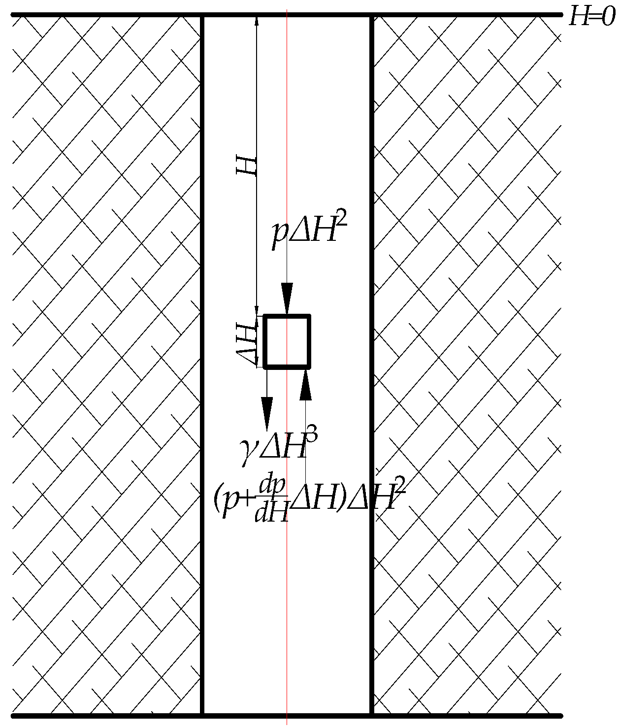
2.2.1. Pressure Gradient of Circulating Drilling Fluid in the Annulus

The pressure gradient of circulating drilling fluid in the annulus is given as follows [24],

$$\frac{{\mathit{dp}}_c}{\mathit{dL}}=\frac{{\mathit{dp}}_s}{\mathit{dL}}+\frac{{\mathit{dp}}_f}{\mathit{dL}}+\frac{{\mathit{dp}}_a}{\mathit{dL}}$$

(10)

where, the three terms of the right equation are hydrostatic pressure gradient, frictional pressure drop gradient and acceleration pressure gradient, respectively, L is length, m. The acceleration pressure gradient is somewhat smaller compared with the other two pressure gradients when the circulation is stable, so the pressure gradient is neglected and Equation (10) can be shortened as follows,

$$\frac{{\mathit{dp}}_c}{\mathit{dL}}=\frac{{\mathit{dp}}_s}{\mathit{dL}}+\frac{{\mathit{dp}}_f}{\mathit{dL}}$$

(11)

2.2.2. Hydrostatic Pressure Gradient

$$\frac{{\mathit{dp}}_s}{\mathit{dL}}{=\rho }_{m}g$$

(12)

where ρ_m is the drilling fluid density at depth z, kg/m³.

The static pressure can be expressed as ESD (equivalent static density),

$$ESD=\frac{p_{sz}-p_0}{gZ}$$

(13)

where $p_{sz}$ is the static pressure at the bottom, MPa; $p_0$ is the pressure at the surface, MPa.

Oil-based drilling fluid is generally considered that is not suitable for a geothermal well because oil-based drilling fluid may pollute the reservoir and reduce the production of the geothermal well. So, in this paper, water-based drilling fluid is used. A mathematical equation of the procedure of evaluating the density as a function of pressure and temperature is by [25],

$${\rho }_m{=\rho }_{m0}{\times e}^{\Gamma (p,T)}$$

(14)

where,

$${\Gamma (p,T)=\gamma }_p(p-p_0{)+\gamma }_{\mathit{pp}}{(p-p_0)}^2{+\gamma }_T(T-T_0{)+\gamma }_{\mathit{TT}}{(T-T_0)}^2{+\gamma }_{\mathit{pT}}(p-p_0)(T-T_0)$$

(15)

where ρ_m is the drilling fluid density under the condition of p and T, kg/m³; ρ_m0 is the drilling fluid density measured at the surface, kg/m³; p is the experiment pressure, Pa; p₀ is the atmosphere pressure, MPa; T is the experiment temperature, °C; T₀ is the temperature at the surface, the value is 15 °C; γ_p, γ_pp, γ_T, γ_TT and γ_pT are coefficients which should be determined, for different drilling fluids, from density measurement at elevated pressures and temperatures. As the effect of pressure on density is insignificant relative to the effect of temperature in the geothermal well, the effect factor to density simply considers temperature, and if we expand Equation (11) in a Taylors series, and neglect the pressure terms and all higher order terms, Equation (11) can be conversed as follows,

$${\rho }_m{=\rho }_{m0}[{1+\gamma }_T\left(T-T_0\right){+\gamma }_{\mathit{TT}}{\left(T-T_0\right)}^2]$$

(16)

2.2.3. Friction Pressure Loss

The rheological models generally used by drilling engineers to approximate fluid behavior are (1) the Newtonian model, (2) the Bingham plastic model, and (3) the power-law model. To determine the flow state of the drilling fluid, the Reynolds number N_Re should be calculated as follows,

$$N_{Re}=\frac{{\rho }_m\overline{v}d}{\mu }$$

(17)

For engineering application, flow of a Newtonian fluid in pipes is usually considered to be laminar if the Reynolds number is less than 2100 and turbulent if the Reynolds numbers is greater than 2100. As shown in

Table 2. The frictional pressure loss of a different rheological model under laminar in the pipe and annulus [26].

Position	Newtonian Model	Bingham Model	Power Law Model
Pipes	$\frac{d{p}_f}{dL}=31.92\frac{\mu \overline{v}}{d^2}$	$\frac{d{p}_f}{dL}=31.92\frac{{\mu }_p\overline{v}}{d^2}+52.3\frac{{\tau }_y}{d}$	$\frac{d{p}_f}{dL}=0.1571\frac{{(0.0254)}^{1+n}K{\overline{v}}^n{(\frac{3+1/n}{0.0416})}^n}{{(0.3048)}^n{d}^{1+n}}$
Annulus	$\frac{d{p}_f}{dL}=47.88\frac{\mu \overline{v}}{{(d_2-d_1)}^2}$	$\frac{d{p}_f}{dL}=47.88\frac{{\mu }_p\overline{v}}{{(d_2-d_1)}^2}+58.84\frac{{\mathsf{\tau }}_y}{d_2-d_1}$	$\frac{d{p}_f}{dL}=0.1571\frac{{(0.0254)}^{n+1}K{\overline{v}}^n{(\frac{2+1/n}{0.0208})}^n}{{(0.3048)}^n{(d_2-d_1)}^{1+n}}$

, a different rheological laminar model has a different frictional pressure drop gradient.

The frictional pressure loss expressions for all the three rheological models under turbulent conditions are the same. In the pipes, the frictional pressure loss is shown as follows,

$$\frac{d{p}_f}{dL}=2.44\frac{f{\overline{v}}^2{\rho }_m}{d}$$

(18)

The frictional pressure loss in the annular is,

$$\frac{d{p}_f}{dL}=2.99\frac{f{\overline{v}}^2{\rho }_m}{d_2-d_1}$$

(19)

where, f is the fanning friction factor; μ is the viscosity of the drilling fluid, mPa·s; is the average flow rate, m/s; τ_y is the sheer stress at the yield point, Pa; K is the velocity coefficient; d is the inner diameter of the pipe, m; d₁ is the outer diameter of the pipe, m; d₂ is the inner diameter of the casing, m.

2.2.4. Iterative Method to Solve the Pressure and Temperature Models

Suppose the wellbore consists of n overlying cylinder units and each unit’s length is Δz = Z/n. The temperature of the drilling fluid in each unit can be described as follows,

$$T_i=T\left(z_i\right)\left(i=1,2,3,\dots ,n\right)$$

(20)

Suppose the temperature, pressure and density of the drilling fluid are identical in each element of statics pressure, so the iteration equation of statics pressure is,

$$p_{i+1}{=p}_i+\Delta p_i{=p}_i+g\Delta z_i{\rho }_{\mathit{mi}}\left(i=1,2,3,\dots ,n\right)$$

(21)

The boundary conditions are,

$$p_s\left(z=0\right){=p}_0{,T}_s\left(z=0\right){=T}_0$$

(22)

So the static pressure in the annulus is,

$$p_s-p_0=g{\displaystyle \sum }_{i=1}^n{\rho }_{\mathit{mi}}\Delta z_i$$

(23)

The calculation model of ESD is expressed as follows,

$$\mathit{ESD}=\frac{p_s-p_0}{\mathit{gz}}=\frac{1}{z}{\displaystyle \sum }_{i=1}^n{\rho }_{\mathit{mi}}\Delta z_i$$

(24)

Combining Equations (20) and (21), the ECD is shown as follows,

$$\mathit{ECD}=\mathit{ESD}+\frac{p_f}{\mathit{gz}}=\frac{1}{z}{\displaystyle \sum }_{i=1}^n{\rho }_{\mathit{mi}}\Delta z_i+\frac{p_f}{\mathit{gz}}$$

(25)

2.3. Surge Pressure

Casing running is the first step during cementing, and casing running surge pressure may induce weak formation leakage and cause a downhole problem. According to this problem, the calculation model of casing running surge pressure was established.

2.3.1. Initiating Circulation Pressure

Drilling fluid usually exhibits a thixotropic behavior when the circulation starts. The pressure gradient required to start the circulation can be computed if the gel strength of the drilling fluid is known. Since the shear stress is greatest at the pipe wall, this is where the initial fluid movement will occur. Equating the wall shear stress to the gel strength yields,

$${\tau }_g=\frac{r_{\mathit{pi}}}{2}\frac{{\mathit{dp}}_g}{\mathit{dL}}\left(pipe\right)$$

(26)

and

$${\tau }_g=\frac{\left(r_w-r_{po}\right)}{2}\frac{{\mathit{dp}}_g}{\mathit{dL}}\left(annulus\right)$$

(27)

where τ_g is the gel strength, Pa.

Changing from consistent units to field units and solving for pressure dp_f/dL gives

$$\frac{{\mathit{dp}}_g}{\mathit{dL}}=\frac{{\tau }_g}{2500d}$$

(28)

and

$$\frac{{\mathit{dp}}_g}{\mathit{dL}}=\frac{{\tau }_g}{2500\left(d_2-d_1\right)}$$

(29)

2.3.2. Inertial Effects

The pressure change in a fluid due to inertial effects can be estimated from consideration of the vertical forces acting on a cube of the fluid at a depth H. As shown in Figure 2, the force is not to be at rest but accelerating in a downward direction. The sum of the downward forces must be equal to the mass of the fluid element multiplied by its acceleration [27].

$$p\Delta H^2-(p+\frac{\mathit{dp}}{\mathit{dD}}\Delta H)\Delta H^2+\gamma \Delta H^3=\rho \Delta H^{3}a$$

(30)

where $\gamma$ is the unit weight, N/m³.

Simplifying the expression above, we can get the expression below,

$$\frac{\mathit{dp}}{\mathit{dD}}{=F}_{w\nu }-\mathit{pa}$$

(31)

If the magnitude of the pressure gradient due to fluid acceleration is the only pressure of interest, then,

$$\frac{\mathit{dp}}{\mathit{dL}}=\mathit{pa}$$

(32)

For a pipe with a closed end in an incompressible fluid, the relation between fluid acceleration and pipe acceleration is given by,

$${a=a}_p\frac{d_1^2}{d_2^2-d_1^2}$$

(33)

$$\frac{{\mathit{dp}}_i}{\mathit{dL}}=\frac{0.00366\rho a_p{d}_1^2}{d_2^2-d_1^2}$$

(34)

where a_p is the tripping acceleration, m/s².

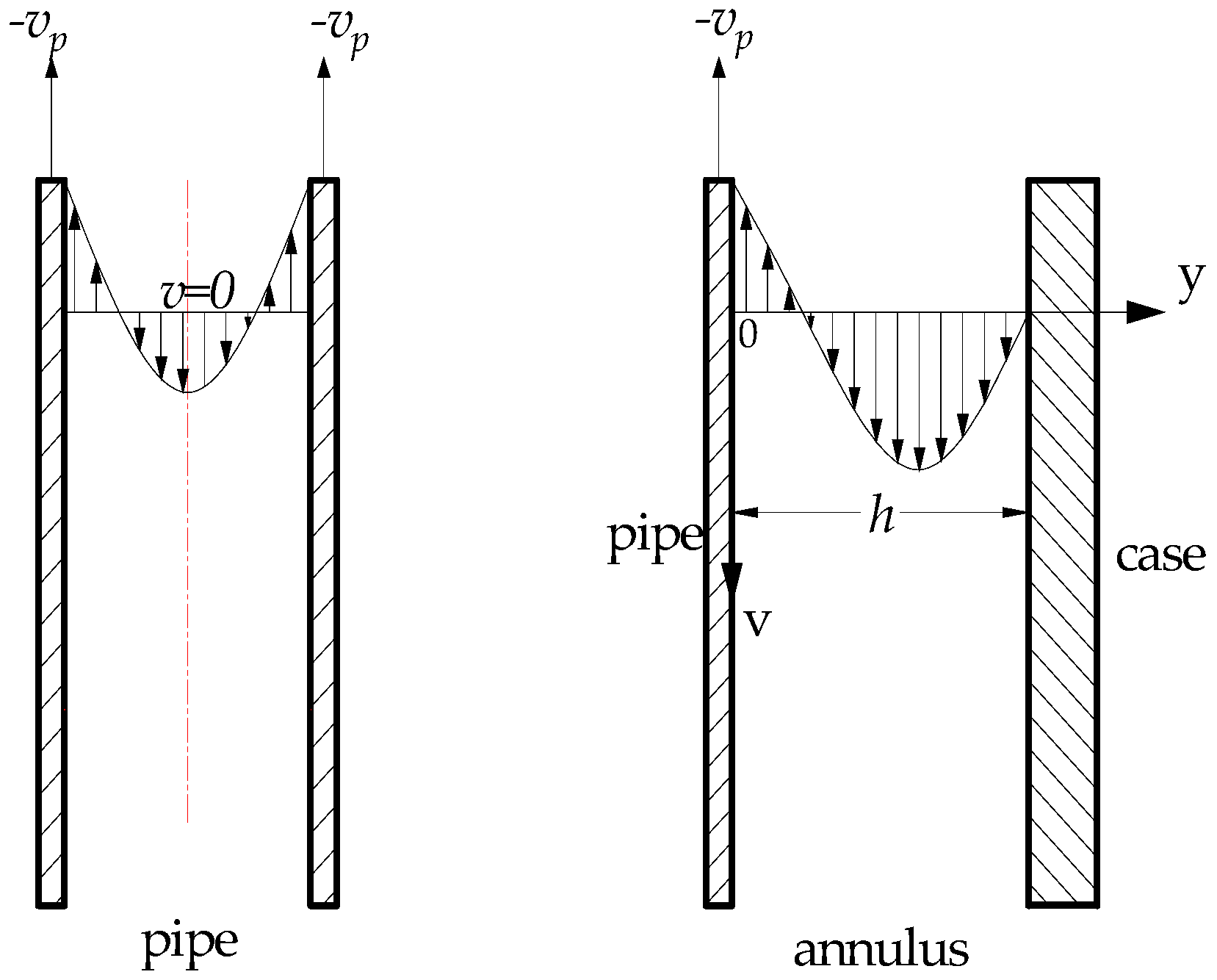
2.3.3. Viscous Pressure Due to Vertical Pipe Movement

As the pipe is moved downward in a well, the drilling fluid must move upward to exit the region being entered by the new volume of the extending pipe. Likewise, an upward pipe movement requires a downward fluid movement. The flow pattern of the moving fluid can be either laminar or turbulent depending on the velocity at which the pipe is moved. It is possible to derive mathematical equations for surge and swab pressure only for the laminar flow pattern. Empirical correlations must be used if the flow pattern is turbulent.

A typical velocity profile for laminar flow caused by pulling the pipe out of the hole at velocity, −υ_p, is shown in Figure 3. Note that the velocity profile inside the inner pipe caused by a vertical pipe movement is identical to the velocity profile caused by pumping fluid down the inner pipe. If the mean fluid velocity in the pipe is expressed relative to the pipe wall, the viscous pressure in pipes can be expressed as follows,

$$\frac{d{p}_v}{dL}=\frac{\mu ({\overline{v}}_i+{\mathrm{v}}_p)}{1500d^2}$$

(35)

where ${\overline{v}}_i$ is average rate relative to pipes, m/s.

The velocity profile in the annulus caused by vertical pipe movement differs from the velocity profile caused by pumping fluid through the annulus in that the velocity at the wall of the inner pipe is not zero [28]. The velocity for slot flow is given by,

$$\nu =\frac{1}{2\mu }\frac{{\mathit{dp}}_v}{\mathit{dL}}(\mathit{yh}-y^2)-{\nu }_p(1-\frac{y}{h})$$

(36)

where h is the wide between pipe wall and case wall, m.

The constants of integrations, τ₀ and υ₀, can be evaluated as the boundary conditions

$$\{\begin{array}{c}\nu =-{\nu }_p,\mathit{at}y=0\\ \nu =0,\mathit{at}y=h\end{array}$$

(37)

Applying these boundary conditions yields

$$\{\begin{array}{c}-{\nu }_p=0-{0+\nu }_0\\ 0=\frac{-h^2}{2\mu }\frac{{\mathit{dp}}_v}{\mathit{dL}}-{\tau }_0\frac{h}{\mu }{+\nu }_0\end{array}$$

(38)

The flow rate q can be described as follow,

$$q=\nu \mathit{dA}=\nu \pi (r_w+r_{pi})dy$$

(39)

The expression for laminar flow due to the vertical movement of an open-ended pipe of uniform cross-sectional area in a Newtonian fluid is shown as follows,

$$\begin{array}{l}{\overline{v}}_a=v_p\frac{3d^4-4d_{pi}^2{(d_{ci}-d_{pi})}^2}{6d^4-4{(d_{ci}-d_{pi})}^2(d_{ci}^2-d_{pi}^2)}(\mathrm{open}-\mathrm{ended})\\ {\overline{v}}_a={\nu }_p\frac{d_{ci}^2}{(d_{ci}^2-d_{pi}^2)}(\mathrm{open}-\mathrm{ended})\end{array}$$

(40)

where $d_{\mathit{ci}}$ is diameter of pipe, m; $d_{\mathit{pi}}$ is the diameter of inner case, m.

The viscous pressure gradient is given,

$$\frac{d{p}_v}{dL}=\frac{\mu ({\overline{v}}_a+\frac{v_p}{2})}{1000{(d_{ci}-d_{pi})}^2}$$

(41)

For the non-Newtonian rheological model, the resulting surge pressure equations are far too complex for field application. A simplified technique for computing surge was presented by Burkhardt [29]. The simplified method is based on the use of an effective fluid velocity in the annular flow equation. An effective mean annular velocity is given by,

$${\overline{v}}_{a\epsilon }=\overline{v}+K{v}_p$$

(42)

where K is the mud clinging constant, of which given by Fontenot [30].

$$\begin{gathered} K=\frac{\sqrt{\frac{a^4+a}{1+a}}-a^2}{1-a^2}, \left(\mathrm{turbulent}\right) \\ K=\frac{a^2-2a^{2}lna-1}{2\left(1-a^2\right)lna}, \left(\mathrm{laminar}\right) \end{gathered}$$

(43)

where a is ratio of pipe diameter to hole diameter.

3. Result and Discussion

The first production well ZK212, which has been drilled to exploit the deep reservoir in 2012 and 2013, is selected as the example. This well was drilled to a depth of 1508 m without any kick or blowout, but some fluid leak-off or loss occurred that was affected by the circulating temperature; the input temperature of the drilling fluid is 25 °C. The temperature of the bottom hole is 235 °C calculated by a SiO₂ geothermometer. The mean temperature gradient is 14 °C/100 m. The thermodynamics properties of materials in the wellbore and formation are listed in Table 1 and the fresh water from the river was used as the drilling fluid. According to the previous study [31], the height of the ZK212 to the zero point was −11.87 m, which means that the pore pressure was lower than the hydrostatic pressure. The density of the water varies with temperature, shown as follows,

$${\rho }_m=1014\times \left[1-4.536{\times 10}^{-4}\left(T-15\right)-1.972{\times 10}^{-6}{\left(T-15\right)}^2\right]$$

(44)

The ZK212 has a 245 mm string to 600 m. It is completed as an open hole from the 245 mm casing shoe to the bottom. The pump capacity for the drilling fluid is 40 m³/h. The Thermodynamics parameters and sizes of each section in the well are shown in

Table 3. Thermodynamics properties of the materials and formation.

Name	Density (kg/m3)	Thermal Conductivity (W/(m·K))	Thermal Capacity (J/(kg·°C)
Sandstone	2231	1.869	711.76
Basalt	1579	2.008	879.23
Granite	2641	2.821	837.36
Cement	2100	1.454	879.23
Casing	7848	45.174	460.55

and

Table 4. The inner and outer diameter of the casing, pipe, and cement.

Materials	Inner Diameter (mm)	Outer Diameter(mm)
pipe	139	159
casing	245	311
cement	311	406

respectively.

The wellbore temperature distribution in the ZK212 can be calculated based on the mathematical model and numerical solution.

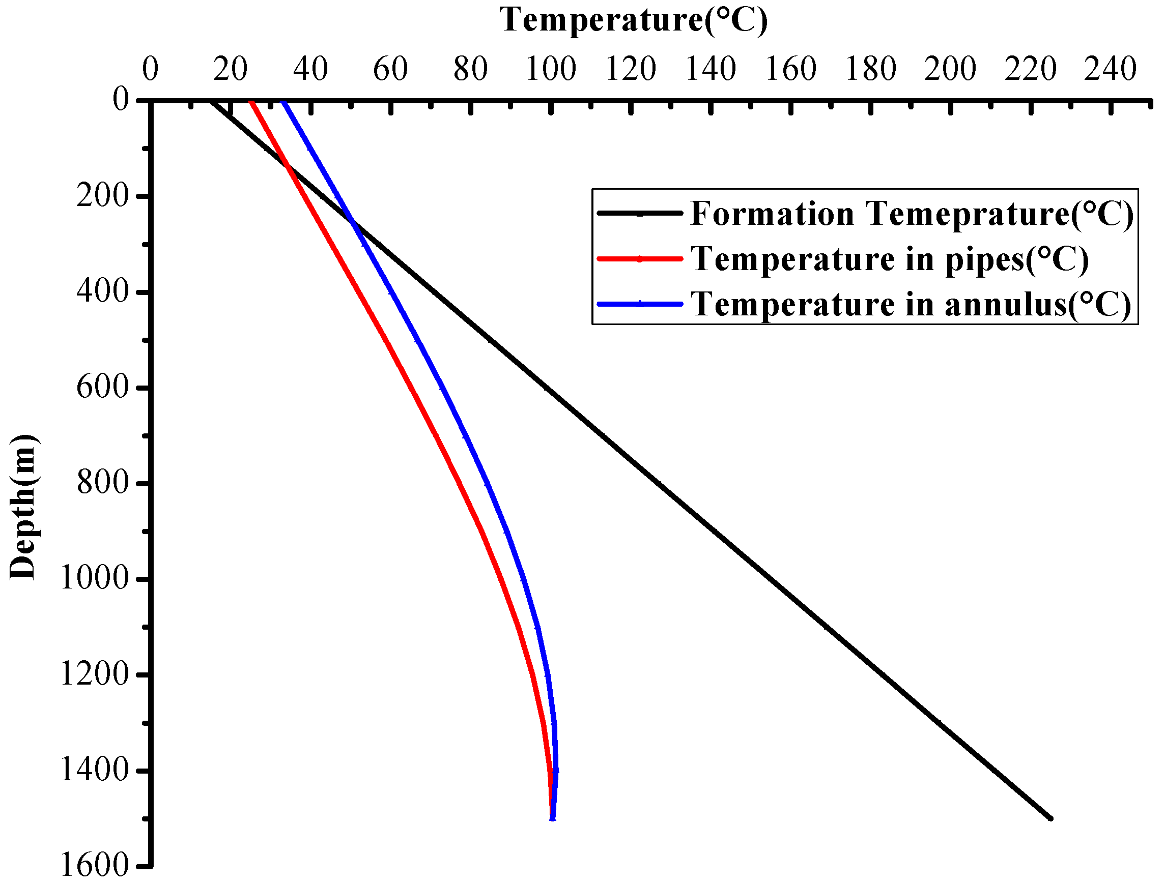
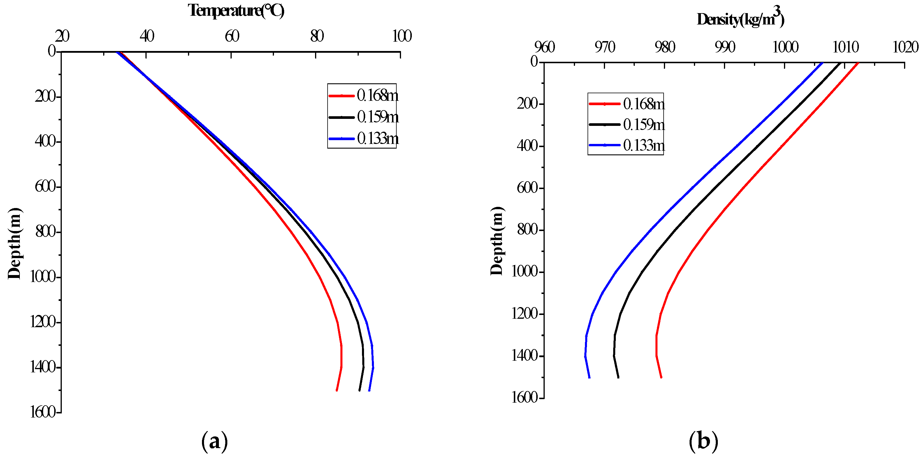
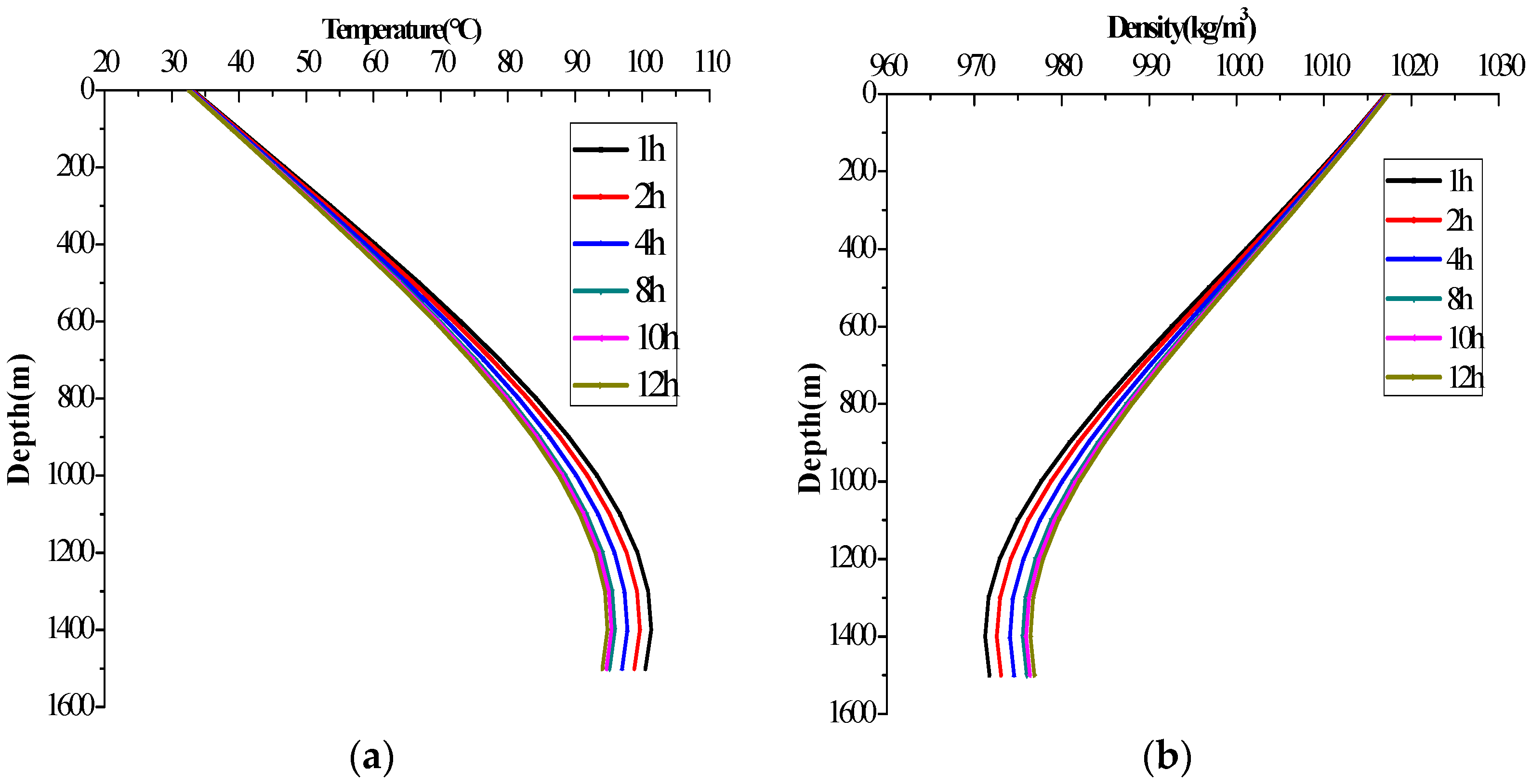
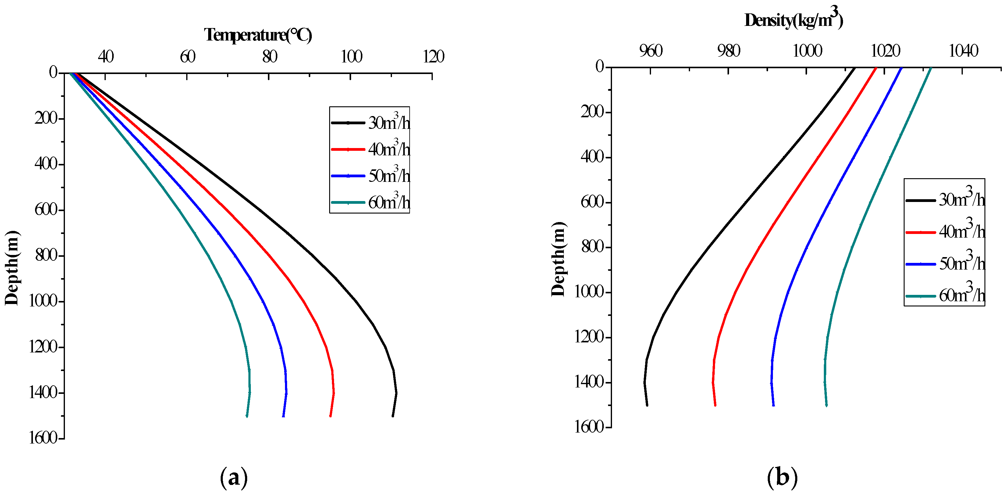
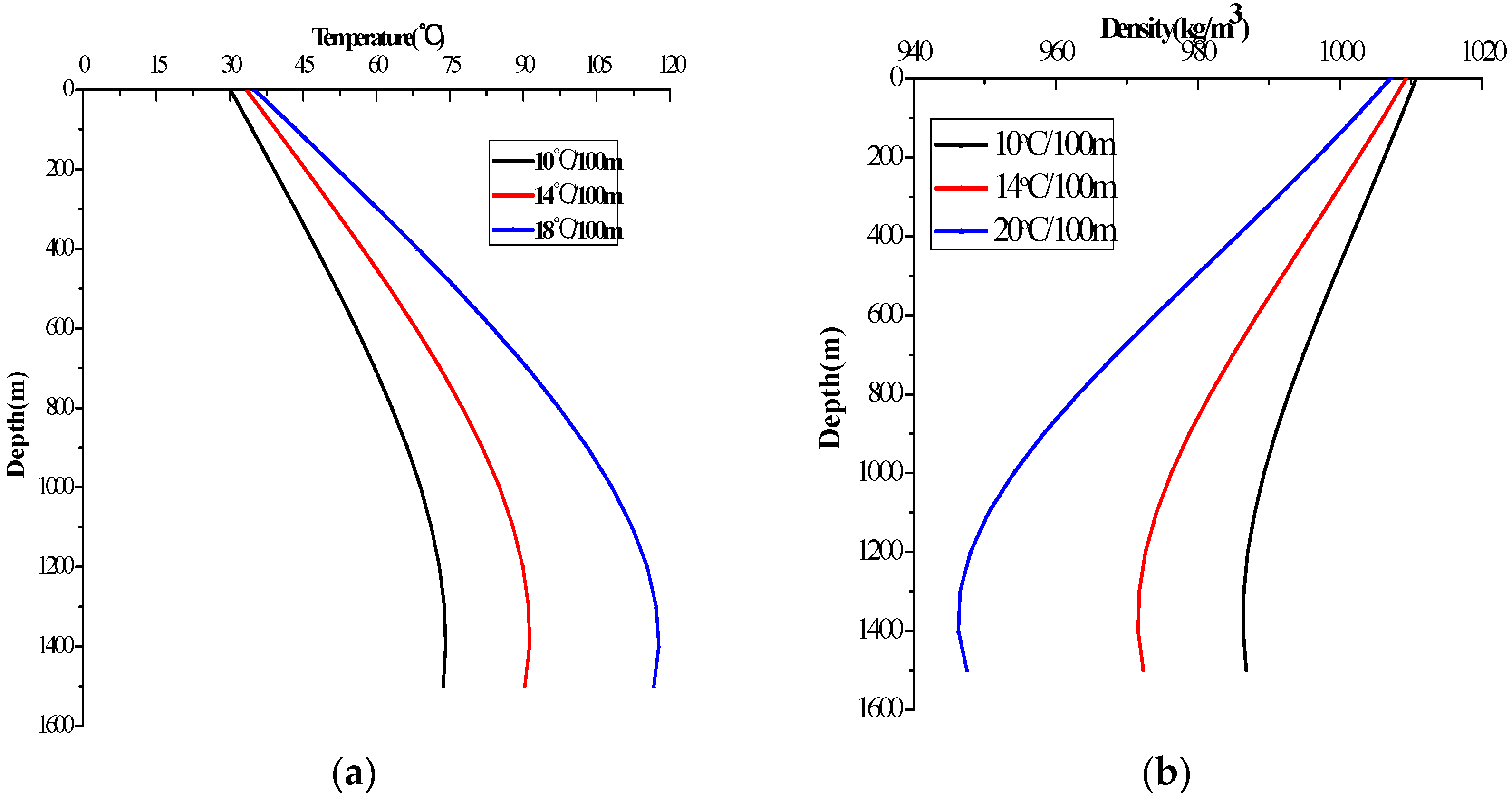
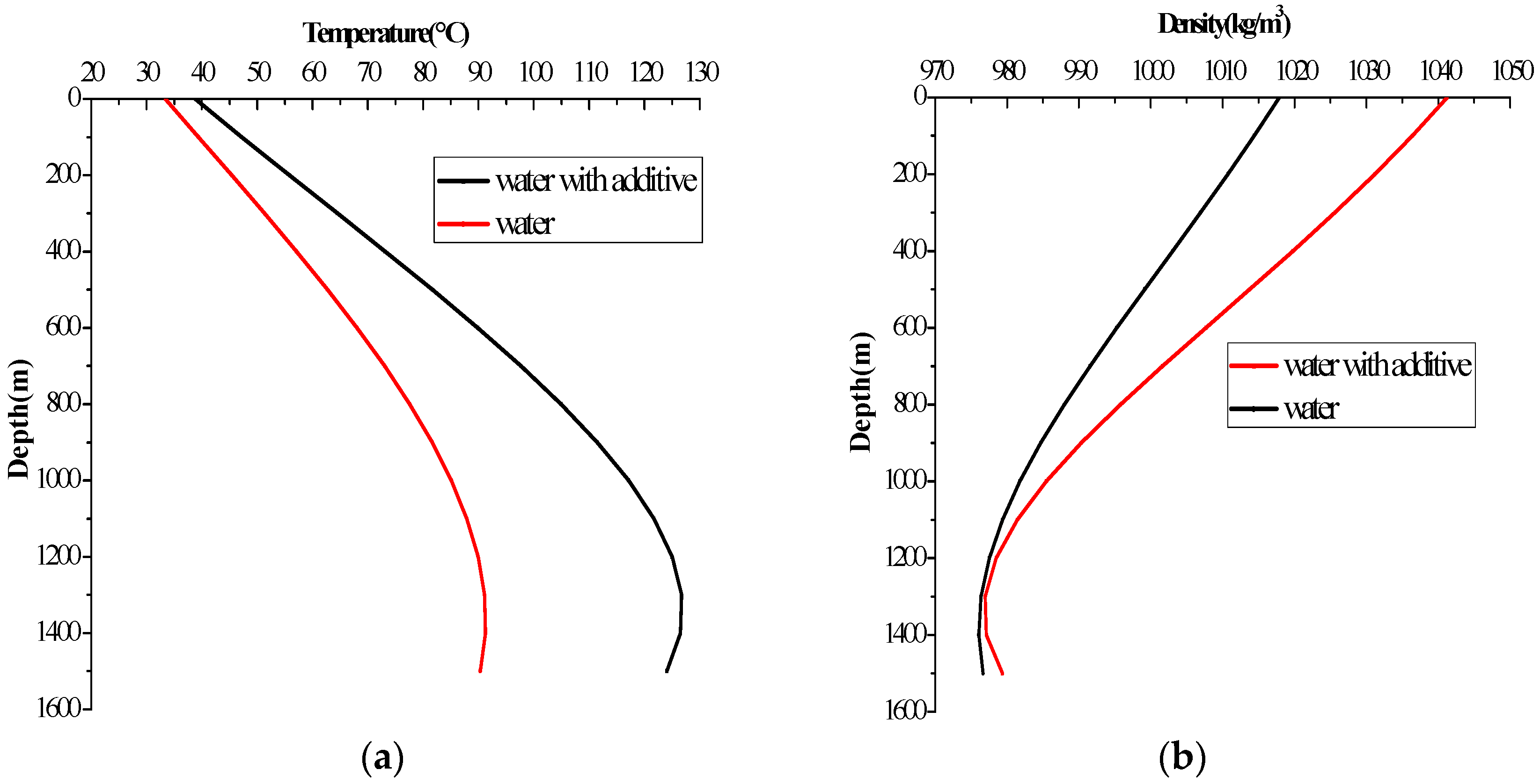
3.1. Temperature and ECD Distribution in the Wellbore

As shown in Figure 4, the formation was heated from the surface to 300 m, then cooled to the bottom. The location of the highest fluid temperature is at a point above the well bottom in the annulus; it is not at the well bottom because of the high formation temperature influence when the fluid rises from the bottom.

Figure 5a is the relation curve of the drilling fluid temperature in the annulus and circulation time. It is illustrated that the circulation time has a strong influence on the annular temperature, when other parameters remain constant. As the circulation time grows, the impact on annular temperature wears off and the highest temperature in the annulus moves upward. The change of temperature becomes slow after 8 h circulation. Figure 5b shows that the variations of the ECD with circulation are parallel to the annular temperature. The circulation time only influences the density of the drilling fluid through the temperature. The ECD tends to remain stable with the circulation time.

The relations of the drilling fluid temperature in the annulus and the flow rate are shown in Figure 6a. The flow rate is connected with the strength of convection, which has a large influence on the distribution of temperature in the wellbore because of the high temperature. The larger velocity of the drilling fluid flows into the well, while the lower temperature distributes into the annulus. Figure 6b expresses the ECD in the annulus with depth under a different flow rate. Big differences exist in the different flow rate; there is a positive correlation between the flow rate and the ECD, as the flow rate effect not only changes the density, but also the friction pressure loss.

The geothermal gradient is another important parameter to temperature distribution in the annulus (Figure 7a). The geothermal gradient increases 42.9% or decreases 28.6%, the temperature of the bottom hole elevates 20 °C or reduces 30 °C. The ECD distributions in the annulus under various geothermal gradients differ greatly (Figure 7b). It is obvious that an inaccurate geothermal gradient will lead to a large error in predicting the temperature distribution and calculating the ECD in the annulus.

Figure 8a demonstrates that the annular diameter affects the temperature distribution in the annulus. Assume that the wellbore diameter keeps constant; the diameters of the pipe are 133 mm, 159 mm and 168 mm respectively. The result indicates that the temperature in the annulus reduces as the annular diameter decreases; as the flow rate in the small annular diameter is faster than in the large annular diameter, the cooling performance enhances. The temperature in the shallow well part is little affected. The ECDs under a different annular diameter represent obvious variance in both the shallow and deep part of the well; f variation of the annular diameter causes the flow rate change, which induces the friction pressure loss in the annulus (Figure 8b).

Loss of circulation is a common problem during the drilling. To prevent the problem and keep the pressure balance in the wellbore, some additives should be added to the drilling fluid, which will change the fluid model and physical properties and temperature distribution of the wellbore. The additive is added in the drilling fluid when drilled to the leakage layer, which varies the properties of the drilling fluid relative to the initial one. Kaolinite was added in water to maintain the safe drilling, the density and viscosity, thermal conductivity and thermal capacity reach to 1030 kg/m³, 98 mPa·s, 1.731 W/(m·K) and 1256 J/(kg·°C) respectively. The drilling fluid turns into the Bingham model, and the calculated N_Re is 384. As shown in Figure 9a, the temperature of the Bingham model in the wellbore is much higher than the temperature of the primary Newtonian model, so it is important to note that the temperature in the wellbore will shift after adding additives. Figure 9b shows that the ECD of the drilling fluid to which additives are added has a wide range of variation which is from 976 kg/m³ to 1042 kg/m³. The position of highest ECD with additives is at the wellhead and it is higher relative to that of primary drilling fluid without additives.

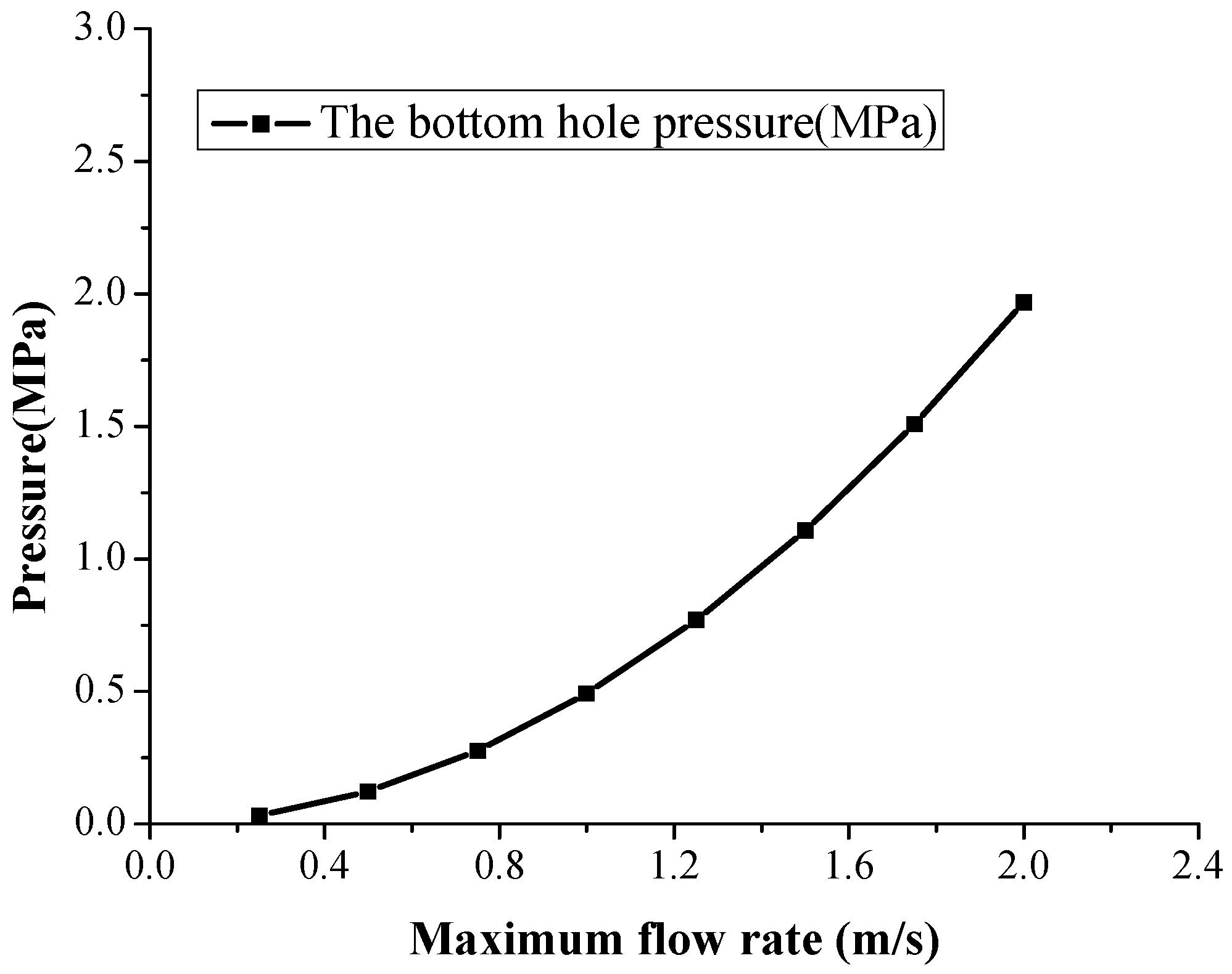
3.2. Surge Pressure Analysis

The movement of the pipes can be considered as a process of acceleration, constant speed and deceleration. The acceleration is 0.5 m/s², and the maximum rate of the pipes is 2 m/s. In this study, the stable method is adopted to analyze the surge method in the well.

Suppose other parameters remain constant except the velocity of pipes tripping in the well. Figure 10 illustrates that the surge pressure of bottom hole increases with the velocity of pipes tripping; the bottom hole pressure under the pipes tripping velocity of 0.25 m/s is 0.03 MPa and the pressure is up to 1.97 MPa when the velocity of pipes tripping reaches to 2 m/s.

Presume that the rate at which the pipes trip in the well is 2 m/s and other parameters remain the same. As the pipes trip in the hole from the depth of 300 m to the bottom hole and from the depth of 1200 m to the bottom hole, the surge pressure are seen in

Table 5. Surge pressure at the bottom hole as the pipes trip in under different depths.

Depth (m)	300	500	800	1000	1200
Surge pressure (MPa)	1.57	1.31	0.92	0.66	0.39

which increases from 0.39 MPa to 1.29 MPa.

Assume that the diameter of the wellbore can regulate, and the other diameters stay the same. As seen in

Table 6. Surge pressure at the bottom hole as the pipes trip in under different wellbore diameters.

Diameter (m)	0.216	0.245	0.265	0.290	0.311
Surge pressure (MPa)	1.97	0.69	0.42	0.26	0.19

, the larger the diameter of the wellbore is, the lower the surge pressure obtained. The diameter of the wellbore has significant influence on the surge pressure.

4. Conclusions

Pressure and temperature are crucial parameters for well drilling, and temperature should be considered when building the wellbore distribution under different conditions, as the density and rheology of the drilling fluid change with the temperature. This paper modeled the temperature distribution by the Hasan model, and a simulation of sensitivity analysis was also completed. The result indicates that the temperature of the drilling fluid in the bottom hole is much higher than the surface temperature; changing some parameters will lead to temperature redistribution in the wellbore. According to the sensitivity analysis, the geothermal gradient and flow rate are the most important parameters to temperature distribution. Circulation time and diameter of the wellbore also affect the temperature distribution, while the influence will gradually recede as the parameters increase; the wellbore temperature should be recalculated when primitive drilling fluid adds additives to maintain the wellbore stability as the properties have changed.

The ECD is affected by the temperature. Research shows that the rheological models, diameter of the wellbore, the geothermal gradient and flow rate all have a great influence on the ECD, especially the flow rate and geothermal gradient. The ECD has a large relation with the circulation time in the transient period, while gradually the ECD has no influence on circulation time as the drilling fluid become steady.

The surge pressure caused by casing running will be generated during cementing. According to the study, the velocity and depth of pipes tripping and the diameter of the wellbore are important parameters to the surge pressure.

References

1. Ali, K.V.; Eric, V.O. Early kick detection and well control decision-making for managed pressure drilling automation. J. Nat. Gas Sci. Eng. 2015, 27, 354–366. [Google Scholar]
2. Yu, J.Y.; Bai, Z.X.; Zheng, X.H.; Zhou, D.; Li, F.Y. Controlled Pressure Drilling and the Application in High-temperature Geothermal Exploration. Explor. Eng. 2013, 40, 19–23. [Google Scholar]
3. Wang, Z.Y.; Tang, S.R.; Zhou, S.G. Drilling and completion well techniques in Yangbajain Geothermal Field, Tibet. Explor. Eng. 1985, 5, 58–60. [Google Scholar]
4. Ansari, A.M.; Sylvester, N.D.; Sarica, C.; Shoham, O.; Brill, J.P. A Comprehensive Mechanistic Model for Upward Two-Phase Flow in Wellbores. SPE Prod. Facil. 1994, 9, 143–151. [Google Scholar] [CrossRef]
5. Peter, P.; Acuna, J.A. Implementing Mechanistic Pressure Drop Correlations in Geothermal Wellbore Simulators. In Proceedings of the World Geothermal Congress, Bali, Indonesia, 25–29 April 2010; pp. 25–29.
6. Li, S.G.; Deng, J.G.; Wei, B.H.; Yu, L.J. Formation Fracture Pressure Calculation in High Temperatures Wells. Chin. J. Rock Mech. Eng. 2005, 24, 5669–5673. [Google Scholar]
7. Zhong, B.; Shi, T.H.; Fang, D. Study of Pressure Balance in Deep Drilling Well. J. Southwest Pet. Inst. 1998, 20, 56–60. [Google Scholar]
8. Fan, H.H.; Liu, X.S. Study on the calculation model of steady fluctuation pressure in vertical well. Oil Drill. 1993, 15, 13–18. [Google Scholar]
9. Tao, Q.; Xia, H.N.; Peng, M.Q.; Li, B. Research on Surge Pressure of Casing Running in High-Temperature High-Pressure Oil Well. Fault Block Oil Gas Field 2006, 13, 58–61. [Google Scholar]
10. Fu, H.C.; Liu, Y.; Sun, Z.; Ma, Y.; Ai, Z. Calculation Model of Casing Running Surge Pressure and Influence Factors Analysis. Drill. Prod. Technol. 2013, 36, 15–18. [Google Scholar]
11. McMordie, W.C.; Bland, R.G.; Hauser, J.M. Effect of Temperature and Pressure on the Density of Drilling Fluids. In Proceedings of the SPE Annual Technical Conference and Exhibition, New Orleans, LA, USA, 26–29 September 1982; pp. 1–7.
12. Hoberock, L.L.; Thomas, D.C.; Nickens, H.V. Here’s How Compressibility and Temperature Affect Bottom-Hole Mud Pressure. Oil Gas J. 1982, 12, 159–164. [Google Scholar]
13. Harris, O.O.; Osisanya, S.O. Evaluation of Equivalent Circulation Density of Drilling Fluid under High-Pressure/High-Temperature Conditions. In Proceedings of the SPE Annual Technical Conference and Exhibition, Dallas, TX, USA, 9–12 October 2005; pp. 1–6.
14. Wang, H.G.; Liu, Y.S.; Yang, L.P. Effect of Temperature and Pressure on drilling Fluid Density in HTHP wells. Drill. Prod. Technol. 2000, 23, 56–60. [Google Scholar]
15. Ramey, H.J. Wellbore heat transmission. J. Pet. Technol. 1962, 14, 427–435. [Google Scholar] [CrossRef]
16. Sagar, R.K.; Dotty, D.R.; Schmidt, Z. Predicting temperature profiles in a flowing well. SPE Prod. Eng. 1991, 11, 441–448. [Google Scholar] [CrossRef]
17. Willhite, G.P. Over-all heat transfer coefficients in steam and hot water injection wells. J. Pet. Technol. 1967, 5, 607–615. [Google Scholar] [CrossRef]
18. Hasan, A.R.; Kabir, C.S. Modeling two-phase fluid and heat flows in geothermal wells. J. Pet. Sci. Eng. 2009, 71, 77–86. [Google Scholar] [CrossRef]
19. Raymond, L.R. Temperature distribution in a circulating drilling fluid. J. Pet. Technol. 1969, 3, 333–341. [Google Scholar] [CrossRef]
20. Yang, X.S.; Li, S.; Yan, J.N.; Lin, Y.X.; Wang, X. Temperature Pattern Modelling and Calculation and Analysis of ECD for Horizontal Wellbore. Drill. Fluid Complet. Fluid 2014, 31, 63–66. [Google Scholar]
21. Hagoort, J.; Assocs, B.V. Ramey’s Wellbore Heat Transmission Revisited. SPE J. 2004, 9, 465–474. [Google Scholar] [CrossRef]
22. Kabir, C.S.; Hasan, A.R.; Kouba, G.E.; Ameen, M. Determining Circulating Fluid Temperature in Drilling, Workover, and Well Control Operations. SPE Drill. Complet. 1996, 11, 74–79. [Google Scholar] [CrossRef]
23. Hasan, A.R.; Kabir, C.S. Aspects of Wellbore Heat Transfer during Two-Phase Flow. SPE Prod. Facil. 1994, 9, 211–216. [Google Scholar] [CrossRef]
24. Moore, P.L. Drilling Practices Manual; Petroleum Publishing Co.: Tulsa, OK, USA, 1974; pp. 114–123. [Google Scholar]
25. Cinar, M.; Onur, M.; Satman, A. Development of a Multi-feed P-T Wellbore Model for Geothermal Wells. In Proceedings of the Thirty-First Workshop on Geothermal Reservoir Engineering, Stanford University, Stanford, CA, USA, 30 January–1 February 2006; pp. 1–6.
26. Yu, H. Study the Wellbore fluctuation Pressure during Tripping Operation. Master’s Thesis, Southwest Petroleum University, Chengdu, China, 2014. [Google Scholar]
27. Karstad, E.; Aadnoy, B.S. Density Behavior of Drilling Fluids During High Pressure High Temperature Drilling Operations. In Proceedings of the IADC/SPE Asia Pacific Drilling Technology, Jakarta, Indonesia, 7–9 September 1998; pp. 227–237.
28. Bourgoyne, A.T.; Chenevert, M.E.; Young, F.S. Applied Drilling Engineering; Society of Petroleum Engineers: Richardson, TX, USA, 1986; pp. 114–165. [Google Scholar]
29. Burkhardt, J.A. Wellbore Pressure Surges Produced by Pipe Movement. J. Pet. Technol. 1961, 13, 559–565. [Google Scholar] [CrossRef]
30. Fontenot, J.E.; Clark, R.K. An Improved Method for Calculating Swab and Surge Pressures and Circulating Pressures in a Drilling Well. Soc. Pet. Eng. J. 1972, 14, 451–462. [Google Scholar] [CrossRef]
31. Zheng, X.H.; Liu, H.Y.; Ji, R.S.; Bai, Z.X. Pressure Analysis of ZK212 Well of Yangyi High Temperature Geothermal Field (Tibet, China). In Proceedings of the 6th International Conference on Applied Energy, Taipei, Taiwan, 30 May–2 June 2014; pp. 1793–1798.
Figure 1. Circulation model parameter in the wellbore.
Energies 10 00268 g001
Figure 2. Forces acting on a fluid element.
Energies 10 00268 g002
Figure 3. Velocity profiles for the laminar flow pattern when the pipe is pulled out of the well.
Energies 10 00268 g003
Figure 4. The temperature profile in the pipe and annulus (circulating 1 h).
Energies 10 00268 g004
Figure 5. Temperature (a) and ECD (b) in the annulus with the circulation time.
Energies 10 00268 g005
Figure 6. Temperature (a) and ECD (b) in the annulus with the flow rate (circulating 8 h).
Energies 10 00268 g006
Figure 7. Temperature (a) and ECD (b) in the annulus with the geothermal gradient (circulating 8 h).
Energies 10 00268 g007
Figure 8. Temperature (a) and ECD (b) in the annulus with the outer diameter of the pipe (circulating 8 h).
Energies 10 00268 g008
Figure 9. Temperature (a) and ECD (b) in the annulus with the rheological model of the pipe (circulating 8 h).
Energies 10 00268 g009
Figure 10. The bottom bole pressure with different rates of trip in.
Energies 10 00268 g010