
Data-Driven Predictive Torque Coordination Control during Mode Transition Process of Hybrid Electric Vehicles


1
School of Information and Electronic Engineering, Shandong Technology and Business University, Yantai 264005, China
2
School of Control Science and Engineering, Shandong University, Jinan 250061, China
*
Author to whom correspondence should be addressed.
Energies 2017, 10(4), 441; https://doi.org/10.3390/en10040441
Submission received: 16 November 2016
/
Revised: 20 March 2017
/
Accepted: 22 March 2017
/
Published: 1 April 2017
(This article belongs to the Special Issue Advanced Energy Storage Technologies and Their Applications (AESA))
Abstract
:Torque coordination control significantly affects the mode transition quality during the mode transition dynamic process of hybrid electric vehicles (HEV). Most of the existing torque coordination control methods are based on the mechanism model, whose control effect heavily depends on the modeling accuracy of the HEV powertrain. However, the powertrain structure is so complex, that it is difficult to establish its precise mechanism model. In this paper, a torque coordination control strategy using the data-driven predictive control (DDPC) technique is proposed to overcome the shortcomings of mechanism model-based control methods for a clutch-enabled HEV. The proposed control strategy is only based on the measured input-output data in the HEV powertrain, and no mechanism model is needed. The conflicting control requirements of comfortability and economy are included in the cost function. The actual physical constraints of actuators are also explicitly taken into account in the solving process of the data-driven predictive controller. The co-simulation results in Cruise and Simulink validate the effectiveness of the proposed control strategy and demonstrate that the DDPC method can achieve less vehicle jerk, faster mode transition and smaller clutch frictional losses compared with the traditional model predictive control (MPC) method.
1. Introduction
The multi-energy powertrain system is the most distinctive feature that makes hybrid electric vehicle (HEV) more energy efficient than the traditional vehicle, and its key technology directly determines the economy, reliability, safety and comfortability in HEV. The control of the HEV multi-energy powertrain system can be classified into two kinds of core problems. The first is the energy distribution and efficiency optimization of multi-energy sources, and the second is the dynamic torque coordination between the multi-power sources. The former aims to improve the fuel economy and reduce emissions at arbitrary driving cycles. It belongs to the research category of energy management strategy and has been widely concerned [1,2,3]. By contrast, the latter, which is critical to the ride comfortability, switching rapidity and durability in HEV, is relatively less studied, but it directly determines people’s purchase intention and influences the industrialization process of HEV. In fact, in order to improve the fuel economy, frequent transitions among basic operation modes are required, such as the motor-only mode, the engine-only mode, the compound driving mode and the regenerative braking mode. However, mode transitions are often accompanied by the target torque mutation of the engine, the clutch and the motor. The vehicle impact, jitter and clutch excessive wear will appear with unfavorable coordination; thus, the comfortability and clutch durability will be influenced in the vehicle driving. In fact, torque coordination control has become not only the key problem of the HEV multi-energy powertrain system, but also a tough tradeoff commonly concerned by the business circle and the academia.
It is well known that the HEV powertrain structure is very complicated. To facilitate the torque coordination control problem, early research works neglected the clutch dynamic characteristic, which is a crucial factor to the mode transition performance. The torque compensation control strategy using the fast response ability of the motor was an early torque coordination control method [4,5]. The engine torque was estimated online, and the motor’s fast response characteristic was used to compensate the output torque lag of the engine to decrease the total driving torque fluctuation of the mode transition process, which could thus improve the comfortability. The advantages of this method are that it is simple and easy to realize. A model matching control (MMC) method was proposed in [6]. The control idea was similar to the torque compensation control strategy. Compared with the torque compensation method, the motor torque demand was not simply equal to the difference between the total demand torque and the estimated engine torque, but was obtained by a model matching controller using the actual total torque and acceleration pedal as its inputs.
Taking the clutch dynamic characteristic into account, many research works handled the torque coordination problem from the perspective of state equations under different running modes. A fuzzy adaptive sliding mode approach was applied to the mode transition control in [7], and the switched hybrid theory was applied to the control of a parallel hybrid electric vehicle drivetrain [8]. The model predictive control (MPC) method was also used to manage HEV mode transitions in [9,10], in which two model predictive controllers were needed to accomplish the comfortable transition and synchronize the two drivetrain parts, which were divided by the clutch. Considering the discontinuity of the clutch, a model reference control (MRC) law was proposed to coordinate the engine torque, the clutch torque and the motor torque during the mode transition dynamic process from motor-only mode to compound driving mode [11]. The MPC method was combined with the MRC in [12], and good mode transition performance has been achieved in the MATLAB/Simulink environment. Only one model predictive controller was needed, which greatly reduced the calculation amount of the control strategy and was more suitable for the real-time control application. However, when the MPC method is further applied in the vehicle simulation platform, the mode transition performance is unsatisfactory, especially the vehicle jerk outdistances the recommended value, which is 10 m/s in Germany and 17.64 m/s in China [13]. This motivates us to find a more practical solution to solve the torque coordination control problem.
It is worth pointing out that most of the above HEV torque coordination control methods are based on the mechanism model, whose control effect heavily depends on the modeling accuracy of the controlled process. The HEV powertrain is a multi-input and multi-output, nonlinear and strong coupling system, so it is difficult to establish its precise mechanism model. Even if the global exact mathematical model of HEV powertrain system can be obtained, the model is surely high order nonlinear, which makes it difficult to use the mechanism model-based control methods. The mechanism modeling is simplified to some extent for the convenience of controller design in the existing research, which is bound to bring about many unmodeled dynamics and a poor control effect. Although a seven-order mathematical model is used in [9,10], the quadratic terms proportional to vehicle speed are neglected in the resistance torque model in order to facilitate the control design; thus, the dynamic characteristics of the HEV powertrain system cannot be precisely described.
In recent years, the data-driven theory has provided a new path for the modeling and controlling of complex systems [14,15]. There are abundant online and offline measurement data in the HEV operation process, which provide the possibility for the realization of the data-driven modeling and control for the HEV mode transition dynamic process. As one of the efficient data-driven control methods, the data-driven predictive control (DDPC) algorithm was proposed in recent years, which combines the modeling superiority of the data-driven and the multiple-constraint handling capability of the predictive control [16]. It was firstly proposed in [17]. Its basic idea is to use the data-driven method to establish the data model of the controlled object and use the predictive control method to design the controller. DDPC has been used for a multidimensional blast furnace system [18], wind power generation [19], the distributed solar collector field [20], biped robots [21], a waste water system [22], a vapor compression refrigeration cycle system [23] and other industrial applications. Furthermore, a small quantity of application research works relative to DDPC have been used for fast and dynamic situations, such as automated manual transmission (AMT) vehicle starting [24], dual-clutch transmission [25] and high-speed train operation [26]. Since the actual engine torque, the clutch torque and the motor torque and their change rates are all limited by actuator saturation, the torque coordination control of HEV powertrain is a multiple-constraint optimal control problem. Therefore, it might be a good choice to solve the HEV’s torque coordination control problem by the DDPC method.
To the best of our knowledge, the proposed torque coordination control strategy based on the DDPC method is a novel contribution for the HEV dynamic process control during the mode transition process. Taking the representative mode transition process from motor-only mode to compound driving mode as an example, a data-driven predictive controller is designed for the torque coordination control problem of HEV, which overcomes the shortcomings of the traditional mechanism model-based control methods. This controller is directly obtained only based on the input-output data of HEV powertrain system, and no accurate mechanism model is required. A multi-objective function is constructed, which deals with the tradeoff between the transition rapidity and the riding comfortability. The time-domain hard constraints of the actuating units are also explicitly taken into account during the optimization control solution. The Cruise simulation results demonstrate that the designed data-driven predictive controller works very well during the mode transition process. A model predictive controller is also designed for comparison. Cruise simulation results show that the DDPC method achieves better mode transition quality compared with the MPC method, i.e., shorter transition duration, better transition comfortability (smaller vehicle jerk) and lower clutch abrasion (less frictional losses). This further validates the superiority of the DDPC method.
The remainder of this paper is organized as follows. In Section 2, the HEV model is built in Cruise simulation software. In Section 3, the detailed implementation of the proposed torque coordination control strategy based on DDPC method is introduced for the mode transition process from the motor-only mode to the compound mode. In Section 4, Cruise simulation results validate the effectiveness of the proposed DDPC method and its advantages over MPC method. Finally, the concluding remarks are given in Section 5.
2. HEV Model in Cruise and Problem Formulation
In order to obtain the input-output data, which can fully reflect HEV dynamics, a complete clutch-enabled HEV model is established in the professional automotive simulation software Cruise, which is used by Volkswagen, General Motors, Qoros and other automobile companies; the block diagram of the powertrain configuration is shown in Figure 1. The detailed vehicle parameters are shown in Table 1. This HEV model can well describe the HEV’s transient dynamic characteristics, e.g., the delay characteristics of engine output torque, the torsional vibration characteristics of the clutch and the driving shaft, the tire slip characteristics, etc. The engine power is delivered to the drive-line using the friction torque of the clutch. The rule-based energy management strategy is adopted in the supervisory controller.
To improve the fuel economy and reduce emissions, multiple operation modes are required, including stop mode, motor-only mode, engine-only mode, compound driving mode, regenerative brake mode, charging mode, and so on. Therefore, various mode transition dynamic processes may appear in HEV operation. The mode transition processes related to the clutch slipping phase are relatively complicated and deserve intensive study. Among these processes, the mode transition from motor-only mode to compound driving mode is the most typical dynamic process, which will be studied in this paper.
For the convenience of research, we use the vehicle speed of 27 km/h as the mode transition threshold. When the vehicle speed is lower than 27 km/h, the HEV is propelled only by the electric motor, and the two sides of the clutch are separated. When the vehicle speed exceeds 27 km/h, the two sides of the clutch remain separated; the vehicle is still propelled by the electric motor separately; and the engine is started. When the clutch slip speed is less than a given threshold , the mode transition dynamic process from motor-only mode to compound driving mode begins. The clutch enters into the slipping phase, during which time the coordination control of the engine, clutch and motor will directly determine the transition quality. When the clutch slip speed is zero, the HEV works in compound driving mode; the motor propels the HEV along with the engine; and the clutch is locked.
The indices to evaluate the torque coordination quality during the mode transition dynamic process mainly are comprised of riding comfortability, rapidity and economy.
- Riding comfortability refers to whether the impact due to the acceleration change is acceptable to the passengers during the mode transition dynamic process. It can be expressed by the vehicle jerk, namely the change rate of acceleration.where j represents the vehicle jerk whose unit is m/s and represents the vehicle acceleration whose unit is m/s. The smaller the jerk, the better the riding comfortability.
- Rapidity means whether the response speed to the mode transition command can satisfy the driver’s requirement. It can be represented by the mode transition duration. The shorter the transition duration, the better the rapidity.
- Economy refers to the torque coordination strategy’s influence on the component service life in the powertrain system. For the mode transition process related to clutch slipping phase, frictional losses can be used to represent the clutch abrasive wear resulting from the control strategy.where represents the clutch frictional losses, is the clutch torque and and are the initial time and terminal time of clutch slipping phase, respectively. is the clutch slip speed; is the motor speed; is the engine speed; and is the symbol for absolute value. It can be seen that the clutch slip speed, the clutch torque and the clutch slipping duration mainly contribute to frictional losses. The less the frictional losses, the longer the clutch working life and the better the mode transition economy.
3. Data-Driven Predictive Controller
In this section, we propose a data-driven predictive controller, which is directly based on the input-output data of the Cruise simulation platform in order to deal with the torque coordination control problem during the mode transition from motor-only mode to compound driving mode. Firstly, we deduce the subspace predictor from the state space equation in brief and get the computational formula of subspace matrices. Then, we represent the parts that can be finished offline, i.e., open-loop data sample, the identification of subspace matrices and subspace predictor verification. Finally, we translate the torque coordination control problem considering physical constraints into a quadratic programming problem; thus, we can accomplish the data-driven predictive torque coordination control online.
3.1. Derivation of the Subspace Predictor Equation
At the k-th sampling instant, the discrete state equations of the mode transition dynamic process from motor-only mode to compound driving mode are as follows:
where is the input variable, is the output variable, is the constrained output variable, is the state variable and , , , are the state, input, output and constrained output gain matrix, respectively.
Notably, the state space Equation (1) is just used to reveal the relationship between the state space equation and the subspace predictor. The state space matrices are not required for the design of the proposed data-driven predictive controller. We are only interested in identifying the subspace matrices.
Equation (1) is a three-input three-output system for the studied mode transition dynamic process. Its input is selected as , where is the engine torque, is the clutch torque, which is proportional to the normal pressure between two sides of the clutch and can be controlled by the displacement of clutch release bearing, and is the motor torque. is selected as the system output. The engine speed and motor speed constitute the constrained output ; thus, .
The open-loop data collection of the input, the output and the constrained output , and for are collected through the Cruise simulation platform, whose details are shown in Section 3.2.
Next, the data block Hankel matrices , , , , and are constructed to identify the subspace matrices, which are used to design the data-driven predictive torque coordination controller [16].
The data block Hankel matrices and for are denoted by:
The data block Hankel matrices and for are constructed as follows:
where p and f denote the past and the future, respectively. The matrices above have i-block rows and j-block columns. The constrained output Hankel matrices and for can be constructed in the same way. The past and future state sequences are defined as follows [16]:
where .
By recursive substitution of (1.a) and (1.b), the matrix output equations used in subspace identification are obtained as below:
where:
The following matrix equation can be reduced from the iteration of (1.a):
where .
The following formula is obtained by solving the matrix Equation (8):
where † represents the Moore-Penrose pseudo-inverse.
When (13) is substituted into (12), the following formula can be obtained:
The following formula is derived when (14) is substituted into (9):
With enough measurement data, (15) can be written as the following optimal predictive output:
where:
Equation (16) is the subspace predictor equation. It shows that the future output can be predicted based on the past input-output data and the future input. is the past input-output data matrix. is the future input data matrix. and are the coefficient matrix of and , respectively.
The least-square prediction can be found by solving the least square problem:
can be found by the orthogonal projection of the row space of into the row space spanned by and :
The terms and of constrained output can be obtained in the same way as (10), (11) and (16)–(18).
3.2. Identification of Subspace Matrices
The prediction accuracy of the subspace matrix identification method is sensitive to different open-loop data. During the open-loop data collection phase, to get an accurate subspace predictor equation, we should design the input data to fully excite the system dynamics relevant to the control goal. That is to say, the designed input data should be as diverse as possible.
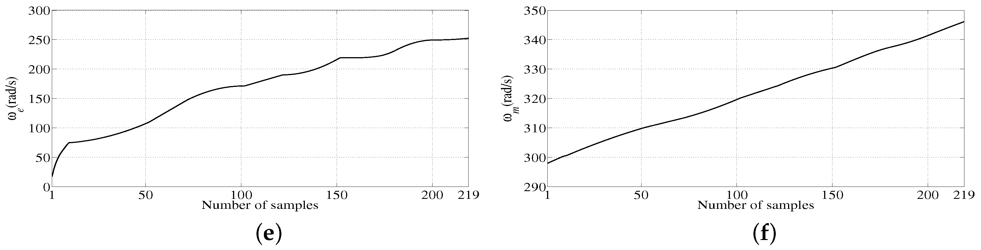
As shown in Figure 2a–c, the input data , and , which can fully excite the system characteristics of the HEV powertrain, are constructed. The system output and constrained outputs , can be obtained after the input data act on the built HEV dynamics model, as shown in Figure 2d–f. The sample time is chosen to be 0.01 s; the number of rows i in the input-output data matrix is chosen to be 20; and the number of columns j in the input-output data matrix is chosen to be 180. Thus, the open-loop data at 219 sampling instants are collected during the studied mode transition dynamic process.
Based on the sampling data as shown in Figure 2, the data block Hankel matrices , , , , , of input , output and constrained output can be constructed. Then, the subspace matrices , , and can be solved using the corresponding formulas.
3.3. Verification of the Subspace Predictor Equation
The input-output sampling data from the 220th–599th sampling instant are used to verify the effectiveness of the identified subspace predictor equation (i.e., whether the identified subspace predictor equation can well reflect the HEV’s dynamic characteristics). The constructed fully-excited input data , , and the specific identification prediction effect are shown in Figure 3.
As shown in Figure 3d–f, the predictive output can fit the actual output very well when is not equal to zero. Since the data used to identify the predictive model do not include the case that is equal to zero, a small predictive error appears when is equal to zero. The subject investigated in this paper is the clutch slipping phase during which is not equal to zero, so the predictive error appearing in Figure 3 will not influence the design of the proposed data-driven predictive controller.
3.4. Description of the Optimization Problem
The control input sequence increment to be optimized at time k can be expressed as follows:
where:
The predictive control output sequence is defined as follows:
and are used to represent the prediction horizon and the control horizon, respectively.
The cost function is usually defined as a quadratic form in order to make the predictive output as close as possible to a given reference output. A penalty term is added to the cost function to punish the violent changes of control variables. Therefore, considering the input and output constraints, the optimal control problem during the mode transition dynamic process from motor-only mode to compound driving mode can be described as below:
where:
In this cost function, the control objective of the first part is to force the clutch slip speed to converge to zero, which realizes the fast mode transition and reduces the wear and tear to the clutch. The control objective of the second part is to limit the torque changing rate of the engine, the clutch and the motor to ensure the mode transition comfortability. Obviously, these two control objectives are contradictory. The weighting factors and are given to trade off the two conflicting objectives. The bigger the weighting factor , the faster the mode transition process. The larger the weighting factor , the less the vehicle jerk.
is the reference sequence of within the prediction horizon, and is an adjustable parameter. The smaller is, the faster the clutch slip speed reaches zero. Thus, the clutch can finish the engagement more quickly.
3.5. Predictive Output Equation
In order to deal with the optimal control problem (19.a), the predictive output equation will be deduced in this section based on the data-driven method and the predictive control method.
To guarantee regulation with zero steady-state error for the reference input, the subspace matrix incremental input-output expressions are as follows:
and:
where:
Therefore, the optimal prediction of the future outputs can be derived as the following form:
where is the dynamic matrix containing the step response coefficients and formed from :
is constructed from , and is the free response for the case of measured disturbances:
, , , about can be calculated in the same way as (23)–(26).
3.6. Data-Driven Predictive Controller with Constraints
The DDPC problem (19.a) is usually converted into the following quadratic programming problem:
First, the expression of H and G will be briefly inferred. When (21) is substituted into (19.a), the following formula can be obtained:
where .
The last term in J is irrelevant to , so the cost function will be minimized if obtains the minimum.
where:
Therefore, the optimal problem (19.a) is converted into the quadratic programming problem (27).
Then, the constraint condition matrix and b of the quadratic programming problem (27) will be inferred from (19.b)–(19.d).
Let:
the constraint conditions (19.b)–(19.d) change to the following form:
For the constraint condition (31.a),
where:
Therefore, (31.a) can be changed to the following form:
Constraint Condition (31.b) can be changed to the following form:
Constraint Condition (31.c) can be changed to the following form from (22) and (30):
Overall, the constraint condition matrices can be derived as the following form:
According to the receding horizon principle of predictive control, only the first element of is implemented, and the calculation is repeated at each time instant. Hence, at the k-th sampling instant, the control law is given as follows:
4. Results and Discussion
The co-simulation of Cruise and MATLAB/Simulink R2010a is conducted under the urban driving cycle (UDC), which is shown in Figure 4a. The simulation time step is equal to 0.01 s. The maximum torque and maximum speed of the engine, clutch and motor are shown in Table 1. is chosen to be 20, and is chosen to be five. rad/s; r/min; r/min; ; ; and . To improve the transition comfortability, the variation ranges of control increments are as follows: Nm/s 50 Nm/s, Nm/s 50 Nm/s and Nm/s 100 Nm/s.
4.1. Data-Driven Predictive Control Method
Figure 4b–f show the Cruise simulation results of the proposed data-driven predictive torque coordination control strategy considering the constraints. At 60.44 s, the vehicle speed reaches 27 km/h; the mode transition from motor-only mode to parallel hybrid operation begins; the engine is started with a constant torque 60 Nm; and the two sides of the clutch are still separated. At 61.22 s, the engine speed rises very close to the motor speed (the clutch slip speed reaches 30 rad/s), and the clutch enters into the slipping phase. At about 61.49 s, the clutch slip speed reaches zero, then the clutch torque increases with a predetermined pattern to lock up reliably according to its characteristics. It can be seen that good transition quality can be achieved. The amplitude of vehicle jerk is 9.96 m/s, which avoids the discomfort of the passengers during the mode transition process. The mode transition duration is about 1.06 s, which can well meet the driver’s transition demand. The slipping duration of the clutch is only 0.27 s, and the total friction work is only about 8.59 J. This helps to prolong the clutch life.
The control effect of different switch triggers on the vehicle jerk, mode transition duration, clutch slipping duration and clutch frictional losses is shown in Table 2. Additionally, the vehicle jerk of the DDPC method under different is shown in Figure 5. It can be seen that a small switch trigger implies less usage of clutch torque. The smaller the switch trigger, the smaller the vehicle jerk and the less the clutch frictional losses. However, the smaller the switch trigger, the longer the mode transition duration. Taking sensor inaccuracy and actuator delay into account, it is hard to achieve small jerk with a too small [12], so is selected to be 30 rad/s.
4.2. Comparison with the Model Predictive Control Method
In this subsection, the torque coordination control effect of the DDPC method is compared with that of the MPC method to further illustrate the advantages of the proposed mode transition strategy.
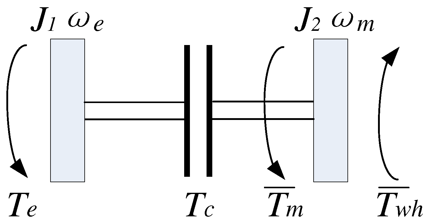
To get the model predictive torque coordination controller, the built HEV vehicle model as shown in Figure 1 can be simplified to the structure in Figure 6.
The equivalent inertia moment of the clutch input side , where is the inertia moment of the engine.
The equivalent inertia moment of the clutch output side can be expressed as:
where , , , and are the inertia moments of the clutch, motor, gearbox, single ratio transmission (SRT) and differential, respectively.
The vehicle resistance torque can be expressed as:
For the selected UDC, the road inclination angle is equal to zero; thus:
In the existing torque coordination control literature using the MPC method [10,11], for the convenience of the model predictive controller design, the contributions of the quadratic term of to are all considered small since the development of this powertrain model is built for the clutch engagement at low vehicle speeds (below 27 km/h). Thus, without significant loss of accuracy, the resistance torque is simplified as .
The equivalent vehicle resistance torque can be expressed as:
The state variable, control vector, output and constrained output are defined as:
Therefore, the dynamic equation in the mode transition of the HEV drive-line can be written as:
where:
Then, applying zero-order hold discretization with a sampling period to (32) gives the discrete state-space model:
where , .
The increment form of (33) is as follows:
The predictive output at the k-th instant is defined as:
The optimal control input sequence is defined as:
where:
The iteration form of (34) is:
where:
The cost function of the model predictive controller is selected the same as that of the data-driven predictive controller, which is shown in (19.a). The constrained model predictive control law can also be solved as a quadratic programming problem, where , .
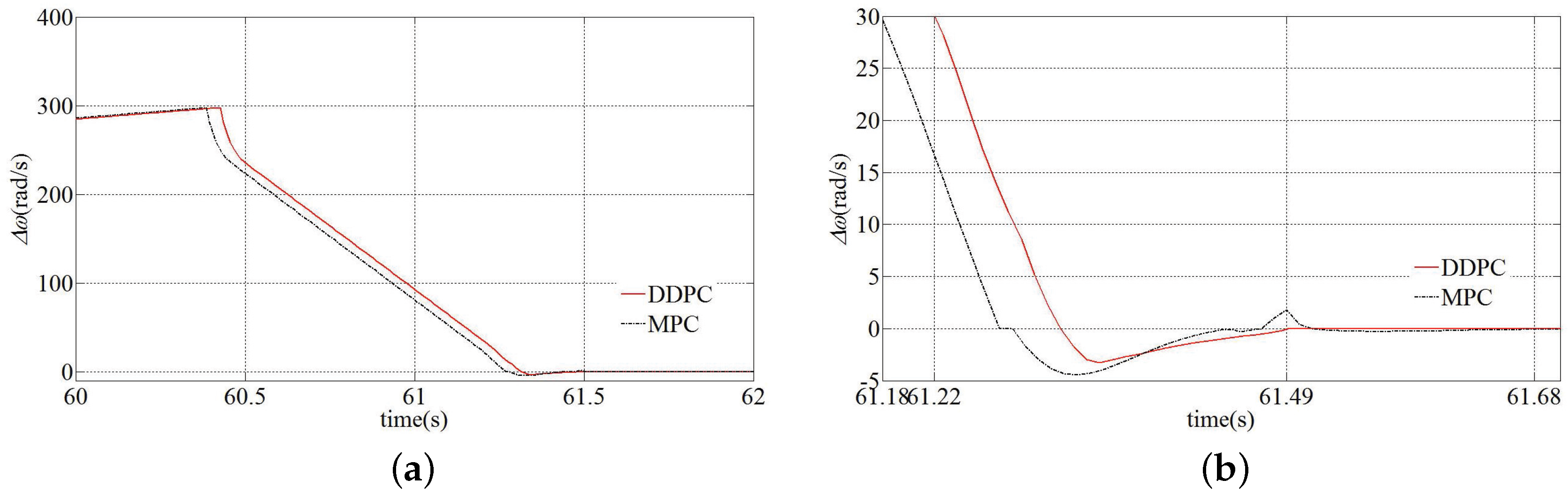
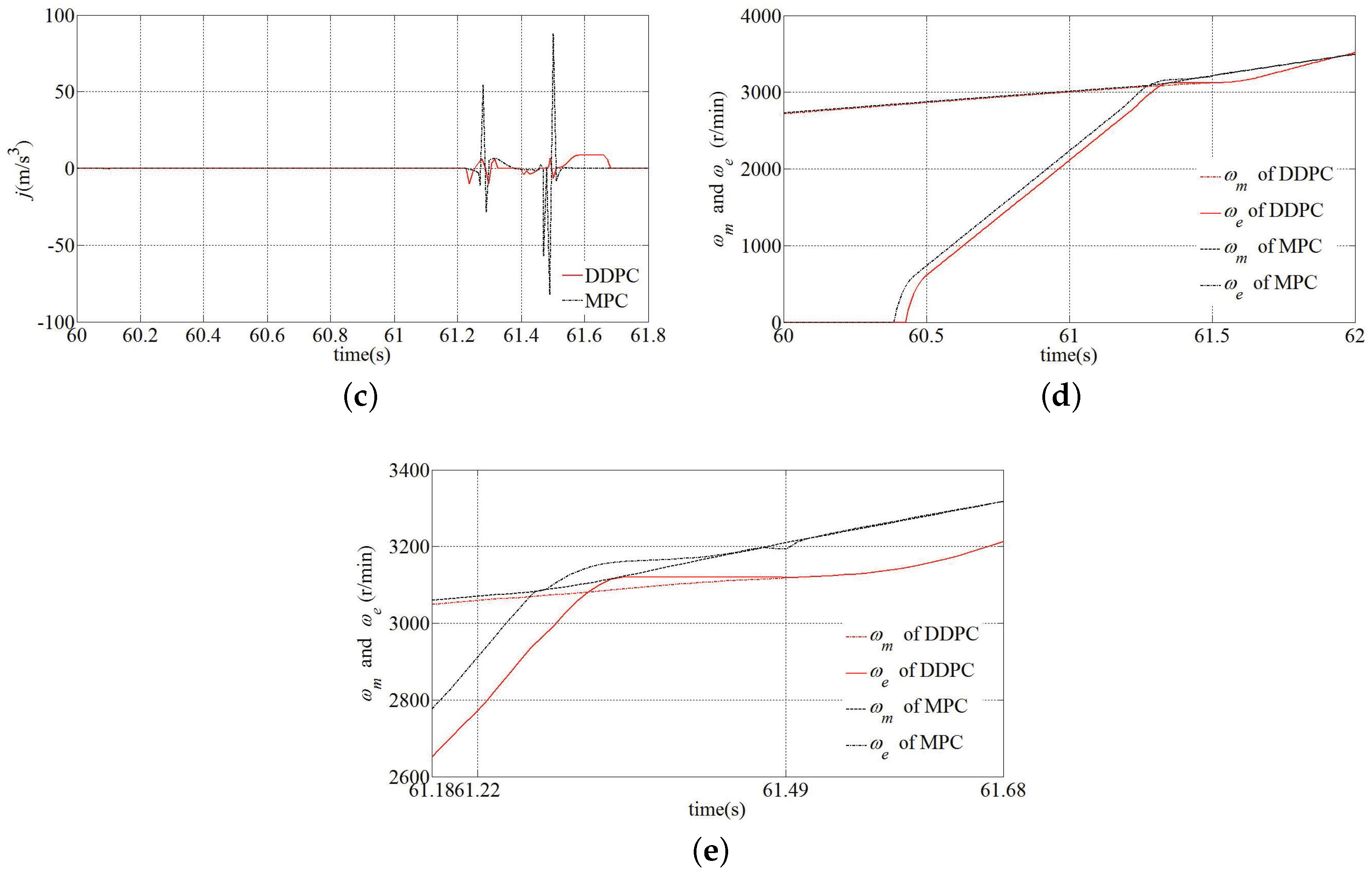
The results of the proposed DDPC method and the traditional MPC method are shown in Figure 7. To visually demonstrate the advantages of DDPC, the detailed data that can indicate the transition quality are shown in Table 3. As shown in the table, compared with the MPC method, the DDPC method can achieve smaller jerk, shorter mode transition duration, shorter clutch slipping duration and less clutch wear and tear under the same simulation conditions.
5. Conclusions
A new torque coordination control strategy based on the DDPC method has been proposed to solve the torque coordination problem during the HEV mode transition dynamic process to improve the mode transition quality. The conflicting control objectives of the mode transition, which are small jerk and short transition duration, have been simultaneously considered in the optimal objective function by tracking a properly-selected output reference sequence and limiting the change rates of the actuators. Cruise simulation results have validated the effectiveness of the proposed DDPC method. The results compared with the MPC have further shown that the DDPC can achieve higher mode transition quality, which contributes to the improvement of the riding comfortability and the economy of HEV greatly.
In this paper, the mode transition dynamic process from the motor-only mode to the compound driving mode has been taken as an example of the proposed DDPC method. As time goes on, the system characteristics and the component parameters may change with the long-term aging and the diverse driving conditions, so the predictive model should be updated using the real vehicle operation data, which are newly collected online so that the performance of the proposed strategy can be guaranteed steadily in the long term. The performance monitoring method of the data-driven predictive controller will be our future work.
Acknowledgments
This work was supported by the National Natural Science Foundation of China (Grant Numbers 61403236, 51277116, 61304130, 61304033 and 61573218) and the Doctoral Scientific Research Foundation of Shandong Technology and Business University (Grant Number BS201511).
Author Contributions
Jing Sun carried out the main research tasks and wrote the full manuscript. Guojing Xing provided important suggestions on the writing of the paper. Chenghui Zhang polished the paper.
Conflicts of Interest
The authors declare no conflicts of interest.
References
- Cairano, S.D.; Bernardini, D.; Bemporad, A.; Kolmanovsky, I.V. Stochastic MPC with learning for driver-predictive vehicle control and its application to HEV energy management. IEEE Trans. Control Syst. Technol. 2014, 3, 1018–1031. [Google Scholar] [CrossRef]
- Larsson, V.; Johannesson, L.; Egardt, B. Analytic solutions to the dynamic programming sub-problem in hybrid vehicle energy management. IEEE Trans. Veh. Technol. 2015, 4, 1458–1467. [Google Scholar] [CrossRef]
- Chen, Z.Y.; Xiong, R.; Wang, K.Y.; Jiao, B. Optimal energy management strategy of a plug-in hybrid electric vehicle based on a particle swarm optimization algorithm. Energies 2015, 8, 3661–3678. [Google Scholar] [CrossRef]
- Tong, Y. Real-time simulation and research on control algorithm of parallel hybrid electric vehicle. Chin. J. Mech. Eng. 2003, 10, 156–161. [Google Scholar] [CrossRef]
- Davis, R.I.; Lorenz, R.D. Engine torque ripple cancellation with an integrated starter alternator in a hybrid electric vehicle: Implementation and control. IEEE Trans. Ind. Appl. 2003, 6, 1765–1774. [Google Scholar] [CrossRef]
- Li, M.H.; Luo, Y.G.; Yang, D.G.; Li, K.Q.; Lian, X.M. A dynamic coordinated control method for parallel hybrid electric vehicle based on model matching control. Automot. Eng. 2007, 3, 203–207. [Google Scholar]
- Chiang, C.J.; Chen, Y.C.; Lin, C.Y. Fuzzy sliding mode control for smooth mode changes of a parallel hybrid electric vehicle. In Proceedings of the 2014 IEEE 11th International Conference on Control and Automation, Taichung, Taiwan, 18–20 June 2014; pp. 1072–1077. [Google Scholar]
- Koprubasi, K.; Westervelt, E.R.; Rizzoni, G. Toward the systematic design of controllers for smooth hybrid electric vehicle mode changes. In Proceedings of the 2007 American Control Conference, New York, NY, USA, 11–13 July 2007; pp. 2985–2990. [Google Scholar]
- Minh, V.T.; Rashid, A.A. Modeling and model predictive control for hybrid electric vehicles. Int. J. Autom. Technol. 2012, 3, 477–485. [Google Scholar] [CrossRef]
- Beck, R.; Saenger, S.; Richert, F.; Bollig, A.; Scholt, T.; Noreikat, K.E.; Abel, D. Model predictive control of a parallel hybrid vehicle drivetrain. In Proceedings of the 2005 44th IEEE Conference on Decision and Control, and the European Control Conference, Seville, Spain, 12–15 December 2005; pp. 2670–2675. [Google Scholar]
- Chen, L. Torque coordination control during mode transition for a series-parallel hybrid electric vehicle. IEEE Trans. Veh. Technol. 2012, 7, 2936–2949. [Google Scholar] [CrossRef]
- Sun, J.; Xing, G.J.; Liu, X.D.; Fu, X.L.; Zhang, C.H. A novel torque coordination control strategy of a single- shaft parallel hybrid electric vehicle based on model predictive control. Math. Probl. Eng. 2015, 1, 1–12. [Google Scholar] [CrossRef]
- Guo, L.; Ge, A.; Zhang, T.; Yue, Y. AMT shift process control. Trans. Chin. Soc. Agric. Mach. 2003, 2, 1–3. [Google Scholar]
- Xiong, R.; Sun, F.C.; Chen, Z.; He, H.W. A data-driven multi-scale extended Kalman filtering based parameter and state estimation approach of lithium-ion polymer battery in electric vehicles. Appl. Energy 2014, 1, 463–476. [Google Scholar] [CrossRef]
- Sun, F.C.; Xiong, R.; He, H.W. A systematic state-of-charge estimation framework for multi-cell battery pack in electric vehicles using bias correction technique. Appl. Energy 2016, 1, 1399–1409. [Google Scholar] [CrossRef]
- Kadali, R.; Huang, B.; Rossiter, A. A data driven subspace approach to predictive controller design. Control Eng. Pract. 2003, 3, 261–278. [Google Scholar] [CrossRef]
- Favoreel, W.; Moor, B.D. SPC: Subspace predictive control. In Proceedings of the 1999 14th World Congress, Beijing, China, 5–9 July 1999; pp. 1–11. [Google Scholar]
- Gao, C.H.; Jian, L.; Liu, X.Y.; Chen, J.M.; Sun, Y.X. Data-driven modeling based on volterra series for multidimensional blast furnace system. IEEE Trans. Neural Netw. 2011, 12, 2272–2283. [Google Scholar]
- Kusiak, A.; Song, Z.; Zheng, H.Y. Anticipatory control of wind turbines with data-driven predictive models. IEEE Trans. Energy Convers. 2009, 3, 766–774. [Google Scholar] [CrossRef]
- Gil, P.; Henriques, J.; Cardoso, A.; Carvalho, P.; Dourado, A. Affine neural network-based predictive control applied to a distributed solar collector field. IEEE Trans. Control Syst. Technol. 2014, 2, 585–596. [Google Scholar] [CrossRef]
- Ge, S.S.; Li, Z.J.; Yang, H.Y. Data driven adaptive predictive control for holonomic constrained under-actuated biped robots. IEEE Trans. Control Syst. Technol. 2012, 3, 787–795. [Google Scholar] [CrossRef]
- Wahab, N.A.; Katebi, R.; Balderud, J.; Rahmat, M.F. Data-driven adaptive model-based predictive control with application in wastewater systems. IET Control Theory Appl. 2011, 6, 803–812. [Google Scholar] [CrossRef]
- Yin, X.H.; Li, S.Y.; Wu, J.; Li, N.; Cai, W.J.; Li, K. Data-driven based predictive controller design for vapor compression refrigeration cycle systems. In Proceedings of the 2013 9th Asian Control Conference, Istanbul, Turkey, 23–26 June 2013; pp. 1–6. [Google Scholar]
- Lu, X.H.; Chen, H.; Wang, P.; Gao, B.Z. Design of a data-driven predictive controller for start-up process of AMT vehicles. IEEE Trans. Neural Netw. 2011, 12, 2201–2212. [Google Scholar]
- Lu, X.H.; Chen, H.; Gao, B.Z.; Zhang, Z.W.; Jin, W.W. Data-driven predictive gearshift control for dual-clutch transmissions and FPGA implementation. IEEE Trans. Ind. Electron. 2015, 1, 599–610. [Google Scholar] [CrossRef]
- Zhong, L.S.; Yan, Z.; Yang, H.; Qi, Y.P.; Zhang, K.P.; Fan, X.P. Predictive control of high-speed train based on data driven subspace approach. J. China Railw. Soc. 2013, 4, 77–83. [Google Scholar]
Figure 1.
The block diagram of the powertrain configuration.
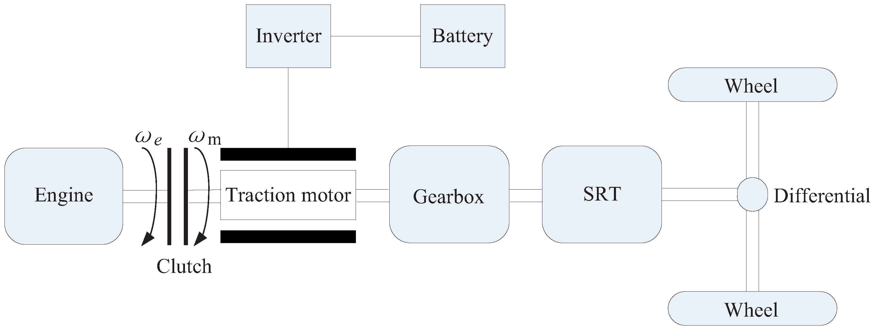
Figure 2.
Input and output data of 219 sample points for identification: (a) Engine torque ; (b) Clutch torque ; (c) Motor torque ; (d) The clutch slip speed ; (e) Engine speed ; (f) Motor speed .
Figure 2.
Input and output data of 219 sample points for identification: (a) Engine torque ; (b) Clutch torque ; (c) Motor torque ; (d) The clutch slip speed ; (e) Engine speed ; (f) Motor speed .
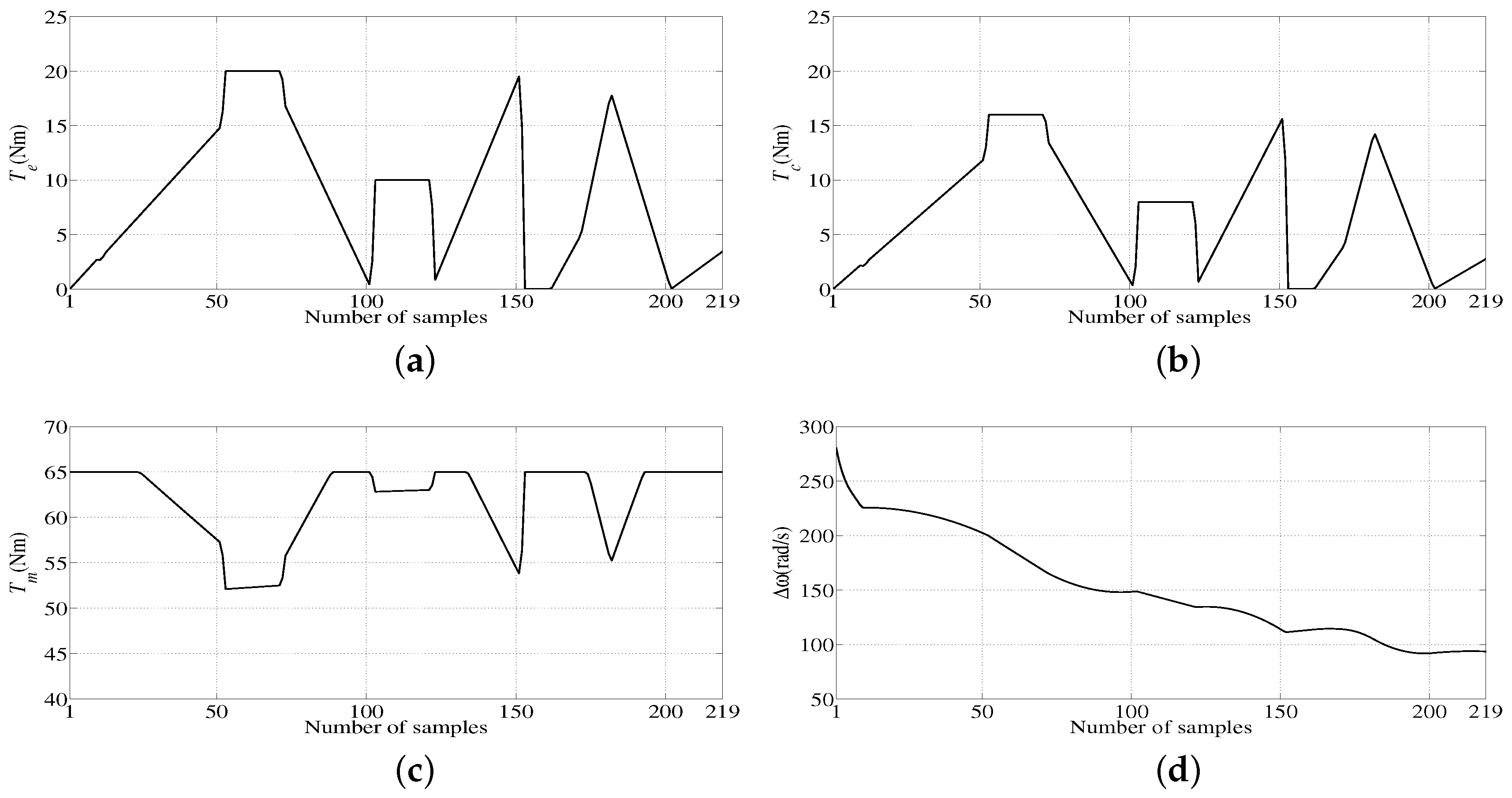

Figure 3.
Input and output data for verification and identification results: (a) Engine torque ; (b) Clutch torque ; (c) Motor torque ; (d) The identified results of the clutch slip speed ; (e) The identified results of constrained engine speed ; (f) The identified results of constrained motor speed .

Figure 4.
Cruise simulation results of the data-driven predictive controller considering the constraints: (a) Urban driving cycle (UDC); (b) Jerk; (c) The clutch slip speed ; (d) The engine torque ; (e) The clutch torque ; (f) The motor torque .
Figure 4.
Cruise simulation results of the data-driven predictive controller considering the constraints: (a) Urban driving cycle (UDC); (b) Jerk; (c) The clutch slip speed ; (d) The engine torque ; (e) The clutch torque ; (f) The motor torque .
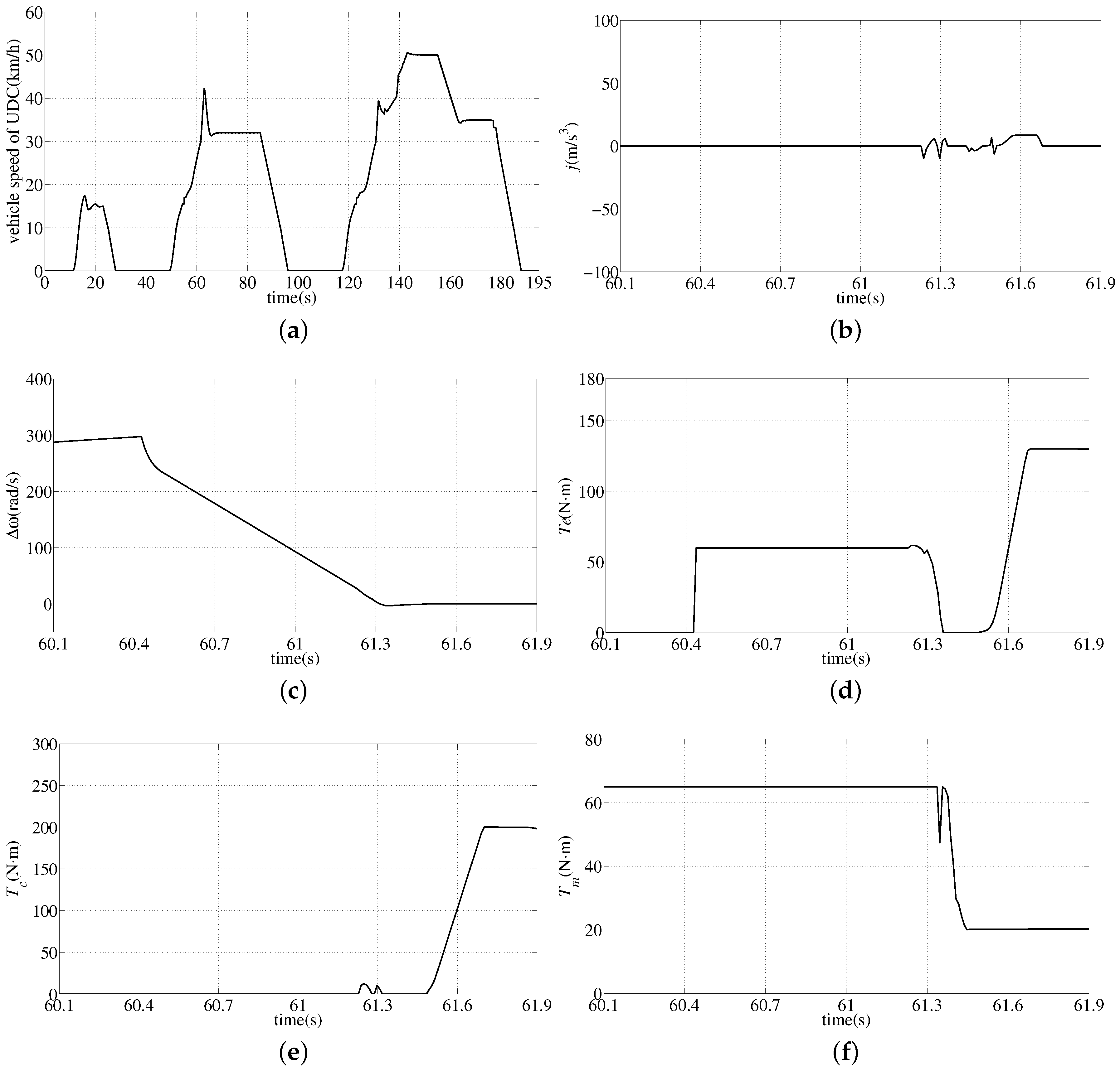
Figure 5.
Vehicle jerk of data-driven predictive controller considering the constraints under different .
Figure 5.
Vehicle jerk of data-driven predictive controller considering the constraints under different .
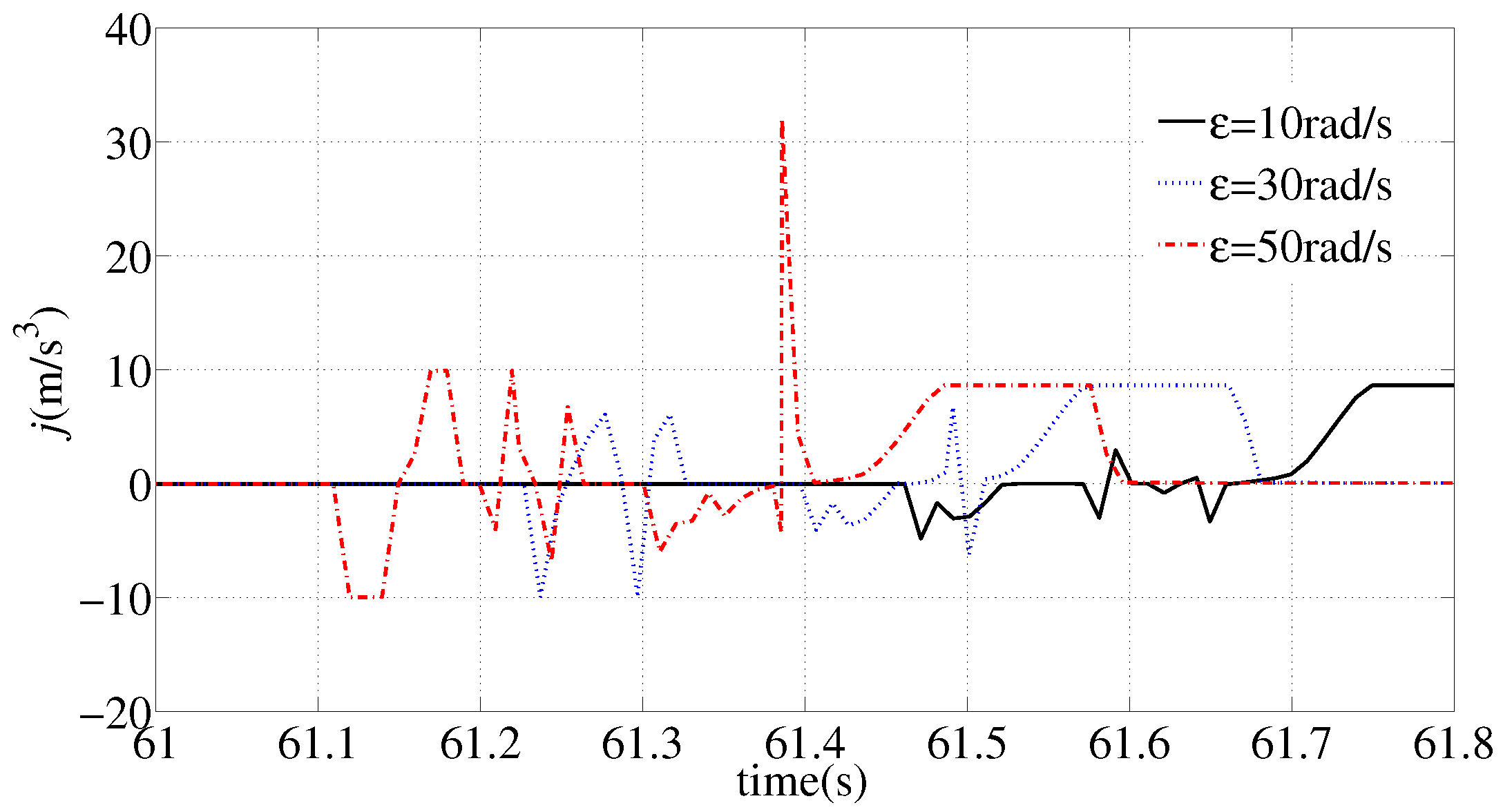
Figure 6.
Simplified model of the HEV drive-line.

Figure 7.
Comparison between the DDPC method and the MPC method for the torque coordination control problem during the mode transition dynamic process from the motor-only mode to compound driving mode: (a) The clutch slip speed ; (b) Partially enlarged view of (a); (c) Jerk; (d) The motor speed and the engine speed ; (e) Partially enlarged view of (d).


Table 1.
Key vehicle parameters in the cruise simulation platform.
| Component | Parameter | Value and Unit |
|---|---|---|
| Vehicle | Vehicle mass | 1430 kg |
| Air density | 1.29 kg/m | |
| Vehicle frontal area | 2.15 m | |
| Aerodynamic drag coefficient | 0.3 | |
| Engine | Moment of inertia | 0.19 kg·m |
| Maximum speed | 5800 r/min | |
| Maximum torque | 130 Nm | |
| Clutch | Moment of inertia | 0.001 kg·m |
| Maximum transferable torque | 200 Nm | |
| Motor | Moment of inertia | 0.15kg·m |
| Maximum speed | 8000 r/min | |
| Maximum torque | 65 Nm | |
| Battery | Maximum charge | 50 Ah |
| Tyre | Moment of inertia | 1.1 kg·m |
| Dynamic rolling radius | 0.308 m | |
| Gear Box | Moment of inertia | 0.005 kg·m |
| Gear ratio | 3.62, 2.22, 1.51, 1.08, 0.85 | |
| SRT | Moment of inertia | 0.018 kg·m |
| Transmission ratio | 5.5 | |
| Differential | Torque split factor | 1.0 |
| Moment of inertia | 0.02 kg·m |
Table 2.
Cruise simulation results of data-driven predictive controller under different speed difference thresholds.
Table 2.
Cruise simulation results of data-driven predictive controller under different speed difference thresholds.
| Jerk Range | Transition Duration | Clutch Slipping Duration | Clutch Frictional Losses | |
|---|---|---|---|---|
| 10 rad/s | −4.8–2.96 m/s | 1.18 s | 0.32 s | 0.002 J |
| 30 rad/s | −9.96–6.76 m/s | 1.06 s | 0.29 s | 8.59 J |
| 50 rad/s | −9.96–32.1 m/s | 1.01 s | 0.27 s | 42.92 J |
Table 3.
Cruise simulation results compare between the DDPC method and the MPC method.
| Indices | DDPC | MPC |
|---|---|---|
| Jerk Fluctuation Range | −9.96–6.76 m/s | −82.47–87.92 m/s |
| Mode Transition Duration | 1.05 s | 1.24 s |
| Clutch Slipping Duration | 0.27 s | 0.5 s |
| Clutch Frictional Losses | 8.59 J | 19.3 J |
© 2017 by the authors. Licensee MDPI, Basel, Switzerland. This article is an open access article distributed under the terms and conditions of the Creative Commons Attribution (CC BY) license (http://creativecommons.org/licenses/by/4.0/).
Share and Cite
MDPI and ACS Style
Sun, J.; Xing, G.; Zhang, C. Data-Driven Predictive Torque Coordination Control during Mode Transition Process of Hybrid Electric Vehicles. Energies 2017, 10, 441. https://doi.org/10.3390/en10040441
AMA Style
Sun J, Xing G, Zhang C. Data-Driven Predictive Torque Coordination Control during Mode Transition Process of Hybrid Electric Vehicles. Energies. 2017; 10(4):441. https://doi.org/10.3390/en10040441
Chicago/Turabian StyleSun, Jing, Guojing Xing, and Chenghui Zhang. 2017. "Data-Driven Predictive Torque Coordination Control during Mode Transition Process of Hybrid Electric Vehicles" Energies 10, no. 4: 441. https://doi.org/10.3390/en10040441
Note that from the first issue of 2016, this journal uses article numbers instead of page numbers. See further details here.