A Time-Efficient Approach for Modelling and Simulation of Aggregated Multiple Photovoltaic Microinverters

Abstract

This paper presents a time-efficient modeling and simulation strategy for aggregated microinverters in large-scale photovoltaic systems. As photovoltaic microinverter systems are typically comprised of multiple power electronic converters, a suitable modeling and simulation strategy that can be used for rapid prototyping is required. Dynamic models incorporating switching action may induce significant computational burdens and long simulation durations. This paper introduces a single-matrix-form approach using the average model of a basic microinverter with two power stages consisting of a dc-dc and dc-ac converter. The proposed methodology using a common or intermediate source between two average models of cascaded converters to find the overall average model is introduced and is applicable to many other converter topologies and combinations. It provides better flexibility and simplicity when investigating various power topologies in system-level studies of microinverter and other power electronic systems. A 200 W prototype microinverter is tested to verify the proposed average and dynamic models. Furthermore, MATLAB/Simulink (2010a, Mathworks, Natick, MA, USA) is used to show the improved simulation speed and maintained accuracy of the multiple microinverter configurations when the derived average model is compared to a dynamic switching simulation model.

1. Introduction

Photovoltaic (PV) power is becoming more prevalent as its cost has become more competitive with traditional power sources and it is especially attractive for microgrids. As PV systems become more popular, higher efficiency and reliability are of increasing importance. Researchers have developed many effective designs and methodologies that address several essential aspects to improve the performance of PV systems. Modified or optimized power electronic energy conversion topologies have gained significant interest since power stage configuration has significant impact on the system: For example, recent work has shown that microinverters can yield significant reliability enhancement in PV systems [1]. Another example is shown in [2] where different targets, such as efficiency, reliability and cost, were considered to optimize the design of synchronous rectification (SR) boost topology. A third example is a new cascaded active-front-end converter is proposed in [3] to increase system reliability and decrease cost. A single-stage PV system [4] and a modified dual-stage inverter [5] along with maximum power point tracking (MPPT), grid synchronization, and harmonic reduction, have been implemented. Among all these designs, selecting proper converter topologies and components and evaluating their performance, system modelling is critical to address higher efficiency and reliability needs [6,7]. Advanced control has also been of interest enhance maximum power point tracking (MPPT) in PV systems [8,9,10]. For example, recent work shown in [11] focused on distributed maximum power point tracking (DMPPT) converter design methodology to deal with the problem of variation in temperature, irradiance and shadowing. Other efficiency and power quality enhancement methods include those that utilize an energy storage device [12] or shunt active power filter [13] on the bases of conventional inverter operation. PV systems can be classified per their connection method between the PV modules and the power conditioning system (PCS). In a conventional string configuration, shown in Figure 1a, which can also be connected with several parallel strings, several series PV modules deliver electrical power to the grid and local ac loads through a central PCS. An example is Nano Grid integration [14], which utilizes a central PCS to control multiple of small distributed generation clusters. However, the central PCS configuration may cause mismatch losses of arrays due to differences in manufacturing, temperature, shading, and degradation conditions among the PV modules, resulting in a less efficient PV system. Also, failure of the PCS affects the reliability of the whole system. On the other hand, the microinverter configuration shown in Figure 1b, also referred to as the module-integrated converter (MIC), uses individual small PCSs mounted on each PV module, allowing a simple “plug and play” installation and more localized control such as independent maximum power point tracking (MPPT) at the individual PV module scale [15,16,17,18]. Compared to the centralized PCS configuration, this system is expected to be more reliable with higher energy yield, which justifies its minor cost increase. Comparison based on experimental testing of PCSs is provided in [19], but due to the variations of operating conditions, experimental testing is not convenient or cost effective for one-to-one comparisons between various PCSs and under different conditions.

Modeling and simulation has thus become essential especially in order to choose the proper topology, select appropriate circuit component types and values, evaluate circuit performance, and complete a system design [20,21]. There are several methods to build power electronics models and they usually involve switching power devices and passive power elements such as inductors, capacitors, and resistors. Dynamic models have been used to analyze the performance of an inverter [5], but dynamic models including switching actions may not be suitable for multiple-microinverter aggregated system simulations despite their simple implementation and accurate transient responses. The increase in the number of microinverters in a system simulation yields significant computational burdens and long simulation times [22]. Another approach is to use the average pulse width modulation (PWM) switch model replacing the switches in the dynamic models with time-averaged models represented by voltage and current sources [23]. With the average modeling method, some simulation accuracy is lost but the resulting simulation run time and setup time can be significantly reduced. The state-space average model is employed to ascertain a set of equations describing the system behavior over one switching period, which aids designers in understanding the physical relationship between control parameters and converter states [20]. Using an average model, the transfer function of the system can also be obtained, and larger simulation step sizes can be utilized with minimal loss of accuracy which leads to a faster simulation time. Consequently the state-space average model will be the most competitive modeling method in simulation studies for aggregated multiple microinverters.

A number of papers have examined the state-space averaging model for various power converter topologies in different operating modes [24,25,26,27,28,29,30,31,32,33]. The proper analytical averaging model for discontinuous conduction mode (DCM) operation in the dc-dc converter has been studied in [24], which contains implicitly elements to generate a base model applicable to both fixed and variable frequency operations. Many efforts have also been made to develop adequate seamless mode transitions from DCM to continuous conduction mode (CCM) and vice versa in simulation studies of dc-dc converters [25,26]. Furthermore, the issue of parasitic components on these modeling methods is investigated in [27]. Recently the conventional converter configurations such as the boost, buck and fly-back converter tend to be combined and integrated with other power electronics circuits for high efficiency converters and thus their proper averaging model have been required. The boost converter with a voltage multiplier cell has been analyzed in [28] to derive its average model which is complex and requires the use of advanced techniques due to the resonant circuit. Not only small-signal model approaches, but also large-signal model approaches have been conducted to investigate large signal behaviors and capabilities in multiple dc-dc [29] or dc-ac [30] converters where a generalized state-space averaging method employing the Fourier series with time-dependent coefficients. However, these models cannot predict the complete dynamic behavior of these systems. While most papers focus on dc-dc converter modeling, a small number of papers have been presented on average modeling of dc-ac converters to approximate their behavior in grid-connected power electronics such as static synchronous compensators (STATCOM), active power filters [31] and PV applications [32]. It should be noted that references [24,25,26,27,28,29,30,31,32,33] have all addressed single-stage power converters and inverters, but average modeling of multiple-stage converters such as microinverters is still open to research along with the adequate simulation strategy that is necessary to improve simulation speed and accuracy of multiple cascaded converters, such as multiple PV microinverters in a microgrid.

The primary objectives of this paper are to introduce the simulation strategy for aggregated multiple microinverters by employing state-space average modeling of multi-stage power converters represented by a single-matrix-form (SMF). SMF can be derived by using the intermediate source model to link to converters with established average models, and thus this approach can facilitate integration of existing average models for cascaded, parallel, and many topologies. Since the proposed simulation strategy is based on the state-space average modeling technique which allows investigating small-signal behavior of the systems, it can capture important dynamics of PV microinverters in smaller power systems such as microgrids even under aggregated multiple converters, but switching transients that slow down simulations are over-ridden. The main advantages of this proposed approach are: (1) achieving a faster simulation time in research on aggregated multiple microinverter systems compared to dynamic switching models of converters; (2) providing better flexibility with easily interchangeable converter models; (3) understanding the relationship of state variables between multi-stage converters; and (4) simple extension to other power electronics conversion systems with multiple-stage configurations. It is important to note that the main purpose of this paper is to introduce this intermediate source methodology in multiple-converter systems which can be extended to various topologies and applications, especially in the area of modeling and control of microgrids to capture finer dynamics with faster simulations that mask switching transients.

This paper starts with descriptions of the proposed simulation strategy and state-space average modeling of microinverters in Section 2. Model validation is carried out by comparing waveforms from simulation results in MATLAB/Simulink with experimental results from a 200 W prototype microinverter board in Section 3. These results are compared in open-loop mode to test the “plant” dynamics using the proposed model, dynamic simulation model, and experiments. The general control strategy for microinverters in PV applications is explained in Section 4, and then the simulation times between the proposed modeling approach and the dynamic model are compared in Section 5. Finally, Section 6 concludes the paper.

2. Proposed Simulation Strategy and State-Space Average Model with a Single Matrix-Form

It is common for PV microinverters to have multiple-stage configurations consisting of dc-dc and dc-ac stages [15,16,34]. The dc-dc converter provides MPPT at the PV panel terminals while the dc-ac converter delivers PV power to the grid or local ac loads in the second stage as shown in Figure 2. The proposed approach to simulate the multiple microinverter system is shown in Figure 3. Several models are required for a PV system simulation—PV module model, power converter model, grid model and local load model. PV cell models are very common in the literature, especially those utilizing the current source and inverse diode configuration [35]. Using this model, a 200 W PV panel model is developed under different irradiance conditions. As for the load model, a simple resistor model is used as the passive Local Load Model in Figure 3 since it yields simpler SMF. If reactive power needs to be consumed or generated by local loads, the resistive load model can be replaced with other inductive and capacitive loads or an RLC combination. The grid model encompasses a stiff single-phase voltage source with fixed voltage and frequency characteristics in series with the grid impedance consisting of a resistor and inductor. By using this model, it is possible to simulate all grid disturbances such as sag, swell, and interruptions, and adjust the voltage source to include voltage harmonics. Details of the converter dc-dc, dc-ac, and combined converter models are presented in this section.

While this paper presents examples of specific dc-dc and dc-ac stages, adjusting the matrices in the average model of each stage to reflect other converter topologies is possible. The methodology proposed in this paper for integrating two average models of dc-dc and dc-ac stages as shown in Figure 4 can thus be followed. A SMF integrated with the dc-dc converter and dc-ac converter models is used for better flexibility when other topologies are used as it directly links the state variables between both energy conversion stages.

2.1. DC-DC Converter Model

State-space average modeling is employed to obtain a set of differential equations applicable to a selected converter topology [20]. The resulting model is expected to combine the dc-dc converter in CCM and dc-ac converter. Those equations are capable of describing the system behavior over one switching period. It is also desirable to include all parasitic effects in the state-space average model to predict the dynamic behavior and frequency response of the microinverter accurately [27,36]. The state space equation of the converter in CCM can be expressed as:

$$\dot{x}(t)=\left(q(t){\mathbf{A}}_1+(1-q(t)){\mathbf{A}}_2\right)\mathbf{x}(t)+\left(q(t){\mathbf{B}}_1+(1-q(t)){\mathbf{B}}_2\right)\mathbf{u}(t)$$

(1)

where q(t) is the switching function corresponding to the power device’s on/off states, A_k and B_k are the system matrices where k = 1 or 2 depending on the switch status, and u(t) is the input vector. The low-frequency components of state variables such as the inductor currents, capacitor voltages and the output duty can be modeled by averaging over the switching period T_s and can be defined as:

$$\overline{x}(t)=\frac{1}{T_s}{\displaystyle {\int }_t^{t+T_s}\mathbf{x}(\tau )d}\tau$$

(2)

where the bar symbol denotes the so-called fast average or true average of a state variable x(t). Using (2), the state average equation can be expressed as:

$$\dot{\overline{x}}(t)=\left(d(t){\mathbf{A}}_1+(1-d(t)){\mathbf{A}}_2\right)\overline{x}(t)+\left(d(t){\mathbf{B}}_1+(1-d(t)){\mathbf{B}}_2\right)\overline{u}(t)$$

(3)

where d(t) is the duty cycle function.

As an example, Figure 5 depicts the grid-connected microinverter, consisting of a non-ideal boost converter and H-bridge inverter. To obtain the state-space average model with a SMF, these converters can be considered separately as shown in Figure 6 and Figure 7. The circuit equations of these converters for turn-on and turn-off periods can be derived by applying Kirchoff’s voltage and current laws, and then the system matrices according to the switching status can be obtained. From the dc-dc boost converter shown in Figure 6, the state-space average model can be defined as:

$$\begin{array}{cc}\hfill {\dot{\overline{x}}}_d(t)& ={\mathbf{A}}_d{\overline{x}}_d(t)+{\mathbf{B}}_d{\overline{u}}_d(t)\hfill \\ & =\left(D_{dc}(t){\mathbf{A}}_{d1}+(1-D_{dc}(t)){\mathbf{A}}_{d2}\right){\overline{x}}_d(t)\hfill \\ & +\left(D_{dc}(t){\mathbf{B}}_{d1}+(1-D_{dc}(t)){\mathbf{B}}_{d2}\right){\overline{u}}_d(t)\hfill \end{array}$$

(4)

where x_d = [i_pv v_Cdc]^T, u_d = [v_pv v_m v_d i_dc]^T and i_pv is the dc inductor current, v_Cdc is the link capacitor voltage, v_pv is the output voltage of the PV module, v_m is the drain-to-source voltage of the boost switch, v_d is the forward voltage of the diode, i_dc is the current in the dc-bus and D_dc is the duty ratio of the boost converter. Matrices A_d1, A_d2, B_d1 and B_d2 when the switch is on and off are presented in Appendix A. Using these matrices and (4), matrices A_d and B_d presented with averaged values during one-sample time are:

$${\mathbf{A}}_d=\left[\begin{array}{cc}-\frac{R_{Ldc}+D_{dc}{R}_{Mdc}+\left(R_{Cdc}+R_d\right)(1-D_{dc})}{L_{dc}}& -\frac{1-D_{dc}}{L_{dc}}\\ \frac{1-D_{dc}}{C_{dc}}& 0\end{array}\right]$$

(5)

$${\mathbf{B}}_d=\left[\begin{array}{cccc}\frac{1}{L_{dc}}& -\frac{D_{dc}}{L_{dc}}& -\frac{1-D_{dc}}{L_{dc}}& \frac{(1-D_{dc})R_{Cdc}}{L_{dc}}\\ 0& 0& 0& -\frac{1}{C_{dc}}\end{array}\right]$$

(6)

where L_dc is the boost inductor value, C_dc is the dc link capacitor value, R_Ldc and R_Cdc are the parasitic resistors of the passive and active components, R_Mdc and R_d are the switch on-resistance, respectively.

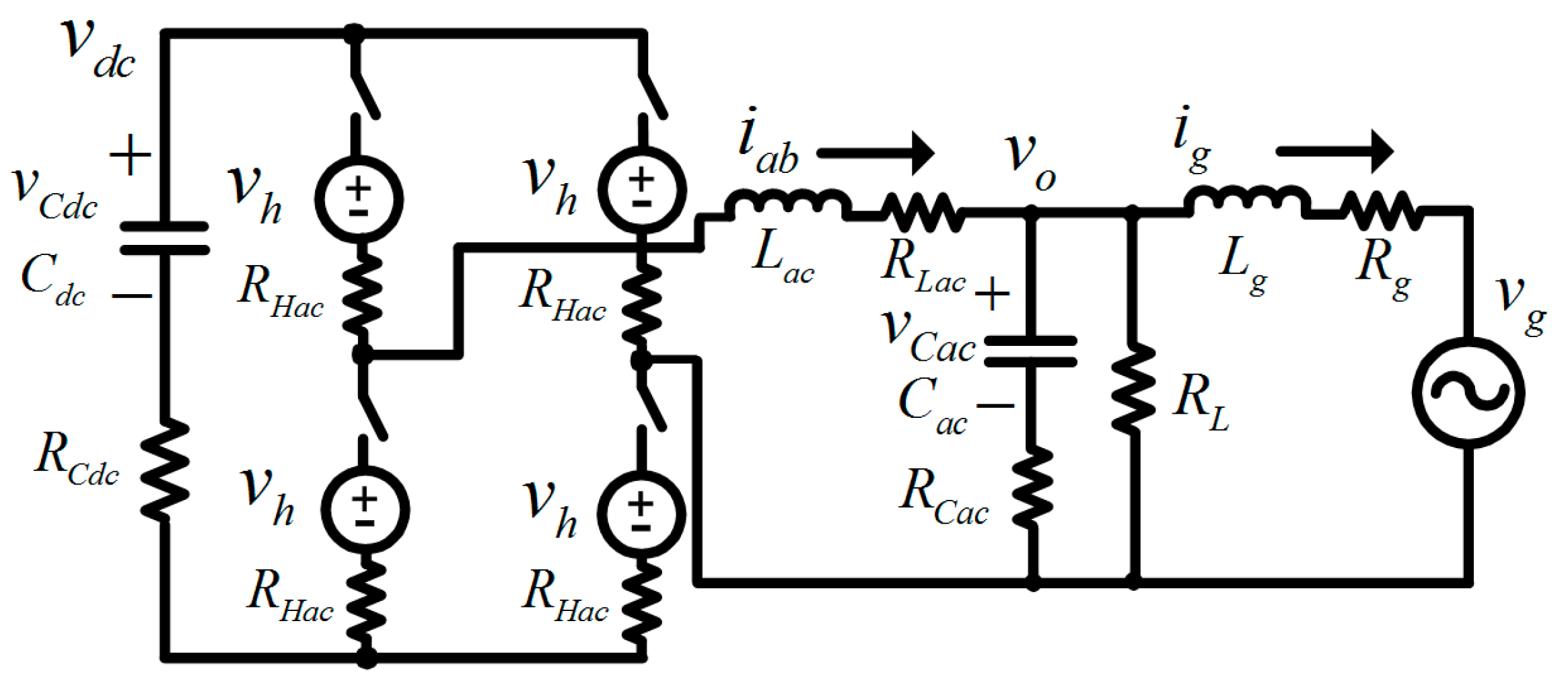
2.2. DC-AC Converter Model

In a procedure similar to that discussed in the previous section, the average model of the H-bridge converter shown in Figure 7 is defined as:

$$\begin{array}{l}{\dot{\overline{x}}}_a(t)={\mathbf{A}}_a{\overline{x}}_a(t)+{\mathbf{B}}_a{\overline{u}}_a(t)\\ =\left(D_{ac}(t){\mathbf{A}}_{a1}+(1-D_{ac}(t)){\mathbf{A}}_{a2}\right){\overline{x}}_a(t)\\ +\left(D_{ac}(t){\mathbf{B}}_{a1}+(1-D_{ac}(t)){\mathbf{B}}_{a2}\right){\overline{u}}_a(t)\end{array}$$

(7)

where x_a = [i_ab v_Cac i_g]^T, u_a = [v_Cdc v_h v_g]^T, i_ab is the ac inductor current, v_Cac is the capacitor voltage in the LC filter, i_g is the grid current, v_h is the drain-to-source voltage of the H-bridge switch, v_g is the grid voltage and D_ac is the duty ratio of the H-bridge converter.

It is worthwhile to mention that the relationship between the average duty and modulation index (M) of the H-bridge converter can be expressed as D_ac(t) = 0.5 + M∙sin(ωt) where ω is the grid frequency since the average duty is between 0 and 1. Matrices A_a1, A_a2, B_a1 and B_a2 are shown in the Appendix A. Using these matrices and (7), matrices A_a and B_a for averaged values during one-sample time are given by:

$${\mathbf{A}}_a=\left[\begin{array}{ccc}\frac{-\left(\begin{array}{l}2R_{Hac}+R_{Lac}\\ +R_{Cac}\Psi +R_{Cdc}\end{array}\right)}{L_{ac}}& -\frac{\Psi }{L_{ac}}& \frac{R_{Cac}\Psi }{L_{ac}}\\ \frac{\Psi }{C_{ac}}& -\frac{\Psi }{C_{ac}{R}_L}& -\frac{\Psi }{C_{ac}}\\ \frac{R_{Cac}\Psi }{L_g}& \frac{\Psi }{L_g}& -\frac{\Psi }{L_g}\left(\begin{array}{l}{R}_{Cac}+R_g\\ +\frac{R_{Cac}{R}_g}{R_L}\end{array}\right)\end{array}\right]$$

(8)

where $\Psi =\frac{R_L}{R_L+R_{Cac}}$, and:

$${\mathbf{B}}_a=\left[\begin{array}{ccc}\frac{(2D_{ac}-1)}{L_{ac}}& -\frac{2}{L_{ac}}& 0\\ 0& 0& 0\\ 0& 0& -\frac{1}{L_g}\end{array}\right]$$

(9)

where, L_ac is the ac inductor value, C_ac is the capacitor value in the LC filter, R_Lac and R_Cac, are the parasitic resistors of the passive components, R_L is the local load resistance, and L_g and R_g reflect the grid impedance, respectively.

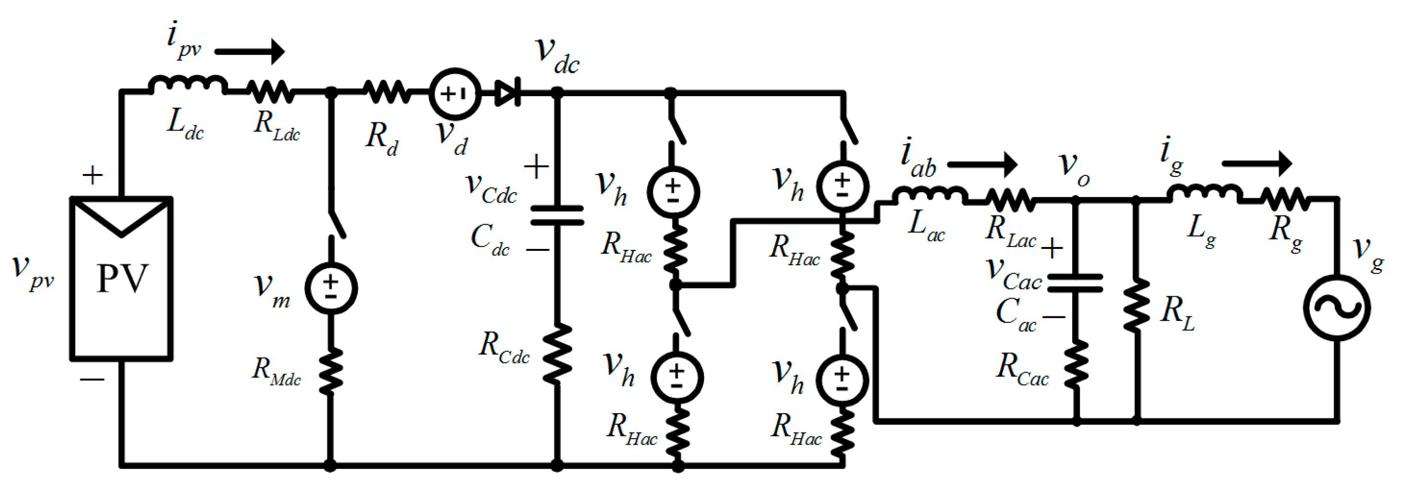
2.3. Combined Average Model

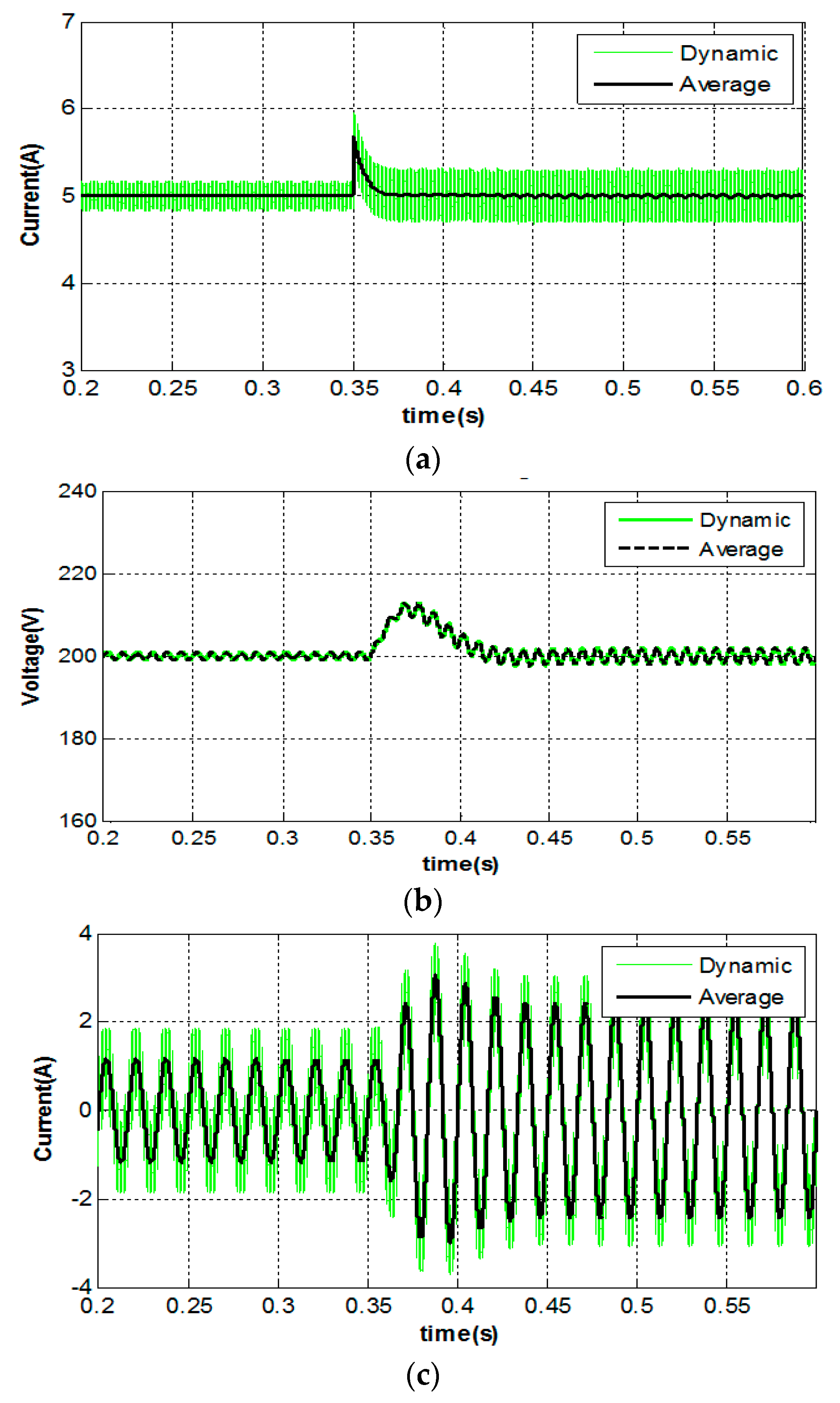
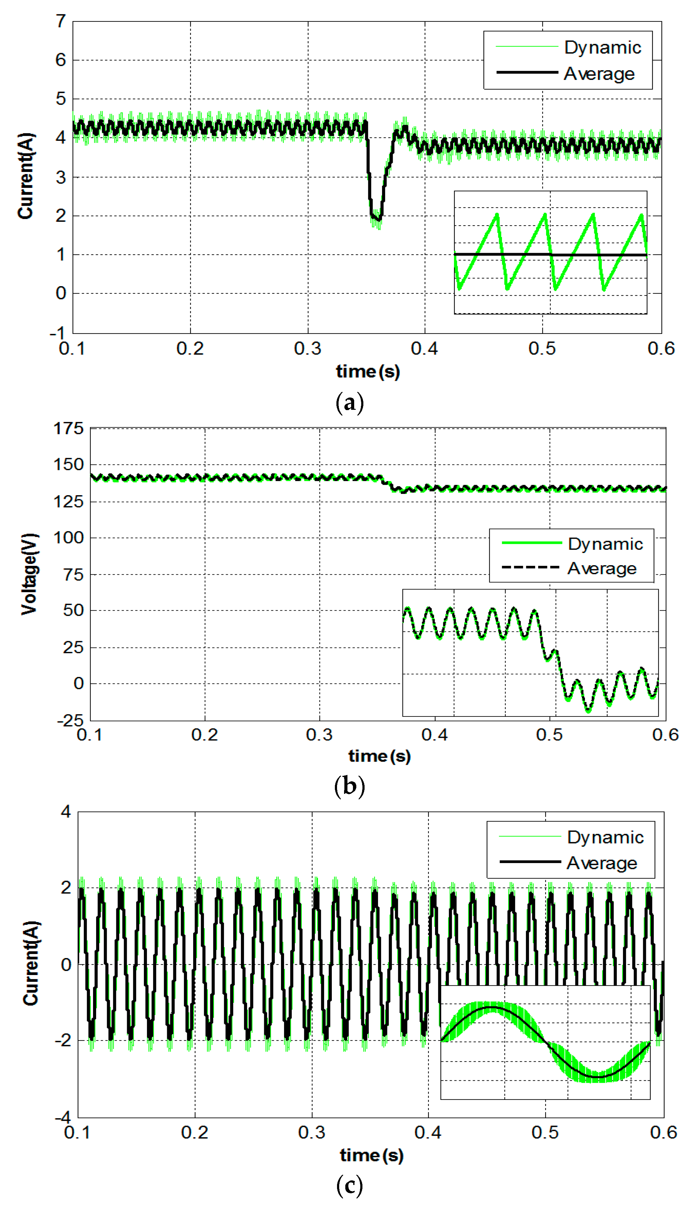
As the next step, using the relationship between the dc-bus current and output current, the two state-space average models obtained in (4) and (7) can be combined into SMF since the common source in the previously derived two state-space average model is the dc-bus current. Thus, the dc-bus current can be represented by ac current and ac duty in the H-bridge converter as:

$${\overline{i}}_{dc}=(2D_{ac}-1){\overline{i}}_{ab}$$

(10)

It is notable in (10) that the common source model causes the dc-bus current to include ac ripples that are twice the ac output frequency, which is also reflected to dc-bus voltage. Moreover, the dc voltage v_dc and the output ac voltage v_o can be expressed as:

$${\overline{v}}_{dc}=R_{Cdc}{\overline{i}}_{pv}+{\overline{v}}_{Cdc}-R_{Cdc}{\overline{i}}_{ab}$$

(11)

$${\overline{v}}_o=\left(\frac{R_L{R}_{Cac}}{R_L+R_{Cac}}\right){\overline{i}}_{ab}+\left(\frac{R_L}{R_L+R_{Cac}}\right){\overline{v}}_{Cac}-\left(\frac{R_L{R}_{Cac}}{R_L+R_{Cac}}\right){\overline{i}}_g$$

(12)

The SMF state-space representation of the dc-dc and dc-ac converters in the circuits of Figure 5 is:

$$\frac{d\overline{x}(t)}{dt}=A\overline{x}(t)+B\overline{u}(t)$$

(13)

$$\overline{y}(t)=C\overline{x}(t)$$

(14)

The state variables x, u and y in Figure 5, for grid connected mode are defined as:

$$\overline{x}={\left[\begin{array}{ccccc}{\overline{i}}_{pv}& {\overline{v}}_{Cdc}& {\overline{i}}_{ab}& {\overline{v}}_{Cac}& {\overline{i}}_g\end{array}\right]}^T$$

(15)

$$\overline{u}={\left[\begin{array}{ccccc}{\overline{v}}_{pv}& {\overline{v}}_m& {\overline{v}}_d& {\overline{v}}_h& {\overline{v}}_g\end{array}\right]}^T$$

(16)

$$\overline{y}={\left[\begin{array}{ccccc}{\overline{i}}_{pv}& {\overline{v}}_{dc}& {\overline{i}}_{ab}& {\overline{v}}_o& {\overline{i}}_g\end{array}\right]}^T$$

(17)

Finally, using (5)–(12), matrices for the state, input, and output variables including the boost converter and H-bridge converter can be derived as:

$$\mathbf{A}=\left[\begin{array}{cc}{\mathbf{A}}_d& \begin{array}{ccc}(1-D_{dc})(2D_{ac}-1)R_{Cdc}/L_{dc}& 0& 0\\ -(2D_{ac}-1)/C_{dc}& 0& 0\end{array}\\ \begin{array}{cc}0& (2D_{ac}-1)/L_{ac}\\ 0& 0\\ 0& 0\end{array}& {\mathbf{A}}_a\end{array}\right]$$

(18)

$$\mathbf{B}=\left[\begin{array}{ccccc}1/L_{dc}& -D_{dc}/L_{dc}& -(1-D_{dc})/L_{dc}& 0& 0\\ 0& 0& 0& 0& 0\\ 0& 0& 0& -2/L_{ac}& 0\\ 0& 0& 0& 0& 0\\ 0& 0& 0& 0& -1/L_g\end{array}\right]$$

(19)

$$\mathbf{C}=\left[\begin{array}{ccccc}1& 0& 0& 0& 0\\ R_{Cdc}& 1& -R_{Cdc}& 0& 0\\ 0& 0& 1& 0& 0\\ 0& 0& R_{Cac}\Psi & \Psi & -R_{Cac}\Psi \\ 0& 0& 0& 0& 1\end{array}\right]$$

(20)

Moreover, the state-space average model for stand-alone mode can be obtained in (18)–(20) by setting the grid impedance (L_g and R_g) as infinity and the grid voltage (v_g) as zero.

3. Model Validation

The state-space average model of the microinverter in SMF obtained in the previous section can be validated by simulating the model and comparing waveforms with a dynamic switching based model, as well as experimental testing. A 200 W proto-type microinverter board is used for experimental tests. Since long input wires are used for the experimental test in the dc-dc converter side, extra input resistance R_in is added to R_Ldc in the simulation. For experimental validation, an open-loop control scenario with resistive load is considered.

This validation procedure is intended to validate the plant dynamics in the average model, dynamic switching model, and experiments without control effects where the plant is the microinverter power stage. The main system parameters for simulation and experimental testing are summarized in

Table 1. Simulation and experimental parameters for model validation.

Parameters	Value	Parameters	Value
vpv	25~40 V	Ldc	2.63 mH
vg	110 Vrms	RLdc	0.15 Ω
Vd	0.975 V	Lac	1.3 mH
Vm	0.2 V	RLac	0.075 Ω
Vh	0.2 V	Cdc	680 μF
Rin	0.2 Ω	RCdc	0.03 Ω
RMdc	0.029 Ω	Cac	1 μF
Rd	0.02 Ω	RCac	0.01 Ω
RHac	0.029 Ω	Lg	3 mH
RL	62.5 Ω	Rg	0.01 Ω

. The input voltage is 30 V to mimic that of a solar PV panel. Figure 8 shows the dynamic behavior of the dc inductor current, dc voltage, and ac output current waveforms under open-loop duty disturbances of the dc-dc converter while the modulation index of the H-bridge converter remains constant at 0.935 in both MATLAB simulation models. At 0.35 ms, a 1% step change from 0.800 to 0.792 in duties is applied. Simulation results show excellent correspondence between the proposed average model based on (18)–(20) and the dynamic switching model where the current and voltage values from established average model are in the middle of the dynamic model switching ripple. An experiment was carried out to ensure that the simulated models (average and dynamic) match a real setup under the same test conditions where IRFP4332PbF and MUR840G are used for power devices. As shown in Figure 9 and

Table 2. Experimental results for model validation.

Parameters	Simulation Results	Experimental Results	Errors (%)
vdc (Ddc = 80.0%)	141 V	138 V	2.1%
vdc (Ddc = 79.2%)	134 V	132 V	1.5%
ipv (Ddc = 80.0%)	4.2 A	4.1 A	2.4%
ipv (Ddc = 79.2%)	3.8 A	3.6 A	5.3%
iab (Ddc = 80.0%)	1.39 Arms	1.32 Arms	5.0%
iab (Ddc = 79.2%)	1.31 Arms	1.26 Arms	3.8%
Settling time (vdc)	0.07 s	0.09 s	−28.6%
Undershoot (vdc)	132 V	127 V	3.8%
Settling time (ipv)	0.07 s	0.09 s	−28.6%
Undershoot (ipv)	1.9 A	1.8 A	5.3%

, experimental results are in agreement with simulation results in Figure 8, with the exception of the settling time which is sensitive to various experimental set-up characteristics such as the printed circuit board and line parasitic elements.

4. Control Strategy for PV Microinverter

After validating the proposed model with dynamic simulations and experimental tests, it is desired to study the effect of integrating multiple PV microinverters in a grid-connected large-scale system. For this purpose, two control block diagrams for the dc-dc and dc-ac converters are developed as shown in Figure 10. Cascaded voltage regulators with current regulators are used to maintain the PV bus voltage and dc link voltage, while maintaining operation at the maximum power point in the I-V curve of the PV modules by using MPPT algorithms [37,38] and delivering the generated PV power to the grid or the local ac load with a sinusoidal current waveform in phase with the grid voltage [36,39,40] (assume that the direction of the output current is going into the grid).

Figure 11 shows simulation results with closed-loop control. The PV voltage is changed from 30 V to 40 V with a current reference of 5 A while the dc-ac converter controls the dc-bus voltage with a reference of 200 V. Waveforms from the established average model match the averaged values of the switching model as expected.

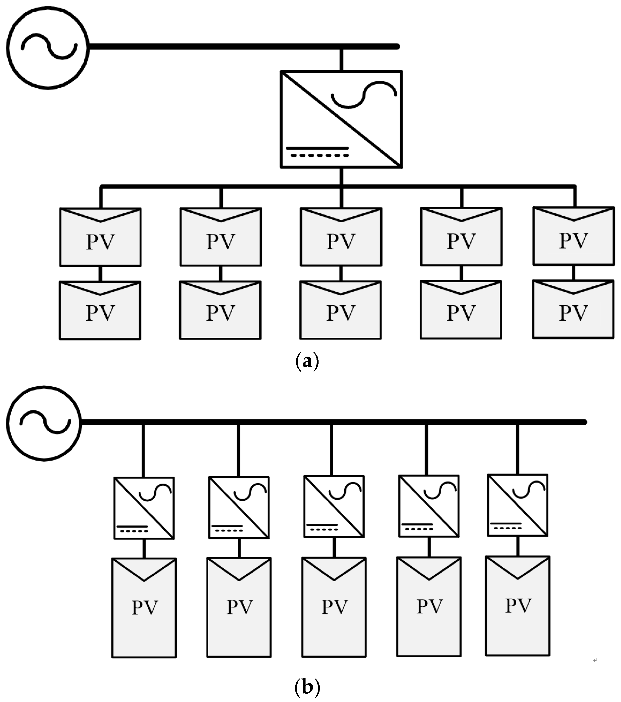
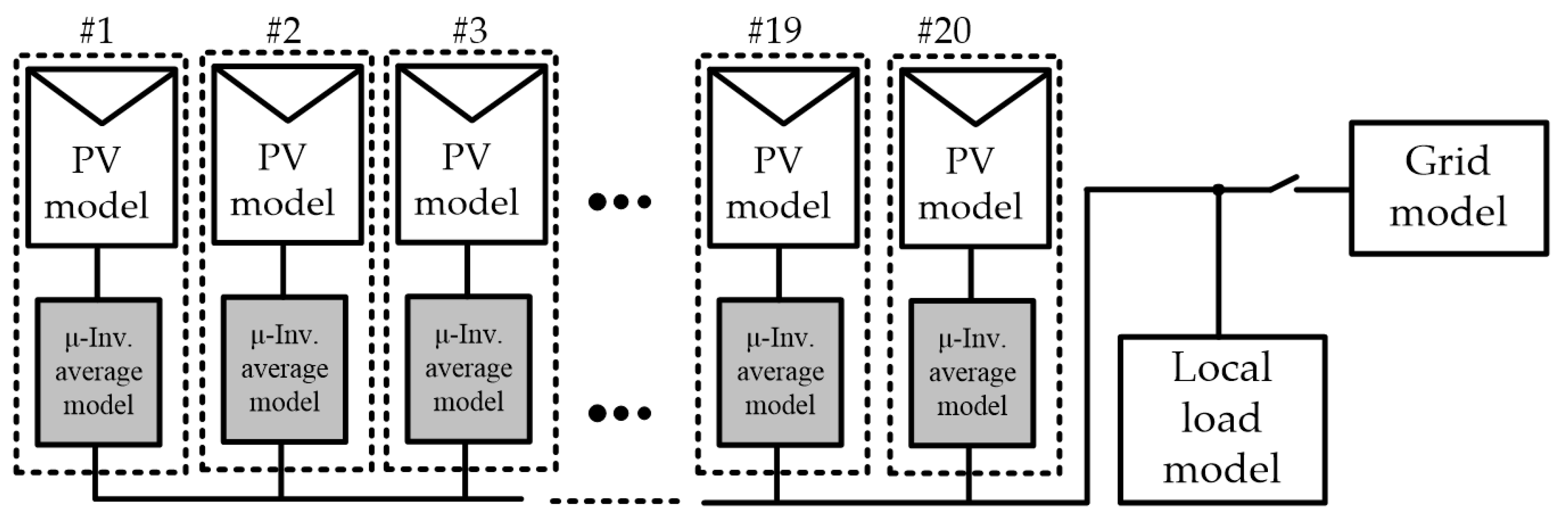
5. Aggregated Microinverter in PV Applications

In order to validate the fast simulation time of the proposed modeling approach in a multiple microinverter configuration, a simulation is carried out in MATLAB/Simulink with 20 parallel microinverters at 200 W per PV panel for a total power output of 4 kW. Figure 12 and Figure 13 show a high-level block diagram of the simulated system and the PV module model emulating PV-TD195HA6 from Mitsubishi electric corporation (Tokyo, Japan) [41], respectively. The grid voltage is at 110 Vrms, 60 Hz, and the local loads are zero (R_L → ∞). This means that all generated power from the PV modules is sent to the grid.

Partial shading is applied to some panels in order to demonstrate the simulation flexibility. Figure 14a,b show the current waveforms of the second and third microinverters among the 20 inverters where these panels have irradiance values of 900 W/m² and 800 W/m², respectively, and the irradiance of the 18 other microinverters is 1000 W/m². Another waveform shown in Figure 14a,b is that of #1 which is at 1000 W/m². Figure 14c shows the total grid current from the 20 microinverters. Resulting waveforms from using the dynamic switching model under the same conditions are shown in Figure 15. As expected, taking the average of waveforms generated using the dynamic model eliminates switching effects and the results match those in Figure 15 from the proposed average model.

Generally, the simulation runtime is highly dependent on the computer’s performance and specifications, where the simulation tool is run, and solver options. In this paper, a computer (Thinkpad T420S, Lenovo) with an Intel core i5 processor, 16 GB memory, and MATLAB 2010(a) with fixed-time step and Ode4 (Runge-Kutta) are utilized as a computational medium for simulations. Simulation runtime is compared for both average and dynamic models as shown in Figure 16.

The proposed method allows the use of a smaller step size compared to the dynamic model, thus reducing the total simulation runtime. Note that time steps ≥ 5.0 μs resulted in erratic results in the dynamic model while the average model still performed well and all signals in the simulation model were as expected.

6. Conclusions

As photovoltaic microinverter systems are typically comprised of multiple power electronic converters, a suitable modeling and simulation strategy for rapid prototyping is required. The paper has presented a time-efficient modeling and simulation strategy in multiple converter systems which can be extended to various topologies and applications, especially in the area of modeling and control of microgrids to capture finer dynamics with faster simulations. The simulation model represented by a single-matrix-form using a common or intermediate source between two average models of cascaded converters to find the overall average model was derived by employing a basic microinverter composed of a boost stage and an H-bridge. Results show that the proposed state-space average model matches experiments and dynamic simulations. The proposed model also provides significant reduction in simulation runtime and simulation set-up time with aggregated microinverters compared to the dynamic model. Larger step sizes were shown to be possible when using the average model to achieve both accurate and fast simulation convergence. Finally, the advantages of the proposed modeling and approach can be summarized as follows: (1) achieving a faster simulation time in research on aggregated multiple microinverter systems compared to dynamic switching models of converters; (2) providing better flexibility with easily interchangeable converter models; (3) understanding the relationship of state variables between multi-stage converters; and (4) simple extension to other power electronics conversion systems with multiple-stage configurations. It is expected that the proposed model will have valuable use in very large-scale PV farm simulations and can be extended for other cascaded power electronic topologies.

References

1. Scholten, D.M.; Ertugrul, N.; Soong, W.L. Micro-inverters in small scale PV systems: A review and future directions. In Proceedings of the Australasian Universities Power Engineering Conference (AUPEC), Hobart, Australia, 29 September–3 October 2013. [Google Scholar]
2. Adinolfi, G.; Graditi, G.; Siano, P.; Piccolo, A. Multi-Objective Optimal Design of Photovoltaic Synchronous Boost Converters Assessing Efficiency, Reliability and Cost Savings. IEEE Trans. Ind. Inform. 2015, 11, 1038–1048. [Google Scholar] [CrossRef]
3. Liu, C.; Sun, P.; Lai, J.S.; Ji, Y.; Wang, M.; Chen, C.L.; Cai, G. Cascade dual-boost/buck active-front-end converter for intelligent universal transformer. IEEE Trans. Ind. Electron. 2012, 59, 4671–4680. [Google Scholar]
4. Libo, W.; Zhengming, Z.; Jianzheng, L. A Single-Stage Three-Phase Grid-Connected Photovoltaic System with Modified MPPT Method and Reactive Power Compensation. IEEE Trans. Energy Convers. 2007, 22, 881–886. [Google Scholar] [CrossRef]
5. Martins, D.C. Analysis of a three-phase grid-connected PV power system using a modified dual-stage inverter. ISRN Renew. Energy 2013, 2013, 406312. [Google Scholar] [CrossRef]
6. Koran, A.; LaBella, T.; Lai, J. High efficiency photovoltaic source simulator with fast response time for solar power conditioning systems evaluation. IEEE Trans. Power Electron. 2014, 29, 1285–1297. [Google Scholar] [CrossRef]
7. Seyedmahmoudian, M.; Mekhilef, S.; Rahmani, R.; Yusof, R.; Renani, E.T. Analytical modeling of partially shaded photovoltaic systems. Energies 2013, 6, 128–144. [Google Scholar] [CrossRef]
8. Seyedmahmoudian, M.; Horan, B.; Rahmani, R.; Maung Than Oo, A.; Stojcevski, A. Efficient photovoltaic system maximum power point tracking using a new technique. Energies 2016, 9, 147. [Google Scholar] [CrossRef]
9. Aurilio, G.; Balato, M.; Graditi, G.; Landi, C.; Luiso, M.; Vitelli, M. Fast hybrid MPPT technique for photovoltaic applications: Numerical and Experimental validation. Adv. Power Electron. 2014, 2014, 125918. [Google Scholar] [CrossRef]
10. Graditi, G.; Adinolfi, G.; Femia, N.; Vitelli, M. Comparative analysis of synchronous rectification boost and diode rectification boost converter for DMPPT applications. In Proceedings of the 2011 IEEE International Symposium on Industrial Electronics (ISIE), Gdansk, Poland, 27–30 June 2011; pp. 1000–1005. [Google Scholar]
11. Graditi, G.; Adinolfi, G.; Tina, G.M. Photovoltaic optimizer boost converters: Temperature influence and electro-thermal design. Appl. Energy 2014, 115, 140–150. [Google Scholar] [CrossRef]
12. Liu, Y.; Hu, Z.; Zhang, Z.; Suo, J.; Liang, K. Research on the three-phase photovoltaic grid-connected control strategy. Energy Power Eng. 2013, 5, 31–35. [Google Scholar] [CrossRef]
13. Bojoi, R.I.; Limongi, L.R.; Roiu, D.; Tenconi, A. Enhanced power quality control strategy for single-phase inverters in distributed generation systems. IEEE Trans. Power Electron. 2011, 26, 798–806. [Google Scholar] [CrossRef]
14. Cecati, C.; Khalid, H.; Tinari, M.; Adinolfi, G.; Graditi, G. Hybrid DC Nano grid with renewable energy sources and modular DC/DC LLC converter building block. IET Power Electron. 2016, 10, 536–544. [Google Scholar] [CrossRef]
15. Hu, H.; Harb, S.; Kutkut, N.; Batarseh, I.; Shen, Z.J. A review of power decoupling techniques for microinverters with three different decoupling capacitor locations in PV systems. IEEE Trans. Power Electron. 2013, 28, 2711–2726. [Google Scholar] [CrossRef]
16. Kim, K.A.; Lertburapa, S.; Xu, C.; Krein, P.T. Efficiency and cost trade-offs for designing module integrated converter photovoltaic systems. In Proceedings of the IEEE Power and Energy Conference at Illinois, Champaign, IL, USA, 24–25 February 2012; pp. 1–7. [Google Scholar]
17. Chen, B.; Gu, B.; Zhang, L.; Zahid, Z.U.; Lai, J.-S.; Liao, Z.; Ho, R. A high-efficiency MOSFET transformer less inverter for nonisolated microinverter applications. IEEE Trans. Power Electron. 2015, 30, 3610–3622. [Google Scholar] [CrossRef]
18. Lin, F.J.; Chiang, H.C.; Chang, J.K. Modeling and controller design of PV micro inverter without using electrolytic capacitors and input current sensors. Energies 2016, 9, 993. [Google Scholar] [CrossRef]
19. Spertino, F.; Graditi, G. Power conditioning units in grid-connected photovoltaic systems: A comparison with different technologies and wide range of power ratings. Sol. Energy 2014, 108, 219–229. [Google Scholar] [CrossRef]
20. Middlebrook, R.D. Small-signal modeling of pulse-width modulated switched-mode power converters. Proc. IEEE 1988, 76, 343–354. [Google Scholar] [CrossRef]
21. Li, W.; Bélanger, J. An equivalent circuit method for modelling and simulation of modular multilevel converters in real-time HIL test bench. IEEE Trans. Power Deliv. 2016, 31, 2401–2409. [Google Scholar] [CrossRef]
22. Abramovitz, A. An approach to average modeling and simulation of switch-mode systems. IEEE Trans. Educ. 2011, 54, 509–517. [Google Scholar] [CrossRef]
23. Dijk, E.; Spruijt, J.N.; O’Sullivan, D.M.; Klaassens, J.B. PWM-switch modeling of DC-DC converters. IEEE Trans. Power Electron. 1995, 10, 659–665. [Google Scholar] [CrossRef]
24. Sun, J.; Mitchell, D.M.; Greuel, M.F.; Krein, P.T.; Bass, R.M. Averaged modeling of PWM converters operating in discontinuous conduction mode. IEEE Trans. Power Electron. 2001, 16, 482–492. [Google Scholar]
25. Suntio, T. Unified average and small-signal modeling of direct-on-time control. IEEE Trans. Ind. Electron. 2006, 53, 287–295. [Google Scholar] [CrossRef]
26. Davoudi, A.; Jatskevich, J.; Rybel, T. Numerical state-space average-value modeling of PWM DC-DC converters operating in DCM and CCM. IEEE Trans. Power Electron. 2006, 21, 1003–1012. [Google Scholar] [CrossRef]
27. Davoudi, A.; Jatskevich, J. Parasitics realization in state-space average-value modeling of PWM DC-DC converters using an equal area method. IEEE Trans. Circuits Syst. I Reg. Pap. 2007, 54, 1960–1967. [Google Scholar] [CrossRef]
28. Dupont, F.H.; Rech, C.; Gules, R.; Pinheiro, J.R. Reduced-order model and control approach for the boost converter with a voltage multiplier cell. IEEE Trans. Power Electron. 2013, 28, 3395–3404. [Google Scholar] [CrossRef]
29. Emadi, A. Modeling and analysis of multiconverter DC power electronic systems using the generalized state-space averaging method. IEEE Trans. Ind. Electron. 2004, 51, 661–668. [Google Scholar] [CrossRef]
30. Emadi, A. Modeling of power electronic loads in AC distribution systems using the generalized state-space averaging method. IEEE Trans. Ind. Electron. 2004, 51, 992–1000. [Google Scholar] [CrossRef]
31. Bina, M.Y.; Bhat, A. Averaging technique for the modeling of STATCOM and active filters. IEEE Trans. Power Electron. 2008, 23, 723–734. [Google Scholar] [CrossRef]
32. Figueres, E.; Garcera, G.; Sandia, J.; Gonzalez-Espin, F.; Rubio, J.C. Sensitivity study of the dynamics of three-phase photovoltaic inverters with an LCL grid filter. IEEE Trans. Ind. Electron. 2009, 56, 706–717. [Google Scholar] [CrossRef]
33. Krein, P.T.; Bentsman, J.; Bass, R.; Lesieutre, B.C. On the use of averaging for the analysis of power electronic systems. IEEE Trans. Power Electron. 1990, 5, 182–190. [Google Scholar] [CrossRef]
34. Meneses, D.; Blaabjerg, F.; García, O.; Cobos, J.A. Review and comparison of step-up transformerless topologies for photovoltaic AC-module application. IEEE Trans. Power Electron. 2013, 28, 2649–2663. [Google Scholar] [CrossRef]
35. Rodriguez, C.; Amaratunga, G.A.J. Analytic solution to the photo-voltaic maximum power point problem. IEEE Trans. Circuits Syst. I Reg. Pap. 2007, 54, 2054–2060. [Google Scholar] [CrossRef]
36. Park, S.M.; Bazzi, A.; Park, S.Y.; Chen, W. A time-efficient modeling and simulation strategy for aggregated multiple microinverters in large-scale PV systems. In Proceedings of the IEEE Applied Power Electronic Conference, Fort Worth, TX, USA, 16–20 March 2014. [Google Scholar]
37. Subudhi, B.; Pradhan, R. A comparative study on maximum power point tracking techniques for photovoltaic power systems. IEEE Trans. Sustain. Energy 2013, 4, 89–98. [Google Scholar] [CrossRef]
38. Mastromauro, R.A.; Liserre, M.; Dell’Aquila, A. Control issues in single-stage photovoltaic systems: MPPT, current and voltage control. IEEE Trans. Ind. Inform. 2012, 8, 241–254. [Google Scholar] [CrossRef]
39. Blaabjerg, F.; Teodorescu, R.; Liserre, M.; Timbus, A.V. Overview of control and grid synchronization for distributed power generation systems. IEEE Trans. Ind. Electron. 2006, 53, 1398–1409. [Google Scholar] [CrossRef]
40. Ma, L.; Sun, K.; Teodorescu, R.; Guerrero, J.M.; Jin, X. An integrated multifunction DC/DC converter for PV generation systems. In Proceedings of the IEEE International Symposium on Industrial Electronics, Bari, Italy, 4–7 July 2010. [Google Scholar]
41. Mitsubishi Electric Corporation. Available online: http://www.mitsubishielectric.com/bu/solar/pv_modules/pdf/L-175-0-B8492-A.pdf ( accessed on 14 February 2017).
Figure 1. PV system configurations. (a) Conventional string type; (b) multiple microinverters type.
Energies 10 00465 g001
Figure 2. General PCS structure for converting PV power.
Energies 10 00465 g002
Figure 3. Proposed modeling approach for the multiple microinverters system.
Energies 10 00465 g003
Figure 4. Multi-stage converter model with single matrix form.
Energies 10 00465 g004
Figure 5. Circuit model for deriving the average model.
Energies 10 00465 g005
Figure 6. Circuit model for the dc-dc converter.
Energies 10 00465 g006
Figure 7. Circuit model for the dc-ac converter.
Energies 10 00465 g007
Figure 8. Simulation results for a single microinverter under open-loop control with resistive load. (a) PV current; (b) dc-bus voltage; (c) ac output current.
Energies 10 00465 g008
Figure 9. Experimental results for a single microinverter under open-loop control with resistive load. (a) PV current; (b) dc-bus voltage; (c) ac output current.
Energies 10 00465 g009aEnergies 10 00465 g009b
Figure 10. Control block diagram for the microinverter. (a) dc-dc converter; (b) dc-ac converter.
Energies 10 00465 g010aEnergies 10 00465 g010b
Figure 11. Simulation results with closed-loop control. (a) PV currents; (b) dc-bus voltage; (c) ac output current.
Energies 10 00465 g011
Figure 12. Simulation structure for aggregated microinverters.
Energies 10 00465 g012
Figure 13. Electrical characteristics of the simulated PV modules under different irradiance conditions. (a) V-I curve; (b) V-P curve.
Energies 10 00465 g013
Figure 14. Simulation waveforms using the state-space average model. (a) PV currents; (b) the output currents; (c) grid voltage and current.
Energies 10 00465 g014
Figure 15. Simulation waveforms using the dynamic switching model. (a) PV currents; (b) the output currents; (c) grid voltage and current.
Energies 10 00465 g015
Figure 16. Comparison of the simulation runtime
Energies 10 00465 g016