Article

Heat Transfer and Flow of Nanofluids in a Y-Type Intersection Channel with Multiple Pulsations: A Numerical Study

1
Department of Biomedical Engineering, Carnegie Mellon University, Pittsburgh, PA 15213, USA
2
U.S. Department of Energy, National Energy Technology Laboratory (NETL), Pittsburgh, PA 15236, USA
3
School of Marine Science and Technology, Northwestern Polytechnical University, Xi’an 710072, China
*
Author to whom correspondence should be addressed.
Energies 2017, 10(4), 492; https://doi.org/10.3390/en10040492
Submission received: 11 February 2017 / Revised: 24 March 2017 / Accepted: 25 March 2017 / Published: 6 April 2017
(This article belongs to the Section I: Energy Fundamentals and Conversion)

Abstract

:
In this paper, we study pulsed flow and heat transfer in water-Al2O3 nanofluids in a Y-type intersection channel with two inlets and one outlet. At the two inlets, two sinusoidal velocities with a phase difference of π are applied. We assume that the shear viscosity and the thermal conductivity of the nanofluids depend on the nanoparticles concentration. The motion of the nanoparticles is modeled by a convention-diffusion equation, where the effects of the Brownian motion, thermophoretic diffusion, etc., are included. The effects of pulse frequency, pulse amplitude and nanoparticles concentration on the heat transfer are explored numerically at various Reynolds numbers. The results show that the application of the pulsed flow improves the heat transfer efficiency (Nusselt number) for most of the cases studied. Amongst the four factors considered, the effect of the frequency seems to be the most important.

1. Introduction

The term “heat” was first used by Carnot, as synonymous to thermal energy [1]. The importance of heat transfer in various industries, such as automotive engineering, power station engineering, air separation engineering, electronic devices cooling, etc., is well known. In the last two centuries, many thermal scientists and engineers have devoted themselves to improving the heat transfer efficiency of many processes and devices [2,3,4,5]. One of the most interesting applications of such efforts is the addition of additives to liquids (base fluids) [6] to reduce drag or to enhance heat transfer. In recent years, nanofluids, which are suspensions composed of base fluids and different types of nanoparticles, have received much attention for their outstanding performance on enhancing heat transfer efficiency [6,7,8,9,10,11,12,13,14]. In addition, nanofluids have the advantage of high mobility, better suspension stability, smaller pressure drop and less mechanical abrasion, etc. [15].
After the pioneering works by Choi [16], Eastman et al. [17], Eastman et al. [18], Xuan and Li [3], and Choi et al. [19], nanofluids have been extensively studied experimentally, theoretically and numerically [20,21,22,23,24,25,26,27,28]. In a recent review by Lomascolo et al. [29], it has been shown that the number of annual journal publications about nanofluids has been growing exponentially. Lomascolo et al. [29] provided an overview on the experimental results of the heat transfer capabilities of nanofluids, where the effects of certain parameters (size, shape, concentration, materials, etc.) on the thermal performance were systematically reviewed and analyzed. Sheikholeslami and Ganji [30] presented a review of analytical and numerical studies on flow and heat transfer of nanofluids. Two catageries of modelling methods are discussed in their paper: the single-phase approach where nanofluids are considered as single-phase fluids, and the two-component method where the behavior of the base fluid and nanoparticles are coupled but modeled separately. For more information, see the recent review articles [31,32,33].
Many researchers have also looked at producing flow disturbance for further enhancing the heat transfer. Pulsed flows are widely used in various industrial applications, such as the cooling system of gas turbine engines and the heat exchangers in milli-scale or micro-scale electronics devices where the Reynolds number (Re) is usually low and the flow is laminar [34]. Shahin [35] performed experimental and theoretical studies on the pulsed flow of a nanofluid in a pipe and in a concentric annulus, and found that the application of pulsed flow enhances and improves the heat transfer by 25% for certain flow conditions. Using the Lattice Boltzmann Method (LBM), Jafari et al. [34] performed a computational study on the effect of pulsed flow on heat transfer in a corrugated channel. They also found that the pulsed flow affects the velocity and the temperature fields leading to an enhancement of the heat transfer. Many researches have indicated that the effect of the pulsed flow on the heat transfer is rather complex. For example, Selimefendigil and Öztop [36] studied the cooling of a heated horizontal surface by a pulsating nanofluid jet; they found that compared with the steady flow, the effect of the pulse velocity is not significant at Re of 200, 400 and nanoparticles concentration of 1% and 3%. Rahgoshay et al. [15] and Nield et al. [37] reported that in a straight channel or a tube, while using a pulsed flow can change the amplitude and the phase of the fluctuating part of the local Nusselt number, no heat transfer enhancement was mentioned. Pulsed flows have been widely used in chaotic mixing in microfluidic and nanofluidic applications [38,39]. Other examples include adding fins, baffles or corrugations on the surfaces of the heat transfer devices, the application of phase change materials, etc. [40,41,42].
In this paper, we study the effect of pulsed flow of a nanofluid on the heat transfer efficiency in a Y-type intersection channel with two inlets and one outlet. Two sinusoidal velocities are applied at the inlets, having a phase difference of π, which ensures a stable flow rate in the main flow region. In Section 2, we introduce the mathematical model, which includes the governing equations and the constitutive relations. In Section 3, we discuss the geometry and the kinematics of the problems studied in this paper. In Section 4, we first test and validate our model by considering the flow in a backward step channel; we then study numerically the flow and heat transfer in a Y-type channel.

2. Mathematical Model

In general, nanofluids can be mathematically studied using three different approaches [9,30]: (1) single phase approach where the nanofluid is treated as a conventional single-phase fluid suspension with variable properties; (2) single phase non-homogenous model where the movement of the nanoparticles is modeled by a concentration-flux transport equation and the properties of the nanofluids are functions of volume fraction, temperature, shear rate, etc.; (3) two-fluid approach, such as Mixture theory approach, where the two components are coupled through interaction forces, such as drag force, shear lift force, etc. Following the paper by Buongiorno [9], the second method will be used in this paper; this approach retains several important features of the two-phase modeling, with lower computational cost.

2.1. Governing Equations

If the effects of electro-magnetism and chemical reactions are ignored, the governing equations, for a nanofluid, are the conservation equations for mass, linear and angular momentum, nanoparticle concentration/flux and energy [9,43,44,45,46].

2.1.1. Conservation of Mass

The conservation of mass reads,
ρ n f t   +   div ( ρ n f v )   =   ( 1     ϕ ) ρ f 0 t   +   div ( ( 1     ϕ ) ρ f 0 v )   +   ϕ ρ s 0 t   +   div ( ϕ ρ f 0 v )   =   0
where ρ n f = ( 1 ϕ ) ρ f 0 + ϕ ρ s 0 = α ρ f 0 + ϕ ρ s 0 is the density of the nanofluid [9]; ϕ and α are the volume fraction (concentration) of the nanoparticles and the base fluid, respectively; ρf0 and ρs0 are the pure densities of the fluid and the nanoparticles in the reference configuration (before mixing); / t is the partial derivative with respect to time; and v is the velocity vector. For an incompressible nanofluid [9], we have:
div   v = 0

2.1.2. Conservation of Linear Momentum

The conservation of linear momentum reads,
ρ n f d v d t = div   T + ρ n f b
where b is the body force vector; T is the Cauchy stress tensor; and d / d t is the total time derivative, given by d ( . )   /   d t = ( . )   / t + [ grad ( . ) ] v . The conservation of angular momentum indicates that in the absence of couple stresses the stress tensor is symmetric, i.e., T = T T .

2.1.3. Conservation of Nanoparticles Concentration/Flux

The conservation of Nanoparticles Concentration/Flux is,
ϕ t + v ϕ x = div   j
Here the first term on the left-hand side denotes the rate of change of the concentration of the nanoparticles; the second term denotes the nanoparticle flux by convection; and the term on the right hand side denotes the nanoparticle flux by diffusion. Following [45], the diffusive particle flux j is assumed to be composed of fluxes related to the Brownian motion, thermophoretic diffusion, etc. [9].

2.1.4. Conservation of Energy

The conservation of energy reads,
e t + div ( e v ) = T : L div   q + ρ r C p s j · θ
where e is the internal energy, T is the stress tensor, L is gradient of the velocity, q is the heat flux vector, r is the specific radiant energy, and C p s j · θ is the heat flux due to the diffusion of the nanoparticles [9,46]. The first term on the right hand side of the above equation is the viscous dissipation term. In this paper, we ignore the viscous dissipation and the radiation. We also do not consider the entropy inequality (Clausius-Duhem inequality), for details see the book by Liu [47].

2.2. Constitutive Equations

Nanofluids, in general, can be considered to behave as complex fluids, in the sense that they are composed of particles suspended in a fluid. In many situations it is shown that complex fluids, can be treated as a single continuum suspension with non-linear material properties (see the book by Govier and Aziz [48]). In this case, global or macroscopic information about the variables such as the velocity or the temperature fields can be obtained. In other applications, however, there is a need to know the details of the field variables such as velocity, concentration, temperature, etc.; in such cases a multi-component approach (Rajagopal and Tao [49], Massoudi [50,51]) should be taken. In this paper, we assume that the nanofluid can be considered as a single component complex fluid, where the material properties can be functions of concentration of the particles, the temperature, etc.

2.2.1. The Stress Tensor

We assume that the nanofluid can be modeled as an incompressible viscous fluid [9,46], where:
T = p I + μ n f D
where μ n f is the viscosity of the nanofluid, I is the identity tensor, p is the pressure, and D is the symmetric part of the velocity gradient. Based on the available experimental data, many nanofluids exhibit characteristics of non-linear fluids such as colloidal suspensions, polymers, etc. (see Phuoc et al. [52]). A material can be considered non-linear (from the rheological point of view) if any of the following behaviors is observed (Massoudi and Phuoc [53]): (1) the ability to shear-thin or shear-thicken; (2) the ability to creep; (3) the ability to relax stresses; (4) the presence of normal stress differences in simple shear flows; (5) the presence of yield stress. Therefore, in the single component (suspension) approach, very often it is assumed that the shear viscosity can be a function of time, shear rate, concentration, temperature, pressure, etc. Thus, in general:
μ n f = μ n f ( t , γ ˙ , θ , ϕ , p )
where t is the time, γ ˙ is some measure of the shear rate, θ is the temperature, ϕ is the concentration, and p is the pressure. In this paper, we will not consider the effects or the impact of the temperature, shear-rate, pressure and time, on the viscosity. We assume that the fluid is water-Al2O3 nanoparticles with diameter of 60 nm ; we only consider the effects of the volume fraction (concentration) on the viscosity and assume that the effective shear viscosity is modeled based on Wang’s experiments [54],
μ n f = μ f 0 ( 1 + 7.3 ϕ + 123 ϕ 2 )
The kinematic viscosity of the nanofluid is ν n f = μ n f / ρ n f . For a brief review of the viscosity of a suspension/mixture, see [50]. Next, we discuss the modeling of the particle flux j .

2.2.2. The Particle flux

In suspensions composed of solid particles and a fluid, the particles flux can be due to the Brownian motion, turbulent diffusivity, thermophoretic diffusion, particles interactions, gravity, etc. [45,55,56]. Due to the small size of the nanoparticles, the effect of particles interactions, inertia and gravity can be ignored [9,45]; thus in this paper we assume that j is given by:
j = j B + j T
where j B and j T are the contributions due to the Brownian motion and the thermophoretic diffusion, respectively. The expressions for j B and j T are given by (see [9,46] for more details),
j B = k B θ 3 π μ n f d p ϕ
j T = D T θ θ
where D T = 0.26 k n f 2 k n f + k p μ n f ρ n f ϕ [9,46], k B is the Boltzmann constant, and d p is the diameter of the nanoparticles.

2.2.3. The Internal Energy

In general, the internal energy of a fluid is given by [9,46]:
e = ρ ε
where ε is the internal energy density. In this paper, we simply assume [9,46]:
ε = c p n f θ
where c p n f is the specific heat capacity of the nanofluid. Substituting (13) into (12) and assuming that c p n f can be weighted by ϕ , we have:
e = [ ( 1 ϕ ) ρ f 0 c p f 0 + ϕ ρ s 0 c p s 0 ] θ
where c p f 0 and c p s 0 are the specific heat capacity of the pure (base) fluid and the nanoparticles in the reference configuration, i.e., before mixing. Next we discuss the modeling of the heat flux vector.

2.2.4. The Heat Flux Vector

The classical theory of heat conduction, first proposed by Fourier [57] (see also Winterton [58]) states that the heat flux vector for an isotropic material is related to the temperature gradient, where:
q = k θ
where k is the thermal conductivity of the material. For complex materials, k can depend on the concentration, the temperature, the shear rate, etc. (see Massoudi [59,60]). We use Equation (15) and assume that the suspension has an effective thermal conductivity, k n f . The effective thermal diffusivity of the nanofluids can be defined as α n f = k n f / ρ n f .
According to the review article by Lomascolo et al. [29], the thermal conductivity of a nanofluid may increase linearly with the nanoparticle volume concentration, but in some cases the increase is non-linear. Many experimental studies [61], theoretical analysis/modelling [11,61] and molecular dynamics simulations [62,63,64,65,66] have attempted to reveal the complex mechanism of the thermal conductivity of nanofluids and the heat transfer between the fluid and the nanoparticles. There have also been many studies measuring the thermal conductivity of nanofluids; proper correlations provided by these studies are useful for engineering simulations [27,67,68].
In this paper, we use the correlation proposed by Hamilton and Crosser [69] for the effective thermal conductivity, where the effect of the sphericity (through a shape factor) is also used. According to Lee et al. [70], Hamilton and Crosser ‘s model is capable of predicting the thermal conductivity of water-Al2O3 nanofluids which is studied here. Hamilton and Crosser’s correlation is:
k n f = ( ω + ( n 1 ) ( n 1 ) ( 1 ω ) ϕ ω + ( n 1 ) + ( 1 ω ) ϕ ) k f 0
where ω = k s 0 / k f 0 is the ratio of conductivity of the particle to that of the fluid, n is defined as n =   3 / ψ , where ψ is the particle sphericity which is the ratio of the surface area of a sphere (with the same volume as the given particle) to the surface area of the particle. For example, n = 3 for spheres, and n = 6 for cylinders. For a review of the effective thermal conductivity of suspensions, see [19,71].
Using Equations (6) and (8), (9)–(11) and (12)–(16) in Equations (3)–(5), we obtain a set of partial differential equations (PDEs) which need to be solved numerically. To obtain numerical solutions to these equations, we build our PDEs solver using the libraries provided by OpenFOAM [72]. The PDEs are given below:
div   v = 0
( ( 1 ϕ ) ρ f 0 + ϕ ρ s 0 ) ( v t + ( grad   v ) v ) = grad   p + div ( μ f ( 1 + 7.3 ϕ + 123 ϕ 2 ) D )
ϕ t + v ϕ x = div ( k B θ 3 π μ n f d p ϕ + 0.26 k n f 2 k n f + k p μ n f ρ n f ϕ θ θ )
( ( 1 ϕ ) ρ f 0 C p f 0 + ϕ ρ s 0 C p s 0 ) ( θ t + ( grad   θ ) v ) = div   ( ( ω + ( n 1 ) ( n 1 ) ( 1 ω ) ϕ ω + ( n 1 ) + ( 1 ω ) ϕ ) k f θ ) + ρ s 0 C p s 0 ( k B θ 3 π μ n f d p ϕ + 0.26 k n f 2 k n f + k p μ n f ρ n f ϕ θ θ ) · θ
The boundary conditions are provided in Table 1. For the velocity at the walls, a no-slip boundary condition is used; for the nanoparticles concentration, a no-flux boundary condition ensures that no particle can penetrate the wall. For more details about the boundary conditions, see [73]. We should mention that in this paper, we do not consider the effect of turbulence and the flow is assumed to be laminar throughout.
Based on the expanded governing Equations (17)–(20), we define the following non-dimensional parameters:
X = x H r ; Y = y H r ;   V = v v 0 ;   τ = t v 0 H r ;   θ ¯ = θ θ 0 θ 1 θ 0 ; R e = v 0 H r ν n f
where H r is a reference length, v 0 is a reference velocity, θ 1 is the temperature of the hot wall, and θ 0 is the inlet fluid temperature. We further define the Nusselt number, which is a measure of the ratio of the convective heat transfer to the conductive heat transfer across (normal to) the boundary. The local Nusselt number is defined as:
N u = θ ¯ n | w
The spatially averaged Nusselt number is defined as:
N u ¯ s = 1 L 0 L N u d s
The time and the spatially averaged Nusselt number is defined as:
N u ¯ s t = 1 t 1 t 0 t 0 t 1 N u ¯ s d t

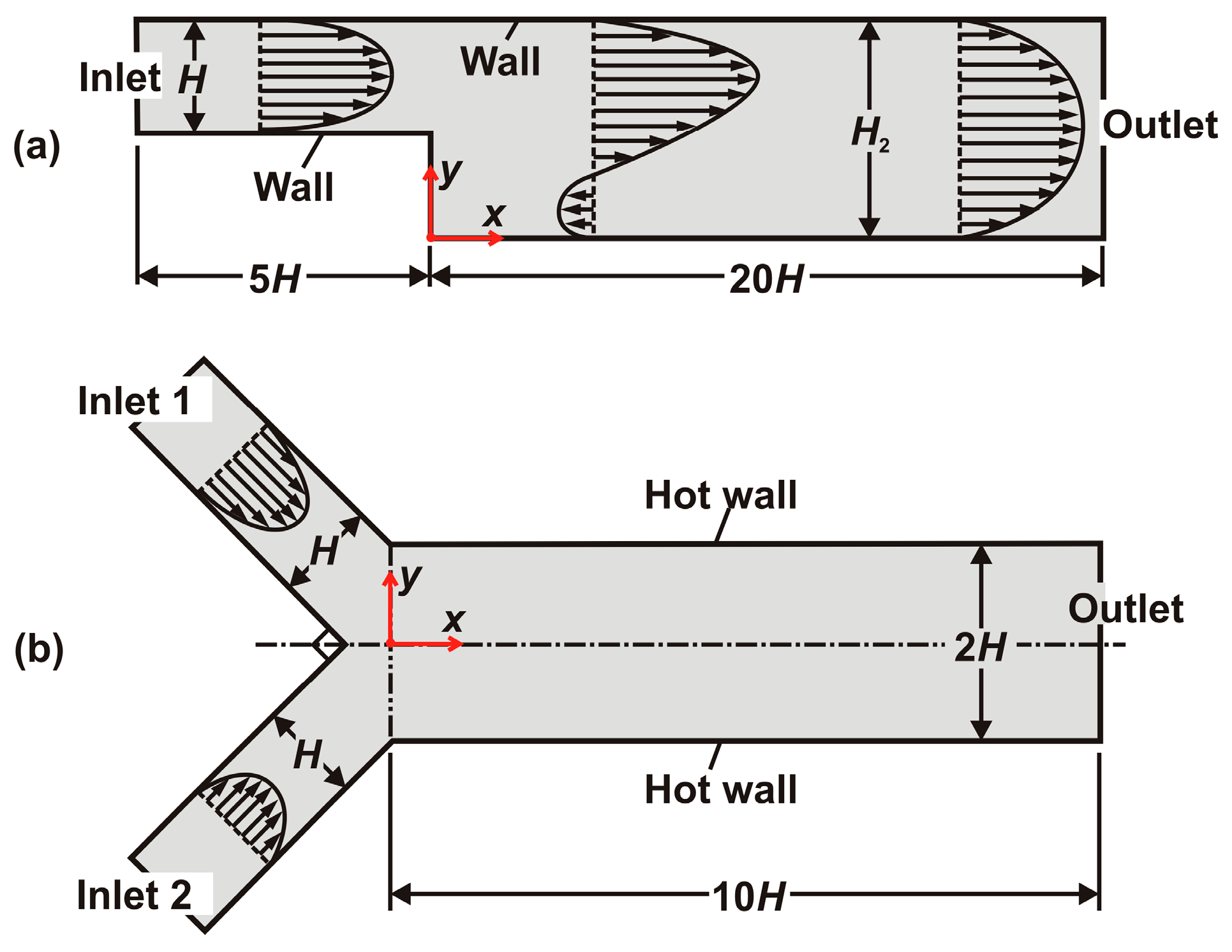
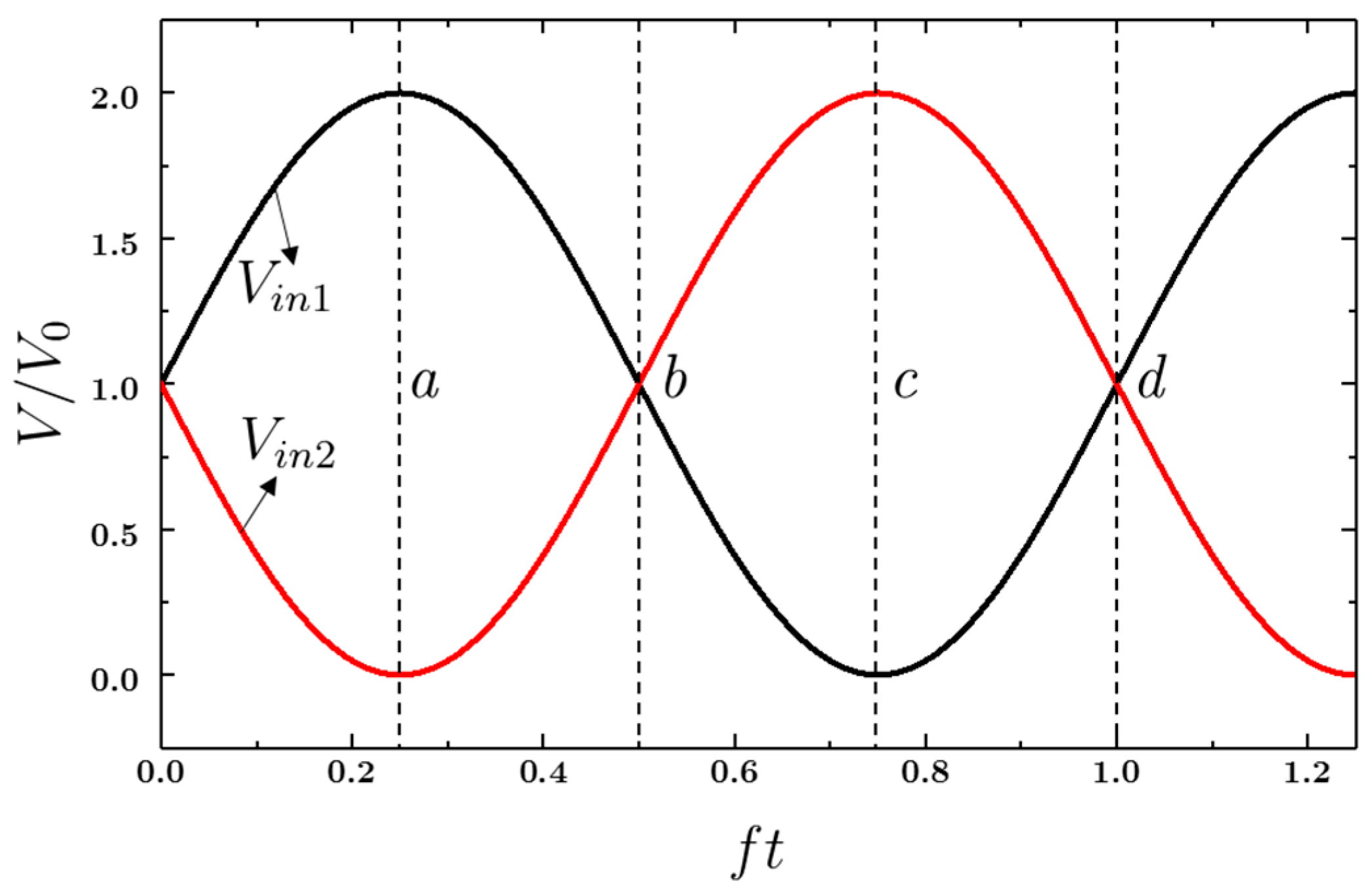
3. The Geometry and the Kinematics of the Physical Problems

The geometries of the two problems considered in this paper are shown in Figure 1. To test and validate the present model and the computational fluid dynamics (CFD) solver, we first consider the isothermal flow in a backward step channel, as shown in Figure 1a. Dimensions of the channel are based on reference [74] where the relevant experimental data are provided. The flow is assumed to be two-dimensional since the length of the channel along the z-direction is very long. More information is given in [74].
The second problem that we consider is the flow of water-Al2O3 nanofluid in a Y-type channel (Figure 1b), where the axes of the two inlets are perpendicular to each other. To reduce the computational cost, the flow is assumed to be two-dimensional. To facilitate the pulsed flow, two sinusoidal pulsed inlet velocities with a phase difference of π are applied to inlet 1 and inlet 2, expressed as:
V i n 1 = V 0 ( 1 + M p sin   ( 2 π f t ) ) V i n 2 = V 0 ( 1 + M p sin   ( 2 π f t + π ) )
where V i n 1 and V i n 2 are the applied velocities at inlet 1 and inlet 2, respectively; V 0 is the mean inlet velocity; M p is the pulse amplitude ( 0 M p 1 ); f is the pulse frequency; and t refers to time. See Figure 2 for an example of the evolution of the inlet velocity, when M p = 1 . From the above equations and Figure 2, it can be seen that in the flow region after the confluence of the two inlets, the mean velocity is always V 0 . We assume that the inlet temperatures and the initial temperature are 300 K, while the temperatures of the upper and the lower hot walls are 310 K. Other walls are adiabatic; and the concentration at the inlet is ϕ ¯ . The thermo-physical properties of the water-Al2O3 nanofluid are summarized in Table 2, where the reference temperature for k f 0 is 300 K.
For both geometries, a mesh dependency study is performed, but we only show the detail for the Y-type intersection channel. To consider the mesh dependency, we use ϕ ¯ = 0.0001 , M p = 0 , R e   = 100. Table 3 shows the time and the spatially averaged Nusselt number, N u ¯ s t , with different mesh sizes. The mesh node numbers of 21,928 and 30,062 show little difference for N u ¯ s t (less than 0.08%); therefore, in the following simulations we use the mesh with node numbers of 21,928.

4. Results and Discussion

In this section, we present our numerical results for the flow of water-Al2O3 nanofluid. We first test and validate our model and the CFD solver by solving the benchmark problem shown in Figure 1a. Then, we study the heat transfer characteristics of pulsed flow in a Y-type channel shown in Figure 1b, where the effects of the pulse frequency, Reynolds number, the pulse amplitude and the nanoparticles concentration are studied.

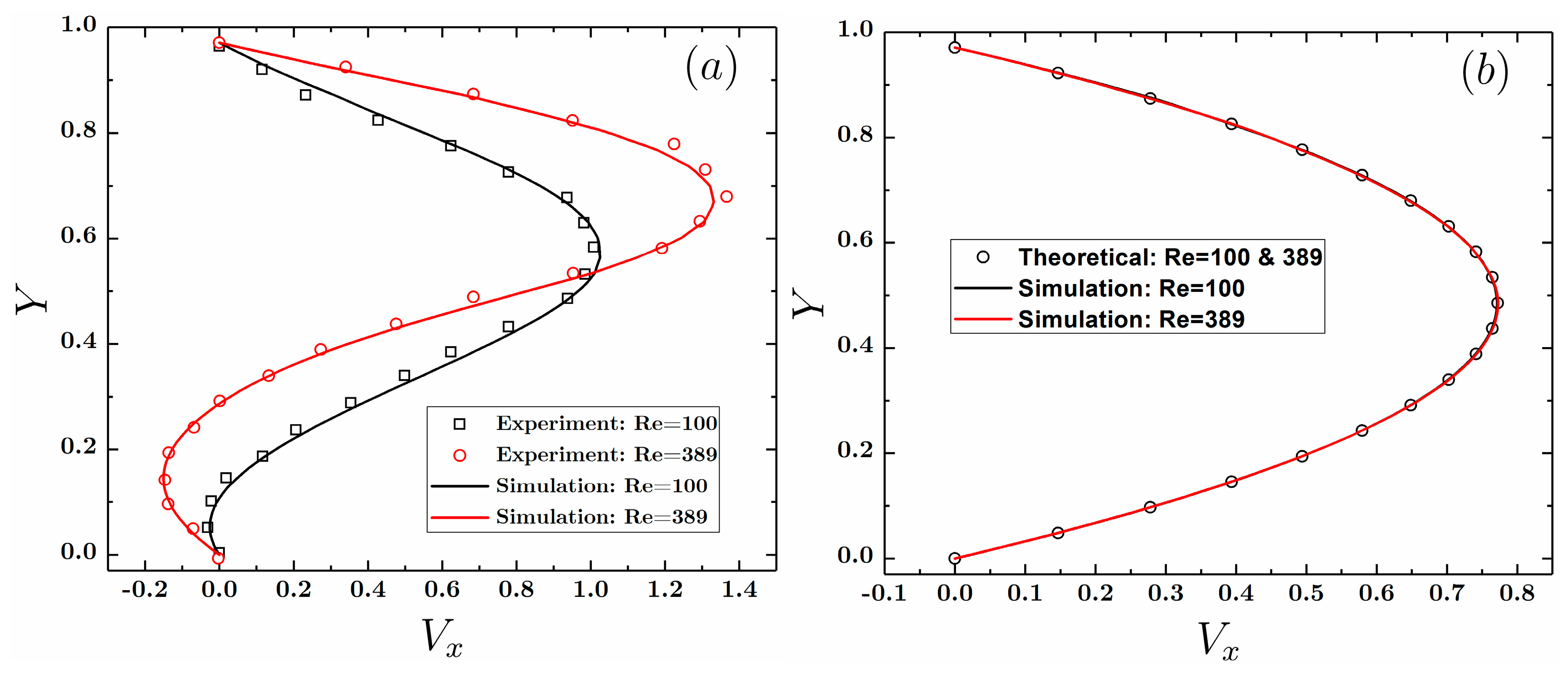
4.1. Steady Flow in a Backward-Step Channel

For this problem, the characteristic length, H r , is chosen as the hydraulic diameter of the entrance channel (before the step), which is 2H; and the reference velocity, v 0 , is the mean velocity in the entrance channel. Figure 3 shows the X-velocity profiles normalized by v 0 along the Y-direction at the dimensionless distance X = 1.28 and at the position where the flow is fully developed, with two different Reynolds numbers (100 and 389). We can see that the predicted velocity profiles agree well with the experimental measurements of Armaly et al. [74] and the theoretical predictions (parabolic profile).

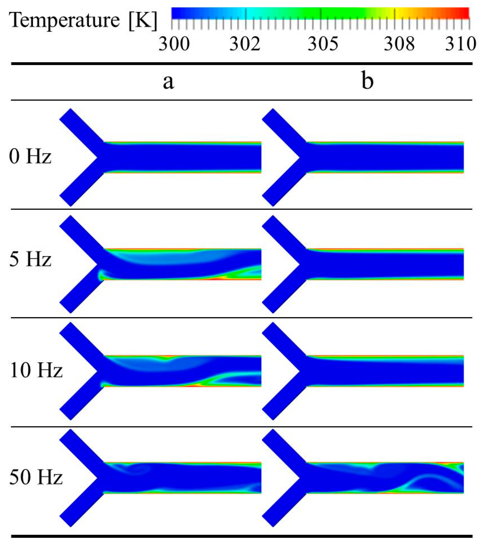
4.2. Heat Transfer Characteristics in a Y-Type Channel with Pulsed Flow

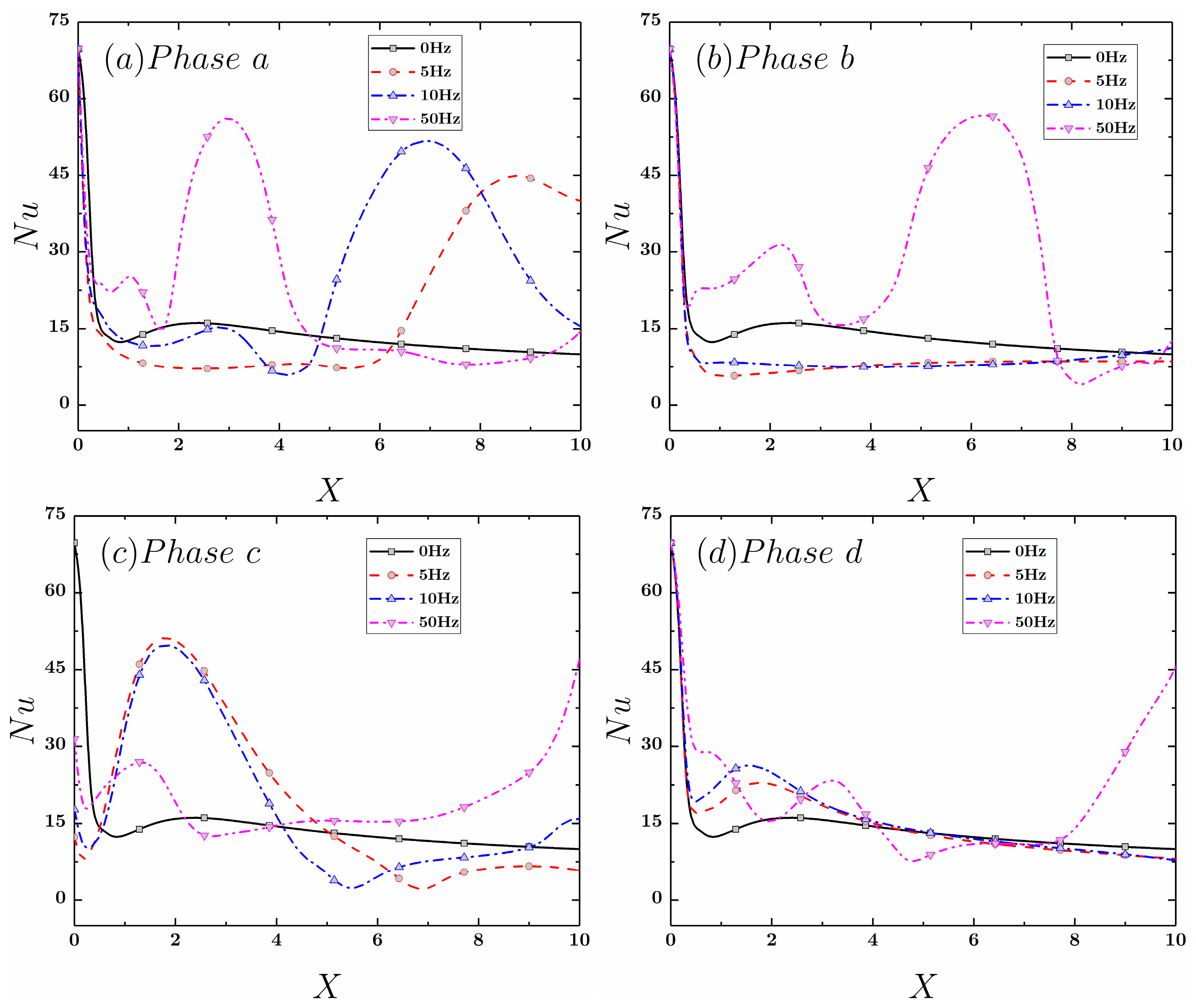
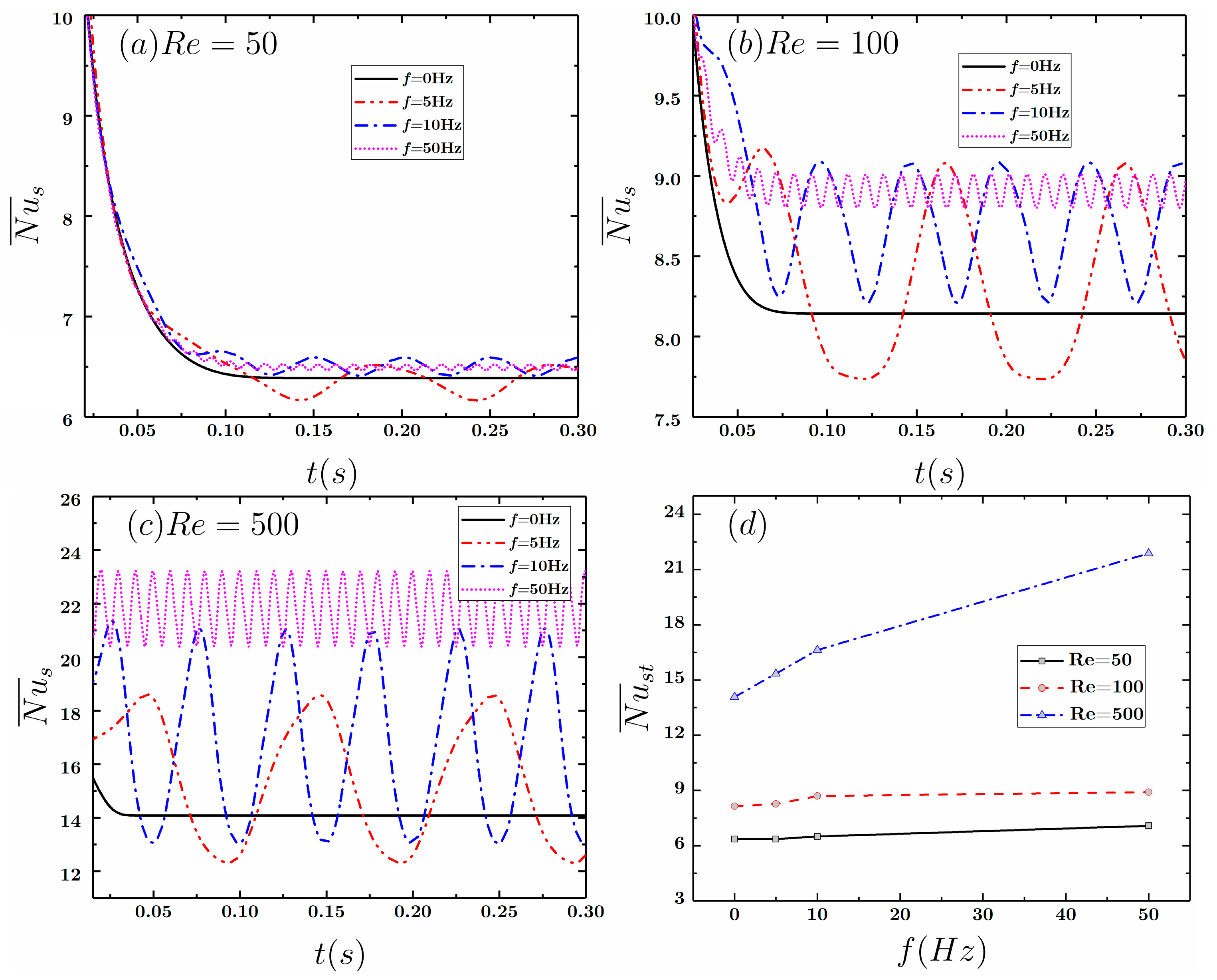
4.2.1. The Effect of Frequency

Four different values of the pulse frequency (f), are considered: 0 Hz, 5 Hz, 10 Hz and 50 Hz. The simulations are performed for ϕ ¯ = 0.05 and M p = 1 when Re = 50, 100 and 500. In Figure 2, points “a” and “b” represent the accelerating phase for inlet 2 while they represent the decelerating phase for inlet 1. Figure 4 shows the temperature fields for different pulse frequencies, when R e = 500. In this figure, “a” and “b” represent the different phase points of the pulse velocities. The temperature fields at phase points “c” and “d” are not shown because their patterns are similar Figure 4. Figure 4 indicates that for steady flows, the thermal boundary layer gradually grows along the direction of the X-axis, which implies a decrease in the temperature gradient and thus a decrease in the local Nusselt number. For the pulsed flow, when the flow is at phase point “a”, obvious temperature disturbances can be observed for all the cases. The appearance of the temperature disturbance represents the effect of the pulsed flow on the heat transfer. At several positions, the thickness of the thermal boundary layer is visibly reduced, where the temperature gradient at the walls and the local Nusselt number can be high. When the flow is at phase point “b”, for lower values the pulse frequency ( f = 5 Hz and f = 10 Hz), the temperature fields look similar to the steady flow. This implies that the effect of the pulsed flow on heat transfer is moderate. However, for the high frequency case ( f = 50 Hz), the effect is significant.
Figure 5 shows the local Nusselt number distribution on the upper (hot) wall along the X-direction at different phase points (Figure 1b) for the definition of the upper hot wall). At phase points “a” and “c”, the heat transfer enhancement expressed by the Nusselt number is obvious. At certain positions, the local Nusselt number increases significantly compared with the steady flow. For phase points “b” and “d”, only a frequency of 50 Hz shows obvious heat transfer enhancement. It should be emphasized that when the velocity is at phase point “b” and f = 0 Hz, 5 Hz and 10 Hz, the local Nusselt number is always lower than that of the steady flow. This can be attributed to the transient behavior of the inlet velocity profiles. As Figure 2 shows, V i n 1 and V i n 2 are at the decelerating phase and the accelerating phase respectively at point “b”. Before phase point “b”, V i n 1 is higher than V i n 2 ; therefore, in the region close to the upper (hot) wall, flow separation may occur and vortices develop as indicated by the temperature contours in Figure 4. At phase point “b”, although the magnitudes of the two inlet velocities become the same, the warmer fluid accumulated near the upper (hot) wall cannot be transported immediately downstream, which may be responsible for the lower convective heat transfer.
Figure 6a–c shows the time evolution of the spatially averaged Nusselt number, N u ¯ s , at different Reynolds numbers and pulse frequencies. When the simulation starts, the spatially averaged Nusselt number is relatively high; this could be attributed to the large temperature difference between the initial temperature and the temperature at the hot walls. As time passes, a thermal boundary layer is gradually formed; and as a result, the N u ¯ s decreases. Because of the pulsed flow, N u ¯ s starts oscillating periodically. The frequency of the temporal variation of N u ¯ s is the same as the frequency of the inlet pulse velocity. Figure 6 indicate that when R e = 100 and 500, some heat transfer enhancement is observed. However, when R e = 50, the effect of the pulsed flow is moderate, especially for the low frequency case ( f = 5 Hz) where N u ¯ s decreases compared to the steady flow. The heat transfer efficiency (Nusselt number) becomes more sensitive with the application of pulsed flow when the Reynolds number is high. For the same geometry, the pulse flow disturbance can be transferred to the downstream faster.
Figure 6d shows the variation of the spatial and the time averaged Nusselt number, N u ¯ s t , for different Reynolds numbers and pulse frequencies. Overall, the application of the pulsed flow enhances the heat transfer efficiency (the Nusselt number). We also see that as the R e increases, the Nusselt number increases as well. Furthermore, as f increases, the N u ¯ s t also increases for most situations.

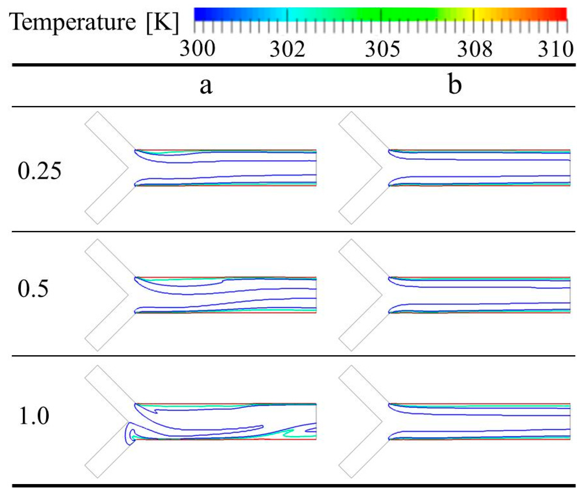
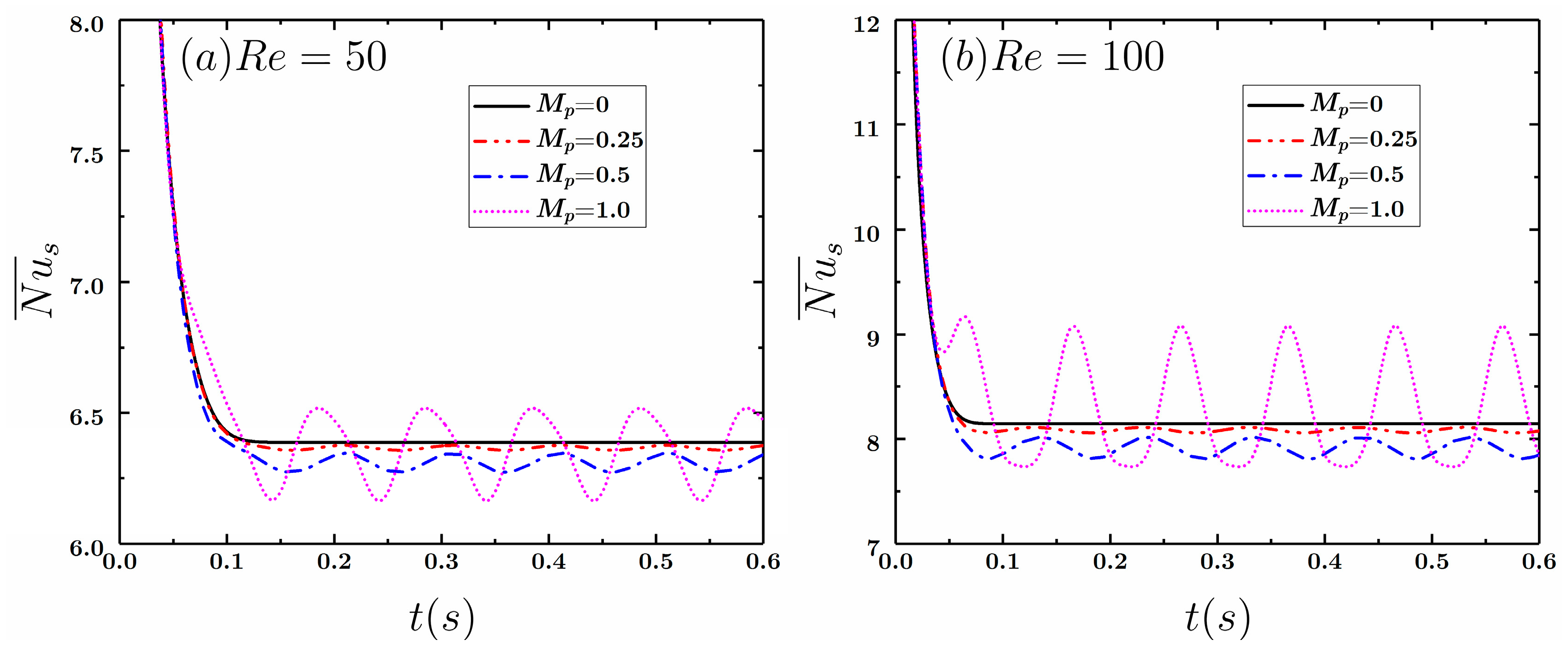
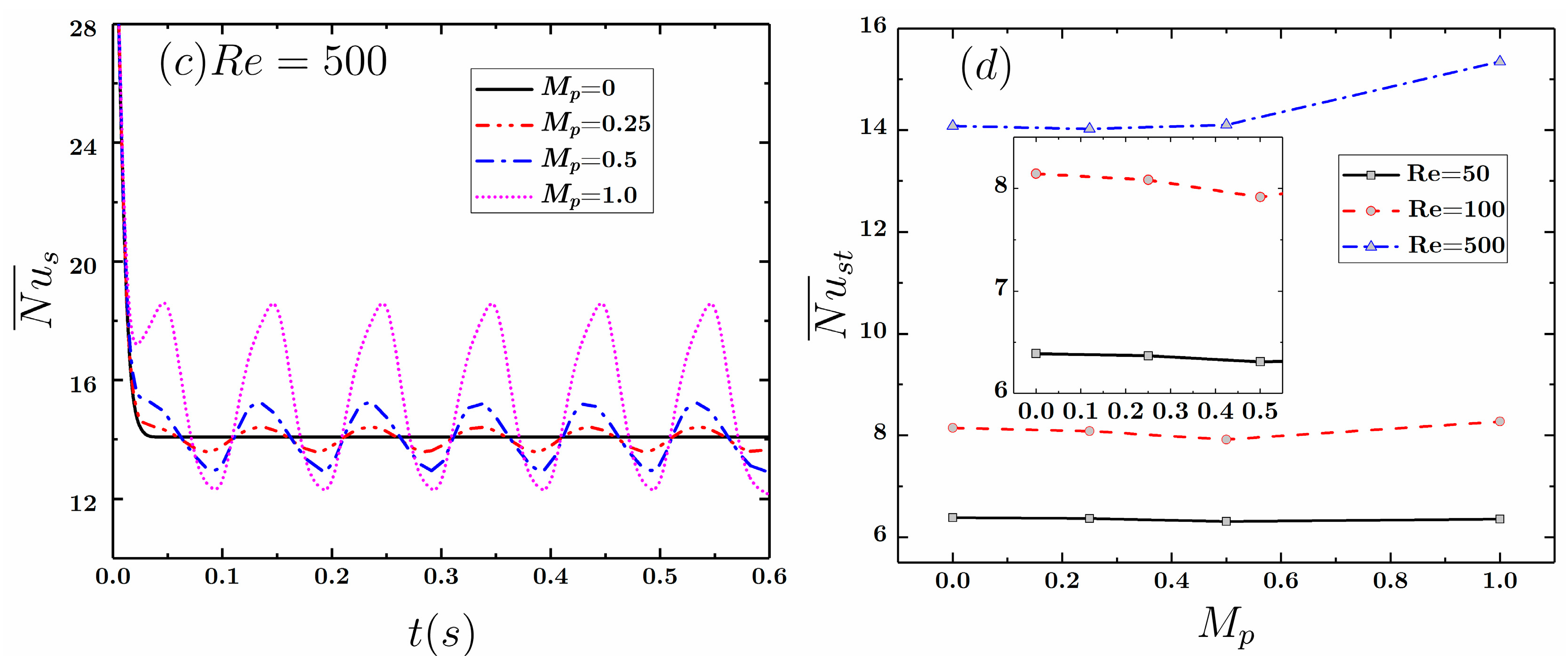
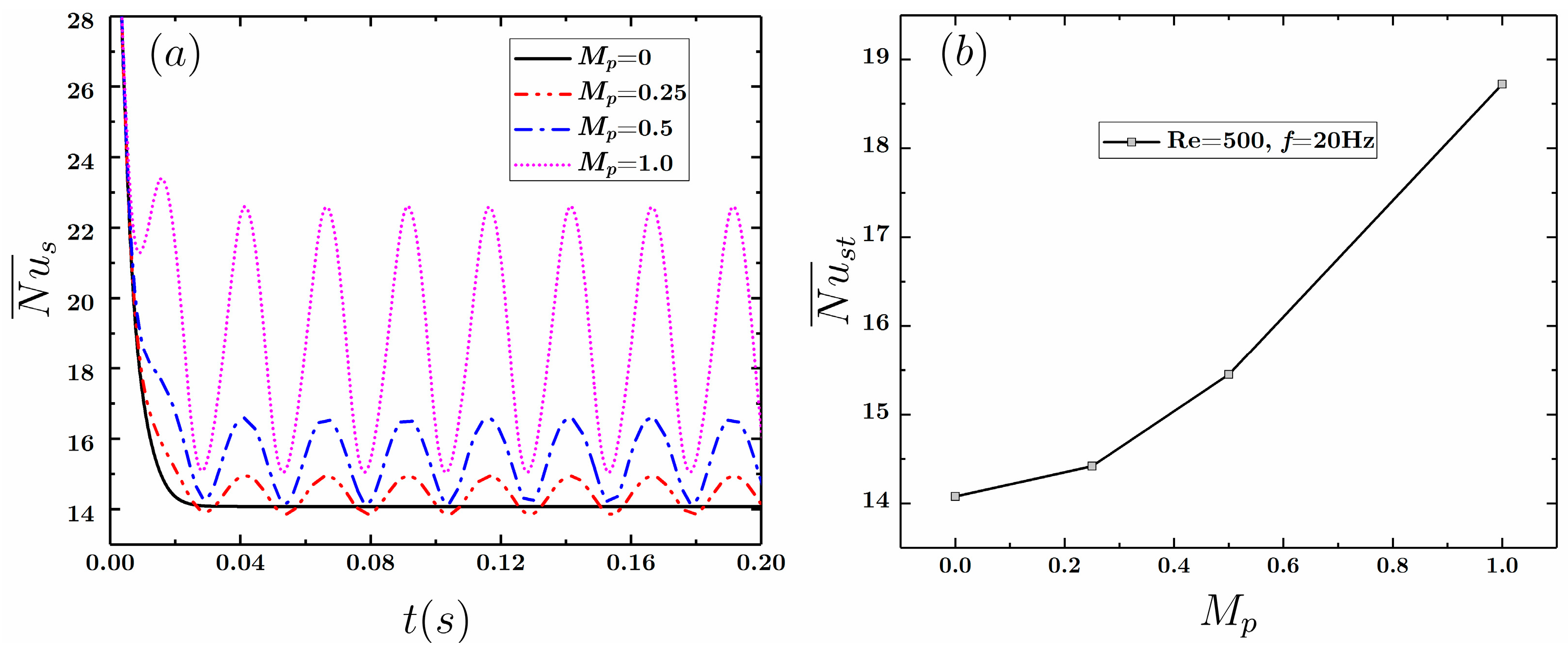
4.2.2. The Effect of the Pulse Amplitude

We consider f = 5 Hz, ϕ ¯ = 0.05 and four different values of M p : 0, 0.25, 0.5 and 1.0. The simulations are performed for three different Reynolds numbers: 50, 100 and 500. Figure 7 shows the isotherms for different values of M p , when R e = 500. At phase point “a”, as the pulse amplitude increases, the fluctuation in the isotherms increases; when the velocity is at phase point “b”, the isotherms are almost parallel to the X-direction and no disturbance can be observed.
Figure 8a–c display the effect of M p on the spatially averaged Nusselt number, N u ¯ s . when R e = 50. The application of the pulsed flow lowers the heat transfer efficiency. When R e = 100, the values of N u ¯ s with M p of 0.25 and 0.5 are still lower than the case of steady flow. When R e = 100 or 500 and M p = 1 , the N u ¯ s is larger than the N u ¯ s of steady flow. Figure 8d shows the time and the spatially averaged Nusselt number, N u ¯ s t , for different Reynolds numbers and M p . From Figure 8, we can see that only when the R e and M p are relatively large, heat transfer enhancement can be achieved for a pulsed flow. In Figure 9, we can see the effect of M p on N u ¯ s and N u ¯ s t , when R e = 500 and f = 20 Hz. As the pulse frequency is increased from 5 Hz to 20 Hz, both N u ¯ s and N u ¯ s t increase as M p increases. At higher Reynolds numbers and pulse frequency, the flow disturbance is more intensive, leading to stronger convection.

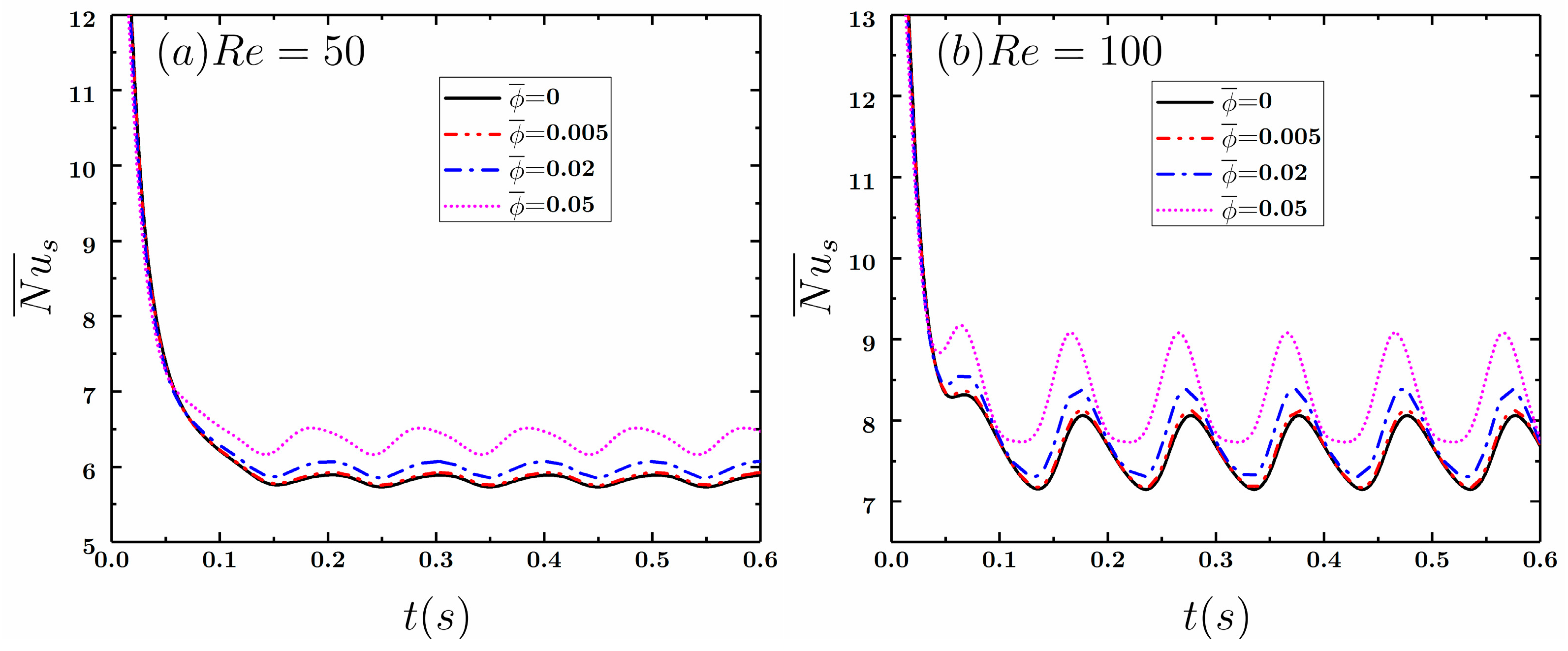
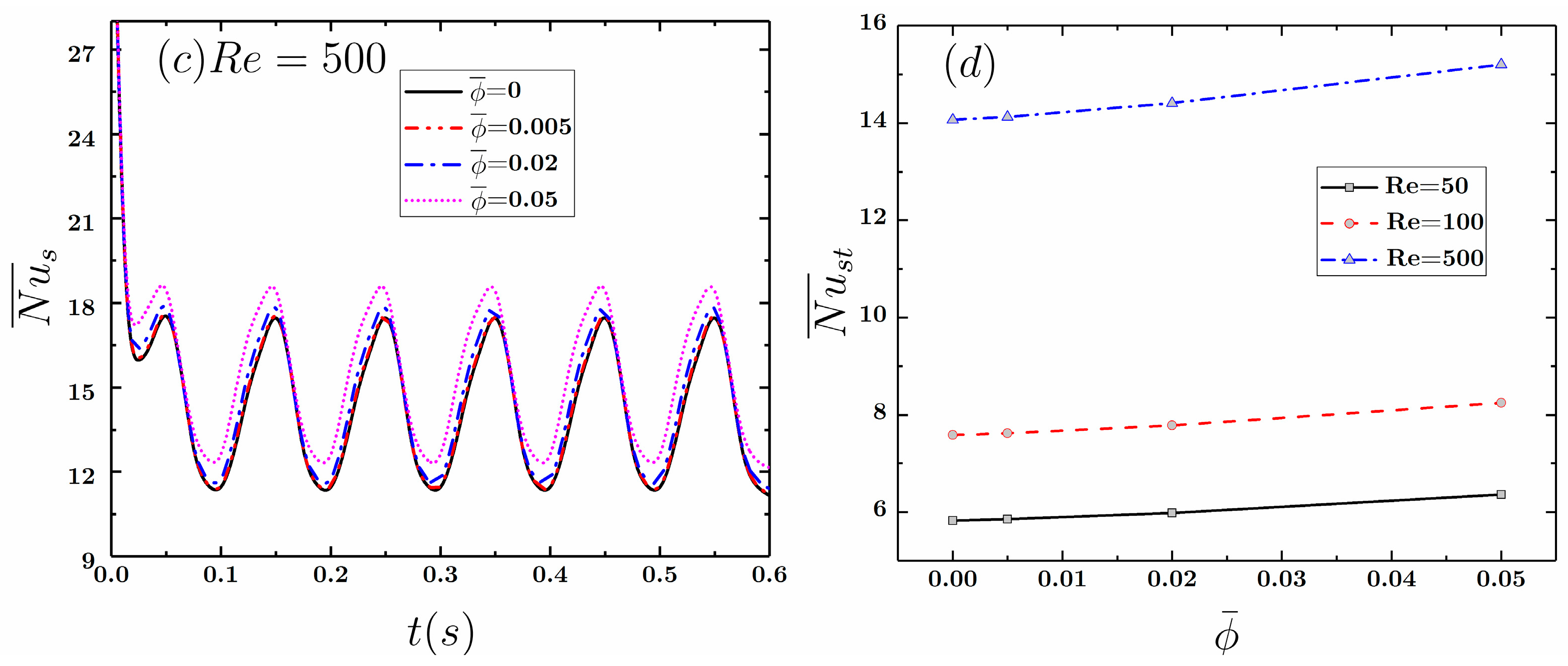
4.2.3. The Effect of Nanoparticle Concentration

Figure 10 shows the effect of the nanoparticles concentration, ϕ ¯ , when f = 5 Hz and M p = 1.0 . These figures indicate that heat transfer is enhanced, that is, as ϕ ¯ increases, there is an increase in the values of N u ¯ s and N u ¯ s t . Furthermore, in Figure 10a–c we also notice a phase shift in the oscillation of N u ¯ s , also observed by other researchers [15,36]. This could be attributed to the change in the kinematic viscosity (momentum diffusivity) of the nanofluids.

5. Conclusions

In this paper, we study the effect of pulsed flow on the heat transfer characteristics of a nanofluid in a Y-type intersection channel. The Y-type intersection channel has two inlets with two sinusoidal velocities having a phase difference of π . Our numerical studies indicate that overall, the application of the pulsed flow increases the Nusselt number, especially for large Reynolds number and high pulse frequency. Among the cases studied, the maximum enhancement of the (time and spatially averaged) Nusselt number, N u ¯ s t , is 55.4% compared with the case of steady flow. However, the results also reveal that at low Reynolds number and low pulse frequency, the pulsed flow does not improve the heat transfer efficiency. In addition, it is found that the variation of the nanoparticles concentration shifts the phase of the oscillation of the spatial averaged Nusselt number ( N u ¯ s ), believed to be related to the change of the momentum diffusivity (kinematic viscosity).

Acknowledgments

Thanks for the funding support from the Fundamental Research Funds for the Central Universities (Grant No. 3102016QD058) in China.

Author Contributions

Hongbin Yan and Wei-Tao Wu did all the numerical simulations. Wei-Tao Wu, Hongbin Yan and Mehrdad Massoudi derived all the equations. Mehrdad Massoudi supervised this work. All of the authors have provided substantial contributions to the manuscript preparation.

Conflicts of Interest

The authors declare no conflict of interest.

Nomenclature

b body force vector (N/kg)
c p f 0 specific heat of pure fluid (J/(kgK))
c p n f specific heat of nanofluid (J/(kgK))
c p s 0 specific heat of pure nanoparticles (J/(kgK))
d p diameter of nanoparticles (m)
D symmetric part of velocity gradient (s−1)
D T diffusivity of thermophoresis (m2/s)
e internal energy (J/m3)
f pulse frequency (Hz)
H height of the inlet channel (m)
H r reference length scale (m)
j particles flux (kg/(m2s))
j B particles flux (thermophoresis) (kg/(m2s))
j T particles flux (Brownian motion) (kg/(m2s))
k B Boltzmann constant (J/K)
k f 0 thermal conductivity of pure fluid (W/(mK))
k n f thermal conductivity of nanofluid (W/(mK))
k p thrmal conductivity of particles (W/(mK))
L length of the hot wall (m)
L Velocity gradient vector (s−1)
M p pulse magnitude
n dimensionless shape factor
N u local Nusselt number
N u ¯ s Spatial averaged Nusselt number
N u ¯ s t time and spatial averaged Nusselt number
p pressure (Pa)
t time
r specific radiant energy (W/kg)
q heat flux vector (W/m2)
R e Reynolds number
T stress tensor (Pa)
v 0 reference velocity (m/s)
v velocity vector (m/s)
V dimensionless velocity vector
V 0 mean inlet velocity (m/s)
V i n 1 velocity at inlet 1 (m/s)
V i n 2 velocity at inlet 2 (m/s)
x , y , z Cartesian coordinates (m)
x position vector (m)
X , Y dimensionless Cartesian coordinates
Greek symbols
α volume fraction of the base fluid
α n f thermal diffusivity of nanofluid (m2/s)
ε internal energy density (W/kg)
θ temperature (K)
θ 0 inlet fluid temperature (K)
θ 1 temperature of the hot wall (K)
μ f 0 dynamic viscosity of base fluid (Pa∙s)
μ n f dynamic viscosity of nanofluid (Pa∙s)
ν n f kinematic viscosity of nanofluid (m2/s)
ρ f 0 density of base fluid (kg/m3)
ρ n f density of nanofluid (kg/m3)
ρ s 0 density of pure nanoparticles (kg/m3)
τ dimensionless time
ϕ volume fraction of nanoparticles
ω thermal conductivity ratio

References

  1. Lienhard, J.H. A Heat Transfer Textbook; Courier Corporation: New York, NY, USA, 2013. [Google Scholar]
  2. Chen, Q.; Wang, M.; Pan, N.; Guo, Z.-Y. Optimization principles for convective heat transfer. Energy 2009, 34, 1199–1206. [Google Scholar] [CrossRef]
  3. Xuan, Y.; Li, Q. Heat transfer enhancement of nanofluids. Int. J. Heat Fluid Flow 2000, 21, 58–64. [Google Scholar] [CrossRef]
  4. Webb, R.L.; Kim, N.Y. Enhanced Heat Transfer; Taylor and Francis: New York, NY, USA, 2005. [Google Scholar]
  5. Incropera, F.P.; De Witt, D.P. Fundamentals of Heat and Mass Transfer; John Wiley & Sons, Inc.: New York, NY, USA, 1985. [Google Scholar]
  6. Li, Q.; Xuan, Y.; Wang, J. Investigation on convective heat transfer and flow features of nanofluids. J. Heat Transf. 2003, 125, 151–155. [Google Scholar]
  7. Safaei, M.R.; Ahmadi, G.; Goodarzi, M.S.; Safdari Shadloo, M.; Goshayeshi, H.R.; Dahari, M. Heat transfer and pressure drop in fully developed turbulent flows of graphene nanoplatelets–silver/water nanofluids. Fluids 2016, 1, 20. [Google Scholar] [CrossRef]
  8. Safaei, M.R.; Ahmadi, G.; Goodarzi, M.S.; Kamyar, A.; Kazi, S.N. Boundary layer flow and heat transfer of FMWCNT/water nanofluids over a flat plate. Fluids 2016, 1, 31. [Google Scholar] [CrossRef]
  9. Buongiorno, J. Convective Transport in Nanofluids. J. Heat Transf. 2006, 128, 240. [Google Scholar] [CrossRef]
  10. Ho, C.J.; Chung, Y.N.; Lai, C.-M. Thermal performance of Al2O3/water nanofluid in a natural circulation loop with a mini-channel heat sink and heat source. Energy Convers. Manag. 2014, 87, 848–858. [Google Scholar] [CrossRef]
  11. Kang, Z.; Wang, L. Effect of thermal-electric cross coupling on heat transport in nanofluids. Energies 2017, 10, 123. [Google Scholar] [CrossRef]
  12. Asirvatham, L.G.; Vishal, N.; Gangatharan, S.K.; Lal, D.M. Experimental study on forced convective heat transfer with low volume fraction of CuO/water nanofluid. Energies 2009, 2, 97–119. [Google Scholar] [CrossRef]
  13. Patil, M.S.; Kim, S.C.; Seo, J.-H.; Lee, M.-Y. Review of the thermo-physical properties and performance characteristics of a refrigeration system using refrigerant-based nanofluids. Energies 2016, 9, 22. [Google Scholar] [CrossRef]
  14. Patil, M.S.; Seo, J.-H.; Kang, S.-J.; Lee, M.-Y. Review on synthesis, thermo-physical property, and heat transfer mechanism of nanofluids. Energies 2016, 9, 840. [Google Scholar] [CrossRef]
  15. Rahgoshay, M.; Ranjbar, A.A.; Ramiar, A. Laminar pulsating flow of nanofluids in a circular tube with isothermal wall. Int. Commun. Heat Mass Transf. 2012, 39, 463–469. [Google Scholar] [CrossRef]
  16. Choi, S.U.S.; Eastman, J.A. Enhancing thermal conductivity of fluids with nanoparticles. Proceedings of 1995 International Mechanical Engineering Congress and Exhibition, San Francisco, CA, USA, 12–17 November 1995. [Google Scholar]
  17. Eastman, J.A.; Choi, S.U.S.; Li, S.; Thompson, L.J.; Lee, S. Enhanced thermal conductivity through the development of nanofluids. In MRS Proceedings; Cambridge University Press: Cambridge, UK, 1996; Volume 457, p. 3. [Google Scholar]
  18. Eastman, J.A.; Choi, S.U.S.; Li, S.; Yu, W.; Thompson, L.J. Anomalously increased effective thermal conductivities of ethylene glycol-based nanofluids containing copper nanoparticles. Appl. Phys. Lett. 2001, 78, 718–720. [Google Scholar] [CrossRef]
  19. Choi, S.U.S.; Zhang, Z.G.; Yu, W.; Lockwood, F.E.; Grulke, E.A. Anomalous thermal conductivity enhancement in nanotube suspensions. Appl. Phys. Lett. 2001, 79, 2252–2254. [Google Scholar] [CrossRef]
  20. Xie, Y.; Zheng, L.; Zhang, D.; Xie, G. Entropy generation and heat transfer performances of Al2O3-water nanofluid transitional flow in rectangular channels with dimples and protrusions. Entropy 2016, 18, 148. [Google Scholar] [CrossRef]
  21. Li, P.; Xie, Y.; Zhang, D.; Xie, G. Heat transfer enhancement and entropy generation of nanofluids laminar convection in microchannels with flow control devices. Entropy 2016, 18, 134. [Google Scholar] [CrossRef]
  22. Elbashbeshy, E.M.A.; Emam, T.G.; Abdel-Wahed, M.S. Flow and heat transfer over a moving surface with nonlinear velocity and variable thickness in a nanofluid in the presence of thermal radiation. Can. J. Phys. 2013, 92, 124–130. [Google Scholar] [CrossRef]
  23. Kumar Ch, K.; Bandari, S. Melting heat transfer in boundary layer stagnation-point flow of a nanofluid towards a stretching–shrinking sheet. Can. J. Phys. 2014, 92, 1703–1708. [Google Scholar] [CrossRef]
  24. Mustafa, I.; Javed, T.; Majeed, A. Magnetohydrodynamic (MHD) mixed convection stagnation point flow of a nanofluid over a vertical plate with viscous dissipation. Can. J. Phys. 2015, 93, 1365–1374. [Google Scholar] [CrossRef]
  25. Colangelo, G.; Favale, E.; de Risi, A.; Laforgia, D. Results of experimental investigations on the heat conductivity of nanofluids based on diathermic oil for high temperature applications. Appl. Energy 2012, 97, 828–833. [Google Scholar] [CrossRef]
  26. Mintsa, H.A.; Roy, G.; Nguyen, C.T.; Doucet, D. New temperature dependent thermal conductivity data for water-based nanofluids. Int. J. Therm. Sci. 2009, 48, 363–371. [Google Scholar] [CrossRef]
  27. Gu, B.; Hou, B.; Lu, Z.; Wang, Z.; Chen, S. Thermal conductivity of nanofluids containing high aspect ratio fillers. Int. J. Heat Mass Transf. 2013, 64, 108–114. [Google Scholar] [CrossRef]
  28. Nnanna, A.G. Experimental model of temperature-driven nanofluid. J. Heat Transf. 2007, 129, 697–704. [Google Scholar] [CrossRef]
  29. Lomascolo, M.; Colangelo, G.; Milanese, M.; de Risi, A. Review of heat transfer in nanofluids: Conductive, convective and radiative experimental results. Renew. Sustain. Energy Rev. 2015, 43, 1182–1198. [Google Scholar] [CrossRef]
  30. Sheikholeslami, M.; Ganji, D.D. Nanofluid convective heat transfer using semi analytical and numerical approaches: A review. J. Taiwan Inst. Chem. Eng. 2016, 65, 43–77. [Google Scholar] [CrossRef]
  31. Fang, X.; Chen, Y.; Zhang, H.; Chen, W.; Dong, A.; Wang, R. Heat transfer and critical heat flux of nanofluid boiling: A comprehensive review. Renew. Sustain. Energy Rev. 2016, 62, 924–940. [Google Scholar] [CrossRef]
  32. Bigdeli, M.B.; Fasano, M.; Cardellini, A.; Chiavazzo, E.; Asinari, P. A review on the heat and mass transfer phenomena in nanofluid coolants with special focus on automotive applications. Renew. Sustain. Energy Rev. 2016, 60, 1615–1633. [Google Scholar] [CrossRef]
  33. Kasaeian, A.; Azarian, R.D.; Mahian, O.; Kolsi, L.; Chamkha, A.J.; Wongwises, S.; Pop, I. Nanofluid flow and heat transfer in porous media: A review of the latest developments. Int. J. Heat Mass Transf. 2017, 107, 778–791. [Google Scholar] [CrossRef]
  34. Jafari, M.; Farhadi, M.; Sedighi, K. Pulsating flow effects on convection heat transfer in a corrugated channel: A LBM approach. Int. Commun. Heat Mass Transf. 2013, 45, 146–154. [Google Scholar] [CrossRef]
  35. Shahin, G.A. The Effect of Pulsating Flow on Forced Convective Heat Transfer. Master’s Thesis, University of Western Ontario, London, ON, Canada, 1998. [Google Scholar]
  36. Selimefendigil, F.; Öztop, H.F. Pulsating nanofluids jet impingement cooling of a heated horizontal surface. Int. J. Heat Mass Transf. 2014, 69, 54–65. [Google Scholar] [CrossRef]
  37. Nield, D.A.; Kuznetsov, A.V. Forced convection with laminar pulsating flow in a channel or tube. Int. J. Therm. Sci. 2007, 46, 551–560. [Google Scholar] [CrossRef]
  38. Glasgow, I.; Aubry, N. Enhancement of microfluidic mixing using time pulsing. Lab Chip 2003, 3, 114–120. [Google Scholar] [CrossRef] [PubMed]
  39. Goullet, A.; Glasgow, I.; Aubry, N. Effects of microchannel geometry on pulsed flow mixing. Mech. Res. Commun. 2006, 33, 739–746. [Google Scholar] [CrossRef]
  40. Elbahjaoui, R.; El Qarnia, H. Transient behavior analysis of the melting of nanoparticle-enhanced phase change material inside a rectangular latent heat storage unit. Appl. Therm. Eng. 2017, 112, 720–738. [Google Scholar] [CrossRef]
  41. Mashaei, P.R.; Taheri-Ghazvini, M.; Moghadam, R.S.; Madani, S. Smart role of Al2O3-water suspension on laminar heat transfer in entrance region of a channel with transverse in-line baffles. Appl. Therm. Eng. 2017, 112, 450–463. [Google Scholar] [CrossRef]
  42. Ho, C.J.; Chen, Y.Z.; Tu, F.-J.; Lai, C.-M. Thermal performance of water-based suspensions of phase change nanocapsules in a natural circulation loop with a mini-channel heat sink and heat source. Appl. Therm. Eng. 2014, 64, 376–384. [Google Scholar] [CrossRef]
  43. Zhou, Z.; Wu, W.-T.; Massoudi, M. Fully developed flow of a drilling fluid between two rotating cylinders. Appl. Math. Comput. 2016, 281, 266–277. [Google Scholar] [CrossRef]
  44. Slattery, J.C. Advanced Transport Phenomena; Cambridge University Press: Cambridge, UK, 1999. [Google Scholar]
  45. Phillips, R.J.; Armstrong, R.C.; Brown, R.A.; Graham, A.L.; Abbott, J.R. A constitutive equation for concentrated suspensions that accounts for shear-induced particle migration. Phys. Fluids A Fluid Dyn. 1992, 4, 30–40. [Google Scholar] [CrossRef]
  46. Tzou, D.Y. Thermal instability of nanofluids in natural convection. Int. J. Heat Mass Transf. 2008, 51, 2967–2979. [Google Scholar] [CrossRef]
  47. Liu, I.-S. Continuum Mechanics; Springer Science & Business Media: Berlin, Germany, 2002. [Google Scholar]
  48. Govier, G.W.; Aziz, K. The Flow of Complex Mixtures in Pipes; Krieger Pub Co: Malabar, FL, USA, 1977. [Google Scholar]
  49. Rajagopal, K.R.; Tao, L. Mechanics of Mixtures; Series on Advances in Mathematics for Applied Sciences; World Scientific Publishing: Singapore, 1995; Volume 35. [Google Scholar]
  50. Massoudi, M. A note on the meaning of mixture viscosity using the classical continuum theories of mixtures. Int. J. Eng. Sci. 2008, 46, 677–689. [Google Scholar] [CrossRef]
  51. Massoudi, M. A Mixture Theory formulation for hydraulic or pneumatic transport of solid particles. Int. J. Eng. Sci. 2010, 48, 1440–1461. [Google Scholar] [CrossRef]
  52. Phuoc, T.X.; Massoudi, M.; Chen, R.-H. Viscosity and thermal conductivity of nanofluids containing multi-walled carbon nanotubes stabilized by chitosan. Int. J. Therm. Sci. 2011, 50, 12–18. [Google Scholar] [CrossRef]
  53. Massoudi, M.; Phuoc, T.X. Remarks on constitutive modeling of nanofluids. Adv. Mech. Eng. 2012, 2012, 927580. [Google Scholar] [CrossRef]
  54. Wang, X.; Xu, X.; Choi, S.U.S. Thermal conductivity of nanoparticle-fluid mixture. J. Thermophys. Heat Transf. 1999, 13, 474–480. [Google Scholar] [CrossRef]
  55. Subia, S.R.; Ingber, M.S.; Mondy, L.A.; Altobelli, S.A.; Graham, A.L. Modelling of concentrated suspensions using a continuum constitutive equation. J. Fluid Mech. 1998, 373, 193–219. [Google Scholar] [CrossRef]
  56. Wu, W.-T.; Massoudi, M. Heat transfer and dissipation effects in the flow of a drilling fluid. Fluids 2016, 1, 4. [Google Scholar] [CrossRef]
  57. Fourier, J. The Analytical Theory of Heat; Dover Publications: New York, NY, USA, 1955. [Google Scholar]
  58. Winterton, R.H.S. Early study of heat transfer: Newton and Fourier. Heat Transf. Eng. 2001, 22, 3–11. [Google Scholar] [CrossRef]
  59. Massoudi, M. On the heat flux vector for flowing granular materials—Part I: Effective thermal conductivity and background. Math. Methods Appl. Sci. 2006, 29, 1585–1598. [Google Scholar] [CrossRef]
  60. Massoudi, M. On the heat flux vector for flowing granular materials—Part II: Derivation and special cases. Math. Methods Appl. Sci. 2006, 29, 1599–1613. [Google Scholar] [CrossRef]
  61. Iacobazzi, F.; Milanese, M.; Colangelo, G.; Lomascolo, M.; de Risi, A. An explanation of the Al2O3 nanofluid thermal conductivity based on the phonon theory of liquid. Energy 2016, 116, 786–794. [Google Scholar] [CrossRef]
  62. Milanese, M.; Iacobazzi, F.; Colangelo, G.; de Risi, A. An investigation of layering phenomenon at the liquid–solid interface in Cu and CuO based nanofluids. Int. J. Heat Mass Transf. 2016, 103, 564–571. [Google Scholar] [CrossRef]
  63. Sarkar, S.; Selvam, R.P. Molecular dynamics simulation of effective thermal conductivity and study of enhanced thermal transport mechanism in nanofluids. J. Appl. Phys. 2007, 102, 74302. [Google Scholar] [CrossRef]
  64. Kim, B.H.; Beskok, A.; Cagin, T. Molecular dynamics simulations of thermal resistance at the liquid-solid interface. J. Chem. Phys. 2008, 129, 174701. [Google Scholar] [CrossRef] [PubMed]
  65. Kim, B.H.; Beskok, A.; Cagin, T. Thermal interactions in nanoscale fluid flow: Molecular dynamics simulations with solid–liquid interfaces. Microfluid. Nanofluid. 2008, 5, 551–559. [Google Scholar] [CrossRef]
  66. Vo, T.Q.; Park, B.; Park, C.; Kim, B. Nano-scale liquid film sheared between strong wetting surfaces: Effects of interface region on the flow. J. Mech. Sci. Technol. 2015, 29, 1681–1688. [Google Scholar] [CrossRef]
  67. Colangelo, G.; Favale, E.; Miglietta, P.; Milanese, M.; de Risi, A. Thermal conductivity, viscosity and stability of Al2O3-diathermic oil nanofluids for solar energy systems. Energy 2016, 95, 124–136. [Google Scholar] [CrossRef]
  68. Sundar, L.S.; Farooky, M.H.; Sarada, S.N.; Singh, M.K. Experimental thermal conductivity of ethylene glycol and water mixture based low volume concentration of Al2O3 and CuO nanofluids. Int. Commun. Heat Mass Transf. 2013, 41, 41–46. [Google Scholar] [CrossRef]
  69. Hamilton, R.L.; Crosser, O.K. Thermal conductivity of heterogeneous two-component systems. Ind. Eng. Chem. Fundam. 1962, 1, 187–191. [Google Scholar] [CrossRef]
  70. Li, S.; Eastman, J.A. Measuring thermal conductivity of fluids containing oxide nanoparticles. J. Heat Transf 1999, 121, 280–289. [Google Scholar]
  71. Wang, X.-Q.; Mujumdar, A.S. Heat transfer characteristics of nanofluids: A review. Int. J. Therm. Sci. 2007, 46, 1–19. [Google Scholar] [CrossRef]
  72. OpenFOAM Programmer’s Guide Version 2.1.0; The OpenFOAM Foundation: London, UK, 2011.
  73. Rusche, H. Computational Fluid Dynamics of Dispersed Two-Phase Flows at High Phase Fractions; Imperial College London (University of London): London, UK, 2002; Volume 1. [Google Scholar]
  74. Armaly, B.F.; Durst, F.; Pereira, J.C.F.; Schönung, B. Experimental and theoretical investigation of backward-facing step flow. J. Fluid Mech. 1983, 127, 473–496. [Google Scholar] [CrossRef]
  75. Job, V.M.; Gunakala, S.R. Mixed convection nanofluid flows through a grooved channel with internal heat generating solid cylinders in the presence of an applied magnetic field. Int. J. Heat Mass Transf. 2017, 107, 133–145. [Google Scholar] [CrossRef]
  76. Barbés, B.; Páramo, R.; Blanco, E.; Pastoriza-Gallego, M.J.; Piñeiro, M.M.; Legido, J.L.; Casanova, C. Thermal conductivity and specific heat capacity measurements of Al2O3 nanofluids. J. Therm. Anal. Calorim. 2013, 111, 1615–1625. [Google Scholar] [CrossRef]
  77. Sridhara, V.; Satapathy, L.N. Al2O3-based nanofluids: A review. Nanoscale Res. Lett. 2011, 6, 456. [Google Scholar] [CrossRef] [PubMed]
  78. Touloukian, Y.S.; Powell, R.W.; Ho, C.Y.; Nicolaou, M.C. Thermophysical Properties of Matter-The TPRC Data Series. Volume 10. Thermal Diffusivity; DTIC Document: Bedford, MA, USA, 1974. [Google Scholar]
  79. Xie, H.; Wang, J.; Xi, T.; Liu, Y.; Ai, F.; Wu, Q. Thermal conductivity enhancement of suspensions containing nanosized alumina particles. J. Appl. Phys. 2002, 91, 4568–4572. [Google Scholar] [CrossRef]
Figure 1. Two-dimensional illustration of the physical problems: (a) Isothermal flow in a backward step channel where H2 = 1.9423H [74]; (b) Pulsed flow and heat transfer in a Y-type channel where the two inlet channels are perpendicular to each other.
Energies 10 00492 g001
Figure 2. Temporal variation of the non-dimensional inlet velocities (V/V0) where “a”, “b”, “c“ and “d” represent different phase points of the pulsed velocity, respectively.
Energies 10 00492 g002
Figure 3. (a) Dimensionless velocity distribution along the Y-direction at X = 1.28 obtained from simulations and the experiments at Reynolds numbers of 100 and 389; (b) Fully developed dimensionless velocity distribution along the Y-direction obtained from simulations and the theoretical prediction at Reynolds numbers of 100 and 389. Notice that when Re = 389, the simulation is performed in a longer channel for achieving fully developed flow.
Energies 10 00492 g003
Figure 4. Temperature fields corresponding to different pulse frequencies at representative phase points “a” and “b” of the pulse inlet velocities.
Energies 10 00492 g004
Figure 5. Spatial distribution of the local Nusselt number evaluated at the upper (hot) wall along X-direction at different phase points: (a) Phase a; (b) Phase b; (c) Phase c; and (d) Phase d.
Energies 10 00492 g005
Figure 6. Time evolution of the spatially averaged Nusselt number, N u ¯ s , with different pulse frequencies when (a) Re = 50; (b) Re = 100 and (c) Re = 500; and (d) Time-spatially averaged Nusselt number, N u ¯ s t , as a function of the pulse frequency and the Reynolds number.
Energies 10 00492 g006
Figure 7. Isotherm distribution with different pulse amplitudes, M p , at phase points “a” and “b” of the pulse velocity when R e = 500.
Energies 10 00492 g007
Figure 8. Time evolution of the spatially averaged Nusselt number, N u ¯ s , with different pulse amplitudes when (a) Re = 50; (b) Re = 100 and (c) Re = 500; and (d) Time-spatially averaged Nusselt number, N u ¯ s t , as a function of the pulse amplitude and the Reynolds number.
Energies 10 00492 g008aEnergies 10 00492 g008b
Figure 9. (a) Time evolution of the spatially averaged Nusselt number, N u ¯ s , with different pulse amplitudes when the Reynolds number is 500 and the pulse frequency is 20 Hz; (b) Time-spatially averaged Nusselt number, N u ¯ s t , as a function of the pulse amplitude when the Reynolds number is 500 and the pulse frequency is 20 Hz.
Energies 10 00492 g009
Figure 10. Time evolution of the spatially averaged Nusselt number, N u ¯ s , with different nanoparticle concentrations when (a) Re = 50; (b) Re = 100; (c) Re = 500; and (d) Time-spatially averaged Nusselt number, N u ¯ s t , as a function of the nanoparticle concentration and the Reynolds number.
Energies 10 00492 g010aEnergies 10 00492 g010b
Table 1. Boundary conditions used in our numerical simulations.
Boundary TypePressureVelocityConcentrationTemperature
WallFixed flux (0)Fixed valueFixed flux (0)Fixed value or flux
InletFixed value (0)Fixed valueFixed value (0)Fixed value
OutletFixed value (0)Fixed flux (0)Fixed flux (0)Fixed flux (0)
Table 2. Physical properties of the water-Al2O3 nanofluid considered in the present study.
Physical PropertyValuePhysical PropertyValue
ρ f 0 1000 kg/m3 [36,75] c p f 0 4180 J/(kg∙K) [36,75]
ρ s 0 3600 kg/m3 [36,76] c p s 0 784 J/(kg∙K) [76]
d p 60 nm [77] k f 0 0.604 W/(m∙K) [78,79]
μ f 1.0 cP [36,75] ω 76.3 [78,79]
Table 3. Time-spatial averaged Nusselt number, N u ¯ s t , with different meshes for the Y-type channel.
Mesh SizeThe Nusselt Number, N u ¯ s t
10,52012.81
17,22112.65
21,92812.62
30,06212.61

