
Dynamic Simulation of an Organic Rankine Cycle—Detailed Model of a Kettle Boiler


Institute for Energy Systems, Department of Mechanical Engineering, Technical University of Munich, Garching bei München, 85748, Germany
*
Author to whom correspondence should be addressed.
Energies 2017, 10(4), 548; https://doi.org/10.3390/en10040548
Submission received: 1 March 2017
/
Revised: 10 April 2017
/
Accepted: 12 April 2017
/
Published: 17 April 2017
Abstract
:Organic Rankine Cycles (ORCs) are nowadays a valuable technology to produce electricity from low and medium temperature heat sources, e.g., in geothermal, biomass and waste heat recovery applications. Dynamic simulations can help improve the flexibility and operation of such plants, and guarantee a better economic performance. In this work, a dynamic model for a multi-pass kettle evaporator of a geothermal ORC power plant has been developed and its dynamics have been validated against measured data. The model combines the finite volume approach on the tube side and a two-volume cavity on the shell side. To validate the dynamic model, a positive and a negative step function in heat source flow rate is applied. The simulation model performed well in both cases. The liquid level appeared the most challenging quantity to simulate. A better agreement in temperature was achieved by increasing the volume flow rate of the geothermal brine by 2% over the entire simulation. Measurement errors, discrepancies in working fluid and thermal brine properties and uncertainties in heat transfer correlations can account for this. In the future, the entire geothermal power plant will be simulated, and suggestions to improve its dynamics and control by means of simulations will be provided.
1. Introduction
Organic Rankine Cycles (ORCs) have been increasingly applied to produce electricity from low and medium temperature sources in the last decade. The reported global installed capacity has currently surpassed 2700 MWe, and an additional 523.6 MWe have been planned [1]. Typical application fields for ORC are geothermal, biomass, solar thermal and low grade waste heat recovery plants [2,3,4]. The size of ORC plants can vary from few kWe to some MWe [4,5]. Several studies report the advantages of organic fluids in comparison to water for low and medium temperature small-size power plants [5,6,7]. As an example, in [8,9] the organic fluid resulted to be better performing than water and air for a heat source temperature below 300 °C.
Given the modest temperature of the source, the electrical efficiency of ORCs is generally less than 20% [2,4]. The remaining energy is either dissipated through piping, compression and expansion machines, heat losses, auxiliary consumption and heat transfer to the condenser. The heat rejected to the condenser can be recovered to provide thermal energy for district heating, commercial buildings and industrial processes. In this case, the ORC is designed to work in combined heat and power (CHP) mode, providing electricity and heat with a relatively high energy utilization factor [10,11,12]. A comparison of the different configurations for ORC in CHP mode is provided in [13].
A simple ORC system consists of four main elements: a preheater/evaporator, where the working fluid is preheated and vaporized at saturated state or slightly superheated, an expansion machine, where the thermal energy of the fluid is converted into rotational energy of the expander shaft, a condenser, where the fluid is cooled down and condensed back to liquid state, and a pump, which brings the condensed liquid to the evaporation pressure to start the process cycle again. A recuperator might be applied, being advantageous mainly for dry fluids. Sub-, trans- and supercritical ORCs with pure organic fluids and their mixtures have also been investigated [14,15,16,17,18,19,20,21]. Supercritical ORCs might offer higher system efficiencies in dependency of the temperature source, at the expenses of higher investment and maintenance costs. The reduced temperature difference at the evaporator causes higher investment costs, because of the larger heat transfer surface and the higher pressure that the evaporator has to withstand [15,22]. For dry fluids, superheating has no positive effect and should be avoided, since it increases the complexity of the evaporator and the thermal stresses on the expansion machine [23].
The evaporator is the crucial component that links the ORC to the heat source/heat transfer medium, and its design is therefore of major relevance for the thermodynamic, hydraulic and economic performance of the ORC. For mobile applications, the heat exchanger has to be additionally optimized in terms of volume and weight [24,25,26].
In the following, the main configurations of evaporators for stationary ORC are considered. Fin-and-tube heat exchangers are mainly applied for waste heat recovery from gas turbine and internal combustion engines [27,28,29]. The extended surface of the shell side improves the heat transfer for the exhaust gas, whereas the working fluid shows a heat transfer coefficient of at least two orders of magnitude higher and flows inside the tubes [28]. The pressure drop of the exhaust gas on the shell side has a negative impact on the performance of the topping cycle and should be minimized [30,31,32]. Shell-and-tube heat exchangers are applied or assumed for ORC optimization in different studies [33,34,35,36]. This type of heat exchanger can be deployed up to very high pressures and temperatures, has a relatively simple geometry and its design and manufacturing procedures are very well-known and established [37]. Plate heat exchangers might be advantageous for low pressure, low temperature applications thanks to their compactness, effectiveness, easiness to be cleaned, maintained or extended [38]. As a major drawback, plate heat exchangers increase the pressure losses, especially for exhaust gas waste heat recovery, because of the narrow channels. A comparison between shell-and-tube and plate heat exchangers is carried out in [39].
In large size subcritical ORCs, kettle boilers are often used as evaporators [6]. The preheating of the organic fluid generally occurs in once-through shell-and-tube heat exchangers, whereas the evaporation takes place in the kettle boiler. The heating fluid, e.g., thermal brine for a geothermal power plant, passes through the tubes in a single- or multi-pass scheme. If no superheating is desired, the tube bundle is completely submerged in the liquid pool. The boiler disposes of a freeboard at the top of the kettle for separation of the vapor and liquid phase [37]. The vapor is then extracted from the top of the boiler, and fed to the expander. The effective separation between liquid and vapor in a kettle boiler gives more flexibility in power plant operation. In fact, in case of sudden variation of the input source, the boiler responds with a variation in pressure and/or level, avoiding that droplets get entrained to the turbine inlet [40]. In off-design conditions, some tubes may lay above the liquid level, leading to some degree of superheating and hence ensuring that no droplets are carried out to the expander inlet. In case of tube exposed to the vapor, tube material limits should not be overcome as a result of the higher wall temperature. The dynamic flexibility gives a significant advantage to kettle boilers with respect to tube once-through boilers. In the latter some degree of superheating is always necessary for safety reason, and a more demanding control is required to ensure pure vapor conditions at the expander inlet [40]. The pool boiler configuration is also recently being mentioned for mixtures of organic fluids [40]. An accurate evaporator design has also to consider the response of the heat exchanger in transient conditions. Dynamic simulations of ORC power plants are, in fact, gaining significant interest for a number of reasons:
- To increase the energy conversion efficiency, power plants must be able to respond very fast and in an optimal way to variations in heat source or ambient conditions (e.g., waste heat recovery systems);
- The presence of hot spots in heat exchangers during transients can be limited, avoiding thermal degradation of the working fluid [46];
- The increasing complexity in the dynamics of the electricity grid, associated with the increasing penetration of variable-source renewables (i.e., wind and photovoltaics), requires a higher contribution from controllable power plants (biomass, geothermal) for security margin, load reserve and grid stability;
- Renewables-based ORCs could be used as stand-alone systems in remote areas and operated under strong dynamic conditions [47];
- Start-ups, shutdowns and emergency situations (turbine trips, safety valve lifting) can also take help from dynamic simulations [50].
Dynamic models of ORC have been mainly developed in the Modelica® language (Modelica Association, Linköping, Sweden) [51]. The equation-based, object-oriented and a-causal nature of the modelling language makes it very suitable for simulation of nonlinear thermo-fluid systems, such as ORC power plants [47,52]. The different plant components are developed as “individual objects” which can be connected to each other. The objects are generally compiled in libraries. Different libraries for thermo-fluid systems are available, either open-source or commercial [53]. Several software codes based on this modelling language are available, such as Dymola, SimulationX, JModelica or OpenModelica [54]. Thermodynamic and transport properties of the fluid are generally accessed by means of external fluid property libraries, e.g., NIST Reference Fluid and Transport Properties Database (REFPROP), FluidProp, CoolProp or TILMedia [55,56,57,58]. The focus of these dynamic tools is generally on the overall plant performance and the interaction among components rather than on the detailed description of the single elements, which is generally carried out with more demanding tools, such as Computational Fluid Dynamics (CFD) or Finite Element Methods (FEM) [47].
The broad application of kettle boilers for middle and large size ORCs, together with the increasing interest in ORC dynamics and simulation, require a valid model for the dynamic simulation of this component. The complex geometrical arrangement makes also current models unsuitable for this scope. In this paper, a dynamic model of a kettle evaporator is developed and validated with measured data. The model has the advantage of high simulation speed, good accuracy and a high flexibility for different heat exchanger geometries.
The dynamic modelling of heat exchangers and in particular evaporators for ORC systems is discussed in the next section. A closer insight into the proposed model for the kettle boiler is gained in Section 2. Validation and results are reported in Section 3, followed by a discussion in Section 4. A brief summary and conclusions are found at the end of this paper.
Dynamic Modelling of Evaporators for Organic Rankine Cycles
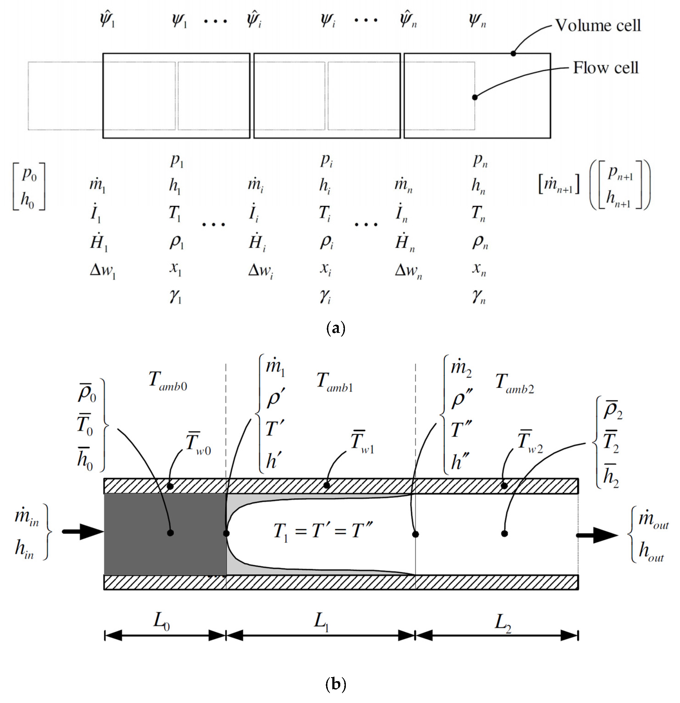
Dynamic models of heat exchangers (and not only) are based on the principle laws of mass, energy and momentum conservation, and integrated by empirical correlation to account for specific properties or characteristics of the system. The models are typically discretized over the length of the heat exchangers (1-D). The choice of the state variables for fluid property computation is discussed in [59,60]. The state variables have a strong impact on how the differential-algebraic equations (DAE) are solved. Most of the tools nowadays use pressure and specific enthalpy as state variables. The state of the solid wall of heat exchangers is defined by the wall temperature. The way the equations are numerically solved defines the type of dynamic model used for the heat exchanger. The most common types are (conceptually depicted in Figure 1):
- Finite volumes (FV);
- Moving boundary (MB).
The FV method is based on a static discretization of the heat exchanger in a given number of cells of equal volume. According to the degree of subcooling at the inlet and/or superheating at the outlet of the heat exchanger, the fluid in a cell can be in liquid, vapor or two-phase. On one hand, a higher number of cells is generally desired for higher accuracy of the solution. On the other hand, the computational time increases with the number of cells. A trade-off has to be found between the accuracy of the solution and the computational time. A major problem occurs with the FV method applied to a phase-change heat exchanger. This can be explained looking at the continuity equation:
where is the fluid density, the cell volume, the incoming and the outgoing fluid mass flow rate. Since the saturated liquid line shows a large discontinuity in density when the fluid passes from the liquid to the two-phase region, the time derivative of the density can become very high. If the inlet mass flow rate is given, a fast density change can cause peaks in resulting in flow reversal, chattering or non-solvable solutions. The simulation can become extremely slow or even fail [61].
MB refers to fast low-order dynamic models that subdivide the heat exchanger in a liquid, vapor and two-phase control volume. If one of the regions is not present, the corresponding volume is neglected. The volumes dynamically change their length according to the thermodynamic conditions in the heat exchangers. Techniques to account dynamically for the presence of each control volume are also available [62]. In the two-phase region, the average density is computed in MB methods by means of the average void fraction, according to [63]:
where is the average void fraction, and and are the densities of saturated liquid and vapor. Assumptions on the average void fraction have to be made. The validity of the assumption has an impact on the accuracy of the dynamic simulation [63].
The MB and FV models have been compared in [59,63,64]. The MB model requires less computation time than FV, even though the accuracy is typically lower. The MB model could preferably be applied for online control systems, rather than system simulation [59,60]. The computation of the amount of working fluid present in the cycle (also called charge) is critical for both models because of the absence of high-accuracy correlations for the void fraction in the evaporator and condenser. The MB model has however shown worse results between the two [64].
Another modeling approach can be used when a fluid changes phase in a large shell or pool, and the heating/cooling medium flows in a tube bundle. The evaporating/condensing fluid can be represented by means of two volumes (TV) in thermal non-equilibrium. The TV are modelled with a lumped approach, as in the MB model. Unlike the MB model, however, the mass transfer between the TV is a function of the vapor quality in each of the TV, and not a result of the mass and momentum equation at the cell boundaries. As an example, in case of the evaporator, when the vapor quality in the liquid phase is bigger than zero, the liquid is vaporizing, so mass is transferred from the liquid to the vapor region. These mass transfers are independent from the outer direction of flow, which is pressure driven. A TV model for a shell-and-tube condenser is included in the ThermoSysPro library in Modelica® and discussed in [65].
An accurate model of the evaporator is essential to reproduce the dynamic behavior of ORC. As an example, most of the control strategies are based on the degree of superheating at the evaporator outlet, or on the evaporation pressure [41]. The thermal inertia and time response of the evaporator have a crucial impact on how source fluctuations affect the dynamics and control of the power plant. While for small-scale ORC once-through heat exchangers of simple geometry are applied, kettle boilers are very often used in larger scale ORC. Because of the more complex geometry of the kettle, FV and MB cannot represent properly the dynamics of this heat exchanger. In the present work, a dynamic model of a kettle boiler is developed by means of a combination between TV (for the shell-side) and FV method (for the tube/wall side) and validated against measurements from an analogous heat exchanger located in a geothermal power plant in the Munich area. The present work is based on the commercial TIL-Library (Version 3.2.2, TLK-Thermo GmbH, Braunschweig, Germany [66]). The basic models have been taken from this library, and new components have been developed based on the existing library. The resulting combined TV/FV model can be used for design, off-design and dynamic simulations, and applied for testing and development of basic or advanced control strategies for middle and large-scale ORC power plants.
2. TV/FV Model for the Kettle Boiler
In this section, the theory and equations necessary for the modeling of the kettle boiler are described. It is very important to limit the complexity of the model, in order to allow for its integration in a closed-loop cycle simulation, without incurring in extremely large simulation time or simulation failures.
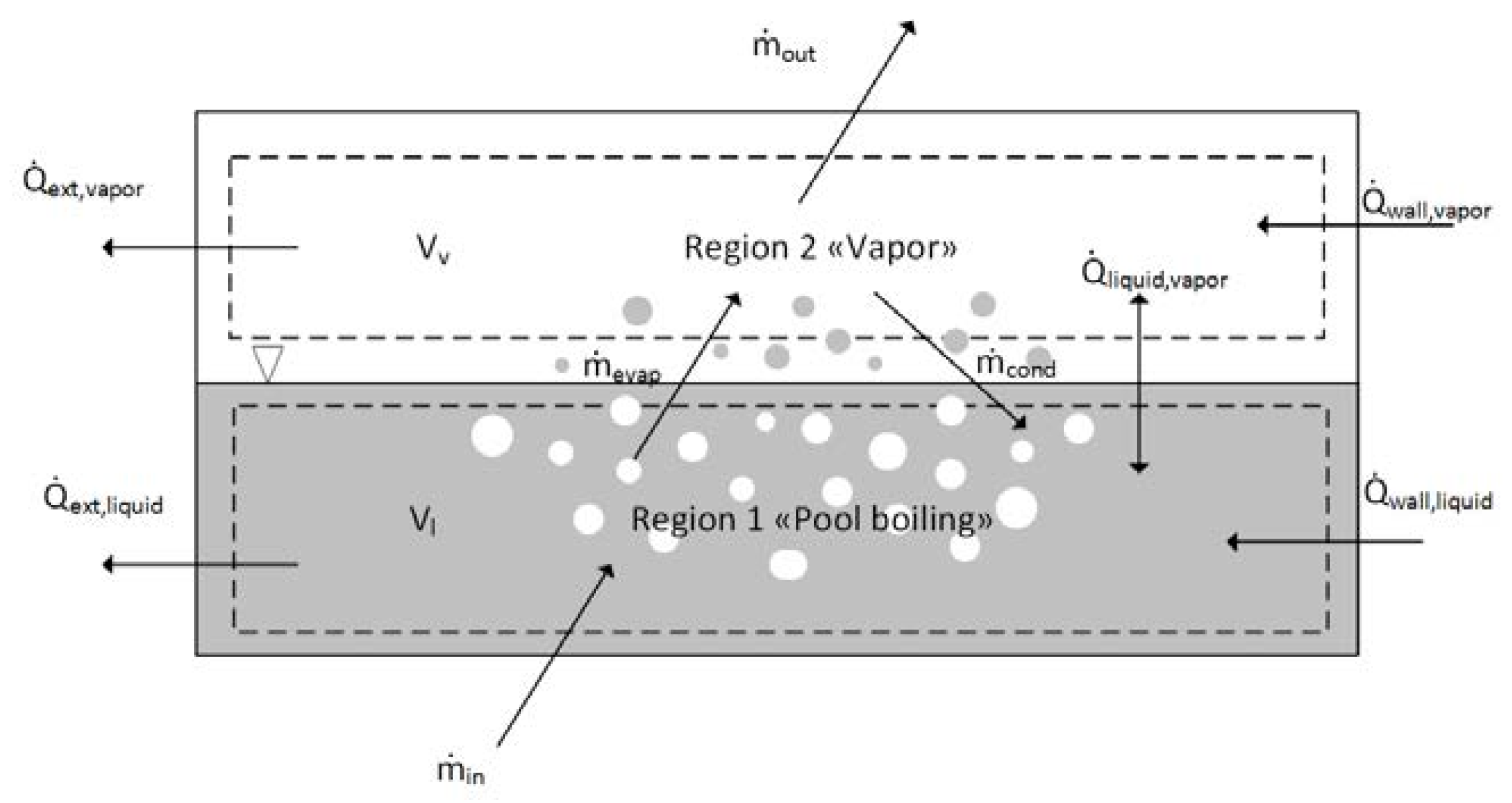
2.1. Two-Volume Cavity
The shell-side of the kettle boiler is modelled by means of a TV cavity (TVC), shown in Figure 2. The lower volume (Region 1, grey) represents the vaporizing liquid, whereas the upper volume (Region 2, white) describes the vapor region. The laws of conservation for mass, momentum and energy are developed for each (lumped) volume, which are in general in thermal non-equilibrium. The TVC can exchange mass according to the vapor quality of the volumes. If the vapor quality in the Region 1 is larger than zero, a mass flow will be transferred from Region 1 to 2, since vapor is produced. If the vapor quality in the Region 2 drops below one, condensation occurs and mass is transferred to Region 1. The non-equilibrium among the TVC is particularly suitable if, for example, the vapor produced by the evaporator is superheated, or if the liquid at the inlet is subcooled. The two regions can transfer heat through their interface, whose surface changes dynamically according to the liquid level. The liquid level depends on the region occupied by the TV. The sum of the two volumes is equal to the shell-side volume of the heat exchanger and remains constant.
Four differential equations are used to describe the TVC, and the corresponding four differential states are assumed to be the specific enthalpies in the liquid and vapor, the pressure at the interface and the volume of liquid. The input port is located at the bottom (below the Region 1), and the outlet port at the top (above Region 2), so that only vapor is sent to the expander, as in the real heat exchanger. In this case, the mass balances in each of the TV are:
where is the volume mass, the subscript ‘’ refers to the liquid and ‘’ to the vapour volume, ‘’ to the input port at the liquid volume, and ‘’ to the output port connected to the vapor volume. The densities of the liquid and vapor volume (resp. and ) are computed taking into account the vapor quality of the volumes, and are in general different from their values at saturation. Since only the specific enthalpy and the pressure are the state variables, the time derivative of the density is extended as:
The evaporation and condensation mass flow rates are defined as:
where is the steam quality and is a reference value. The factors andare two tuning parameters that have to be chosen in order to achieve a proper dynamics with respect to the experimental data. They depend on the fluid, and on the evaporator geometry. A higher value leads to a faster response of the system, and lower value to a slower. and should be theoretically 1 and 0, but they might differ slightly for a better numerical performance. The momentum balance can be considered as steady; liquid head and pressure drops at the nozzles (and) can be included as well:
where is the acceleration of gravity and the liquid level, computed from the bottom point of the evaporator. The energy balance for the TV is:
where and are the internal energies, and are the saturation specific enthalpies of the condensing and evaporating flows at the pressures and , and and account for the heat transferred by respectively the liquid and vapor volume with the tube bundle, with the wall of the heat exchanger and at the interface with the other volume itself. Combining Equations (12) and (13), with the definition of internal energy and including Equations (3)–(6), the energy balances become:
2.2. Heat Transfer Network and Correlations
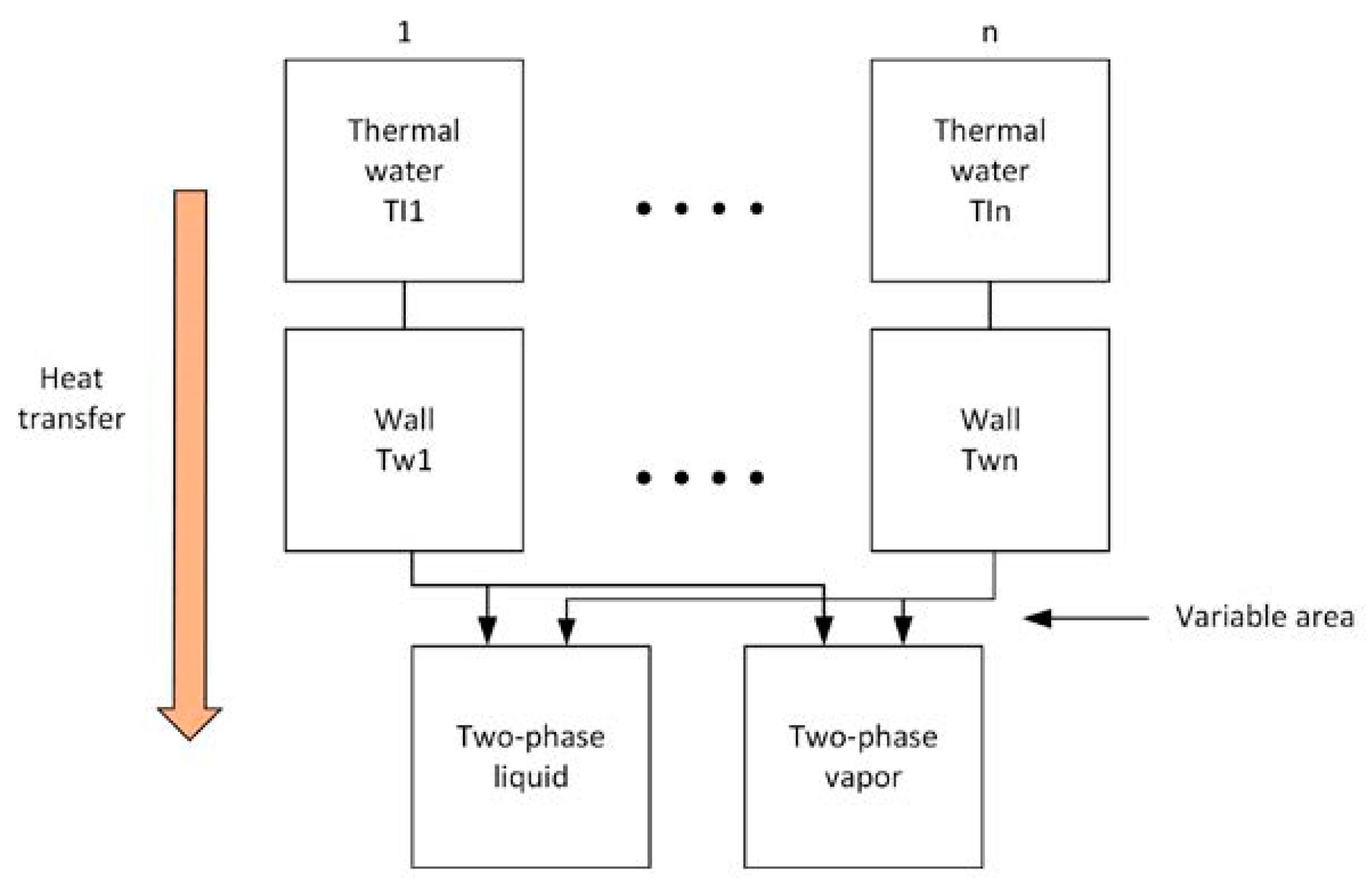
The heating fluid flows on the tube-side and vaporizes the organic fluid on the shell side. In this work, the tube-side pathway is discretized in a number of cells along its main flow direction, according to the FV method. Parallel tubes of the same pass are lumped in the same cells. Each cell is connected to a wall cell representing the solid material of the pipe, and transfers heat either to Region 1 or 2 (or a fraction of both) of the TVC, according to the liquid level and the position of the cell. The heat transfer scheme is shown in Figure 3. In general, the heat transferred by each cell can be written as:
where is the cell heat transfer coefficient, the cell heat transfer area, the cell temperature and the temperature of the tube wall at the cell side. The heat transfer between the wall cell and its interface with the cell is:
where is the average temperature of the wall and the thermal resistance of the wall cell. For the solid wall, the following dynamic equation is valid in each cell :
where is the specific heat capacity (for stainless steel assumed at 500 ), the density (for stainless steel assumed as ) and the volume of the wall cell. and refer to the heat transfer rate for the wall cell with the liquid and vapor volume. If the cell is completely submerged if it is completely exposed to the vapor . The heat transfer between the tube and the interface with Region 1 and/or 2 is:
where is the temperature of the wall at the interface with Region 1 and/or 2. The heat transferred by Region 1 with each single wall cell is described as:
where is the heat transfer coefficient of the evaporating liquid and is the external heat transfer area of the cell in contact with the liquid. The heat transferred by Region 2 with each wall cell is analogously:
where is the heat transfer coefficient of the vapor and is the external heat transfer area of the cell in contact with the vapor. The heating fluid considered in this paper is geothermal water. To compute the heat transfer coefficient , the equation proposed in McEagle [37] is used:
where is the liquid velocity inside the pipe and the internal diameter of the pipe. The McEagle correlation has been developed specifically for water and suggested by [37]. In absence of further information on the characteristics of the geothermal water, this correlation will be used.
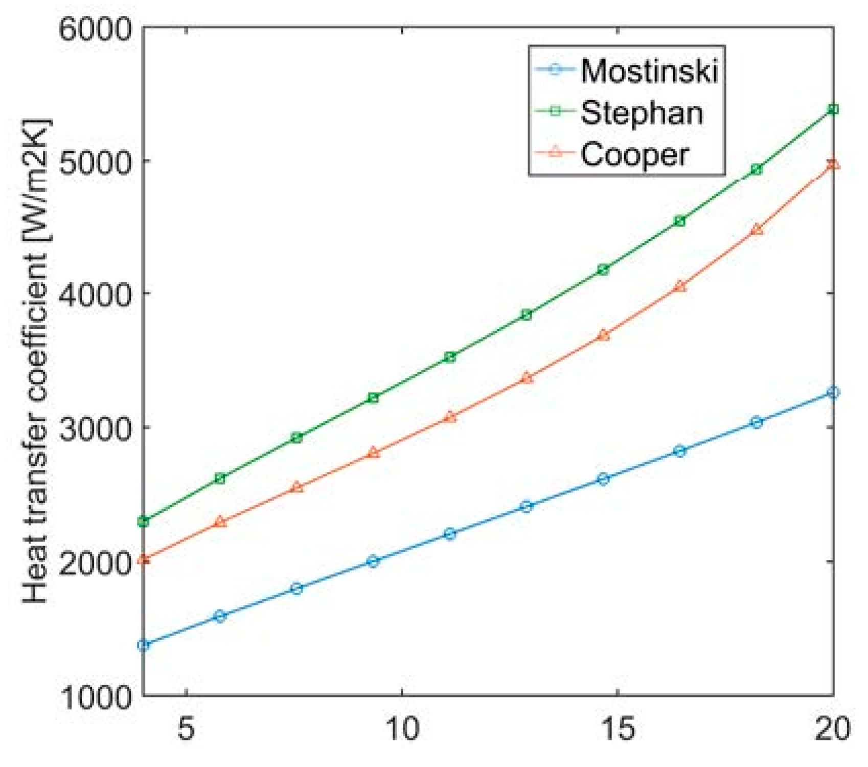
In a kettle boiler, the evaporation occurs in a quiescent pool of saturated liquid. The convective effects are in this situation almost negligible. The evaporation regime is called “nucleate boiling”, since the process takes place with the formation of bubbles, which detach when close to the vapor-liquid interface. The bubbles are generally formed in vapor filled cavities of rough tube surfaces [67]. A condition of stable nucleate boiling is given in [37], where a maximum heat flux at the tube bundle is defined. Since the heat transfer coefficient is dependent on the nature and condition of the heat exchange surface, a correlation with high accuracy for every system cannot be provided [37]. The heat transfer coefficient for pool or nucleate boiling can be described by means of several correlations. The Mostinski equation [68], which is a function of the cell heat flux and the pressure of the liquid, has a relative simple form:
where is the critical pressure of the fluid. The pressures have to be expressed in . Another proposed correlation, developed from statistical multiple regression techniques for organic fluids is the Stephan and Abdelsalam [69]:
where is the thermal conductivity and is the thermal diffusivity of the saturated liquid, is the saturation temperature and is the latent heat of vaporization at the pressure . The bubble departure diameter is defined as:
where is equal to 35° for every fluid and is the surface tension.
The Cooper equation is also function of the heat flux and liquid pressure [69]:
where is the pipe roughness in (for stainless steel ) and is the molecular weight of the organic fluid in .
The discussed correlations (23)–(26) for nucleate boiling are compared in Figure 4 for a common organic working fluid, in the range of pressures and heat flux equal to. Stainless steel is considered as pipe material. It can be seen that the Mostinski equation appears more conservative than the other two. The Cooper and Stephan equations show a very similar pattern, but the Stephan is slightly more conservative and has a more complex structure. Because of its simplicity, only the Cooper correlation is used in the following.
The film-boiling equation can be used for the heat transfer at cells that are not submerged under the liquid level and exchange heat with the vapor that surrounds them. The heat transfer is limited in this case by the conduction through the film of vapor and can be described by the Bromley equation [70]:
where is the thermal conductivity of the vapor, is the specific heat at constant pressure of the vapor, the external diameter of the pipe and the dynamic viscosity of the vapor.
The wall cell thermal resistance is defined as:
where is the tube internal diameter, is the tube thermal conductivity (for stainless steel assumed at 15 ), is the length of the wall cell and is the number of parallel tubes per pass.
2.3. Geometry of the Kettle Boiler
The kettle boiler used for the model validation is, according to the standards of the Tubular Exchanger Manufacturers Association, Inc. (TEMA) [71], of the type NKN with no baffles. The tube bundle extends horizontally for the entire heat exchanger and is welded to the shell in the front and rear side to form a box (for this reason, it is also called “box-type” [72]). As mentioned, the boiler has a freeboard used to vaporize the fluid on the shell side in subcritical conditions, and separate the liquid droplets that might be carried by the outgoing vapor stream itself. That is why such evaporator has a kettle diameter significantly bigger than the bundle one (usually one third larger than the inner bundle diameter). The bundle diameter is also called “shell diameter”. To minimize the amount of liquid extracted by the vapor flow, an impingement-type baffle is usually also present at the vapor outlet nozzle.
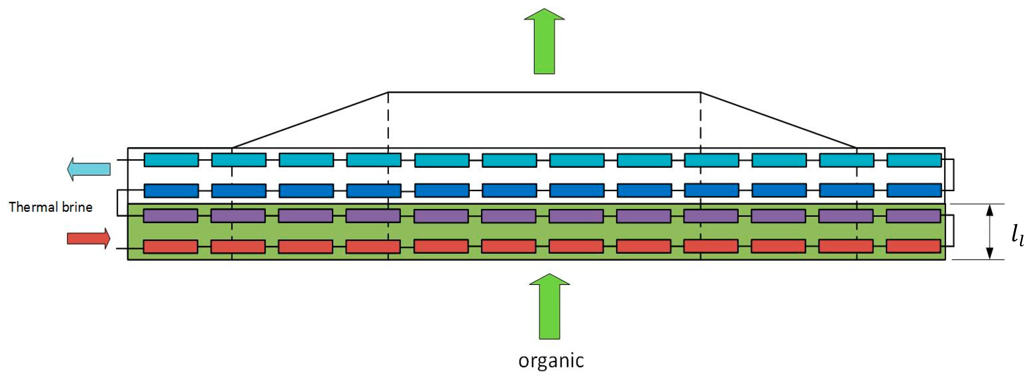
The geometry of the heat exchanger can be seen in Figure 5. The heating medium (for instance, geothermal water) flows inside the tubes, in a single or multi-pass arrangement. The tube path is discretized in cells to represent the model discretization discussed in Section 2.2. Parallel tubes of the same pass are lumped in the same cells. Figure 5 also shows the liquid and vapor volumes of the working fluid (resp. green and white regions). The flow directions are highlighted: the heating fluid (geothermal brine) enters and leaves the evaporator from the left, whereas the organic fluid enters the evaporator as liquid from the bottom and leaves it as vapor from the top.
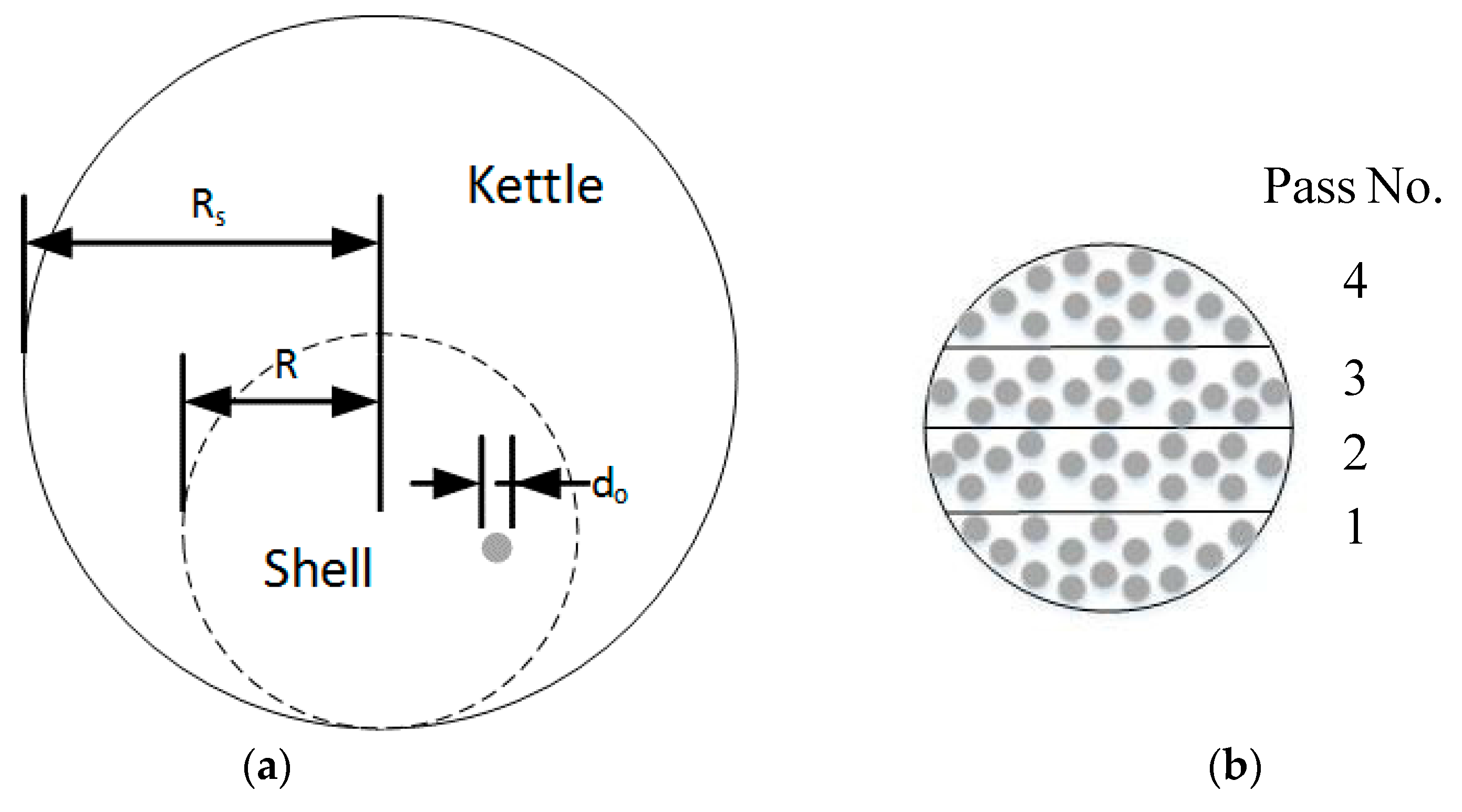
Region 1 and 2 occupy a larger or smaller volume according to the liquid level, and according to their volume, the tubes transfer more or less heat with each of the regions. To correlate the occupied volume by Region 1 and 2 with the liquid level, the geometry of the kettle boiler has to be defined. The cross-section of kettle boiler at the medium kettle length is shown in Figure 6. Different geometric parameters are defined in the following. The kettle is characterized by a kettle radius, corresponding to the largest internal diameter of the evaporator. The kettle has an internal shell (defined by the dash line in Figure 6a), characterized by a radius. The tube bundle is found within the shell. The bundle consists of a given number of tubes, having a certain outer diameter, a wall thickness and length. As an example, the cross-section of a single tube is shown in grey in Figure 6a. The shell is redrawn in Figure 6b together with the tube bundle (in grey) and subdivided in four segments, representing four tube passes. The cross-sectional area occupied by the tube bundle over the shell is (grey area of Figure 6b):
The remaining free cross-sectional area of the shell is (white area of Figure 6b):
An important quantity is the ratio of the free cross-sectional area of the shell (white area of Figure 6b) to total cross-sectional area of the shell (white plus grey area of Figure 6b):
The larger, the larger the volume available for the working fluid on the shell side. In a first approximation, it can be assumed that the local, i.e., the area ratio considering only a portion of the shell, is uniform and equal to the shell of Equation (31). As mentioned, the tube-side flow can be arranged in multiple passes . The inner diameter of each tube is . The heat transfer area for each tube cell from the inner side (used in Equation (16)) is:
For each pass, the cross-sectional area of the tube bundle is:
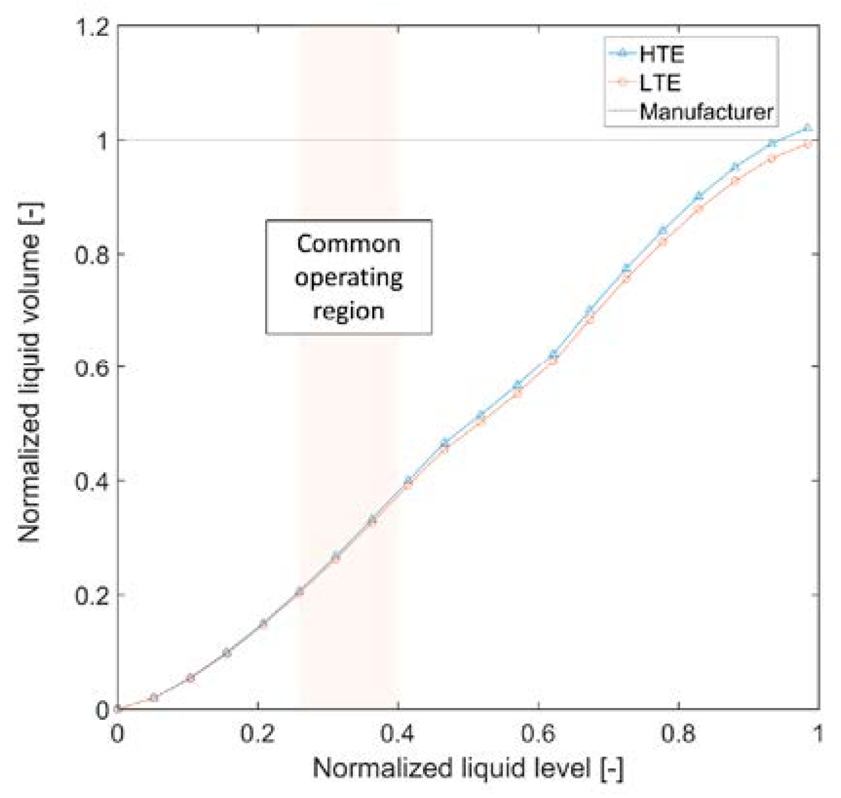
The equations that relate the liquid volume in the evaporator and the liquid level are defined in Appendix B and the results from Equation (A23) are plotted in Figure 7 for two kettle evaporators. The evaporators are located in an ORC geothermal power plant in Sauerlach, Germany (see Section 3.1). For confidentiality issues, the quantities have been normalized to the manufacturer data. The discrepancy between the proposed volume method and the values given by the manufacturer is shown in Table 1. The errors are 2.29% and −0.37% for the two evaporators.
3. Validation and Results
In this section, the model of the evaporator is validated and compared with available measurements from the geothermal power plant in Sauerlach. Section 3.1 describes the power plant configuration and which measurements are available. The simulation set-up is compared in Section 3.2. In Section 3.3 the case studies are described and the results are shown in Section 3.4.
3.1. Geothermal CHP Plant in Sauerlach
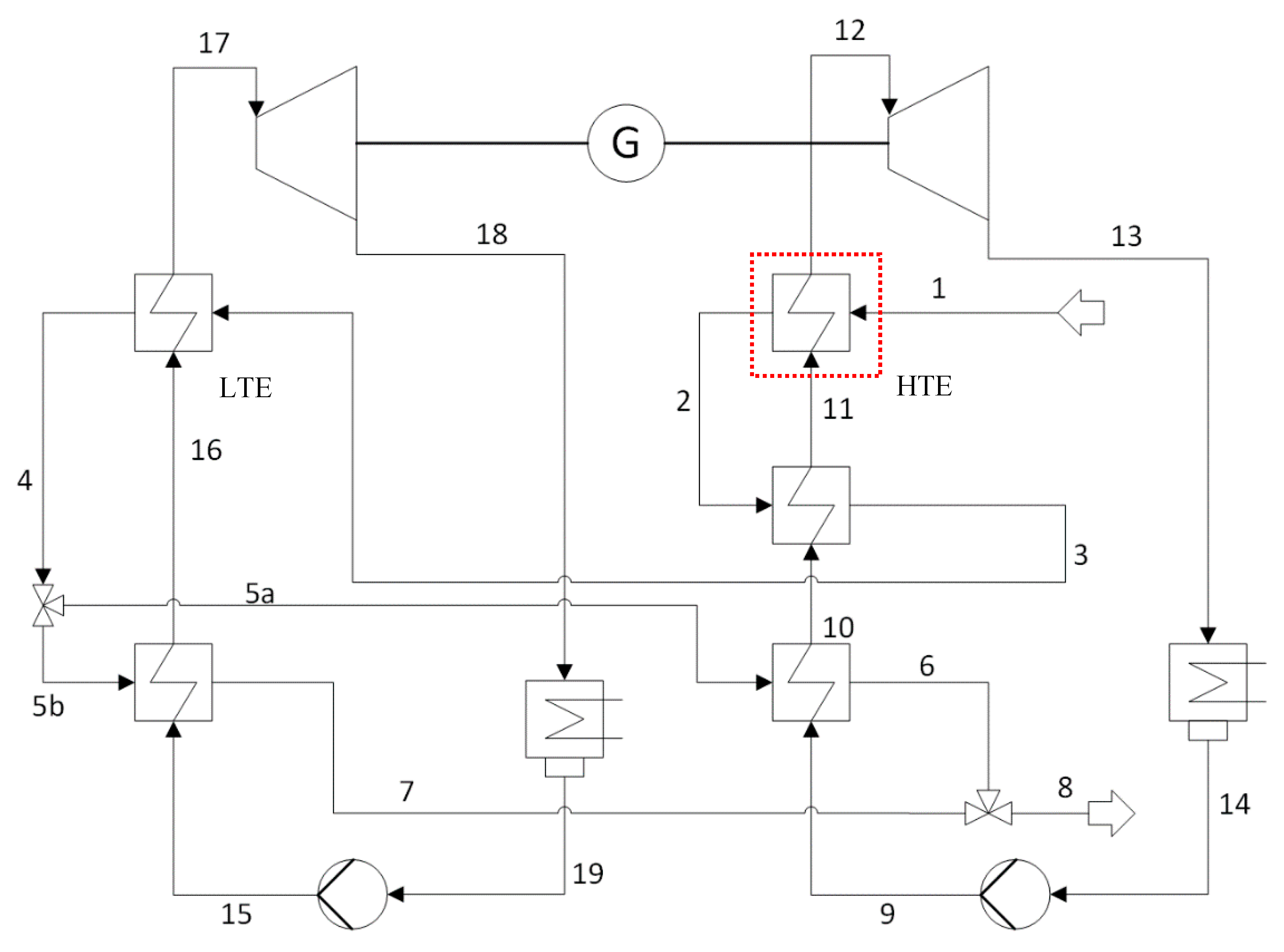
The geothermal power plant in Sauerlach is one of the largest geothermal power plants in Germany, with an electrical output of approximately 5 MWe and a thermal output of around 4 MWth. The plant has 10.99% of net electrical efficiency. At the design point, the geothermal brine has a temperature of 140 °C, a nominal volume flow rate of 110 L/s. The plant configuration is depicted in Figure 8.
The plant consists of a dual-pressure ORC that makes use of the split concept [73]. The high temperature (HT, or high-pressure) cycle has one evaporator and two preheaters. The low temperature (LT, or low-pressure) loop has one evaporator and one preheater. The thermal water is pumped from the extraction probe (1) to the high temperature evaporator (HTE), and then flows to the high temperature preheater of the high temperature cycle (2 → 3). At this point the still hot thermal brine is fed to the low temperature evaporator (3 → 4). Then the flow is split into lines (5a) and (5b) that go respectively to the low temperature preheater of the high temperature cycle and the only preheater of the low temperature loop. After being cooled down to around 45 °C in (6) and (7) the thermal water is fed back to the injection probes at point 8. The HT cycle and the LT cycle are completely separated in terms of organic fluid process. The high and low temperature condensers are air-cooled, by means of induced-draught fans. The condensate from the air cooled condensers is then collected in the condensate tanks, from which the pump drives the liquid back to the preheaters (14 → 9 and 19 → 15). The turbines are connected via a gearbox to a single synchronous generator, since they have different rotational speed (around 2683 and 1457 rpm for the HT and LT turbines respectively). They are single-stage axial turbines. In the start-up phase, a bypass valve controls the flow passing through each turbine. The plant is in fact a CHP plant. Different bypass valves are available through the thermal water pathway, to allow a proper control of the heat and electrical load. In particular, an extraction for the district heating system is placed at point 3, but also a bypass directly at point 1 can be used. In this way a combination of parallel and series (at least in a small portion) configuration of the power and the heat production systems is achieved, which guarantees more flexibility.
The present work focuses on the HTE (in red box in Figure 8). The measurement available for the thermal brine are the volume flow rate and the pressure at point 1 and the temperatures at points 1 and 2. For the organic fluid, the temperatures at points 11 and 12 and the pressure in the evaporator (ca. 12). The volume flow rate of organic fluid is measured at the outlet of the pump (point 9). By means of the temperature at point 14 and pressure at point 9, the mass flow rate is computed. Since between points 9–11 the organic fluid is at the liquid phase, the mass flow rate at the HTE inlet is assumed equal to the one at the pump outlet. A summary of the available measurements is provided in Table 2.
3.2. Simulation Set-Up
The model of the kettle boiler is simulated in Dymola. The standard solver DASSL is used, with tolerance. The model has been developed combining present models of the TIL library (heating fluid and wall cell) and creating a new TVC model (see Section 2). The fluid properties are computed by means of REFPROP. The model has been assembled in a single component called “KettleBoiler”.
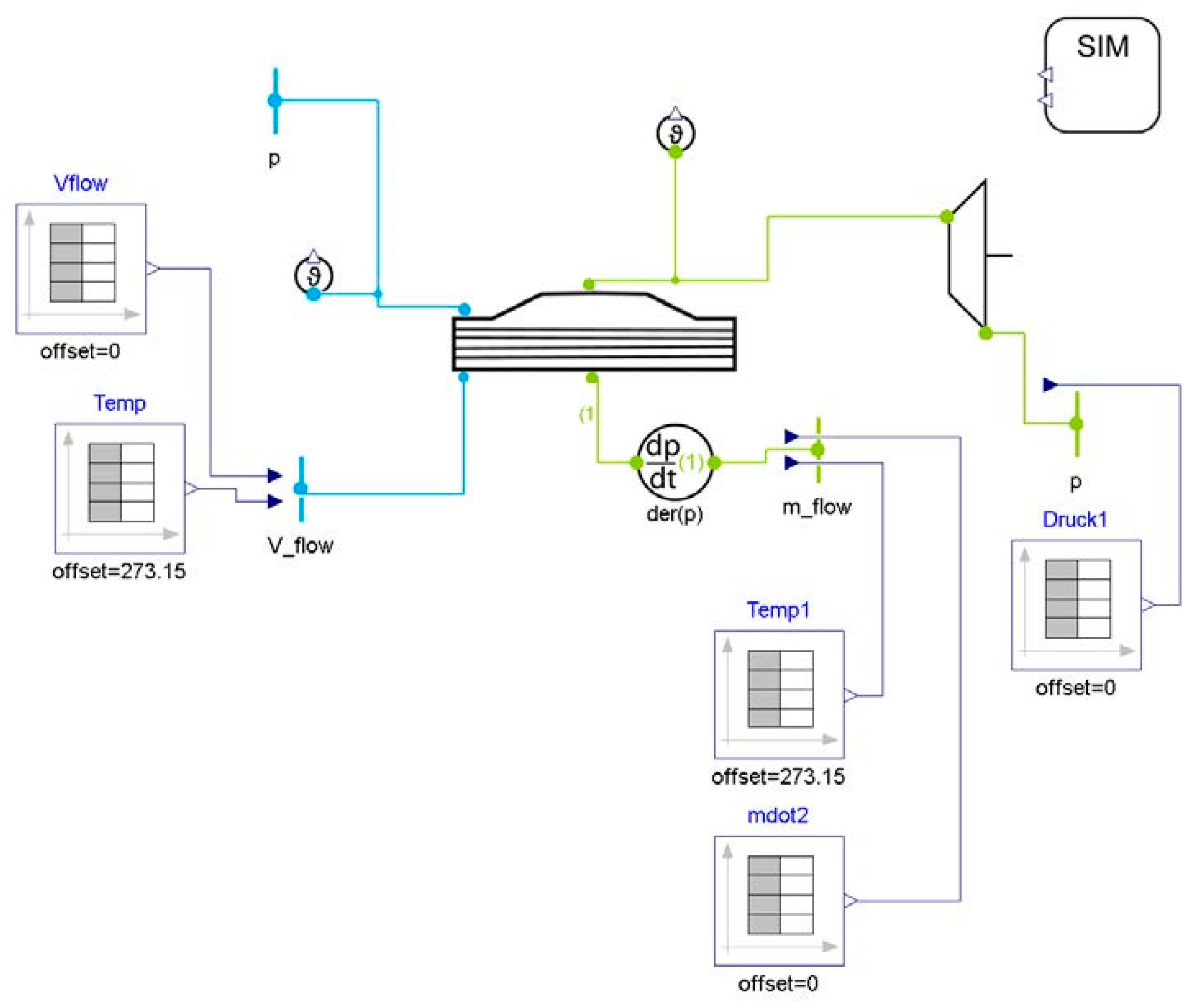
The main geometric features of the boiler, the initial states of both fluids and some other settings that can be modified are summarized in Table 3. The reference vapor qualities for evaporation and condensation are set at resp. and for numeric reasons. Both mass transfer coefficients and are set at, as the impact of these parameters is limited and the set values could guarantee a best match for the simulation. The pressure drops at the nozzles and in Equations (9)–(11) are neglected. Since the pressure difference between the top and the bottom of the liquid level is lower than 0.5% the absolute pressure, it is assumed that The simulation set-up is shown in Figure 9. The blue line refers to the thermal brine and the green to the organic fluid. The inlet thermal flow rate and temperature of the thermal brine are set as measured. For simplicity, its pressure is fixed at 10 bar. For the organic fluid the inlet temperature is set as measured. The mass flow rate at the inlet is set as the calculated mass flow rate for the pump outlet. The evaporator is connected to a turbine, modelled through the common Stodola’s equation:
where is the turbine pressure ratio and is the turbine characteristics. The outlet pressure of the turbine is also set as measured. The pressure and liquid level in the evaporator, together with the HTE outlet temperatures for both fluids are therefore a result of the simulation.
3.3. Case Studies
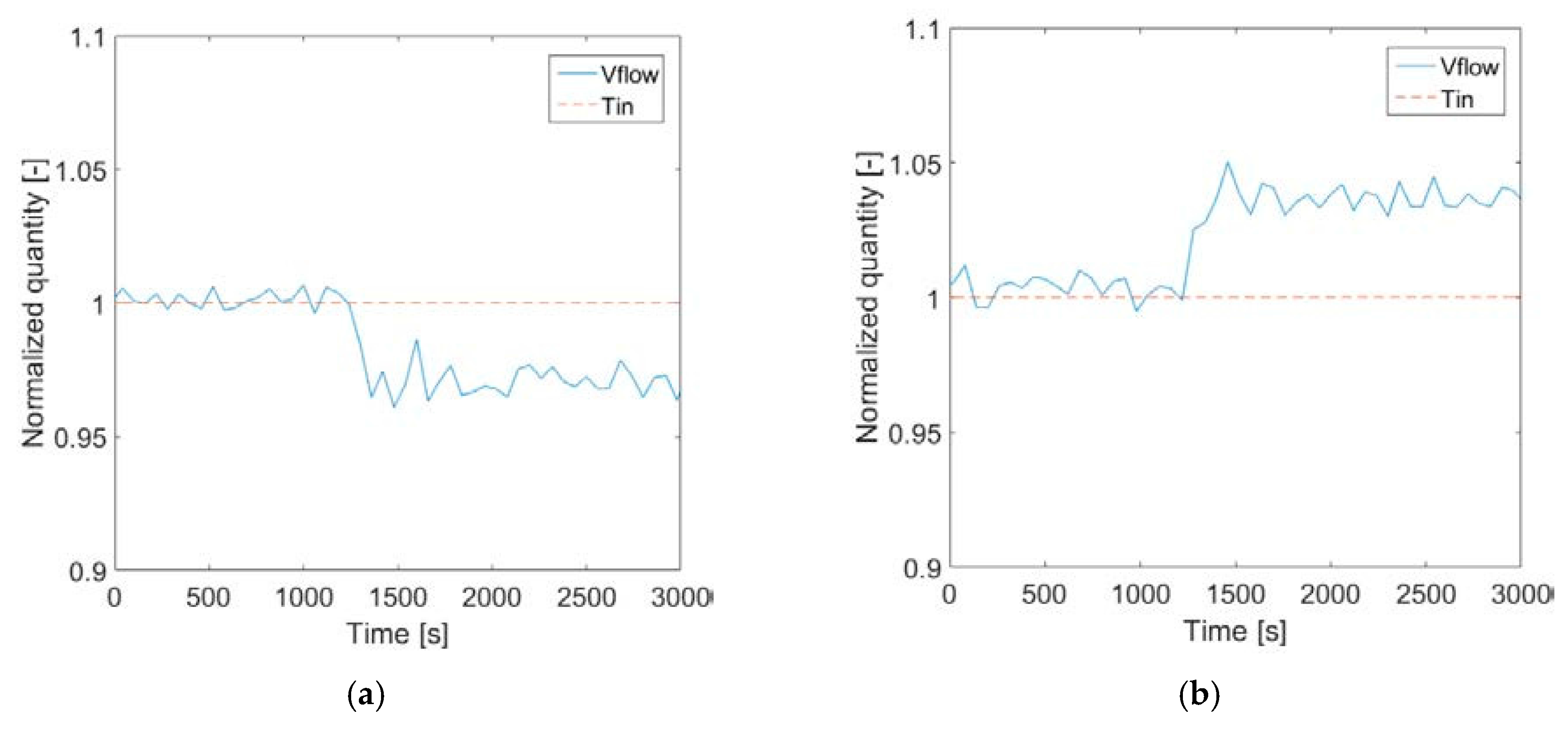
Two case studies are evaluated for the validation of the evaporator model, based on measurement data from Sauerlach. Case 1 refers to measurements taken on 23 May 2015, whereas Case 2 refers to measurements taken on 14 May 2015. A step function in inlet volume flow rate of thermal brine is applied in both cases: in Case 1, the step is negative and has an amplitude of 2.98%, whereas in Case 2 the volume flow rate is increased by 3.26%. The two measured profiles are shown in Figure 10. The values have been normalized for confidentiality issues. It can be seen that the inlet temperature of the geothermal brine does not vary significantly, as it commonly is in deep geothermal power plants.
3.4. Simulation Results
The simulation is run separately for the two cases since the boundary conditions are different. All the values except the time scale have been normalized for confidentiality issues. The boiler operates in regime of stable nucleate boiling (mentioned in Section 2.2), given the limited temperature difference and the heat flux at around 50% of the critical heat flux.
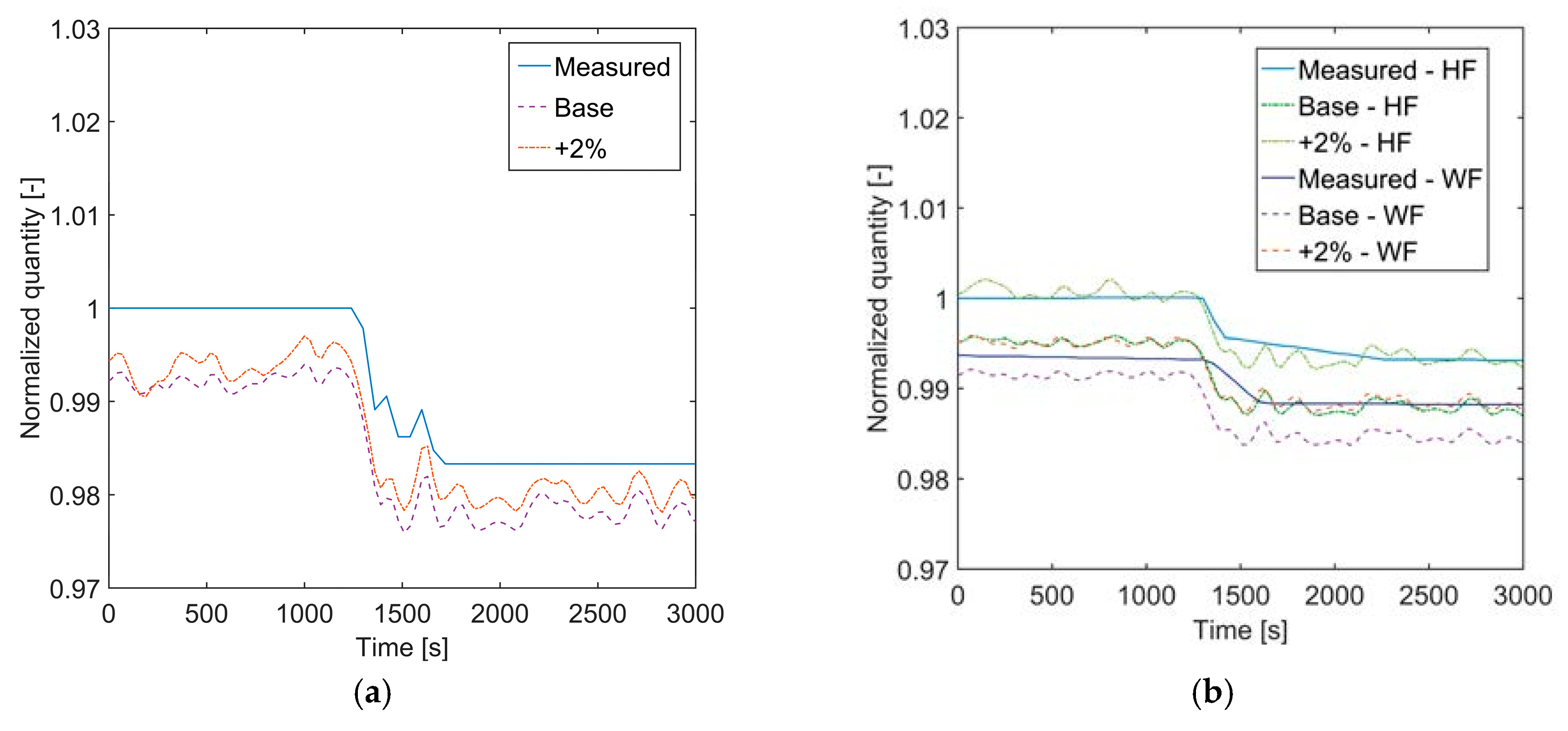
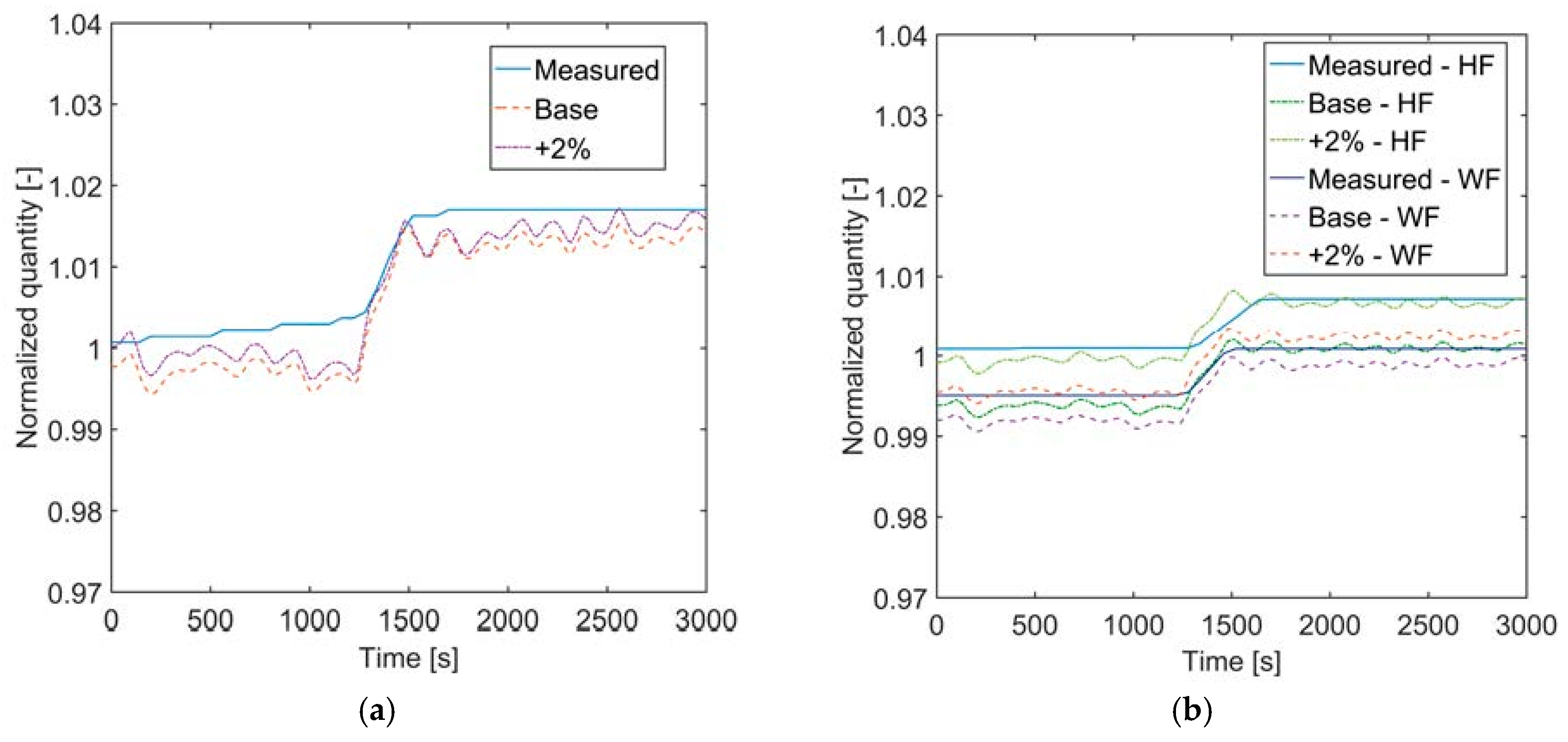
In Case 1, the drop in thermal brine volume flow rate at (see Figure 10a) causes a drop in the measured pressure of approximately 1.5%, as shown in Figure 11a (“Measured” line). The same drop is represented in the simulation, which has a starting offset of 0.9% (“Base” line) that is however kept over the entire simulation, so that the error remains within 1% for the entire simulation. The outlet temperature of the working fluid (WF) and of the thermal brine (HF) are lower than measured, even though within 1% (“Base” line in Figure 11b). In Case 2, the change in pressure is opposite to Case 1, and increases of 1.7% (“Measured” line in Figure 12a).
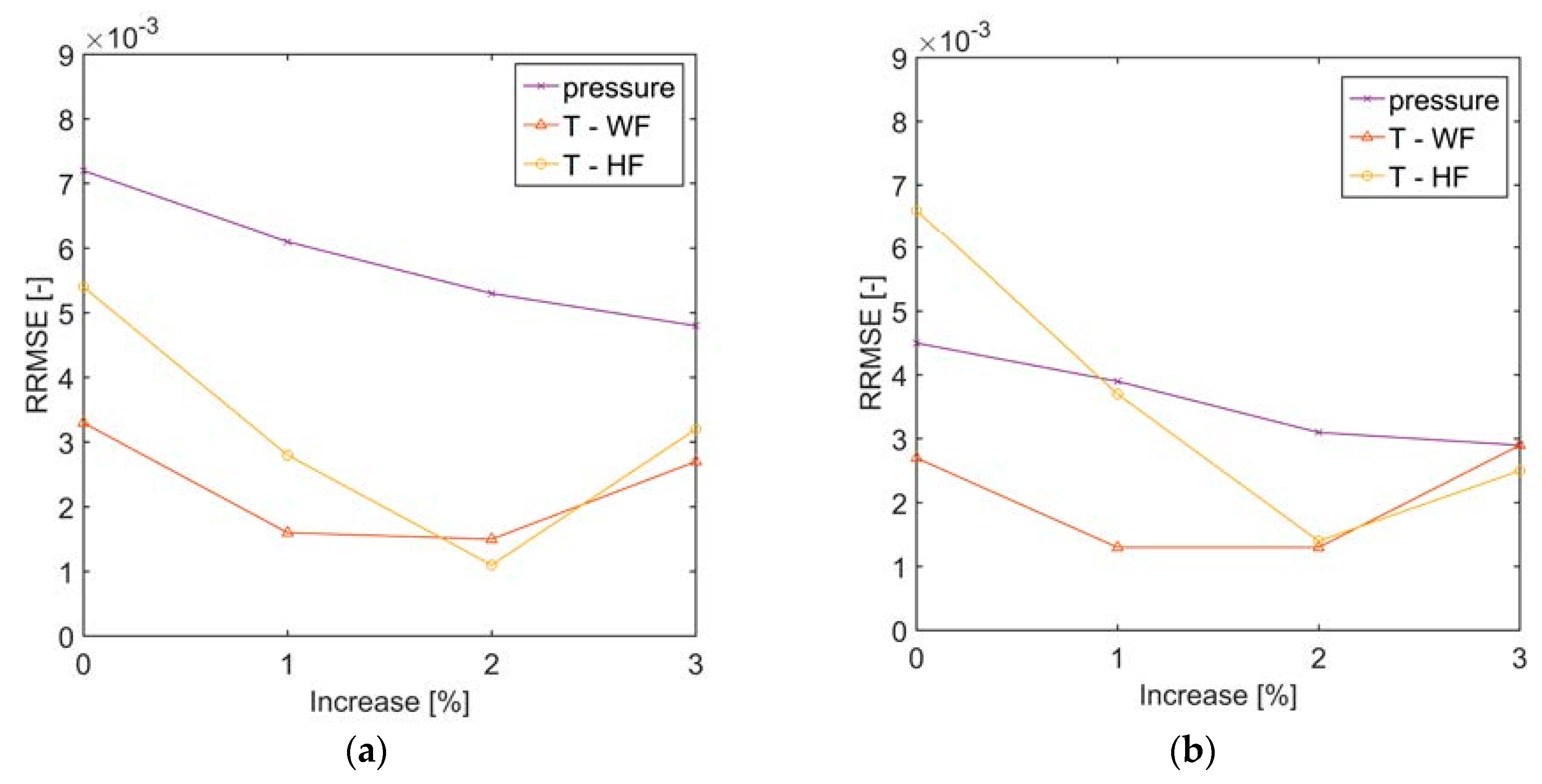
The simulation follows the same pattern, even though an offset lower than 1% is observable (“Base” line). The outlet temperature of both fluids follow the measured value within a 1% difference (cf. “Measured” and “Base” line in Figure 12b). A sensitivity analysis on the effect of the increase in volume flow rate of thermal water is carried out and shown in Figure 13. To account for differences between measurement and simulation over the entire simulation time, the relative root mean square error RRMSE is considered:
where is the number of time intervals, is the measured value and is the respective simulated value. Figure 13 shows that an increase of 2% of volume flow rate of thermal brine leads to the minimum RRMSE in temperature. In fact, by increasing the thermal brine volume flow rate of 2% over the entire simulation, the RRMSE for the outlet temperatures goes below 0.2% in both Cases 1 and 2. The time behavior in pressure and temperature with the 2% increase in thermal brine volume flow rate can be observed in the “+2%” line in respectively Figure 11 and Figure 12.
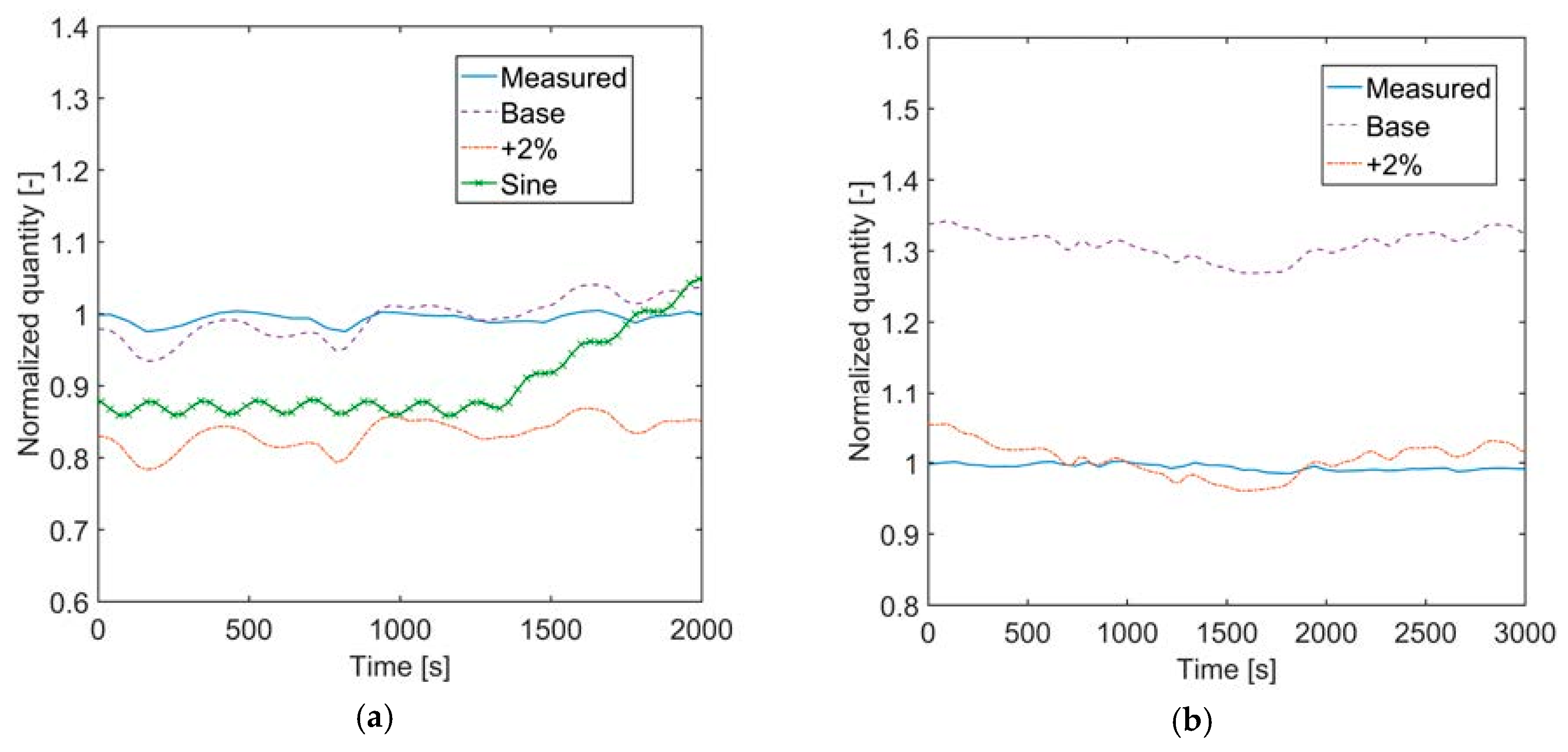
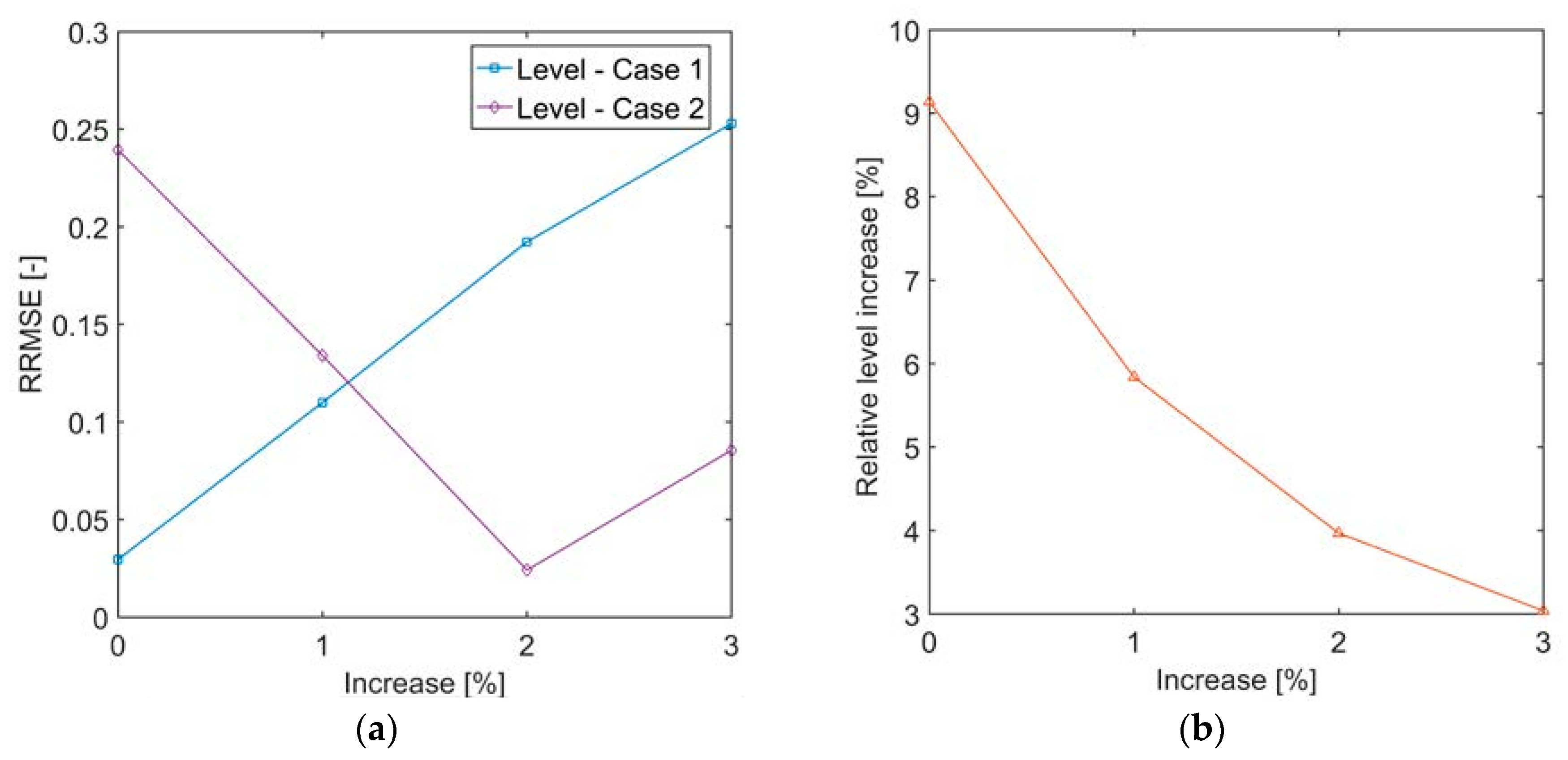
Figure 14 shows the measured and simulated liquid level in Cases 1 and 2. It can be seen that the agreement is not as accurate as for pressure and temperatures. In Case 1, the simulated level shows an offset below 5% relative to the measured data (cf. “Measured” and “Base” line in Figure 14a). When the flow rate of thermal brine is increased by 2% over the entire simulation (“+2%” line), the offset becomes negative. Referring to the maximum level (i.e., evaporator full of liquid), the difference from the measured value remains below 3% in the “Base” line and within −7% in the “+2%” line. In Case 2 (Figure 14b), the offset in the “Base” line is larger than in Case 1, but it is reduced to less than 10% (relative to the measured value) when the thermal water flow rate is increased by 2% (“+2%” line). Referring to the maximum evaporator level, the differences are lower than 12% in the “Base” line and 2% in the “+2%” line. The effect of the increase in volume flow rate of thermal brine on the RRMSE for the evaporator liquid level is depicted in Figure 15a. In Case 1, the offset would be minimum for no increase of thermal brine volume flow rate, whereas for Case 2 the increase should be around 2%.
From Figure 14a, a growing tendency in simulated evaporator level over time can be observed (“Base” line), which does not appear in the measured value (“Measured” line). The growing tendency is made noticeable by the significant simulation time (), and analyzed in Figure 15b, where the level increase in the simulation over the average value of the measured level is shown. The level increase drops as the volume flow rate of thermal brine is increased. The effect can also be seen by comparing the “Base” and “+2%” line in Figure 14a. The difference becomes even smaller for higher volume flow rate of thermal brine. The growing tendency of the liquid level in Case 1 seems to be generated by a non-sufficiently accurate inlet mass flow rate of organic fluid in the evaporator.
This quantity was in fact approximated as the product of the volume flow rate measured at the pump outlet and the density computed from the measured pressure at the pump outlet and the temperature before the pump. In addition to this, the measured data are available only at a minute sampling time between two consecutive measurements. As an example, Figure 14a shows the liquid level in the evaporator (“Sine” line), when this is subjected to a sinusoidal inlet mass flow rate of organic fluid oscillating around the same average value as the measured one for , with a period of 180 s and an amplitude of 2 kg/s. The liquid level also oscillates around an average value, with no growing tendency. This confirms the hypothesis of the influence of inaccuracies on the inlet flow rate of the organic fluid on the growing trend for the liquid level. For, the liquid level suddenly increases because of the negative step in volume flow rate of thermal brine (Figure 10a), which can no longer lead to evaporation of the same amount of organic fluid. If the inlet mass flow rate of organic fluid continues to sinusoidally oscillate around the same average value and the evaporation rate drops, the liquid level grows as shown in Figure 14a.
4. Discussion
In the present analysis, a dynamic model of a kettle boiler was developed in Modelica® language, by partially making use of models provided by the TIL-library and partially creating new components or features. The boiler model can be effectively useful for larger scale ORC plants, where kettle boilers are very often applied. The model was tested against available measurements from a geothermal CHP plant in Sauerlach, Germany. The pressure of the organic fluid and the outlet temperatures of both organic and heating fluid could be reproduced within a 1% error in case of a negative (Case 1) or positive (Case 2) step change in inlet volume flow rate of the heating fluid.
In Section 3, the pressure difference between top and bottom of the liquid volume in the evaporator was neglected. The assumption of negligible pressure difference in the liquid level is justified by the fact that the pressure difference is typically below 0.5% of the absolute pressure at the top of the volume. Nevertheless, if such pressure difference is considered, no significant pressure and temperature difference of the vapor is found. The average pressure in the liquid volume would be slightly higher because of the liquid column, and this can lead to a variation of liquid level to 2% with respect to the simplified case. The heat transfer coefficient for pool nucleate boiling (with the Cooper correlation) increases by less than 1%.
The accuracy on the liquid level in the evaporator could not in general be as high as for the evaporator pressure and outlet temperatures. In the attempt to explain the reasons for the liquid level offset (and the improved temperature matching) when increasing the thermal water flow rate by 2% over the entire simulation time, the fluid properties of the thermal water and the working fluid were analyzed, but no clear explanation through these parameters could be found. It might be assumed that the improvement achieved by increasing the volume flow rate of thermal brine could be caused by a deviation in latent heat of vaporization for the working fluid. If the volume flow rate of thermal brine is increased and the amount of working fluid that evaporates does not change, the latent heat of vaporization of the working fluid should be higher in the simulation than in the real case. Using the Peng-Robinson equation instead of REFPROP, the calculated heat of vaporization becomes even smaller, in contrast with the hypothesis. Future work should focus on analyzing the working fluid used in Sauerlach and comparing to the REFPROP database to gain major information on the differences in fluid properties.
Because of its simplicity and better agreement with the results, the Cooper correlation was used in this work. The Stephan and Mostinski correlations (Equations (23) and (24)) would lead to a higher liquid level because the lower heat transfer coefficient requires a higher heat transfer area to vaporize the same amount of fluid.
5. Summary and Conclusions
Dynamic simulations of ORC systems have been recently gaining significant interest. A dynamic model of a kettle boiler was presented in this paper. The model was developed as a combination of a discretized finite volume method on the tube side, and two volumes in non-equilibrium for the evaporating fluid on the shell side. The simulation results were compared to measurements available from a geothermal CHP plant in Sauerlach, Germany. Two cases were investigated: one case where the evaporator undergoes a negative step variation in inlet volume flow rate of thermal brine, and one case where a positive step variation is instead applied. The boundary conditions were set as measured. The simulation results showed a good agreement with the measurements, for what regards the evaporator pressure and outlet temperatures of the working and heating fluids. An increase in 2% of the inlet volume flow rate of the heating fluid over the entire simulation could lead to a better agreement with the temperature measurements. The liquid level was the most challenging quantity to compare, because of measurement uncertainties and possible discrepancies in fluid properties. The model can reproduce with high calculation speed the dynamic behavior of the kettle boiler, keeping the error in pressure and outlet temperatures below 1%. The model offers a high flexibility in geometry of the heat exchanger, being able to handle a multi-pass scheme. It can be implemented for future cycle optimization, in both design and off-design conditions. In future work, the entire cycle in Sauerlach will be simulated, and validated with additional measurements. The fluid properties should also be analyzed more thoroughly. As a result of the simulations, solution for an improved dynamics and control of the power plant will be proposed. The results will be valid not only for the power plant in Sauerlach, but also for other similar power plants.
Acknowledgments
The authors would like to thank the company Stadtwerke München (SWM) for the support and the information provided for the development of the present paper. The present work was funded by the Geothermie-Allianz Bayern (GAB) and the Munich School of Engineering (MSE) of the Technical University of Munich (TUM). This work was supported by the German Research Foundation (DFG) and the Technical University of Munich (TUM) in the framework of the Open Access Publishing Program.
Author Contributions
Roberto Pili is the main developer of this work. Christoph Wieland substantially contributed to the development of the idea, to the discussion of the results and to the final manuscript. Hartmut Spliethoff supervised the work and its development.
Conflicts of Interest
The authors declare no conflict of interest. The funding sponsors had no role in the design of the study; in the collection, analyses, or interpretation of data; in the writing of the manuscript, and in the decision to publish the results.
Abbreviations
| CFD | Computational fluid dynamics |
| CHP | Combined heat and power |
| DAE | Different-algebraic equation |
| FEM | Finite element method |
| FV | Finite volume |
| HF | Heating fluid (geothermal brine) |
| HT | High temperature (and pressure) cycle |
| HTE | High temperature evaporator |
| ORC | Organic Rankine Cycle |
| LT | Low temperature (and pressure) cycle |
| LTE | Low temperature evaporator |
| MB | Moving boundary |
| RRMSE | Relative root mean square error |
| TV | Two volumes |
| TVC | Two-volume cavity |
| SWM | Stadtwerke München (Company) |
| WF | Working fluid (organic fluid) |
Variables
| Heat transfer rate | (W) | |
| Specific heat at constant pressure | (J/kgK) | |
| Mass flow rate | (kg/s) | |
| Slope of the conic section | (m) | |
| Heat flux | (W/m2K) | |
| Wall thickness | (m) | |
| Fractional area | (-) | |
| Axial position for j-th element | (m) | |
| Latent heat of evaporation | (J/kg) | |
| Pressure drop | (Pa) | |
| Specific enthalpy | (J/kg) | |
| Heat transfer area | (m2) | |
| Mass transfer coefficient | (s−1) | |
| Axial length | (m) | |
| Numberof passes or samples | (-) | |
| Radius | (m) | |
| Temperature | (K) | |
| Volume | (m3) | |
| Diameter | (m) | |
| Radius increment | (m) | |
| Axial length increment | (m) | |
| Acceleration of gravity | (m/s2) | |
| Level | (m) | |
| Mass | (kg) | |
| Number of tubes per pass | (m) | |
| Pressure | (Pa) | |
| Time | (s) | |
| Flow velocity | (m/s) | |
| Steam quality | (-) |
Subscripts
| in | Inlet |
| out | Outlet |
| l | Liquid volume |
| v | Vapor volume |
| evap | Evaporation |
| cond | Condensation |
| sat | Saturation |
| cell | Cell |
| i | Inner/inside tube |
| o | Outer/shell side |
| c | Critical point |
| s | Shell |
| cs | Cross section |
| cylind | Cylindrical section |
| sat | Saturation |
Greek letters
| ρ | Density | (kg/m3) |
| γ | Void fraction | (-) |
| α | Heat transfer coefficient | (W/m2K) |
| λ | Thermal conductivity | (W/mK) |
| η | Dynamic viscosity | (Pa s) |
| σ | Tube/Shell cross-sectional ratio | (-) |
Appendix A
The contact areas and of each wall cell with the two TVC is computed as described in this section. Each pass (or segment) has a certain cross-sectional area as defined by Equations (33) and (34). Another useful quantity is the cross-sectional area of the tube bundle in contact with the liquid volumefunction of the liquid level . The relationshipis determined as follows, for:
In Modelica®, the function is critical during the iteration procedure for the solver. Very often, the solver tries to find a solution out of the function validity range ±1. To solve the problem, a function called ComputeAl is defined during the initialization procedure, which computes the tube wet area for a finite number of levels, so that during the simulation procedure the solver interpolates among the previously computed points. Since the Modelica® function Modelica Math Vectors Interpolate requires monotonic increasing functions, the condition A2 is modified with a slightly increasing value as, for:
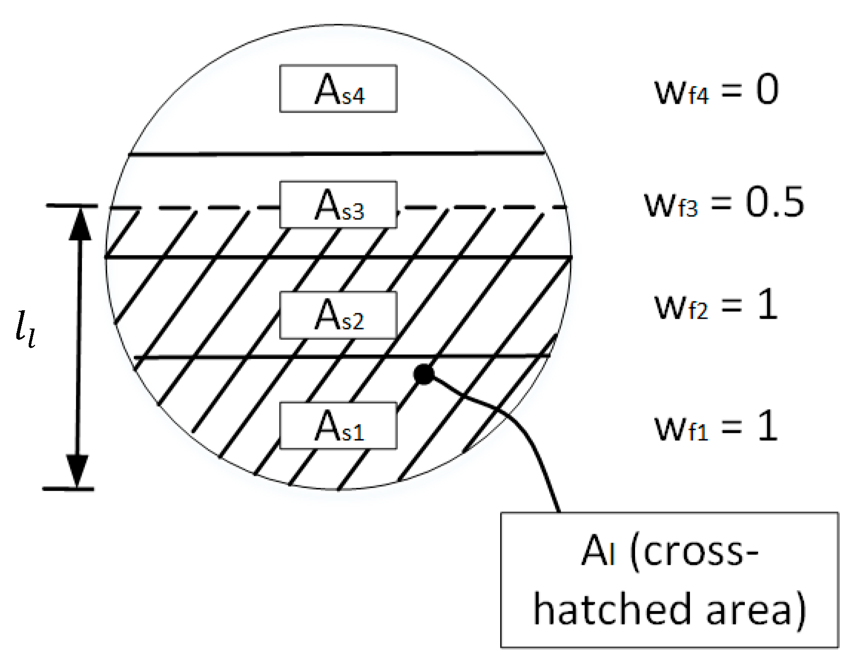
At this point, to recognize which portion of each pass is under or above the liquid level, the area fraction in each pass is defined:
When, the pass is completely submerged, when it is completely dry. If only partially submerged, the pass has. It is clear, that all cells of the same pass have the same area fraction. In addition, when a pass is partially or completely submerged, all previous passes must be completely submerged, i.e., for. The concept is illustrated in Figure A1. Attention must be paid to the fact that in this figure the cross-sectional area of each pass and the submerged area refer only to the tube cross-sectional area. In other words, the free cross-sectional area of the shell (white area of Figure 6b) is excluded.
Given the pipe submerged fraction, the transfer area for a tube cell with the liquid can be computed. For a discretization of each pass into, given the length of the single pipe and given pipes per pass, the ratio of the heat transfer surface with respect to the fluid cross-sectional area for the i-th cell in the pass is:
Therefore, the heat transfer area with the liquid volume for the i-th cell of pass is:
and for the vapor volume:
Figure A1.
Cross-sectional areas and area fractions as a function of the liquid level (all areas here shown refer to only the cross-sectional area of the pipes).
Figure A1.
Cross-sectional areas and area fractions as a function of the liquid level (all areas here shown refer to only the cross-sectional area of the pipes).

Appendix B
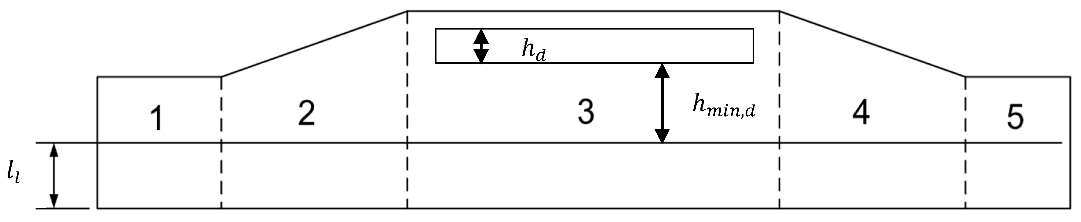
To compute the liquid volume as a function of the liquid level , the evaporator is divided axially in 5 regions, as shown in Figure A2. The internal and external regions are cylindrical, and the two regions in between (2 and 4) are conic, with inclined axis, since the bottom line follows the horizontal plane of the ground where the evaporator is mounted.
For the cylindrical regions, the following areas are defined:
And, with the kettle inner radius:
The liquid volume of regions 1 and 5, each of the length, is:
For the liquid volume of region 3, a demister at the top of the kettle has to be considered (Figure A2):
where is the demister volume.
The liquid volume of region 3, given the length , becomes:
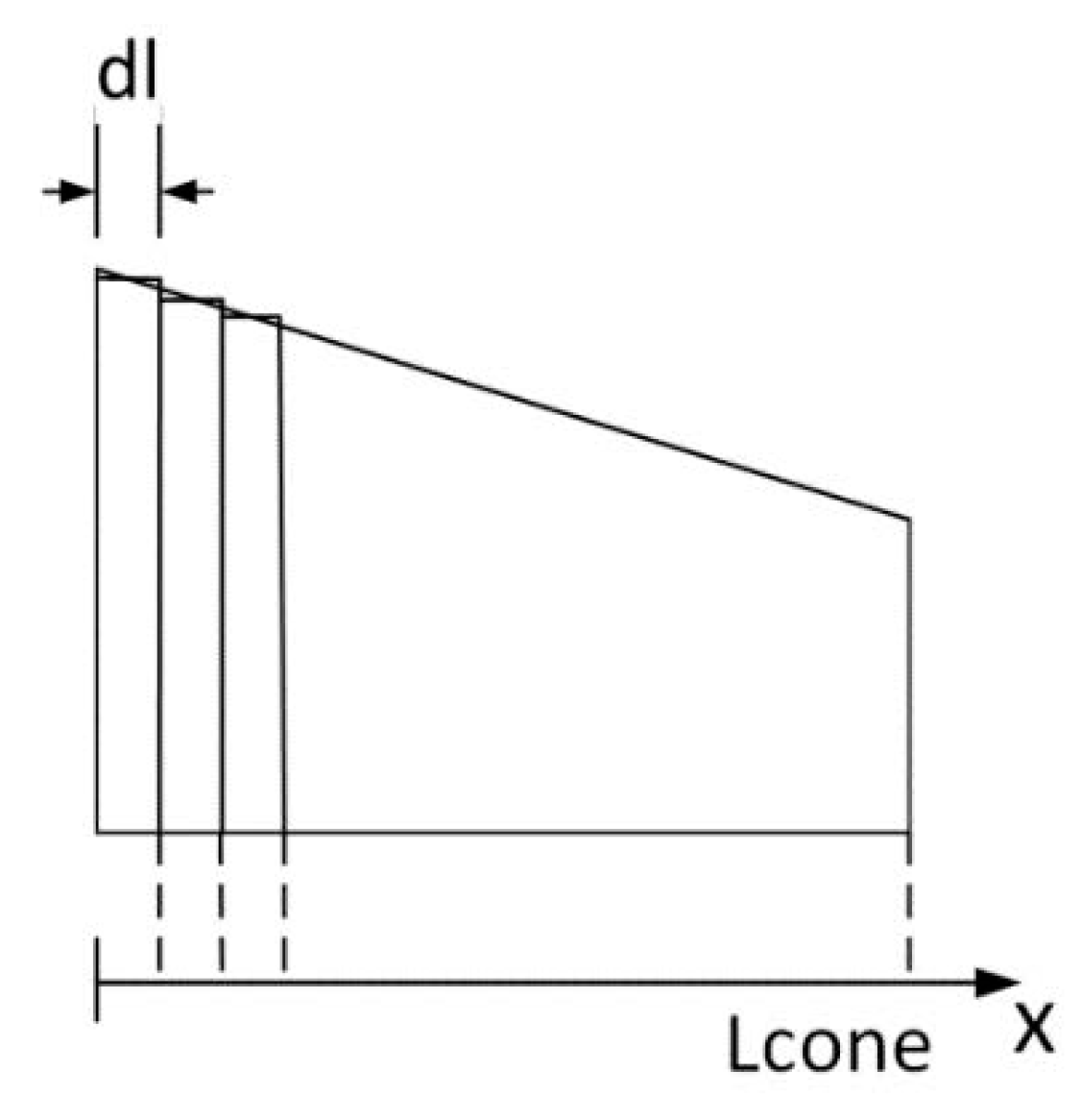
For the conic regions 2 and 4, each cone of length is subdivided axially in N cylinders of equal length (see Figure A3):
Fixing an x-axis on the horizontal bottom line of the cone starting from the end of bigger radius, the position of each sub-cylinder is:
Figure A2.
Discretization of the evaporator for liquid volume-level computation.

Given the slope of the upper side of the cone as:
The radius of each cylinder is:
In this way, the volume of each small cylinder is computed as for regions 1, 3 and 5, substituting the radius or with:
The volume of the conic region is therefore:
The liquid volume as a function of the liquid level is therefore:
Figure A3.
Discretization of the conic region.

References
- Tartière, T. ORC Market: A World Overview. Available online: http://orc-world-map.org/analysis.html (accessed on 16 August 2016).
- Schuster, A.; Karellas, S.; Kakaras, E.; Spliethoff, H. Energetic and economic investigation of Organic Rankine Cycle applications. Appl. Therm. Eng. 2009, 29, 1809–1817. [Google Scholar] [CrossRef]
- Tchanche, B.F.; Lambrinos, G.; Frangoudakis, A.; Papadakis, G. Low-grade heat conversion into power using organic Rankine cycles—A review of various applications. Renew. Sustain. Energy Rev. 2011, 15, 3963–3979. [Google Scholar] [CrossRef]
- Quoilin, S.; van Den Broek, M.; Declaye, S.; Dewallef, P.; Lemort, V. Techno-economic survey of Organic Rankine Cycle (ORC) systems. Renew. Sustain. Energy Rev. 2013, 22, 168–186. [Google Scholar] [CrossRef]
- Colonna, P.; Casati, E.; Trapp, C.; Mathijssen, T.; Larjola, J.; Turunen-Saaresti, T.; Uusitalo, A. Organic rankine cycle power systems: From the concept to current technology, applications, and an outlook to the future. J. Eng. Gas Turbines Power 2015, 137. [Google Scholar] [CrossRef]
- Macchi, E.; Astolfi, M. Organic Rankine Cycle (ORC) Power Systems: Technologies and Applications; Woodhead Publishing: Duxford, UK, 2017. [Google Scholar]
- Vankeirsbilck, I.; Vanslambrouck, B.; Gusev, S.; de Paepe, M. Organic rankine cycle as efficient alternative to steam cycle for small scale power generation. In Proceedings of the 8th International Conference on Heat Transfer, Fluid Mechanics and Thermodynamics, Pointe Aux Piments, Mauritius, 11–13 July 2011. [Google Scholar]
- Gewald, D.; Schuster, A.; Spliethoff, H.; König, N. Comparative study of water-steam- and organic-rankine-cycles as bottoming cycles for heavy-duty diesel engines by means of exergetic and economic analysis. In Proceedings of the International Conference on Efficiency, Cost, Optimisation, Simulation and Environmental Impact of Energy Systems (ECOS) 2010, Lausanne, Switzerland, 14–17 July 2010. [Google Scholar]
- Pierobon, L.; Benato, A.; Scolari, E.; Haglind, F.; Stoppato, A. Waste heat recovery technologies for offshore platforms. Appl. Energy 2014, 136, 228–241. [Google Scholar] [CrossRef]
- Turboden Srl. Steam & Power—ORC Cogeneration System for your Manufacturing Process. Available online: http://www.turboden.eu/en/public/downloads/brochure-S&P-21x21-STANDARD.pdf (accessed on 2 February 2017).
- Ganassin, S.; van Buijtenen, J.P. Small scale solid biomass fuelled ORC plants for combined heat and power. In Proceedings of the 3rd International Seminar on ORC Power Systems, Brussels, Belgium, 12–14 October 2015. [Google Scholar]
- Obernberger, I.; Thek, G. Combustion and gasification of solid biomass for heat and power production in Europe—State-of-the-art and relevant future developments. In Proceedings of the 8th European Conference on Industrial Furnaces and Boilers (Keynote Lecture), Vilamoura, Portugal, 25–28 March 2008. [Google Scholar]
- Wieland, C.; Meinel, D.; Eyerer, S.; Spliethoff, H. Innovative CHP concept for ORC and its benefit compared to conventional concepts. Appl. Energy 2016, 478–490. [Google Scholar] [CrossRef]
- Wang, E.H.; Zhang, H.G.; Fan, B.Y.; Ouyang, M.G.; Zhao, Y.; Mu, Q.H. Study of working fluid selection of organic Rankine cycle (ORC) for engine waste heat recovery. Energy 2011, 36, 3406–3418. [Google Scholar] [CrossRef]
- Schuster, A.; Karellas, S.; Aumann, R. Efficiency optimization potential in supercritical Organic Rankine Cycles. Energy 2010, 35, 1033–1039. [Google Scholar] [CrossRef]
- Tchanche, B.F.; Papadakis, G.; Lambrinos, G.; Frangoudakis, A. Fluid selection for a low-temperature solar organic Rankine cycle. Appl. Therm. Eng. 2009, 29, 2468–2476. [Google Scholar] [CrossRef]
- Drescher, U.; Brüggemann, D. Fluid selection for the Organic Rankine Cycle (ORC) in biomass power and heat plants. Appl. Therm. Eng. 2007, 27, 223–228. [Google Scholar] [CrossRef]
- Bao, J.; Zhao, L. A review of working fluid and expander selections for organic Rankine cycle. Renew. Sustain. Energy Rev. 2013, 24, 325–342. [Google Scholar] [CrossRef]
- Saleh, B.; Koglbauer, G.; Wendland, M.; Fischer, J. Working fluids for low-temperature organic Rankine cycles. Energy 2007, 32, 1210–1221. [Google Scholar] [CrossRef]
- Angelino, G.; Di Colonna Paliano, P. Multicomponent working fluids for organic rankine cycles (ORCs). Energy 1998, 23, 449–463. [Google Scholar] [CrossRef]
- Branchini, L.; de Pascale, A.; Peretto, A. Systematic comparison of ORC configurations by means of comprehensive performance indexes. Appl. Therm. Eng. 2013, 61, 129–140. [Google Scholar] [CrossRef]
- Mocarsk, S.; Borsukiewicz-Gozdur, A. Selected aspects of operation of supercritical (transcritical) organic Rankine cycle. Arch. Thermodyn. 2015, 36, 85–103. [Google Scholar] [CrossRef]
- Yan, J. Handbook of Clean Energy Systems, 6th ed.; John Wiley & Sons Inc.: Chichester, UK, 2015. [Google Scholar]
- Mavridou, S.; Mavropoulos, G.C.; Bouris, D.; Hountalas, D.T.; Bergeles, G. Comparative design study of a diesel exhaust gas heat exchanger for truck applications with conventional and state of the art heat transfer enhancements. Appl. Therm. Eng. 2010, 935–947. [Google Scholar] [CrossRef]
- Macián, V.; Serrano, J.R.; Dolz, V.; Sánchez, J. Methodology to design a bottoming Rankine cycle, as a waste energy recovering system in vehicles. Study in a HDD engine. Appl. Energy 2013, 104, 758–771. [Google Scholar] [CrossRef]
- Bahamonde, S.; de Servi, C.; Colonna, P. Optimized preliminary design method for mini-ORC power plants: An integrated approach. In Proceedings of the International Conference on Power Engineering (ICOPE-15), Yokohama, Japan, 30 November–4 December 2015. [Google Scholar]
- Jung, H.C.; Krumdieck, S. Modelling of organic Rankine cycle system andheat exchanger components. Int. J. Sustain. Energy 2013, 704–721. [Google Scholar] [CrossRef]
- Guillen, D.; Klockow, H.; Lehar, M.; Freund, S.; Jackson, J. Development of a Direct Evaporator for Organic Rankine Cycle. In Energy Technology 2011: Carbon Dioxide and Other Greenhouse Gas Reduction Metallurgy and Waste Heat Recovery; John Wiley & Sons Ltd, Inc.: Hoboken, NJ, USA, 2011. [Google Scholar]
- Kaya, A.; Lazova, M.; de Paepe, M. Design and rating of an evaporator for waste heat recovery organic Rankine cycle using SES36. In Proceedings of the 3rd International Seminar on ORC Power Systems, Brussels, Belgium, 12–14 October 2015. [Google Scholar]
- Choi, K.; Kim, K.; Lee, K. Effect of the heat exchanger in the waste heat recovery system on a gasoline engine performance. Proc. Inst. Mech. Eng. Part D J. Automob. Eng. 2015, 229, 506–517. [Google Scholar] [CrossRef]
- Hield, P. The Effect of Back Pressure on the Operation of a Diesel Engine; DSTO-TR-2531; Maritime Platforms Division (MPD), DSTO Defence Science and Technology Organisation: Victoria, Australia, 2011. [Google Scholar]
- Zwebek, A.I.; Pilidis, P. Degradation effects on combined cycle power plant performance—Part III: Gas and steam turbine component degradation effects. J. Eng. Gas Turbines Power 2004, 126, 306. [Google Scholar] [CrossRef]
- Nusiaputra, Y.Y.; Wiemer, H.-J.; Kuhn, D. Thermal-economic modularization of small, organic Rankine cycle power plants for mid-enthalpy geothermal fields. Energies 2014, 7, 4221–4240. [Google Scholar] [CrossRef]
- Nigusse, H.A.; Ndiritu, H.M.; Kiplimo, R. Performance assessment of a shell tube evaporator for a model organic rankine cycle for use in geothermal power plant. J. Power Energy Eng. 2014, 2, 9–18. [Google Scholar] [CrossRef]
- Bambang, T.P.; Himawan, S.; Suyanto, T.S.; Trisno, M.D. Design and experimental validation of heat exchangers equipment for 2 kW binary cycle power plant. In Proceedings of the World Geothermal Congress 2010, Bali, Indonesia, 25–29 April 2010. [Google Scholar]
- Walraven, D.; Laenen, B.; D’haeseleer, W. Optimum configuation of shell-and-tube heat exchangers for the use in low-temperature organic Rankine cycles. Energy Convers. Manag. 2014, 83, 177–187. [Google Scholar] [CrossRef]
- Towler, G.P.; Sinnott, R.K. Chemical Engineering Design: Principles, Practice and Economics of Plant and Process Design, 2nd ed.; Butterworth-Heinemann: Oxford, UK, 2013. [Google Scholar]
- Imran, M.; Usman, M.; Park, B.-S.; Kim, H.-J.; Lee, D. Multi-objective optimization of evaporator of organic Rankine cycle (ORC) for low temperature geothermal heat source. Appl. Therm. Eng. 2015, 80, 1–9. [Google Scholar] [CrossRef]
- Walraven, D.; Laenen, B.; D’haeseleer, W. Comparison of shell-and-tube with plate heat exchangers for the use in low-temperature organic Rankine cycles. Energy Convers. Manag. 2014, 87, 227–237. [Google Scholar] [CrossRef]
- Rajabloo, T.; Iora, P.; Invernizzi, C.M. Mixture of working fluids in ORC plants with pool boiler evaporator. Appl. Therm. Eng. 2015, 98, 1–9. [Google Scholar] [CrossRef]
- Quoilin, S.; Aumann, R.; Grill, A.; Schuster, A.; Lemort, V.; Spliethoff, H. Dynamic modeling and optimal control strategy of waste heat recovery Organic Rankine Cycles. Appl. Energy 2011, 88, 2183–2190. [Google Scholar] [CrossRef]
- Pettit, N.; Willatzen, M.; Ploug-Sørensen, L. A general dynamic simulation model for evaporators and condensers in refrigeration. Part II: Simulation and control of an evaporator. Int. J. Refrig. 1998, 21, 404–414. [Google Scholar] [CrossRef]
- Grelet, V. Rankine Cycle Based Waste Heat Recovery System Applied to Heavy Duty Vehicles: Topological Optimization and Model Based Controlvincent Grelet. Ph.D. Thesis, Automatic Control Engineering, Université de Lyon, Lyon, France, 2016. [Google Scholar]
- Zhang, J.; Zhang, W.; Hou, G.; Fang, F. Dynamic modeling and multivariable control of organic Rankine cycles in waste heat utilizing processes. Comput. Math. Appl. 2012, 64, 908–921. [Google Scholar] [CrossRef]
- Peralez, J.; Tona, P.; Lepreux, O.; Sciarretta, A.; Voise, L.; Dufour, P.; Nadri, M. Improving the control performance of an organic rankine cycle system for waste heat recovery from a heavy-duty diesel engine using a model-based approach. In Proceedings of the 2013 IEEE 52nd Annual Conference on Decision and Control (CDC), Florence, Italy, 10–13 December 2013. [Google Scholar]
- Benato, A.; Kærn, M.R.; Pierobon, L.; Stoppato, A.; Haglind, F. Analysis of hot spots in boilers of organic Rankine cycle units during transient operation. Appl. Energy 2015, 151, 119–131. [Google Scholar] [CrossRef]
- Casella, F.; Mathijssen, T.; Colonna, P.; van Buijtenen, J. Dynamic modeling of organic rankine cycle power systems. J. Eng. Gas Turbines Power 2013, 135, 42310. [Google Scholar] [CrossRef]
- Stoppato, A.; Benato, A.; Mirandola, A. Assessment of stresses and residual life of plant components in view of life-time extension of power plants. In Proceedings of the 25th International Conference on Efficiency, Cost, Optimization, Simulation and Environmental Impact of Energy Systems, Perugia, Italy, 26–29 June 2012. [Google Scholar]
- Benato, A.; Bracco, S.; Stoppato, A.; Mirandola, A. LTE: A procedure to predict power plants dynamic behaviour and components lifetime reduction during transient operation. Appl. Energy 2016, 162, 880–891. [Google Scholar] [CrossRef]
- Colonna, P.; van Putten, H. Dynamic modeling of steam power cycles. Appl. Therm. Eng. 2007, 27, 467–480. [Google Scholar] [CrossRef]
- Modelica Association. Modelica. Available online: https://www.modelica.org/ (accessed on 2 February 2017).
- Fritzson, P. Principles of Object-Oriented Modeling and Simulation with Modelica 2.1; IEEE Press: Piscataway, NJ, USA, 2004. [Google Scholar]
- Modelica Association. Overview of Modelica Libraries. Available online: https://www.modelica.org/libraries/ModelicaLibrariesOverview (accessed on 2 February 2017).
- Modelica Association. Modelica Tools. Available online: https://www.modelica.org/tools (accessed on 2 February 2017).
- TLK-Thermo GmbH. TILMedia Suite. Available online: https://www.tlk-thermo.com/index.php/de/tilmedia-suite (accessed on 30 January 2017).
- NIST: National Institute of Standards and Technology. REFPROP: Reference Fluid Thermodynamic and Transport Properties; NIST: Boulder, CO, USA, 2007. [Google Scholar]
- Bell, I.H.; Wronski, J.; Quoilin, S.; Lemort, V. Pure and pseudo-pure fluid thermophysical property evaluation and the open-source thermophysical property library CoolProp. Ind. Eng. Chem. Res. 2014, 53, 2498–2508. [Google Scholar] [CrossRef] [PubMed]
- Asimptote. FluidProp. Available online: http://www.asimptote.nl/software/fluidprop (accessed on 30 January 2017).
- Wei, D.; Lu, X.; Lu, Z.; Gu, J. Dynamic modeling and simulation of an Organic Rankine Cycle (ORC) system for waste heat recovery. Appl. Therm. Eng. 2008, 28, 1216–1224. [Google Scholar] [CrossRef]
- Jensen, J. Dynamic Modeling of Thermo-Fluid Systems: With Focus on Evaporators for Refrigeration. Ph.D. Thesis, Department of Mechanical Engineering, Technical University of Denmark, Lyngby, Denmark, 2003. [Google Scholar]
- Quoilin, S.; Bell, I.; Desideri, A.; Dewallef, P.; Lemort, V. Methods to increase the robustness of finite-volume flow models in thermodynamic systems. Energies 2014, 7, 1621–1640. [Google Scholar] [CrossRef]
- Bonilla, J.; Dormido, S.; Cellier, F.E. Switching moving boundary models for two-phase flow evaporators and condensers. Commun. Nonlinear Sci. Numer. Simul. 2015, 20, 743–768. [Google Scholar] [CrossRef]
- Desideri, A.; Dechesne, B.; Wronski, J.; van den Broek, M.; Gusev, S.; Lemort, V.; Quoilin, S. Comparison of moving boundary and finite-volume heat exchanger models in the modelica language. Energies 2016, 9, 339. [Google Scholar] [CrossRef]
- Bendapudi, S.; Braun, J.E.; Groll, E.A. A comparison of moving-boundary and finite-volume formulations for transients in centrifugal chillers. Int. J. Refrig. 2008, 31, 1437–1452. [Google Scholar] [CrossRef]
- El Hefni, B.; Bouskela, D. Dynamic modelling of a Condenser with the ThermoSysPro Library. In Proceedings of the 9th International MODELICA Conference, Munich, Germany, 3–5 September 2012; pp. 1113–1122. [Google Scholar]
- TLK-Thermo GmbH. TIL—Model Library for Thermal Components and Systems. Available online: https://www.tlk-thermo.com/index.php/en/software-products/overview/38-til-suite (accessed on 31 January 2017).
- Verein Deutscher Ingenieure. VDI Heat Atlas, 2nd ed.; Springer-Verlag Berlin: Heidelberg/Berlin, Germany, 2010. [Google Scholar]
- Mostinski, I.L. Calculation of boiling heat-transfer coefficients, based on the law of corresponding states. Teploenergetika 1963, 4, 66. [Google Scholar]
- Stephan, K.; Abdelsalam, M. Heat-transfer correlations for natural convection boiling. Int. J. Heat Mass Transf. 1980, 23, 73–87. [Google Scholar] [CrossRef]
- Bromley, L.A. Heat transfer in stable film boiling. Chem. Eng. Progr. 1950, 46, 221. [Google Scholar]
- Tubular Exchanger Manufacturers Association, Inc. Standards of the Tubular Exchanger Manufacturers Association, 8th ed.; Tubular Exchanger Manufacturers Association, Inc.: Tarrytown, NY, USA, 1999. [Google Scholar]
- Saunders, E.A.D. Heat Exchangers: Selection, Design and Construction; Longman Scientific & Technical: Harlow, UK, 1988. [Google Scholar]
- Kanoglu, M. Exergy analysis of a dual-level binary geothermal power plant. Geothermics 2002, 31, 709–724. [Google Scholar] [CrossRef]
Figure 1.
(a) Finite volume (FV) discretization; and (b) moving boundary (MB) model [60].
Figure 1.
(a) Finite volume (FV) discretization; and (b) moving boundary (MB) model [60].

Figure 2.
Two-volume cavity (TVC).

Figure 3.
Heat transfer network for the kettle boiler.

Figure 4.
Comparison of heat transfer correlations for pool nucleate boiling.

Figure 5.
Kettle boiler side view and flow scheme.

Figure 6.
Kettle boiler cross section: (a) shell and (b) tube sheet.

Figure 7.
Liquid volume as a function of the liquid level in Evaporator 1 (HTE) and Evaporator 2 (LTE) in Sauerlach.
Figure 7.
Liquid volume as a function of the liquid level in Evaporator 1 (HTE) and Evaporator 2 (LTE) in Sauerlach.

Figure 8.
Dual-pressure ORC system in Sauerlach, Germany. High temperature evaporator (HTE) in red box.
Figure 8.
Dual-pressure ORC system in Sauerlach, Germany. High temperature evaporator (HTE) in red box.

Figure 9.
Kettle boiler: simulation layout.

Figure 10.
Thermal brine input volume flow rate and temperature: measured time behavior for (a) Case 1; and (b) Case 2. (“Vflow” = volume flow rate, “Tin” = inlet temperature).
Figure 10.
Thermal brine input volume flow rate and temperature: measured time behavior for (a) Case 1; and (b) Case 2. (“Vflow” = volume flow rate, “Tin” = inlet temperature).

Figure 11.
Measured and simulated (a) pressure; and (b) outlet temperatures for Case 1. “Base” refers to the thermal brine inlet volume flow rate as measured, whereas “+2%” to increase of the latter of 2% (HF: Heating fluid, WF: working fluid).
Figure 11.
Measured and simulated (a) pressure; and (b) outlet temperatures for Case 1. “Base” refers to the thermal brine inlet volume flow rate as measured, whereas “+2%” to increase of the latter of 2% (HF: Heating fluid, WF: working fluid).

Figure 12.
Measured and simulated (a) pressure; and (b) outlet temperatures for Case 2. “Base” refers to the thermal brine inlet volume flow rate as measured, whereas “+2%” to increase of the latter of 2% (HF: Heating fluid, WF: working fluid).
Figure 12.
Measured and simulated (a) pressure; and (b) outlet temperatures for Case 2. “Base” refers to the thermal brine inlet volume flow rate as measured, whereas “+2%” to increase of the latter of 2% (HF: Heating fluid, WF: working fluid).

Figure 13.
RRMSE for (a) Case 1; and (b) Case 2. T-WF and T-HF are the outlet temperatures of the working fluid and the thermal brine respectively.
Figure 13.
RRMSE for (a) Case 1; and (b) Case 2. T-WF and T-HF are the outlet temperatures of the working fluid and the thermal brine respectively.

Figure 14.
Measured and simulated liquid level for (a) Case 1; and (b) Case 2. “Base” refers to the thermal brine inlet volume flow rate as measured, whereas “+2%” to increase of the latter of 2%. “Sine” refers to a sinusoidal inlet mass flow rate of organic fluid. (HF: Heating fluid, WF: working fluid).

Figure 15.
RRMSE for (a) the liquid level; and (b) relative level increase in Case 1.


Table 1.
Computed volume in comparison with values given by the manufacturer. HTE: High temperature evaporator; and LTE: low temperature evaporator.
Table 1.
Computed volume in comparison with values given by the manufacturer. HTE: High temperature evaporator; and LTE: low temperature evaporator.
| Evaporator | Label (Figure 6) | Manufacturer (m3) | User Function (m3) | Error (%) |
|---|---|---|---|---|
| Evaporator 1 (HTE) | HTE | 20.742 | 21.230 | 2.29 |
| Evaporator 2 (LTE) | LTE | 18.832 | 18.763 | −0.37 |
Table 2.
Available measurements for the HTE in Sauerlach.
| Quantity Measured | Fluid | Point in Figure 7 |
|---|---|---|
| Evaporator inlet temperature | Thermal brine | 1 |
| Evaporator outlet temperature | Thermal brine | 2 |
| Evaporator inlet pressure | Thermal brine | 1 |
| Evap. inlet volume flow rate | Thermal brine | 1 |
| Pump outlet pressure | Organic fluid | 9 |
| Turbine outlet pressure | Organic fluid | 13 |
| Pump inlet temperature | Organic fluid | 14 |
| Evap. inlet temperature | Organic fluid | 11 |
| Evap. outlet temperature | Organic fluid | 12 |
| Evap. outlet pressure | Organic fluid | 12 |
| Evaporator level | Organic fluid | Inside HTE |
Table 3.
Parameters and initial value for kettle boiler model.
| Geometry (see also Appendix A and Appendix B) | |||||
| Quantity | Symbol | Unit | Quantity | Symbol | Unit |
| No. cells per pass | - | Shell radius | m | ||
| Tube length | m | Kettle radius | m | ||
| Total number of tubes | - | Length of kettle internal region | m | ||
| Number of passes | - | Length of kettle edge | m | ||
| Tube internal diameter | m | Length of kettle conic region | m | ||
| Tube outer diameter | m | Demister volume | m3 | ||
| Initial values | |||||
| Quantity | Symbol | Unit | Quantity | Symbol | Unit |
| Initial liquid level | m3 | Pressure at Region 2 | bar | ||
| Specific enthalpy in Region 1 | J kg−1 | Heat source temperature distribution | °C | ||
| Specific enthalpy in Region 2 | J kg−1 | Wall temperature distribution | °C | ||
| Mass transfer coefficient for evaporation | s−1 | Mass transfer coefficient for condensation | s−1 | ||
| Reference vapor quality for evaporation | - | Reference vapor quality for condensation | - | ||
© 2017 by the authors. Licensee MDPI, Basel, Switzerland. This article is an open access article distributed under the terms and conditions of the Creative Commons Attribution (CC BY) license (http://creativecommons.org/licenses/by/4.0/).
Share and Cite
MDPI and ACS Style
Pili, R.; Spliethoff, H.; Wieland, C. Dynamic Simulation of an Organic Rankine Cycle—Detailed Model of a Kettle Boiler. Energies 2017, 10, 548. https://doi.org/10.3390/en10040548
AMA Style
Pili R, Spliethoff H, Wieland C. Dynamic Simulation of an Organic Rankine Cycle—Detailed Model of a Kettle Boiler. Energies. 2017; 10(4):548. https://doi.org/10.3390/en10040548
Chicago/Turabian StylePili, Roberto, Hartmut Spliethoff, and Christoph Wieland. 2017. "Dynamic Simulation of an Organic Rankine Cycle—Detailed Model of a Kettle Boiler" Energies 10, no. 4: 548. https://doi.org/10.3390/en10040548
Note that from the first issue of 2016, this journal uses article numbers instead of page numbers. See further details here.