
Probabilistic Power Flow Method Considering Continuous and Discrete Variables

School of Electrical Engineering, Southwest Jiaotong University, Chengdu 610031, China
*
Author to whom correspondence should be addressed.
Energies 2017, 10(5), 590; https://doi.org/10.3390/en10050590
Submission received: 26 March 2017
/
Revised: 12 April 2017
/
Accepted: 19 April 2017
/
Published: 26 April 2017
(This article belongs to the Section F: Electrical Engineering)
Abstract
:This paper proposes a probabilistic power flow (PPF) method considering continuous and discrete variables (continuous and discrete power flow, CDPF) for power systems. The proposed method—based on the cumulant method (CM) and multiple deterministic power flow (MDPF) calculations—can deal with continuous variables such as wind power generation (WPG) and loads, and discrete variables such as fuel cell generation (FCG). In this paper, continuous variables follow a normal distribution (loads) or a non-normal distribution (WPG), and discrete variables follow a binomial distribution (FCG). Through testing on IEEE 14-bus and IEEE 118-bus power systems, the proposed method (CDPF) has better accuracy compared with the CM, and higher efficiency compared with the Monte Carlo simulation method (MCSM).
1. Introduction
Probabilistic power flow (PPF) was first proposed by Borkowska in 1974 [1], and is an effective probabilistic analysis method for the exploration of the influence of stochastic factors on power systems [2]. Stochastic factors such as loads, wind power generations (WPGs), and fuel cell generations (FCGs) exist widely in practical power systems [3]. Deterministic power flow (DPF) calculations cannot comprehensively evaluate the effects on power systems because of various stochastic factors. However, PPF can completely investigate various stochastic factors and obtain probability distributions of power flow responses (bus voltages and branch power flows), such as probability density functions (PDFs) and cumulative density functions (CDFs) [4]. Therefore, calculation results achieved by the PPF method can better reflect the operating characteristics of power systems.
PPF methods mainly include three categories: simulation methods [5,6,7], approximate methods [8,9,10,11], and analytical methods [12,13,14,15,16]. Among simulation methods, the Monte Carlo simulation method (MCSM) is an outstanding representation, and it is regarded as a standard to evaluate the accuracy and efficiency of other PPF methods. However, MCSM requires tens of thousands of DPF calculations to converge. This computational burden greatly reduces MCSM’s efficiency [17].
To improve the computational speed of MCSM, a point estimate method (PEM) is proposed, which is a classical approximate method. Nevertheless, probability distributions of power flow responses cannot be attained accurately because large errors of high order moments are unavoidable [18].
To obtain the probability distributions of power flow responses accurately and reduce errors from PEM, cumulant method (CM) is presented, which is an analytical method. PDFs and CDFs of power flow responses can be obtained by CM accurately and efficiently for PPF problems [19,20]. Nonetheless, errors based on CM still exist, and mainly consist of two classes: (1) linearization errors—when non-linear power flow equations are linearized into linear power flow equations by ignoring high-order terms of Taylor series expression, linearization errors are formed [21]; and (2) series expansion errors—when series diverge, such as the Gram-Charlier series (GCS) [22], PDFs will appear negative or CDFs will be more than 1 [14]. In a word, two types of errors are mainly derived from the fluctuation of stochastic variables. The larger the fluctuation range of stochastic variables is, the larger the errors are.
To reduce errors in CM, many research achievements have been developed. Hong et al. [23] focus on decreasing linearization errors when the sensitivity matrix of PPF is singular. However, only continuous variables are considered in this paper. Sanabria & Dillon [24] and Hu & Wang [25] present the von Mises method to deal with discrete variables. However, probability distributions of power flow responses cannot be obtained accurately, because the von Mises method handles discrete variables with an approximate approach. Leite da Silva and Arienti [26] used multiple points of linearization to decrease errors from linear power flow equations considering only continuous variables. Meanwhile, searching linearization points is a challenge. Li et al. [27] adopt the same algorithm from [26], considering discrete and continuous variables. Wu et al. [28] present a multiple integral method based on CM to reduce the calculation burden and improve the computational accuracy. However, the number of input random variables is limited, as well as discrete variables that are not involved in this paper. Cai et al. [29] applied MCSM to calculate the cumulants of random input variables with complex probability distributions, but this method cannot diminish errors in CM. When the number of discrete variables increases, the fluctuation range of input random variables will be extended.
In existing studies, FCG and branch outages are two typical discrete variables [25,30]. With FCG becoming a prospective generator as a discrete variable, that discrete variable causes the fluctuation range of random input variables larger in CM to become a notable issue. Furthermore, continuous and discrete variables are seldom considered simultaneously, and cannot be addressed accurately based only on CM. As a result, it is a challenge for CM to solve these problems [31].
In order to solve PPF problems with continuous and discrete variables accurately, this paper presents a novel PPF method considering continuous and discrete variables (CDPF). In CDPF, CM is employed to handle continuous variables and multiple DPF (MDPF) calculations are presented to deal with discrete variables. Then, probability distributions of power flow responses can be calculated accurately and efficiently by the convolution of continuous and discrete variables of power flow responses. The main contributions of this paper include following aspects:
- (1)
- This paper proposes a novel PPF method (CDPF) that can accurately solve PPF problems with continuous and discrete variables simultaneously. In CDPF, multiple probability distributions of continuous variables and discrete variables can be considered together, such as normal distribution (loads), non-normal distribution (WPGs), and binomial distribution (FCGs).
- (2)
- (3)
- The accuracy and efficiency of CDPF are verified quite well compared with results of bus voltages and branch power flows obtained by CDPF, CM, and MCSM in IEEE 14-bus and IEEE 118-bus power systems.
2. Probability Distributions of Generations and Loads
In this paper, continuous and discrete variables are considered simultaneously, in which the output power of WPGs and loads are regarded as continuous variables, and the output power of FCGs are regarded as discrete variables. This section shows probability distributions of generations and loads in power systems. The details are described below.
2.1. The Output Power PDF of WPGs
The active output power PDF of WPGs can be described as follows [5]:
where vci, vr, and vco are, respectively, the cut-in wind speed, the rated wind speed, and the cut-out wind speed of WPGs. v is the wind speed, k is a shape parameter, and c is a scale parameter. k and c can be calculated by the mean value and standard deviation of the wind speed obtained from the historical wind speed data. PWPGR is the rated power of WPGs. k1 = PWPGR/(vr − vci) and k2 = −k1 × vci.
In this paper, the wind speed model follows a two-parameter Weibull distribution [5], and buses connected with WPGs are set to PQ buses. The reactive power QWPG can be obtained according to the active power PWPG and the constant power factor.
2.2. The Active and Reactive Power PDF of Loads
The active and reactive power PDF of loads follow a normal distribution [21], shown as follows:
where PL and QL are, respectively, the active and reactive power of loads; μPL and σPL are, respectively, the mean value and standard deviation of the active power; μQL and σQL are, respectively, the mean value and standard deviation of the reactive power.
2.3. The Output Power Probability Distribution of FCGs
The status of single FCGs include the operation and shutdown [32]. Therefore, the active output power of multiple FCGs is usually assumed to follow a binomial distribution, listed as follows:
where n is the total number of FCGs, i is the number of FCGs which are in the operational status, sd is the probability value of a single FCG in the shutdown status, s is the rated power of a single FCG. PFC,i is the probability value when the number of FCGs in the operation status is i. xi is the total active power of FCGs in the operation status. Buses connected with FCGs are set to PQ buses with a constant power factor. Probability distributions of the reactive power can be obtained according to the probability distributions of the active power and power factors.
3. CDPF Method
In CDPF, PDFs of power flow responses considering continuous variables (PWPG, QWPG, PL, QL) can be obtained by CM. Then, probability distributions of the power flow responses that consider the discrete variables (PFCG, QFCG) can be accurately calculated by MDPF calculations. Moreover, PDFs of power flow responses considering all of the variables can be achieved accurately and efficiently by the convolution of the above two results (CM and MDPF). In this section, fundamental theories, concepts, and implementations of CDPF are stated in detail.
3.1. Power Flow Responses with Continuous Variables Based on CM
3.1.1. Calculation on Continuous Variable Cumulants
In CM, cumulants of continuous variables are calculated based on an analytical method. The γ order moment of continuous variable x is defined as follows [33]:
where γ is the order number of moments and f(x) is the PDF of x, where x is the PWPG (or QWPG, PL, QL) in this paper.
3.1.2. Linear Power Flow Equations
Nonlinear power flow equations can be written as follows [34]:
where W is the vector composed of the active and reactive power from generations and loads. X is the vector composed of voltage amplitudes and voltage phase angles at all buses. Z is the vector composed of the active and reactive power of branch power flows. f(x) and g(x) are, respectively, functions of the bus voltage and brand power flow.
Equation (8) is linearized into Equation (9) at X0 and Z0. Linear power flow equations are as follows [34]:
where X0 and Z0 are, respectively, mean vectors of bus voltages and branch power flows, J0 is the Jacobi matrix obtained by DPF calculation in the maximal iteration, ΔW is each order cumulant vector composed of the active and reactive power from generations and loads, and G0 is the sensitivity matrix of the branch power flow function g(x).
According to Equation (9), each order cumulant vector of X and Z can be obtained efficiently.
3.1.3. Estimation on Probability Distributions of Power Flow Responses
According to each order cumulant vector of X and Z, probability distributions of bus voltages and branch power flows can be obtained based on GCS. GCS can be expressed as Equation (10) [35]:
where fX(x) is the PDF of the power flow response, f0(x) is the PDF of the standard normal distribution, λi is the coefficient of series expansion, and Hi is the ith order Hermite orthogonal polynomial.
3.2. Power Flow Responses with Discrete Variables Based on MDPF Calculations
3.2.1. Determination on the Vector of Discrete Variables
Suppose that n FCGs are regarded as n discrete variables Xi (where ) in a power system. The vector X of discrete variables is defined as follows:
where X denotes the output power vector of FCGs. Xi can be expressed as follows:
where the number of work statuses on the ith FCG Xi is Ji, and is the output power of the ith FCG Xi at the ji work status.
The probability distribution of Xi can be shown as follows:
where is the probability value of when the ith fuel cell Xi works at ji status. Pi is the probability distribution.
Supposing that n discrete variables [X1, X2, …, Xi, …, Xn] are independent of each other, the probability distribution of X can be denoted as Equation (14):
3.2.2. Determination on the Active Power and Reactive Power Vector of Generations and Loads
Input vectors in MDPF calculations include the active power and reactive power of continuous and discrete variables. For continuous variables, input values of the active power and reactive power are corresponding mean values of WPGs, and the loads are stated as Ec1, Ec2, …, Ecm. Subscripts c1, c2, …, cm are numbers of injection buses. m is the number of continuous variables.
For discrete variables, values of the active power and reactive power of FCGs can be described as follows:
Input vectors in the MDPF calculation can be described as follows:
where k is from 1 to J1·J2·…·Jn. The dimension of Ak is N which is the number of buses of the power system. Note that “0” elements in Ak denote no input power or output power.
3.2.3. Calculations Based on MDPF
Take Ak of Equation (16) as the kth active power and reactive power vector Wk in Equation (8); then, power flow responses (bus voltages and branch power flows) can be obtained using Wk based on the DPF calculation. The bus voltage vectors can be described as follows:
where U1, U2, …, UN are, respectively, bus voltages of bus-1, bus-2, …, bus-N, and N is the bus number of the power system.
Using the same method, vectors of branch power flows Ck also can be obtained, and numbers of B and C are both J1·J2·…·Jn.
3.3. Convolution of Continuous and Discrete Variables
When multiple input random variables exist in the power system, Equation (9) can be further expressed as follows:
However, if all input random variables are convoluted by Equations (18) and (19), the computation efficiency of CDPF will decrease. Considering the accuracy and efficiency of the PPF calculation, random input variables of power systems are only divided into two categories: continuous and discrete random variables, in this paper. Therefore, Equations (18) and (19) can be stated as follows:
where ΔWc and ΔWd are, respectively, continuous and discrete vectors, and “*” is the convolution operator of multiple random variables.
According to Equation (20), results X and Z of PPF can be efficiently and accurately obtained by the convolution of continuous and discrete variables.
The convolution operation of continuous and discrete variables can be described as follows:
where Y is the random variable that needs to be obtained, CW and DW are, respectively, continuous and discrete variables.
PDF and CDF of Y are defined as follows [25]:
where fY(x) and FY(x) are, respectively, PDF and CDF of Y. n is the number of discrete points of DW, xi and pi are, respectively, the discrete point value and the probability value of DW, and is the PDF of CW.
3.4. Implementation Procedure of CDPF
Based on the above three Section 3.1, Section 3.2 and Section 3.3, the complete process of CDPF for PPF problems can be expressed as follows:
Step (1) Set the system parameters of the power system, probability distribution parameters, and bus numbers of input random variables including WPGs, loads, and FCGs.
Step (2) Carry out a DPF calculation to obtain X0, Z0, J0, and G0 using W0.
Step (3) Obtain each order moment αγ of the continuous variables by using Equation (6).
Step (4) Calculate each order cumulant kγ of the continuous variables by using Equation (7), based on the moment αγ obtained by Step 3.
Step (5) Calculate each order cumulant of the power flow responses X and Z according to Equation (9).
Step (6) Obtain the PDF based on each order cumulant of the power flow responses according to Equation (10) and then integrate the PDF to acquire the CDF.
Step (7) Determine the vector of discrete input variables according to Equations (11) and (12). Then, calculate the probability distribution of discrete vector according to Equations (13) and (14).
Step (8) Generate input vectors Ak of the random active and reactive power variables and the probability value Pk of Ak according to Equations (16) and (14).
Step (9) Carry out MDPF calculations to obtain the output vectors Bk and Ck of the power flow responses using Ak, and the probability value of each Bk or Ck is Pk according to Equations (8) and (14).
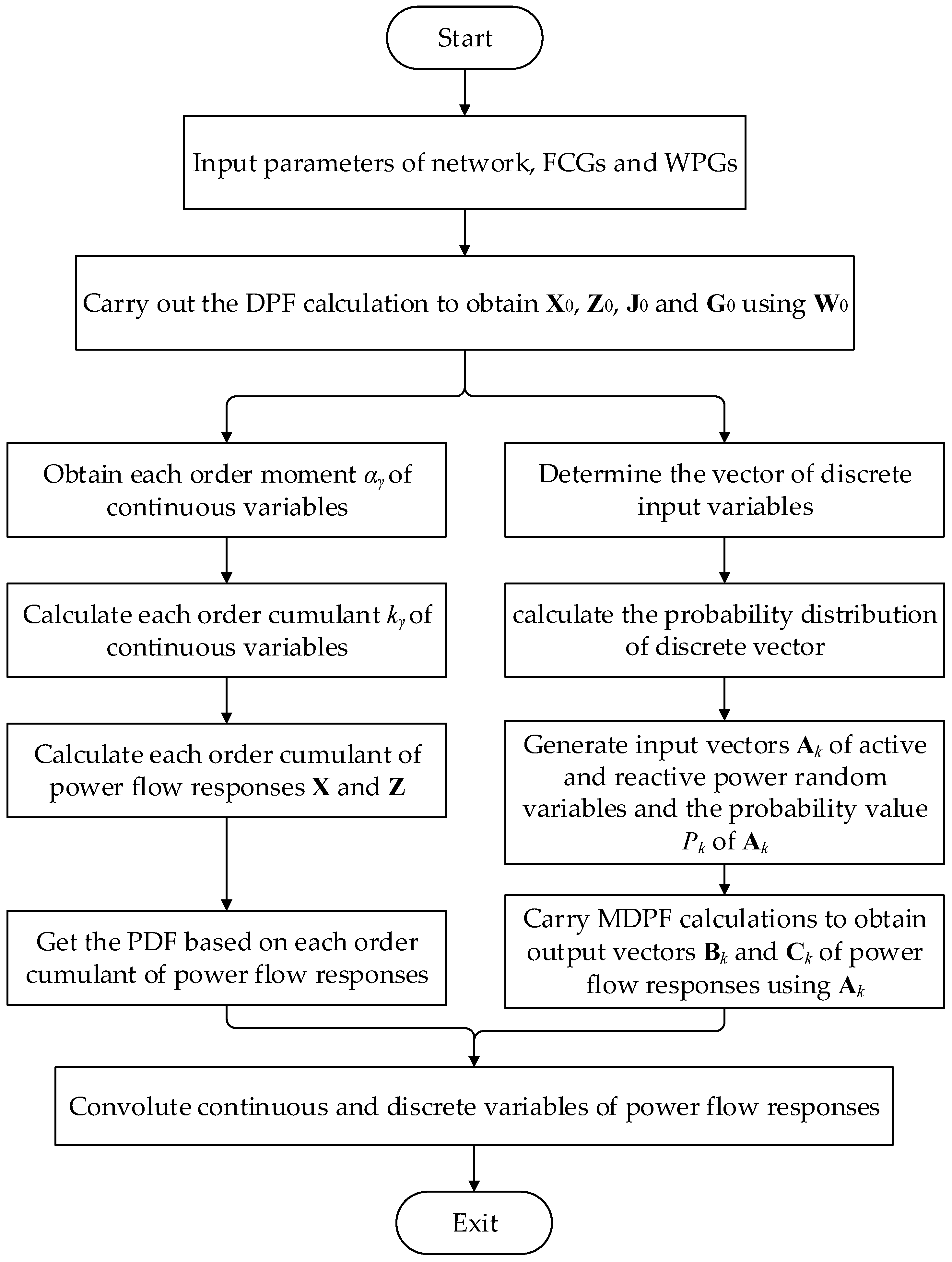
Step (10) Convolute continuous and discrete variables of power flow responses obtained, respectively, from Step 6 and Step 9 according to Equations (22) and (23). Convolution results are power flow responses considering all continuous and discrete variables. Figure 1 is the flowchart of the power flow considering continuous and discrete variables (CDPF) method.
4. Case Studies
The accuracy, efficiency, and applicability of CDPF are verified in this section, including four parts: (1) The CDPF, MCSM, and CM are used to solve PPF problems in an IEEE 14-bus power system. Compared with CM, CDPF has better accuracy; and compared with MCSM, CDPF has higher efficiency; (2) PPF problems on a FCG under different rated powers are studied to further demonstrate the applicability of CDPF in an IEEE 14-bus power system; (3) the case of multiple FCGs in a power system is considered to demonstrate the applicability of CDPF in an IEEE 14-bus power system; and (4) an IEEE bus-118 power system is applied to verify the performance of CDPF.
4.1. Verification of CDPF by Comparison with MCSM and CM in Accuracy and Efficiency
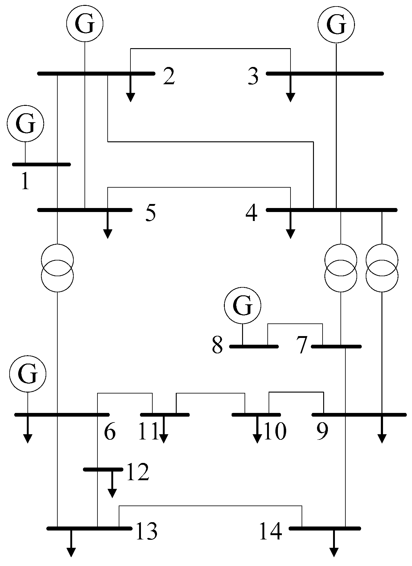
An IEEE 14-bus power system is used in this part, consisting of 14 buses and 20 branches. Figure 2 is the IEEE 14-bus power system. The loads are supposed to follow a normal distribution, in which mean values are the power value of loads, and standard deviations are 5% of mean values. A WPG with a capability of 10 MW is connected to bus-13, and the constant power control method is adopted in WPG with the power factor cos(φ) = −0.98, the cut-in wind speed of WPG is vci = 3 m/s, the rated wind speed of WPG is vr = 15 m/s, and the cut-out wind speed of WPG is vco = 25 m/s. The wind speed model is assumed to follow a two-parameter Weibull distribution with a shape parameter k = 2.80 and a scale parameter c = 5.14. Two FCGs are connected to bus-13 and bus-14, where each capability of FCG is 20 MW, the power factor cos(φ) = 0.8, and the outage probability is 0.08. DPF calculation times based on MCSM are 10,000, and MCSM is taken as a comparison standard of PPF solutions in this paper.
PDFs of the voltage magnitude of bus-14 gained by the three methods, respectively, are shown in Figure 3. PDF curves of CDPF are almost the same as the ones obtained by MCMS. However, results obtained by CM have a large difference compared with results obtained by MCMS, and negative probability values occur in Figure 3 by CM.
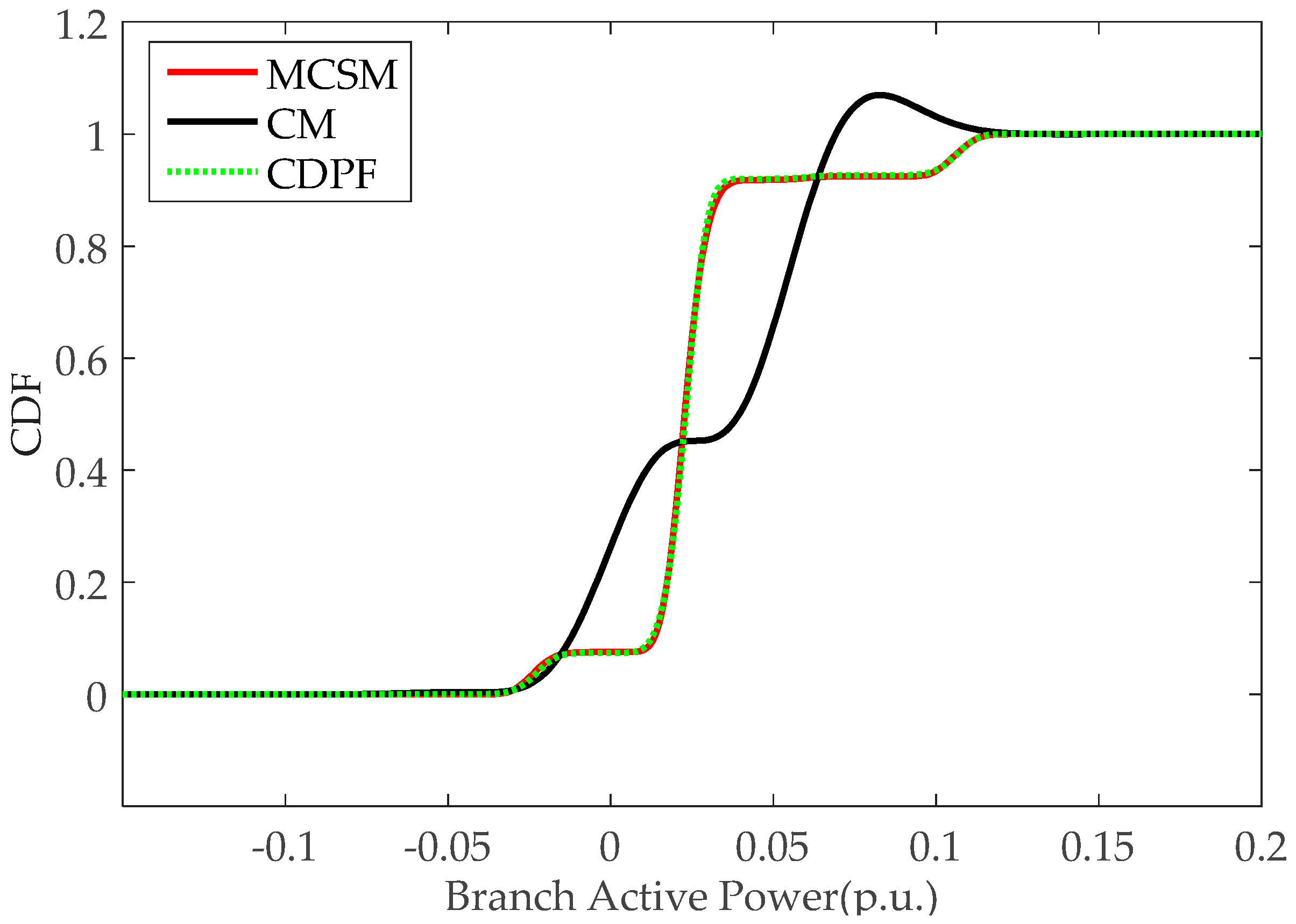
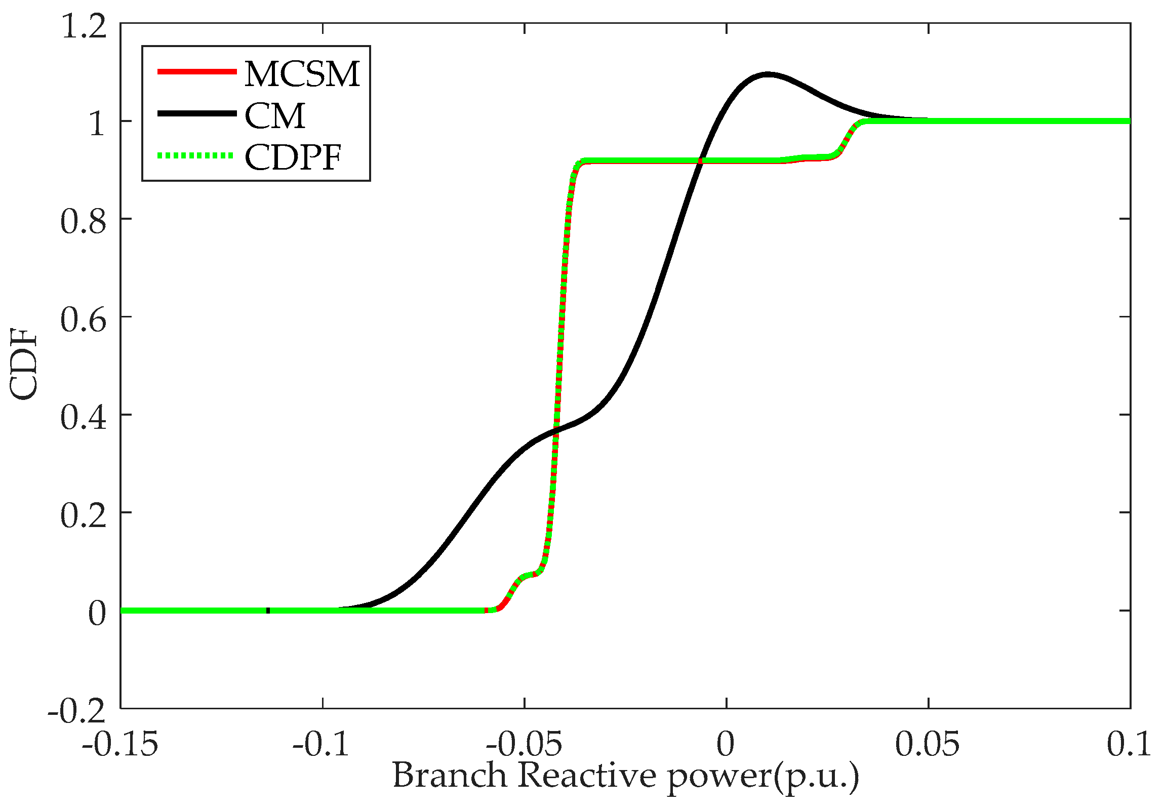
Figure 4 and Figure 5 are CDFs of the active and reactive power, respectively, at branch 20 (from bus-13 to bus-14). In Figure 4 and Figure 5, some values in the CDF curves of CM are more than 1, which violates the probability property. The reason is that the large fluctuation range of random input variables causes a large linearization error of power flow equations.
Means and standard deviations of the voltage magnitude (p.u.) and the active power (p.u.) at branches in the IEEE 14-bus power system are shown, respectively, in Table 1 and Table 2. The results obtained by CDPF are closer to standard results obtained by MCMS compared with the results obtained by CM.
The CPU time and calculation number NPL of DPF are shown in the Table 3. NPL of CDPF includes a DPF calculation based on CM to handle continuous variables and DPF calculations of 2n times to handle n discrete variables. The CPU time of CDPF also mainly includes the above two types of calculation times, in which it is the major part for handling discrete variables based on MDPF calculations. Compared with MCSM, the CPU time and NPL of CDPF can be greatly reduced. To promote calculation accuracy and reduce the CPU time and NPL, CDPF makes good use of simulation (MDPF) and analytical methods (CM). Compared with CM, the CPU time and NPL of CDPF are slightly increased because of the cost for enhancing the calculation accuracy.
4.2. PPF Analysis on a FCG under Different Rated Powers
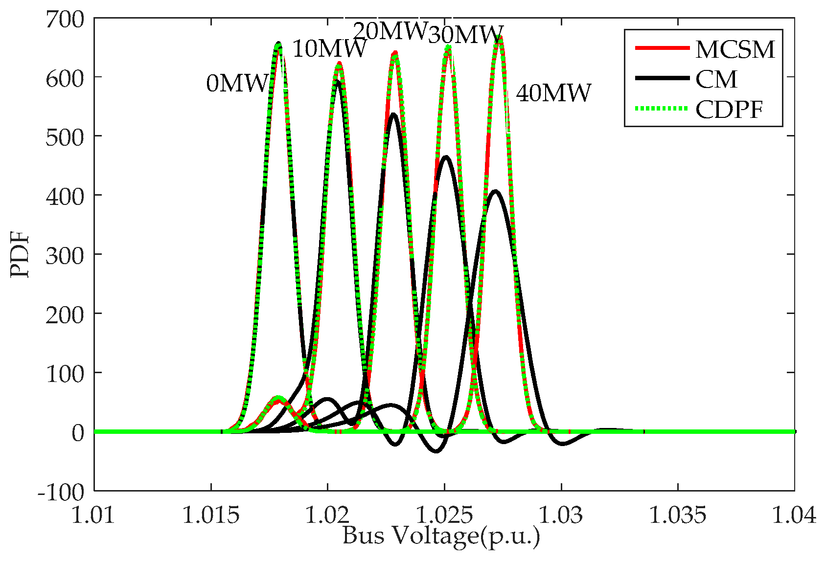
To further demonstrate the applicability of CDPF, a test of the accuracy of CDPF is carried out under an FCG with different rated powers. The FCG is only set at bus-14, and rated powers are, respectively, 0 MW, 10 MW, 20 MW, 30 MW and 40 MW. Except for the rated power of FCGs, other parameters of FCGs, positions, and parameters of WPGs are the same as those in Part 1 of Section 4.
The PDFs of the voltage magnitude at bus-14 with the rated power of the FCGs at bus-14 being 0 MW, 10 MW, 20 MW, 30 MW and 40 MW, respectively, are shown in Figure 6 by three methods. The results of CDPF are almost the same as the results of MCSM at different rated powers of the FCGs. Compared with MCSM, the accuracy of CM gradually decreases with the rated power of the FCGs gradually increasing. With the rated power of FCGs increasing, the rate of total active power of FCGs is increased, which increases the fluctuation range of discrete variables. Meanwhile, the linearization errors and the series expansion errors are both increased. Hence, the accuracy of CM decreases and the results verify this conclusion.
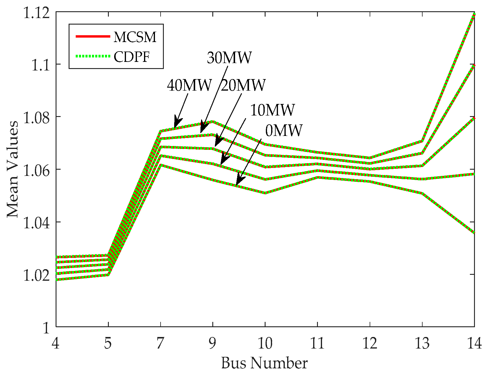
The means and standard deviations of the voltage magnitude at PQ buses with the rated power of FCG at bus-14 being 0 MW, 10 MW, 20 MW, 30 MW and 40 MW, respectively, are shown in Figure 7 and Figure 8 by MCSM and CDPF. The results of CDPF are almost the same as results of MCSM on means and standard deviations of the voltage magnitude at PQ buses.
4.3. PPF Analysis on Multiple FCGs in an IEEE 14-Bus Power System
To further demonstrate the applicability of CDPF, four cases on the accuracy and efficiency of CDPF are carried when multiple FCGs exist in an IEEE 14-bus power system. In all cases, the total power of FCGs is assumed to be constant, while the number and position of FCGs connected in the power system are alternative. In the first case, the number of FCGs connected in the IEEE 14-bus power system is one and the position of FCG is at bus-14, with the rated power of each FCG being 10 MW. In the second case, the number of FCGs connected in the IEEE 14-bus power system is two and the positions of the FCGs are at bus-13 and bus-14, with the rated power of each FCG being 5 MW. In the third case, the number of FCGs connected in the IEEE 14-bus power system is three, and positions of FCGs are at bus-12, bus-13 and bus-14, with the rated power of each FCG 3.33 MW. In the fourth case, the number of FCGs connected in the IEEE 14-bus power system is five and positions of the FCGs are at bus-10, bus-11, bus-12, bus-13 and bus-14, with the rated power of each FCG being 2 MW. Other settings of parameters, including the power system network, traditional generators, WPG, and loads, are the same as those of Part 1 in Section 4.
PDFs of the voltage magnitude at bus-14 with one, two, three, and five FCGs, respectively, at different buses in the IEEE 14-bus power system are shown in Figure 9 by three methods. The results of CDPF are almost the same as the results of MCSM in different numbers of FCGs, which is to say that solutions obtained by CDPF can match standard solutions obtained by MCSM rather well, yet the accuracy of CM gradually decreases with the number of FCGs increasing compared with MCSM. With the number of FCGs increasing, the linearization errors and the series expansion errors are both increased in CM. Hence, the accuracy of CM decreases and the results verify this conclusion.
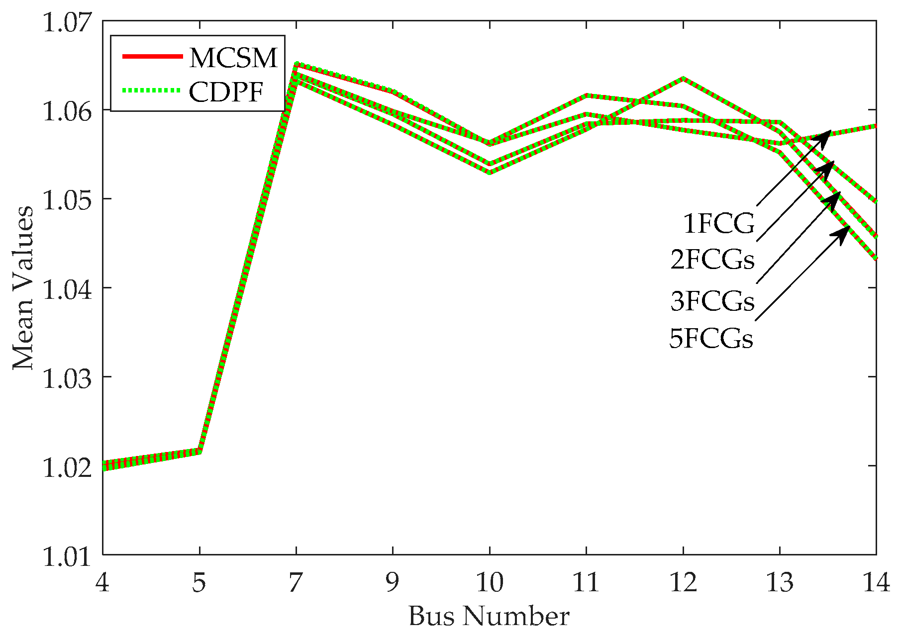
The means and standard deviations of the voltage magnitude at PQ buses with one, two, three, and five FCGs, respectively, at different buses in the IEEE 14-bus power system are shown in Figure 10 and Figure 11 by MCSM and CDPF. Results obtained by CDPF are almost the same as those obtained by MCSM with respect to means and standard deviations of the bus voltage magnitude at PQ buses.
CPU time and calculation number NPL of three methods are shown in Table 4. Compared with MCSM, CDPF requires less CPU time and NPL for each case. Note that with the number of FCGs increasing, CPU time and NPL are also increased in CDPF because computation iterations for MDPF are related to the number of FCGs.
4.4. The Test in the IEEE 118-Bus Power System
To demonstrate the applicability of CDPF on large power systems, an IEEE 118-bus power system is used in this part. Details on the IEEE 118-bus power system are: 118 buses; 186 branches; a 500 MW WPG plant is set at bus-2 and nine FCG plants are set, respectively, at bus-3, bus-5, bus-7, bus-9, bus-11, bus-13, bus-14, bus-16 and bus-17, the rated power of each FCG plant is 200 MW; other settings of WPGs and loads can be referred to those of Part 1 in Section 4. In the IEEE 118-bus power system, 119 continuous input variables (a WPG and 118 loads) and nine discrete input variables (nine FCGs) are considered in this paper.
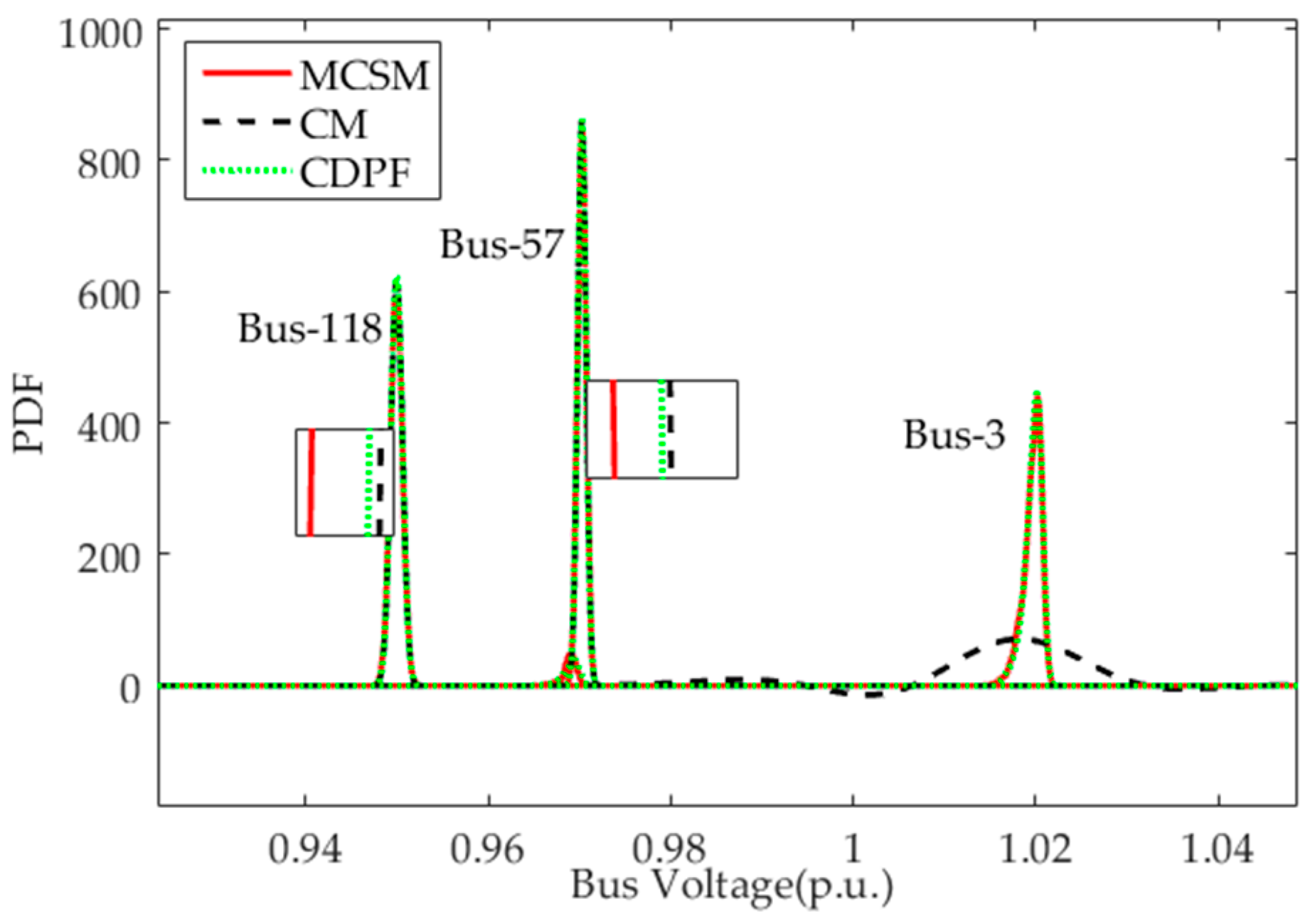
PDFs of the voltage magnitude at bus-3, bus-57 and bus-118 are shown in Figure 12 by three methods. CDPF and CM perform well with respect to the accuracy of voltage magnitudes at bus-57 and bus-118. Specifically, we can see that PDFs of the voltage magnitude at bus-57 and bus-118 obtained by CDPF are closer to that obtained by MCSM than that by CM. Especially, the accuracy of the voltage magnitude at bus-3 in CDPF is much higher than that in CM. The main reason is that bus-3 is close to WPG, and the FCGs result in a larger impact on bus-3 than on bus-57 and bus-118.
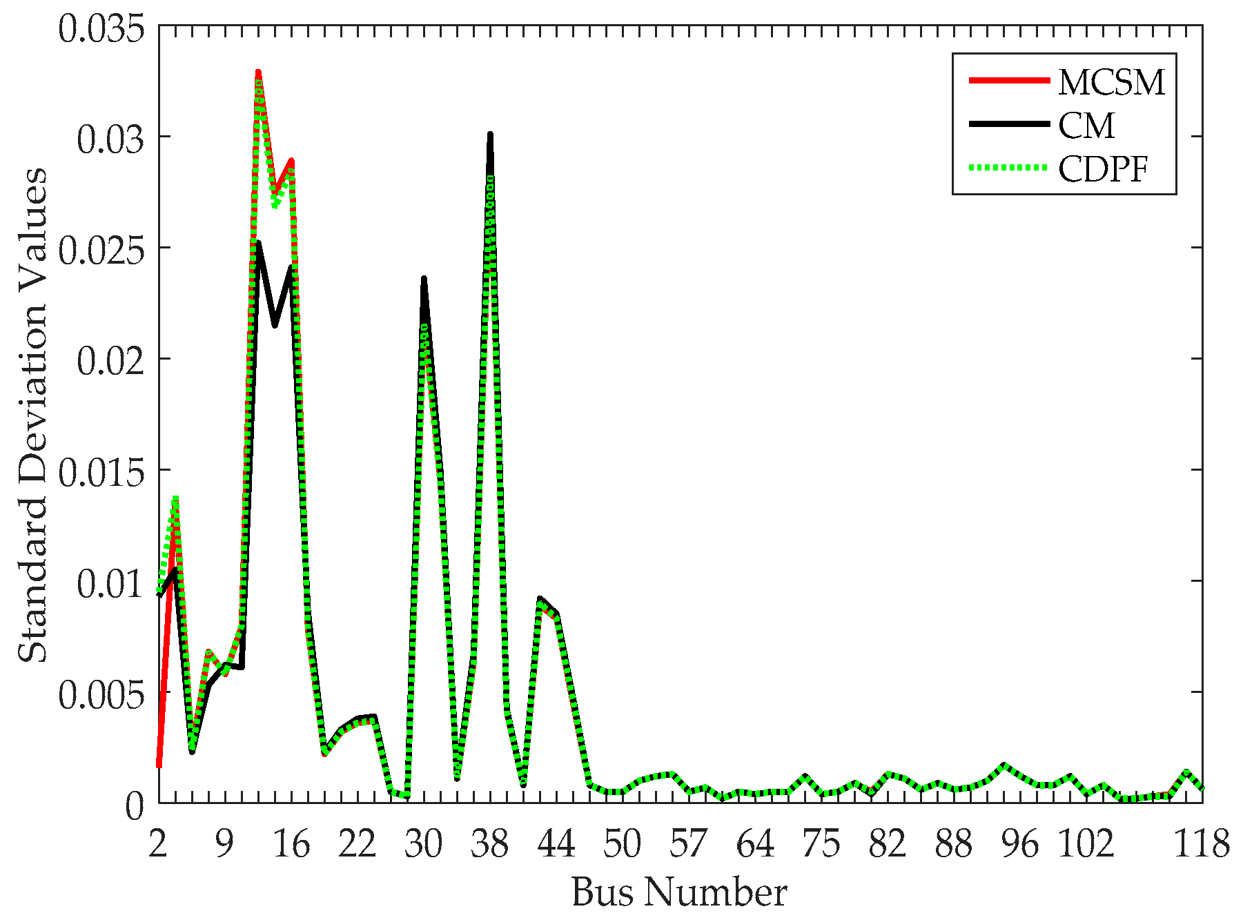
Means and standard deviations of the voltage magnitude at PQ buses in IEEE 118-bus power system are shown in Figure 13 and Figure 14. In general, CDPF and CM can well approach the standard results based on MCSM with respect to mean and standard deviation indices. Specifically, we can see that the green line denoting the CDPF is closer to the red line denoting the MCSM than the black line denoting the CM in Figure 13 and Figure 14. Yet, the standard deviation in the CM has larger errors compared with that in MCSM at some buses in Figure 14.
CPU time and calculation number NPL of three methods are shown in Table 5. CPU time and NPL of CDPF are obviously decreased compared with those in MCSM. Although CDPF’s CPU time is slightly increased compared with that in CM, CDPF can still inherit MCSM’s computational accuracy advantage and CM’s computational speed merit.
5. Conclusions
A novel PPF method considering continuous and discrete variables, called CDPF, is proposed in this paper. The mean, standard deviation, PDF, and CDF of power flow responses can be calculated accurately and efficiently by the proposed method. Continuous variables following a normal distribution or non-normal distribution and discrete variables following binomial distribution can be solved by the proposed method. The accuracy, efficiency, and applicability of the proposed method are demonstrated by comparing MCSM, CM and CDPF in IEEE 14-bus and IEEE 118-bus power systems. Conclusions are summarized as follows:
- (1)
- CDPF has better performance in computation speed compared with MCSM. Additionally, CDPF has a better performance in computation accuracy than CM, especially for the case with the large fluctuation range of input random variables.
- (2)
- CDPF has good performance in the applicability to deal with a discrete variable with different rated powers and multiple discrete variables in power systems.
- (3)
- CDPF has good performance in the applicability to address large power systems with high accuracy and efficiency.
In the future, the idea of the proposed method can be applied to other uncertainty analytical problems, such as the probabilistic static stability and the probabilistic reactive power control, and so on.
Author Contributions
Xuexia Zhang, Zhiqi Guo and Weirong Chen conceived this paper. Xuexia Zhang and Zhiqi Guo designed the experiments and analyzed the data. All authors wrote, reviewed and approved the manuscript.
Conflicts of Interest
The authors declare no conflict of interest.
Glossary of Acronyms
| PPF | probabilistic power flow |
| CM | cumulant method |
| MCSM | Monte Carlo simulation method |
| CDPF | power flow considering continuous and discrete variables |
| DPF | deterministic power flow |
| MDPF | multiple deterministic power flow |
| probability density function | |
| CDF | cumulative density function |
| GCS | Gram-Charlier series |
| FCG | fuel cell generation |
| WPG | wind power generation |
| CPU | central processing unit |
References
- Borkowska, B. Probabilistic load flow. IEEE Trans. Power Appar. Syst. 1974, 3, 752–759. [Google Scholar] [CrossRef]
- Sun, Y.Y.; Mao, R.; Li, Z.Y.; Tian, W. Constant Jacobian matrix-based stochastic Galerkin method for probabilistic load flow. Energies 2016, 9, 153. [Google Scholar] [CrossRef]
- Chen, Y.; Wen, J.Y.; Cheng, S.J. Probabilistic load flow method based on Nataf transformation and Latin hypercube sampling. IEEE Trans. Sustain. Energy 2013, 4, 294–301. [Google Scholar] [CrossRef]
- Soleimanpour, N.; Mohammadi, M. Probabilistic load flow by using nonparametric density estimators. IEEE Trans. Power Syst. 2013, 28, 3747–3755. [Google Scholar] [CrossRef]
- Zhang, S.X.; Cheng, H.Z.; Zhang, L.B.; Bazargan, M.; Yao, L.Z. Probabilistic evaluation of available load supply capability for distribution system. IEEE Trans. Power Syst. 2013, 28, 3215–3225. [Google Scholar] [CrossRef]
- Zhang, H.; Li, P. Probabilistic analysis for optimal power flow under uncertainty. IET Gener. Transm. Distrib. 2010, 4, 553–561. [Google Scholar] [CrossRef]
- Zou, B.; Xiao, Q. Solving Probabilistic optimal power flow problem using quasi Monte Carlo method and ninth-order polynomial normal transformation. IEEE Trans. Power Syst. 2014, 29, 300–306. [Google Scholar] [CrossRef]
- Kaffashan, I.; Amraee, T. Probabilistic undervoltage load shedding using point estimate method. IET Gener. Transm. Distrib. 2015, 9, 2234–2244. [Google Scholar] [CrossRef]
- Li, Y.M.; Li, W.Y.; Yan, W.; Yu, J.; Zhao, X. Probabilistic optimal power flow considering correlations of wind speeds following different distributions. IEEE Trans. Power Syst. 2014, 29, 1847–1854. [Google Scholar] [CrossRef]
- Hong, Y.Y.; Lin, F.J.; Yu, T.H. Taguchi method-based probabilistic load flow studies considering uncertain renewables and loads. IET Renew. Power Gener. 2016, 10, 221–227. [Google Scholar] [CrossRef]
- Rouhani, M.; Mohammadi, M.; Kargarian, A. Parzen window density estimator-based probabilistic power flow with correlated uncertainties. IEEE Trans. Sustain. Energy 2016, 7, 1170–1181. [Google Scholar] [CrossRef]
- Villanueva, D.; Feijόo, A.E.; Pazos, J.L. An analytical method to solve the probabilistic load flow considering load demand correlation using the DC load flow. Electr. Power Syst. Res. 2014, 110, 1–8. [Google Scholar] [CrossRef]
- Mohammadi, M. Probabilistic harmonic load flow using fast point estimate method. IET Gener. Transm. Distrib. 2015, 9, 1790–1799. [Google Scholar] [CrossRef]
- Ren, Z.Y.; Li, W.Y.; Billinton, R.; Yan, W. Probabilistic power flow analysis based on the stochastic response surface method. IEEE Trans. Power Syst. 2016, 31, 2307–2315. [Google Scholar] [CrossRef]
- Ruiz-Rodriguez, F.J.; Hernández, J.C.; Jurado, F. Probabilistic load flow for photovoltaic distributed generation using the cornish-fisher expansion. Electr. Power Syst. Res. 2012, 89, 129–138. [Google Scholar] [CrossRef]
- Tamtum, A.; Schellenberg, A.; Rosehart, W.D. Enhancements to the cumulant method for probabilistic optimal power flow studies. IEEE Trans. Power Syst. 2009, 24, 1739–1746. [Google Scholar] [CrossRef]
- Hajian, M.; Rosehart, W.D.; Zareipour, H. Probabilistic power flow by Monte Carlo simulation with Latin supercube sampling. IEEE Trans. Power Syst. 2013, 28, 1550–1559. [Google Scholar] [CrossRef]
- Long, C.; Farrag, M.E.A.; Hepburn, D.M.; Zhou, C.K. Point estimate method for voltage unbalance evaluation in residential distribution networks with high penetration of small wind turbines. Energies 2014, 7, 7717–7731. [Google Scholar] [CrossRef]
- Zhang, P.; Lee, S.T. Probabilistic load flow computation using the method of combined cumulants and Gram-Charlier expansion. IEEE Trans. Power Syst. 2004, 19, 676–682. [Google Scholar] [CrossRef]
- Liu, J.; Hao, X.D.; Cheng, P.F.; Fang, W.L.; Niu, S.B. A parallel probabilistic load flow method considering nodal correlations. Energies 2016, 9, 1041. [Google Scholar] [CrossRef]
- Bu, S.Q.; Du, W.; Wang, H.F.; Chen, Z.; Xiao, L.Y.; Li, H.F. Probabilistic analysis of small-signal stability of large-scale power systems as affected by penetration of wind generation. IEEE Trans. Power Syst. 2012, 27, 762–770. [Google Scholar] [CrossRef]
- Fan, M.; Vittal, V.; Heydt, G.T.; Ayyanar, R. Probabilistic power flow analysis with generation dispatch including photovoltaic resources. IEEE Trans. Power Syst. 2013, 28, 1797–1805. [Google Scholar] [CrossRef]
- Hong, Y.Y.; Lin, F.J.; Lin, Y.C.; Hsu, F.Y. Chaotic PSO-based VAR considering renewables using fast probabilistic power flow. IEEE Trans. Power Deliv. 2014, 29, 1666–1674. [Google Scholar] [CrossRef]
- Sanabria, L.A.; Dillon, T.S. Stochastic power flow using cumulants and Von Mises functions. Int. J. Electr. Power Energy Syst. 1986, 8, 47–60. [Google Scholar] [CrossRef]
- Hu, Z.C.; Wang, X.F. A probabilistic load flow method considering branch outages. IEEE Trans. Power Syst. 2006, 21, 507–514. [Google Scholar] [CrossRef]
- Leite da Silva, A.M.; Arienti, V.L. Probabilistic load flow by a multilinear simulation algorithm. Proc. Inst. Electr. Eng. C Gener. Transm. Distrib. 1990, 137, 276–282. [Google Scholar] [CrossRef]
- Li, Y.C.; Sun, G.Q.; Qian, X.R.; Shen, H.P.; Wei, Z.N.; Sun, Y.H. Probabilistic power flow calculation method of power system considering input variables with discrete distribution. Power Syst. Technol. 2015, 39, 3254–3259. [Google Scholar]
- Wu, W.; Wang, K.Y.; Li, G.J.; Jiang, X.C.; Wang, Z.M. Probabilistic load flow calculation using cumulants and multiple integrals. IET Gener. Transm. Distrib. 2016, 10, 1703–1709. [Google Scholar] [CrossRef]
- Cai, D.F.; Chen, J.F.; Shi, D.Y.; Duan, X.Z.; Li, H.J.; Yao, M.Q. Enhancements to the cumulant method for probabilistic load flow studies. In Proceedings of the 2012 IEEE Power and Energy Society General Meeting, San Diego, CA, USA, 22–26 July 2012. [Google Scholar]
- Morales, J.M.; Perez-Ruiz, J. Point estimate schemes to solve the probabilistic power flow. IEEE Trans. Power Syst. 2007, 22, 1594–1601. [Google Scholar] [CrossRef]
- Capitanescu, F.; Wehenkel, L. Sensitivity-based approaches for handling discrete variables in optimal power flow computations. IEEE Trans. Power Syst. 2010, 25, 1780–1789. [Google Scholar] [CrossRef]
- Niknam, T.; Bornapour, M.; Gheisari, A. Combined heat, power and hydrogen production optimal planning of fuel cell power plants in distribution networks. Energy Convers. Manag. 2013, 66, 11–25. [Google Scholar] [CrossRef]
- Fan, M.; Vittal, V.; Heydt, G.T.; Ayyanar, R. Probabilistic power flow studies for transmission systems with photovoltaic generation using cumulants. IEEE Trans. Power Syst. 2012, 27, 2251–2261. [Google Scholar] [CrossRef]
- Ruiz-Rodriguez, F.J.; Hernandez, J.C.; Jurado, F. Probabilistic load flow for radial distribution networks with photovoltaic generators. IET Renew. Power Gener. 2012, 6, 110–121. [Google Scholar] [CrossRef]
- Williams, T.; Crawford, C. Probabilistic load flow modeling comparing maximum entropy and Gram-Charlier probability density function reconstructions. IEEE Trans. Power Syst. 2013, 28, 272–280. [Google Scholar] [CrossRef]
Figure 1.
Flowchart of the power flow considering continuous and discrete variables (CDPF) method. DPF: deterministic power flow; FCG: fuel cell generator; PDF: probability density function; MDPF: multiple DPF; WPG: wind power generator.
Figure 1.
Flowchart of the power flow considering continuous and discrete variables (CDPF) method. DPF: deterministic power flow; FCG: fuel cell generator; PDF: probability density function; MDPF: multiple DPF; WPG: wind power generator.

Figure 2.
IEEE 14-bus power system.

Figure 3.
The probability density function (PDF) of the voltage magnitude at bus-14 in an IEEE 14-bus power system. CM: cumulant method; MCSM: Monte Carlo simulation method.
Figure 3.
The probability density function (PDF) of the voltage magnitude at bus-14 in an IEEE 14-bus power system. CM: cumulant method; MCSM: Monte Carlo simulation method.
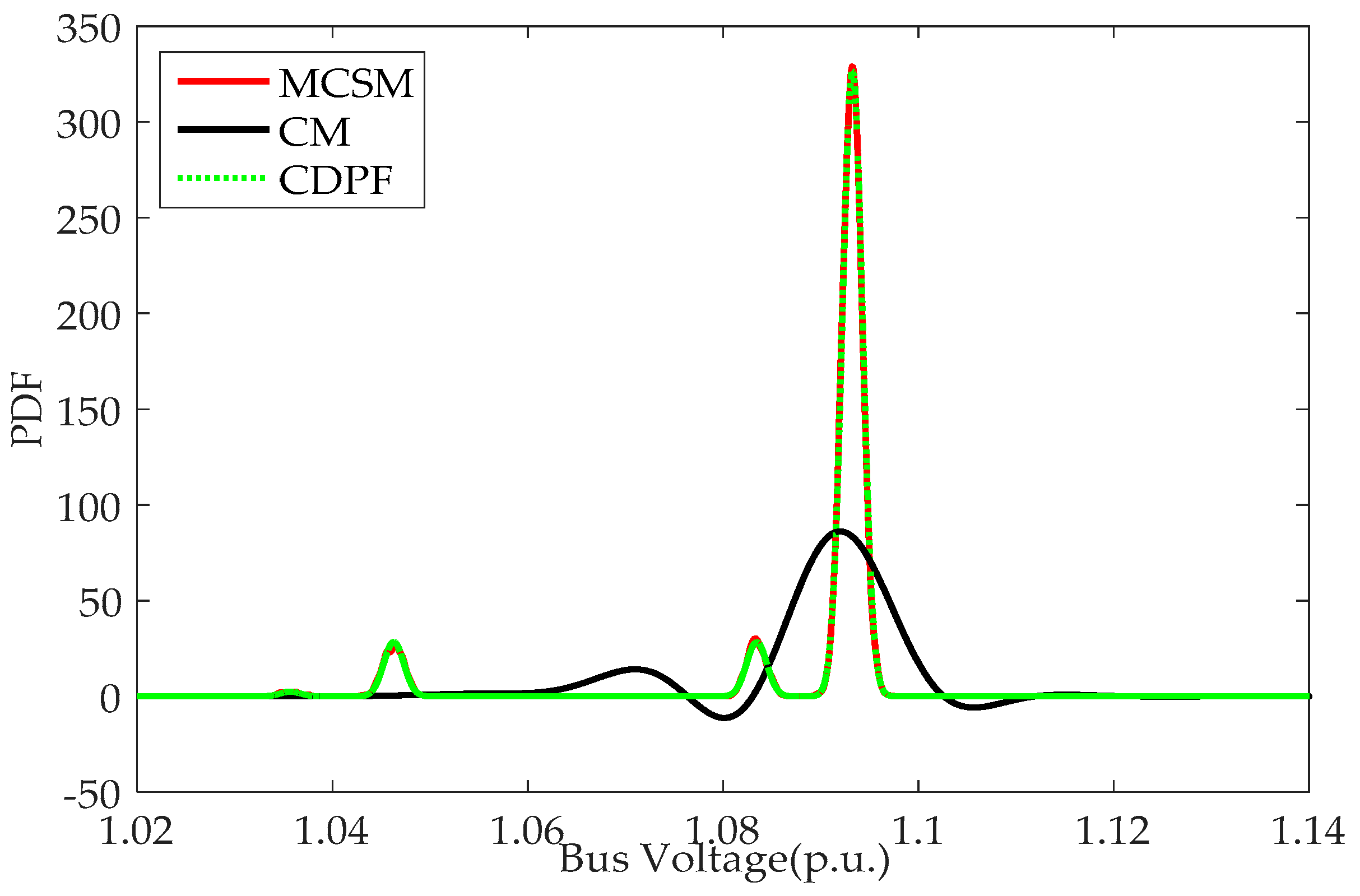
Figure 4.
The cumulative density function (CDF) of the active power at branch 20 (13–14) in an IEEE 14-bus power system.
Figure 4.
The cumulative density function (CDF) of the active power at branch 20 (13–14) in an IEEE 14-bus power system.

Figure 5.
The CDF of the reactive power at branch 20 (13–14) in an IEEE 14-bus power system.

Figure 6.
The PDFs of the voltage magnitude at bus-14 with the rated power of FCG at bus-14 being 0 MW, 10 MW, 20 MW, 30 MW and 40 MW, respectively, in an IEEE 14-bus power system.
Figure 6.
The PDFs of the voltage magnitude at bus-14 with the rated power of FCG at bus-14 being 0 MW, 10 MW, 20 MW, 30 MW and 40 MW, respectively, in an IEEE 14-bus power system.

Figure 7.
The means of the voltage magnitude at PQ buses with the rated power of the FCG at bus-14 being 0 MW, 10 MW, 20 MW, 30 MW and 40 MW, respectively, in an IEEE 14-bus power system.
Figure 7.
The means of the voltage magnitude at PQ buses with the rated power of the FCG at bus-14 being 0 MW, 10 MW, 20 MW, 30 MW and 40 MW, respectively, in an IEEE 14-bus power system.

Figure 8.
The standard deviations of the voltage magnitude at PQ buses with the rated power of the FCG at bus-14 being 0 MW, 10 MW, 20 MW, 30 MW and 40 MW, respectively, in an IEEE 14-bus power system.
Figure 8.
The standard deviations of the voltage magnitude at PQ buses with the rated power of the FCG at bus-14 being 0 MW, 10 MW, 20 MW, 30 MW and 40 MW, respectively, in an IEEE 14-bus power system.
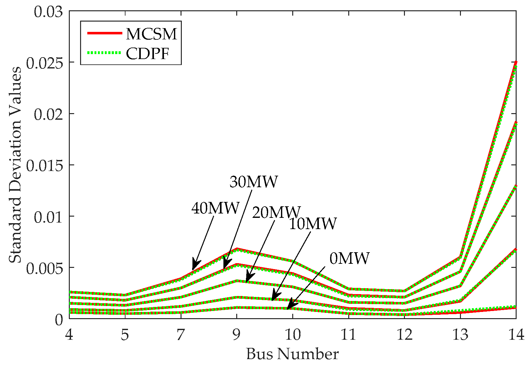
Figure 9.
The PDFs of the voltage magnitude at bus-14 with one, two, three and five FCGs, respectively, at different buses in an IEEE 14-bus power system.
Figure 9.
The PDFs of the voltage magnitude at bus-14 with one, two, three and five FCGs, respectively, at different buses in an IEEE 14-bus power system.
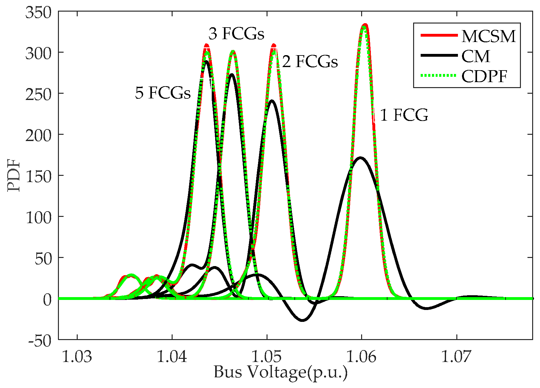
Figure 10.
The means of the voltage magnitude at PQ buses with one, two, three and five FCGs, respectively, at different buses in an IEEE 14-bus power system.
Figure 10.
The means of the voltage magnitude at PQ buses with one, two, three and five FCGs, respectively, at different buses in an IEEE 14-bus power system.

Figure 11.
Standard deviations of the voltage magnitude at PQ buses with one, two, three and five FCGs, respectively, at different buses in an IEEE 14-bus power system.
Figure 11.
Standard deviations of the voltage magnitude at PQ buses with one, two, three and five FCGs, respectively, at different buses in an IEEE 14-bus power system.
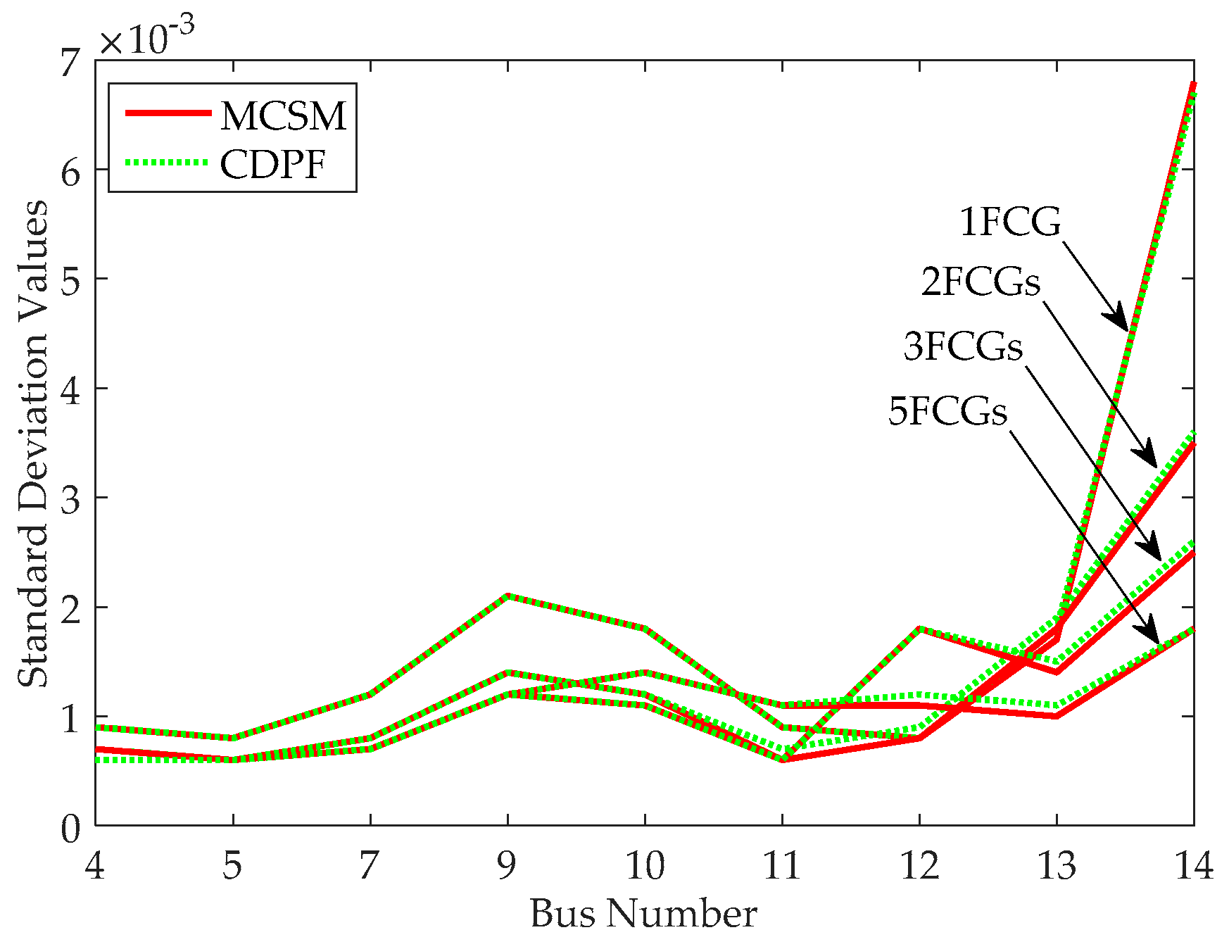
Figure 12.
The PDFs of the voltage magnitude at bus-3, bus-57 and bus-118 in an IEEE 118-bus power system.
Figure 12.
The PDFs of the voltage magnitude at bus-3, bus-57 and bus-118 in an IEEE 118-bus power system.

Figure 13.
The means of the voltage magnitude at PQ buses in an IEEE 118-bus power system.
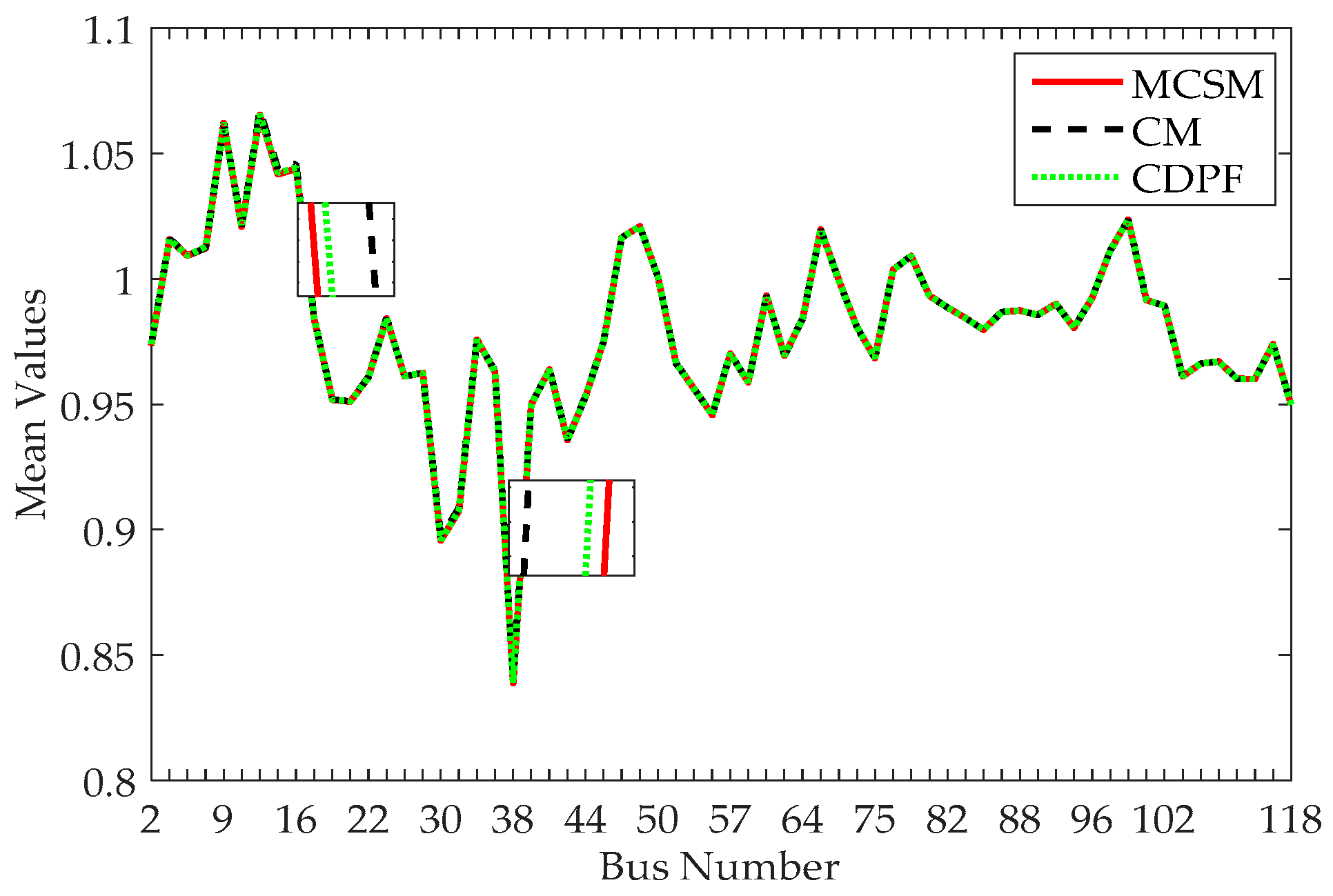
Figure 14.
The Standard deviations of the bus voltage magnitude at PQ buses in an IEEE 118-bus power system.
Figure 14.
The Standard deviations of the bus voltage magnitude at PQ buses in an IEEE 118-bus power system.


Table 1.
The means and standard deviations of the voltage magnitude (p.u.) in an IEEE 14-bus power system.
Table 1.
The means and standard deviations of the voltage magnitude (p.u.) in an IEEE 14-bus power system.
| Bus No. | Mean Values | Standard Deviation Values | ||||
|---|---|---|---|---|---|---|
| MCSM | CM | CDPF | MCSM | CM | CDPF | |
| 1 | 1.0600 | 1.0600 | 1.0600 | 0.0000 | 0.0000 | 0.0000 |
| 2 | 1.0450 | 1.0450 | 1.0450 | 0.0000 | 0.0000 | 0.0000 |
| 3 | 1.0100 | 1.0100 | 1.0100 | 0.0000 | 0.0000 | 0.0000 |
| 4 | 1.0250 | 1.0251 | 1.0250 | 0.0016 | 0.0012 | 0.0016 |
| 5 | 1.0266 | 1.0267 | 1.0266 | 0.0015 | 0.0012 | 0.0015 |
| 6 | 1.0700 | 1.0700 | 1.0700 | 0.0000 | 0.0000 | 0.0000 |
| 7 | 1.0699 | 1.0700 | 1.0699 | 0.0021 | 0.0016 | 0.0021 |
| 8 | 1.0900 | 1.0900 | 1.0900 | 0.0000 | 0.0000 | 0.0000 |
| 9 | 1.0693 | 1.0624 | 1.0693 | 0.0036 | 0.0030 | 0.0036 |
| 10 | 1.0619 | 1.0620 | 1.0619 | 0.0030 | 0.0025 | 0.0030 |
| 11 | 1.0624 | 1.0624 | 1.0624 | 0.0016 | 0.0013 | 0.0016 |
| 12 | 1.0690 | 1.0690 | 1.0690 | 0.0030 | 0.0028 | 0.0030 |
| 13 | 1.0808 | 1.0809 | 1.0809 | 0.0066 | 0.0055 | 0.0065 |
| 14 | 1.0886 | 1.0889 | 1.0887 | 0.0131 | 0.0094 | 0.0131 |
Table 2.
The means and standard deviations of the active power (p.u.) at the branches in an IEEE 14-bus power system.
Table 2.
The means and standard deviations of the active power (p.u.) at the branches in an IEEE 14-bus power system.
| Bus No. | Mean Values | Standard Deviation Values | ||||
|---|---|---|---|---|---|---|
| MCSM | CM | CDPF | MCSM | CM | CDPF | |
| 1 | 1.2985 | 1.2982 | 1.2987 | 0.0709 | 0.0708 | 0.0712 |
| 2 | 0.6044 | 0.6043 | 0.6046 | 0.0349 | 0.0350 | 0.0352 |
| 3 | 0.6790 | 0.6790 | 0.6791 | 0.0299 | 0.0299 | 0.0300 |
| 4 | 0.4572 | 0.4571 | 0.4572 | 0.0239 | 0.0242 | 0.0241 |
| 5 | 0.3160 | 0.3159 | 0.3161 | 0.0211 | 0.0211 | 0.0213 |
| 6 | 0.2829 | 0.2831 | 0.2830 | 0.0238 | 0.0238 | 0.0239 |
| 7 | 0.5917 | 0.5917 | 0.5917 | 0.0204 | 0.0211 | 0.0205 |
| 8 | 0.1723 | 0.1723 | 0.1724 | 0.0235 | 0.0246 | 0.0237 |
| 9 | 0.0990 | 0.0990 | 0.0991 | 0.0134 | 0.0141 | 0.0135 |
| 10 | 0.2250 | 0.2249 | 0.2253 | 0.0441 | 0.0430 | 0.0446 |
| 11 | 0.0902 | 0.0902 | 0.0902 | 0.0088 | 0.0089 | 0.0090 |
| 12 | 0.0251 | 0.0251 | 0.0252 | 0.0111 | 0.0101 | 0.0113 |
| 13 | 0.0023 | 0.0024 | 0.0021 | 0.0375 | 0.0391 | 0.0380 |
| 14 | 0.0000 | 0.0000 | 0.0000 | 0.0000 | 0.0000 | 0.0000 |
| 15 | 0.1723 | 0.1723 | 0.1724 | 0.0235 | 0.0246 | 0.0237 |
| 16 | 0.0359 | 0.0359 | 0.0360 | 0.0092 | 0.0091 | 0.0093 |
| 17 | 0.0596 | 0.0597 | 0.0595 | 0.0345 | 0.0359 | 0.0348 |
| 18 | 0.0543 | 0.0543 | 0.0543 | 0.0087 | 0.0086 | 0.0088 |
| 19 | 0.0360 | 0.0360 | 0.0359 | 0.0110 | 0.0103 | 0.0112 |
| 20 | 0.0258 | 0.0256 | 0.0258 | 0.0261 | 0.0261 | 0.0263 |
Table 3.
CPU time and calculation number NPL of the DPF.
| MCSM | CM | CDPF | |||
|---|---|---|---|---|---|
| NPL | CPU Time (s) | NPL | CPU Time (s) | NPL | CPU Time (s) |
| 10,000 | 181.0645 | 1 | 0.0800 | 5 | 0.3144 |
Notes: NPL is the calculation number of the DPF; CPU: Central Processing Unit.
Table 4.
CPU time and calculation number NPL of DPF.
| FCG Number | MCSM | CM | CDPF | |||
|---|---|---|---|---|---|---|
| NPL | CPU Time (s) | NPL | CPU Time (s) | NPL | CPU Time (s) | |
| 1 | 10,000 | 183.3972 | 1 | 0.0623 | 3 | 0.1461 |
| 2 | 10,000 | 180.8913 | 1 | 0.0624 | 5 | 0.2492 |
| 3 | 10,000 | 182.4137 | 1 | 0.0671 | 9 | 0.4970 |
| 5 | 10,000 | 183.9572 | 1 | 0.0661 | 33 | 2.0045 |
Table 5.
CPU time and calculation number NPL of DPF.
| MCSM | CM | CDPF | |||
|---|---|---|---|---|---|
| NPL | CPU Time (s) | NPL | CPU Time (s) | NPL | CPU Time (s) |
| 10,000 | 526.2479 | 1 | 0.2052 | 513 | 71.2006 |
© 2017 by the authors. Licensee MDPI, Basel, Switzerland. This article is an open access article distributed under the terms and conditions of the Creative Commons Attribution (CC BY) license (http://creativecommons.org/licenses/by/4.0/).
Share and Cite
MDPI and ACS Style
Zhang, X.; Guo, Z.; Chen, W. Probabilistic Power Flow Method Considering Continuous and Discrete Variables. Energies 2017, 10, 590. https://doi.org/10.3390/en10050590
AMA Style
Zhang X, Guo Z, Chen W. Probabilistic Power Flow Method Considering Continuous and Discrete Variables. Energies. 2017; 10(5):590. https://doi.org/10.3390/en10050590
Chicago/Turabian StyleZhang, Xuexia, Zhiqi Guo, and Weirong Chen. 2017. "Probabilistic Power Flow Method Considering Continuous and Discrete Variables" Energies 10, no. 5: 590. https://doi.org/10.3390/en10050590
Note that from the first issue of 2016, this journal uses article numbers instead of page numbers. See further details here.