
An Investigation of the Restitution Coefficient Impact on Simulating Sand-Char Mixing in a Bubbling Fluidized Bed


School of Energy and Power Engineering, Beihang University, Beijing 100191, China
*
Author to whom correspondence should be addressed.
Energies 2017, 10(5), 617; https://doi.org/10.3390/en10050617
Submission received: 17 March 2017
/
Revised: 19 April 2017
/
Accepted: 27 April 2017
/
Published: 3 May 2017
(This article belongs to the Special Issue Engineering Fluid Dynamics)
Abstract
:In the present work, the effect of the restitution coefficient on the numerical results for a binary mixture system of sand particles and char particles in a bubbling fluidized bed with a huge difference between the particles in terms of density and volume fraction has been studied based on two-fluid model along with the kinetic theory of granular flow. Results show that the effect of restitution coefficient on the flow characteristics varies in different regions of the bed, which is more evident for the top region of the bed. The restitution coefficient can be categorized into two classes. The restitution coefficients of 0.7 and 0.8 can be included into one class, whereas the restitution coefficient of 0.9 and 0.95 can be included into another class. Moreover, four vortices can be found in the time-averaged flow pattern distribution, which is very different from the result obtained for the binary system with the similar values between particles in density and volume fraction.
1. Introduction
Bubbling fluidized beds are commonly used in industrial processes [1], such as combustion and gasification, due to their good mixing ability and heat transfer characteristic between the gas and solid phases. In the process of biomass gasification, the first step is pyrolysis. The gas component products after pyrolysis are non-condensable gases and tars, and char is left as a solid residue [2]. Due to the irregular shape and low density of char particles, it is difficult to attain a stable fluidization status. Generally, inert particles such as sand particles are added to the fluidized bed to improve the fluidization status and the heat transfer effect. During the process of fluidization, char particles will accumulate toward the top of the bed, whereas the inert particles will sink towards the bottom of the bed. Hence, segregation is a widespread phenomenon in a binary system of particles in a bubbling fluidized bed [3,4].
The complicated flow characteristics in the bubbling fluidized bed have a strong effect on the reaction process. Therefore understanding the flow behavior is important to design a fluidized bed and optimize the operation conditions. Although the most accurate method is still based on the experimental data, the application of this method has limitations, in terms of the longer time required and high costs. With advances in computational fluid dynamics (CFD), simulation studies have become a useful method to analyze the flow characteristics in bubbling fluidized beds [5,6]. The most widely used approach for simulating dense gas-solid flow is the Eulerian–Eulerian model (two fluid model) along with the kinetic theory of granular flow [7,8].
The main parameters affecting the simulation results include the drag model, particle collision characteristics, and solid phase wall boundary conditions. The particle collision characteristics are defined based on the restitution coefficient, and the wall boundary conditions are defined in at least three ways, which are the traditional no-slip boundary conditions and two partial slip conditions [9,10]. The effects of these parameters on the simulation results have been studied by some researchers. Chao et al. [10] and Bai et al. [11] focused on the effect of the drag model on the mixing and segregation behavior of biomass mixtures in a fluidized bed. Tagliaferri et al. [12] and Mostafazadeh et al. [13] have studied the influence of the restitution coefficient on the flow dynamics of a binary solid mixture. Zhong et al. [14] have investigated the influence of wall boundary conditions on the concentration and velocity distribution of particles. In these studies, the density or volume fraction of binary particles was usually similar. However, in actual biomass gasification, the char has lower density than the sand. Meanwhile, the char generated from the pyrolysis will continue to react with the gases, hence, the volume fraction of the char in the solid phase mixtures is very low [15]. When the simulation conditions do not agree with actual situation, the reasonability and accuracy of simulation results is questionable.
Many studies [16,17,18] have studied the suitability of different drag models. Generally, the Gidaspow drag model is suitable for simulation in a dense bubbling fluidized bed. Loha et al. [6] reported that the model predictions were sensitive to the specularity coefficient and the simulation results with a higher value of specularity coefficient were in good agreement with the experimental results. According to a comparison of the differences between the specularity coefficients of one wall boundary conditions and traditional no-slip wall boundary conditions, Zhong et al. [19] found that the no-slip wall boundary condition was more suitable for simulating the dynamic segregation process of binary particles. In this study, based on a Gidaspow drag model and no-slip wall boundary conditions, a simulation is carried out to investigate the effect of the restitution coefficient on the segregation and flow characteristics of a binary particles system in a bubbling fluidized bed with a huge difference between the particles in terms of density and volume fraction. The particle system consists of char particles and sand particles with bulk density of 120 and 1590 kg/m3 and volume fraction of 11% and 89%. According to the comparison of results between computation and experiment, a suitable scope of the restitution coefficient is determined, and meanwhile, the effect of different particles characteristics in the binary mixture on the fluid dynamic behavior is also compared.
2. Model Description
In the two fluid model (TFM), the gas and solid phases are considered as inter-penetrating continua, hence the governing equations for the solid phase are similar to those for the gas phase. For the case of cold fluidization with no chemical reactions, the conservation equations for mass and momentum are represented as follows:
The continuity equation for the gas phase is expressed as follows:
The continuity equation for the sth solid phase is written as:
The momentum balance equation for the gas phase is as follows:
The momentum balance equation for the sth solid phase can be written as:
The total volume fraction of the phases is equal to 1 and it is expressed in the following way:
where t is the time. The subscript “g” refers to the gas phase and the subscript “s” refers to the sth solid phase. , , and are the acceleration due to the gravity, velocity vector, and stress-strain tensor, respectively. p, α, and ρ are the pressure, volume fraction, and density, respectively. K is the momentum exchange coefficient between phases.
The solid pressure is evaluated using the expression proposed by Lun et al. [20], and it is composed of a kinetic term and a second term due to particle collisions:
where g0,ss and are the radial distribution function and granular temperature of the sth solid phase, respectively. ess is the restitution coefficient for particle collision, which quantifies the elasticity of particle collision.
3. Simulation Setup
In this study, the experimental setup by Park et al. [21] forms the basis for the simulation. The geometry of the rectangular fluidized bed with 200 mm width and 50 mm depth is schematically shown in Figure 1. In the experiments, sand particles and char particles are used. The properties of the particles in this study are summarized in Table 1.
The 2D simulation is carried out using the TFM method, and the computational domain is accordingly set to be 200 mm width and 500 mm height. The mesh geometry and coordinate system is schematically shown in Figure 2. The Z direction represents the axial direction or height direction, whereas X direction represents the radial direction or lateral direction.
In the simulation, ambient air is used as the fluidizing medium. Meanwhile, the uniform gas velocity is specified at the bottom of the bed and the atmospheric pressure boundary condition is used at outlet of the bed. The detailed parameters including the material properties and operating conditions for simulation are summarized in Table 2.
At the beginning of the computation, the sand particles and char particles are perfectly mixed at the indicated ratio. A time step of 5 × 10⁻⁴ s was employed in the simulation using Fluent 15.0 software. When TFM is used for the simulation, the grid size should be much smaller than the physical dimensions of the geometry. Meanwhile, it should also be bigger than the particle diameter, which will ensure that the solid phase can be treated as a continuous flow. Therefore, the grid size has a drastic effect on the flow behavior [22]. A coarse grid could lead to an overprediction of the solid expansion height of the bed [23]. Sande et al. [17] found that the numerical results agree well with the experimental results when the grid size is about 10 times the particle diameter and there is no improvement in capturing homogeneous expansion when the mesh is further refined. Hence, a grid size of 5 mm was chosen in this simulation.
4. Results and Discussion
4.1. Stationary Condition
In the fluidization of the binary mixture, the particles that sink at the bottom of the bed are known as jetsam, while those that accumulate at the top of the bed are known as flotsam. In this study, the sand particles are the jetsam particles, and the char particles are the flotsam particles.
For the case with ess = 0.9, the time evolution of particle volume fraction in different layers along the height direction is monitored to obtain the statistical steady-state for solution, as shown in Figure 3. As time increases, the flotsam moves upwards while the jetsam moves downwards. Hence, with increase in time, the jetsam volume fraction increases while the flotsam volume fraction decreases at the height of 0.053 m, and the jetsam volume fraction decreases while the flotsam volume fraction increases at the height of 0.153 m. At the beginning of fluidization, the volume fractions vary rapidly, whereas the values change slowly after 30 s, corresponding to complete fluidization. Hence, the time-averaged variables are computed between 30 s and 50 s. Moreover, the result shows that the simulation time corresponding to the stationary state should be increased with increase in restitution coefficient. For the cases with ess = 0.7 and 0.8, the simulation time of 50 s is long enough. However, for ess = 0.95, the simulation has not converged to a stationary state until the time exceeds 65 s. Hence, for the case with ess = 0.95, the time-averaged variables are computed between 65 s and 85 s. When the restitution coefficient increases, it means that there is lesser dissipation of kinetic energy of particle, due to a more significant elastic particle-particle collision. This may be the reason why a longer simulation time is required before the mixing pattern reaches a stationary state when the restitution coefficient increases.
4.2. Particle Velocity and Flow Pattern
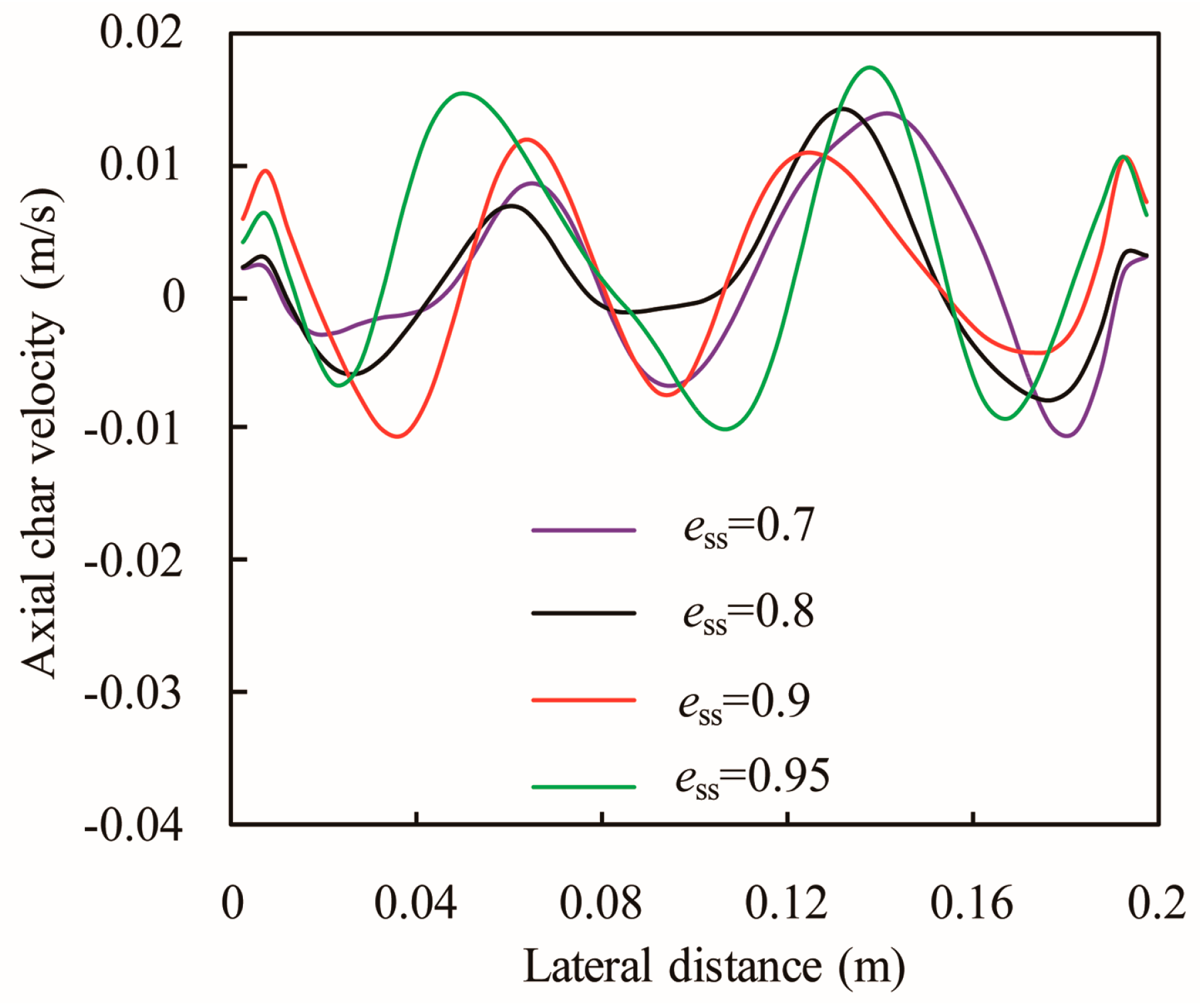
Figure 4 shows the lateral profiles of time-averaged axial velocity of the flotsam at the bed height of 0.153 m. In this figure, the velocity profiles of the flotsam for ess = 0.7, 0.8, 0.9, and 0.95 are similar. This clearly shows that the axial velocity of the flotsam is directed upward in the center of the bed and the axial velocity at the wall is nearly equal to zero, which represents the characteristic of the no-slip wall boundary condition.
In order to reflect the movement relevance between the jetsam and flotsam, in the case of ess = 0.9, the predicted flow patterns for the flotsam and jetsam are shown in Figure 5 and Figure 6, respectively. The flow patterns for the flotsam and jetsam are quite similar. Two vortices show at the bottom of the bed and two vortices close to the top of the bed. At the bottom of the bed, the particles generally rise towards the wall, whereas they fall down towards the central region. However, at the top of the bed, the movement direction of particles is reversed. The flow pattern obtained in this study is very different from the result obtained by other researchers [24]. In those studies, only two vortices can be found throughout the entire region of the dense bed layer. However, in this study, four vortices are obtained in the simulation. Moreover, the two vortices at the bottom of the bed are relatively close to the centerline of the bed, whereas the two vortices at the top of the bed are generated near the wall. It can also be seen that the distance between the two vortices at the top of the bed is farther than the value for the vortices at the bottom of the bed. This phenomenon might be due to the relationship between the binary particles in density and volume fraction. When the density and volume fraction between the binary particles changes not much [14,24], the segregation of particles does not play a leading role in fluidization process. Hence, in the top and bottom regions of the bed, uniform patterns can be found. However, in this study, a binary particles system with a huge difference between particles in density and volume fraction is used, which causes a much more notable segregation. Hence, the flow pattern of particles at the top region of the bed is different from the result for the bottom region.
The small bubbles are generally generated near the wall and the larger bubbles form near the centerline region of the bed as small bubbles move upwards [25]. Based on the analysis of positive axial velocity of particles, from Figure 5 and Figure 6, it clearly shows that the motion of particles obtained in the simulation has the same characteristics.
Due to the similar flow patterns for the flotsam and jetsam, as shown in Figure 5 and Figure 6, in the cases with same restitution coefficient, the lateral profile of the time-averaged axial velocity of the jetsam at Z = 0.153 m is similar to the profile for the flotsam. Some studies [26] have shown that the central region of the profile for jetsam changed more gently and the minimum value appeared near the wall when the layer height was at the top of the bed, which was above the jetsam-rich layer. The shape of the profile mentioned in these studies is similar with the shape of the curve obtained in the case of ess = 0.95 in this study, as shown in Figure 4.
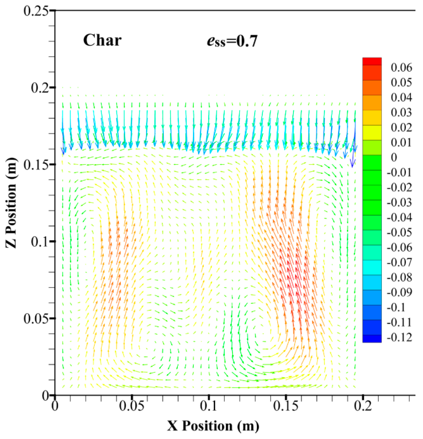
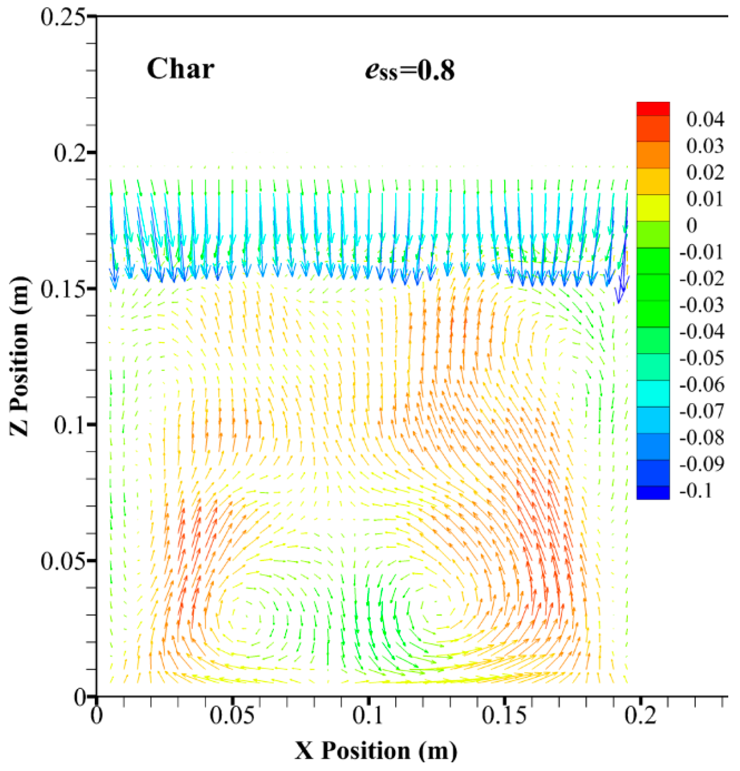
In the cases of ess = 0.7, 0.8, and 0.95, the flow patterns of the flotsam are shown in Figure 7, Figure 8 and Figure 9, respectively. The vortex structures for different restitution coefficients are similar. However, due to the lesser dissipation of granular energy, with the increase in restitution coefficient, the vortex intensity increases. At the bottom of the bed, due to the effect of the inlet gas, the restitution coefficient does not much affect the vortex intensity. However, for the two vortices at the top of the bed, with increase in the height of the bed, the dissipation of granular energy is accumulated. Hence, the effect of restitution coefficient on the flow pattern of particles at the top of the bed is more evident. It can be seen that the vortex characteristic of the two vortices at the top of the bed, as shown in Figure 9, is more obvious when the restitution coefficient increases from 0.9 to 0.95.
4.3. Granular Temperature Distribution
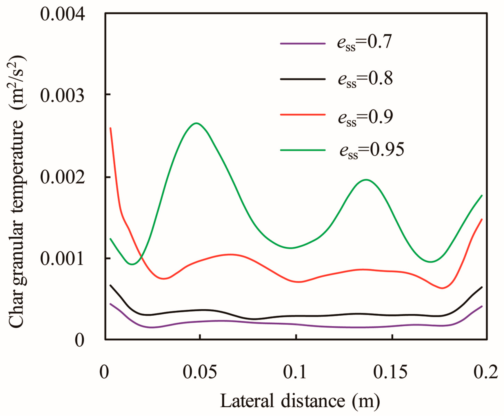
Granular temperature is a concept in the field of the kinetic theory of granular flow, and it is used for assessing fluctuating energy of the particles suspended in the gas flow. The lateral profiles of the time-averaged granular temperature of the flotsam at a height of 0.153 m are shown in Figure 10. When the restitution coefficient is no more than 0.9, the granular temperature of the flotsam closer to the wall is high and decreases towards the central region of the bed. Meanwhile, the curve becomes almost flat at the center of the bed. However, for the case of ess = 0.95, at the center of the bed, the curve is no longer flat. Two peaks of granular temperature can be found, which is related to the big values of the axial velocity, as shown in Figure 4 and Figure 9. With restitution coefficient increases, the values of the granular temperature increase, since there is less dissipation of the randomly fluctuating kinetic energy of particles. For a restitution coefficient below than 0.9, the granular temperature increases slightly. However, the granular temperature increases dramatically when the restitution coefficient increases from 0.9 to 0.95, especially for the center region of the bed.
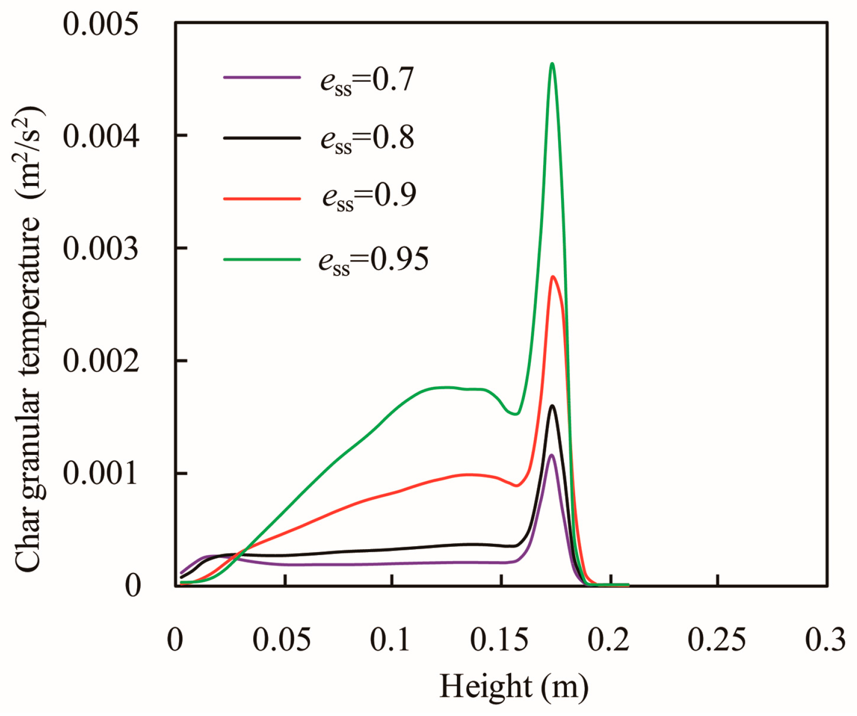
Figure 11 presents the axial profiles of the time-averaged granular temperature of the flotsam. In the region of the gas-solid interface, the granular temperature is very high, due to the collapse of bubbles and granular splash [27]. The value of granular temperature increases as the restitution coefficient increases. When the restitution coefficient increases from 0.7 to 0.8, the granular temperature along the axial direction increases slightly. However, with increase in restitution coefficient from 0.8 to 0.9, the granular temperature at the top of the bed increases obviously. Due to the similar flow patterns for the flotsam and jetsam, it can be seen than the effects of the restitution coefficient with different values on the granular temperature are also different.
4.4. Distribution of Particle Volume Fraction
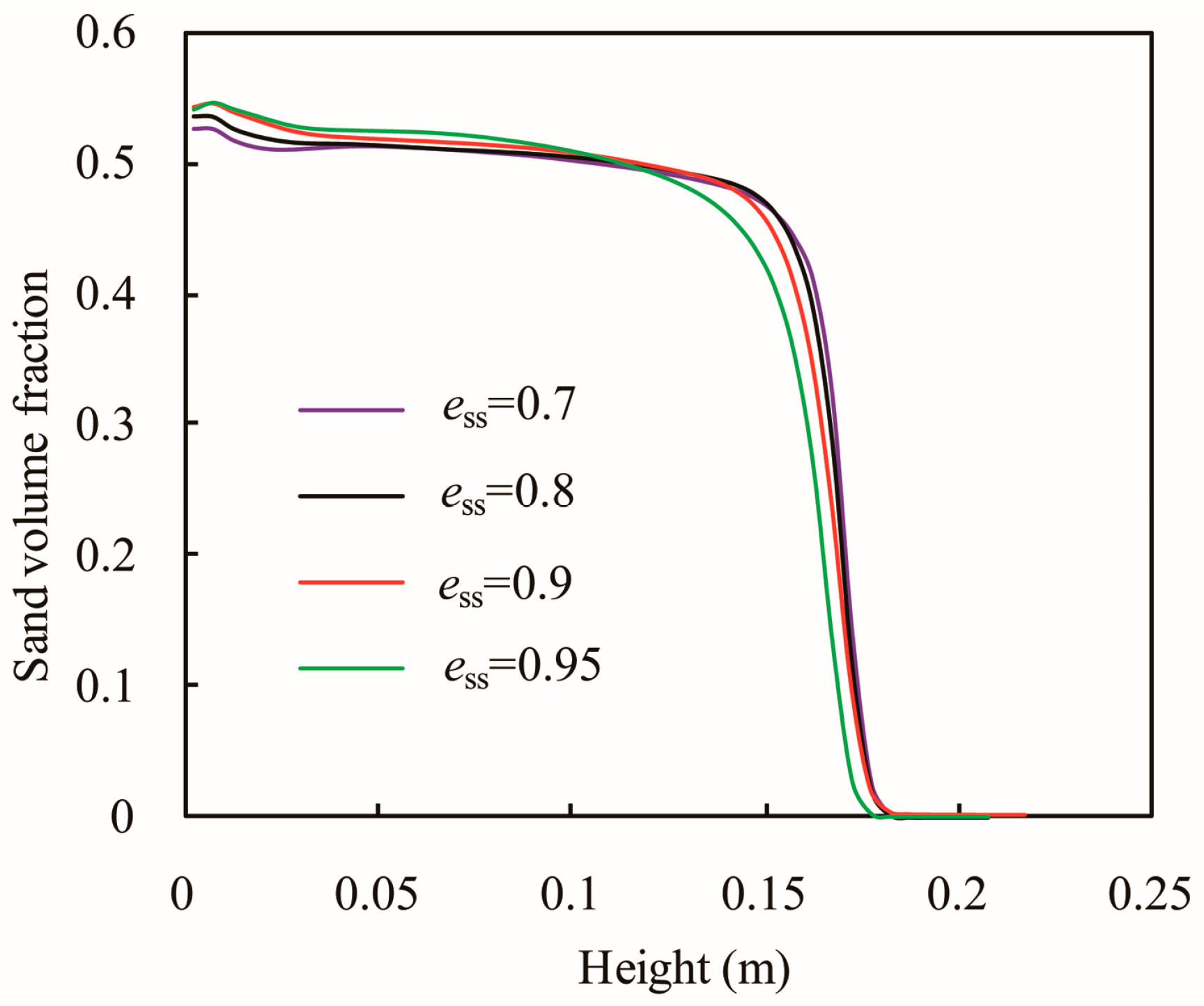
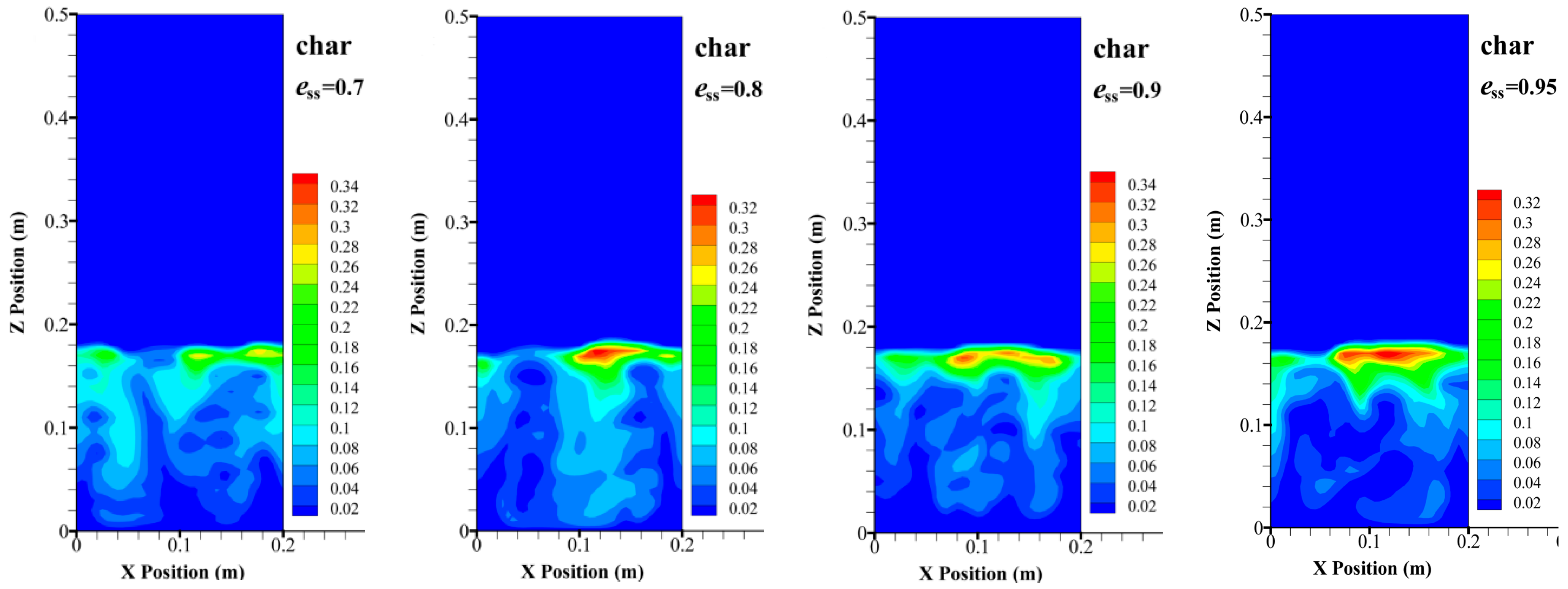
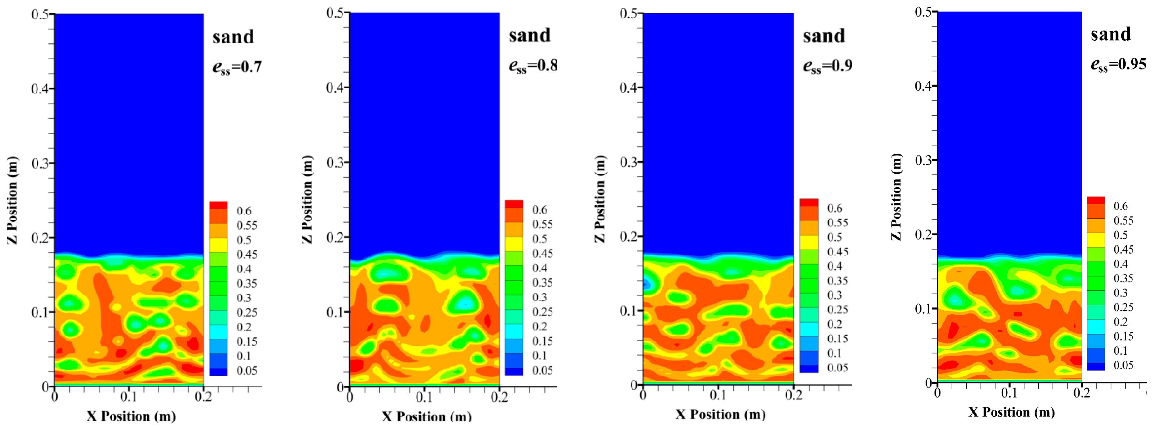
The effects of restitution coefficient on the instantaneous volume fraction of char and sand particles are shown in Figure 12 and Figure 13, respectively. Closer to the gas-solid interface, the volume fraction of sand particles is relatively low, which is just the opposite of the value of the char particles. This shows that a strong segregation phenomenon exists in the fluidization process of a binary particle system. With increase in the restitution coefficient, more char particles accumulate at the top of the bed, which shows that the tendency of segregation is more remarkable.
More studies [26,28] are concerned with the distribution characteristics of jetsam, however, in the gasification process, the flotsam will react with gas. Hence, the study on distribution characteristics of flotsam is much more significant. Lateral distributions of the time-averaged volume fraction of the flotsam at a height of 0.153 m are plotted in Figure 14. For ess = 0.7, 0.8, and 0.9, the effect of the restitution coefficient on the volume fraction of the flotsam is not obvious, hence, the profiles are very similar. However, when the restitution coefficient increases to 0.95, the values of volume fraction increase dramatically.
The effect of the restitution coefficient on the distribution of char mass fraction in the axial direction is shown in Figure 15. The char mass fraction is defined as the ratio of the char mass corresponding to the specific height range to total char mass in the bed. With increase in restitution coefficient, the char mass fraction in the upper part of the bed gradually increases, whereas the char mass fraction in the lower part of the bed decreases. In the case of ess = 0.95, the predicted profile well fits the experimental result. In the binary particles system with less difference between particles in density or volume fraction [12], they found that there was a small difference between the simulation results and the experimental data only for low restitution coefficient such as 0.8. However, for the binary particles system with huge difference in density and volume fraction between particles, the predicted degree of segregation compared with experimental result may be too low, when a relatively small value of restitution coefficient is adopted. From Figure 15, it can be seen that the mass fraction profile of char particles along the height direction for ess = 0.95 is quite close to the experimental result.
Figure 16 presents the axial profiles of the time-averaged particle volume fraction of the jetsam. Initially, the particle volume fraction along the bed height shows a slight increase, due to the effect of the inlet gas, and then gradually decreases. Closer to the gas-solid interface, the particle volume fraction decreases more sharply. This shows that the splash zone formed by the collapse of bubbles is a small area, which is consistent with previous studies [29,30]. The result from Figure 16 shows that the restitution coefficient had little effect on the axial profile of the jetsam volume fraction.
There are some studies about the comparison of results between 2D simulation and 3D simulation in the rectangular fluidized bed for monoparticle flow. For a pseudo-2D fluidized bed [31], the result has shown that no major differences are observed between 2D and 3D simulations in predicting the mean pressure drop and bed expansion. Just for bubble diameter and rise velocity, the 3D simulations are better agreement with experiments than the corresponding 2D simulations, whereas, for bubble aspect ratio, the 2D simulation has a better agreement with the experimental data. Xie et al. [32] also used an Eulerian-Eulerian model to investigate the differences between 2D and 3D simulations of a rectangular fluidized bed. They found that for a bubbling fluidized bed a satisfactory qualitative agreement between 2D and 3D simulations is observed. Hence, for monoparticle flow, though 2D simulations have certain limitations, they can provide reasonable results compared to experimental observations. Meanwhile, due to the requirement for lower computational resources, 2D simulation is widely used. However, for a binary mixture system in the rectangular fluidized bed, there are few related studies. Geng et al. [33] investigated the difference between the results of 2D and 3D simulations for a binary mixture system in a pseudo-2D rectangular bubbling fluidized bed. The results showed that the flotsam (coal particles) is nearly constant along the height direction, which totally deviates from the experimental observation. This means that 2D simulation is not suitable for modeling a pseudo-2D fluidized bed, which is entirely different from the conclusion for monoparticle flow. They also found that when the thickness of the rectangular bed was larger than a critical value (20 mm in this study), 2D simulation can provide a reasonable result. To sum up, the difference between 2D simulation and 3D simulation might change with the composition of the particle system. For a binary particle system, the relationship between the critical value in the thickness direction of the rectangular bed and the dimension parameters of the bed or the flow parameters may be important, and how to determine the relationship may be a key task in a follow-up study.
5. Conclusions
In the present work, the effect of the restitution coefficient on the numerical results for a binary particles system in a bubbling fluidized bed with the huge difference between the particles in terms of density and volume fraction has been studied based on two-fluid model along with the kinetic theory of granular flow. The effect of the restitution coefficient on the particle velocity, particle flow patterns, and mass fraction distribution varies in the different regions of the bed. At the bottom of the bed, the restitution coefficient does not affect the flow characteristic of particles significantly. However, in the top region of the bed, due to the cumulative effect of the dissipation of granular energy, the restitution coefficient has an obvious influence on the flow characteristic of the particles.
With an increase in the restitution coefficient, the degree of segregation increases. However, it does not change linearly with the restitution coefficient. Considering the effect of the restitution coefficient on the degree of segregation and flow pattern of particles in the top region of the bed, the restitution coefficient can be categorized into two classes: restitution coefficients of 0.7 and 0.8 can be included in one class, whereas the restitution coefficients of 0.9 and 0.95 can be included in another class.
For a binary particles system with the huge density and volume fraction difference between the particles, two vortices at the bottom of the bed and two vortices at the top of the bed are observed in the flow pattern distribution. The time-averaged flow pattern of particles in this study is very different from the result obtained for the system with similar values between particles in density and volume fraction, in which only two vortices can be found in the entire region of the dense bed layer.
Author Contributions
Xinjun Zhao did the simulation and wrote the manuscript. Qitai Eri and Qiang Wang supervised the investigation and checked the model.
Conflicts of Interest
The authors declare no conflict of interest.
References
- Fan, X.; Yang, Z.; Parker, D.J. Impact of solid sizes on flow structure and particle motions in bubbling fluidization. Powder Technol. 2011, 206, 132–138. [Google Scholar] [CrossRef]
- Mohd Salleh, M.A.; Kisiki, N.H.; Yusuf, H.M.; Ab Karim Ghani, W.A.W. Gasification of Biochar from Empty Fruit Bunch in a Fluidized Bed Reactor. Energies 2010, 3, 1344–1352. [Google Scholar] [CrossRef]
- Liu, H.; Zhao, Y.; Ding, J.; Gidaspow, D.; Wei, L. Investigation of mixing/segregation of mixture particles in gas-solid fluidized beds. Chem. Eng. Sci. 2007, 62, 301–317. [Google Scholar]
- Coroneo, M.; Mazzei, L.; Lettieri, P.; Paglianti, A.; Montante, G. CFD prediction of segregating fluidized bidisperse mixtures of particles differing in size and density in gas-solid fluidized beds. Chem. Eng. Sci. 2011, 66, 2317–2327. [Google Scholar] [CrossRef]
- Sun, J.; Wang, J.; Yang, Y. CFD investigation of particle fluctuation characteristics of bidisperse mixture in a gas-solid fluidized bed. Chem. Eng. Sci. 2012, 82, 285–298. [Google Scholar] [CrossRef]
- Loha, C.; Chattopadhyay, H.; Chatterjee, P.K. Euler-Euler CFD modeling of fluidized bed: Influence of specularity coefficient on hydrodynamic behavior. Particuology 2013, 11, 673–680. [Google Scholar] [CrossRef]
- Bakshi, A.; Altantzis, C.; Bates, R.B.; Ghoniem, A.F. Eulerian–Eulerian simulation of dense solid–gas cylindrical fluidized beds: Impact of wall boundary condition and drag model on fluidization. Powder Technol. 2015, 277, 47–62. [Google Scholar] [CrossRef]
- Wang, Y.; Zou, Z.; Li, H.; Zhu, Q. A new drag model for TFM simulation of gas-solid bubbling fluidized beds with Geldart-B particles. Particuology 2014, 15, 151–159. [Google Scholar] [CrossRef]
- Johnson, P.C.; Jackson, R. Frictional-collisional constitutive relations for granular materials with application to plane shearing. J. Fluid Mech. 1987, 176, 67–93. [Google Scholar] [CrossRef]
- Chao, Z.; Wang, Y.; Jakobsen, J.P.; Fernandino, M.; Jakobsen, H.A. Derivation and validation of a binary multi-fluid Eulerian model for fluidized beds. Chem. Eng. Sci. 2011, 66, 3605–3616. [Google Scholar] [CrossRef]
- Bai, W.; Keller, N.K.G.; Heindel, T.J.; Fox, R.O. Numerical study of mixing and segregation in a biomass fluidized bed. Powder Technol. 2013, 237, 355–366. [Google Scholar] [CrossRef]
- Tagliaferri, C.; Mazzei, L.; Lettieri, P.; Marzocchella, A.; Olivieri, G.; Salatino, P. CFD simulation of bubbling fluidized bidisperse mixtures: Effect of integration methods and restitution coefficient. Chem. Eng. Sci. 2013, 102, 324–334. [Google Scholar] [CrossRef]
- Mostafazadeh, M.; Rahimzadeh, H.; Hamzei, M. Numerical analysis of the mixing process in a gas-solid fluidized bed reactor. Powder Technol. 2013, 239, 422–433. [Google Scholar] [CrossRef]
- Zhong, H.; Gao, J.; Xu, C.; Lan, X. CFD modeling the hydrodynamics of binary particle mixtures in bubbling fluidized beds: Effect of wall boundary condition. Powder Technol. 2012, 230, 232–240. [Google Scholar] [CrossRef]
- Xue, Q.; Heindel, T.J.; Fox, R.O. A CFD model for biomass fast pyrolysis in fluidized-bed reactors. Chem. Eng. Sci. 2011, 66, 2440–2452. [Google Scholar] [CrossRef]
- Askarishahi, M.; Salehi, M.-S.; Molaei Dehkordi, A. Numerical investigation on the solid flow pattern in bubbling gas–solid fluidized beds: Effects of particle size and time averaging. Powder Technol. 2014, 264, 466–476. [Google Scholar] [CrossRef]
- Sande, P.C.; Ray, S. Mesh size effect on CFD simulation of gas-fluidized Geldart A particles. Powder Technol. 2014, 264, 43–53. [Google Scholar] [CrossRef]
- Wang, Y.; Chao, Z.; Jakobsen, H.A. A sensitivity study of the two-fluid model closure parameters (β, e) Determing the main gas-solid flow pattern characteristics. Ind. Eng. Chem. Res. 2010, 49, 3433–3441. [Google Scholar] [CrossRef]
- Zhong, H.; Lan, X.; Gao, J.; Zheng, Y.; Zhang, Z. The difference between specularity coefficient of 1 and no-slip solid phase wall boundary conditions in CFD simulation of gas-solid fluidized beds. Powder Technol. 2015, 286, 740–743. [Google Scholar] [CrossRef]
- Lun, C.C.K.; Savage, S.B.; Jeffrey, D.J.; Chepurniy, N. Kinetic theories for granular flow: Inelastic particles in Couette flow and slightly inelastic particles in a general flow field. J. Fluid Mech. 1984, 140, 223–256. [Google Scholar] [CrossRef]
- Park, H.C.; Choi, H.S. The segregation characteristics of char in a fluidized bed with varying column shapes. Powder Technol. 2013, 246, 561–571. [Google Scholar] [CrossRef]
- Gelderbloom, S.J.; Gidaspow, D.; Lyczkowski, R.W. CFD Simulations of Bubbling/Collapsing Fluidized Beds for Three Geldart Groups. AIChE J. 2003, 49, 844–858. [Google Scholar] [CrossRef]
- Chen, J.; Yu, G.; Dai, B.; Liu, D.; Zhao, L. CFD simulation of a bubbling fluidized bed gasifier using a bubble-based drag model. Energy Fuels 2014, 28, 6351–6360. [Google Scholar] [CrossRef]
- Chao, Z.; Wang, Y.; Jakobsen, J.P.; Fernandino, M.; Jakobsen, H.A. Multi-fluid modeling of density segregation in a dense binary fluidized bed. Particuology 2012, 10, 62–71. [Google Scholar] [CrossRef]
- Verma, V.; Deen, N.G.; Padding, J.T.; Kuipers, J.A.M. Two-fluid modeling of three-dimensional cylindrical gas–solid fluidized beds using the kinetic theory of granular flow. Chem. Eng. Sci. 2013, 102, 227–245. [Google Scholar] [CrossRef]
- Zhong, H.; Lan, X.; Gao, J.; Xu, C. Effect of particle frictional sliding during collisions on modeling the hydrodynamics of binary particle mixtures in bubbling fluidized beds. Powder Technol. 2014, 254, 36–43. [Google Scholar] [CrossRef]
- Yang, S.; Luo, K.; Fang, M.; Fan, J. LES–DEM investigation of the solid transportation mechanism in a 3-D bubbling fluidized bed. Part II: Solid dispersion and circulation properties. Powder Technol. 2014, 256, 395–403. [Google Scholar] [CrossRef]
- Di Renzo, A.; Di Maio, F.P.; Girimonte, R.; Vivacqua, V. Segregation direction reversal of gas-fluidized biomass/inert mixtures—Experiments based on particle segregation model predictions. Chem. Eng. J. 2015, 262, 727–736. [Google Scholar] [CrossRef]
- Li, T.; Grace, J.; Bi, X. Study of wall boundary condition in numerical simulations of bubbling fluidized beds. Powder Technol. 2010, 203, 447–457. [Google Scholar] [CrossRef]
- Zhao, Y.; Lu, B.; Zhong, Y. Influence of collisional parameters for rough particles on simulation of a gas-fluidized bed using a two-fluid model. Int. J. Multiph. Flow 2015, 71, 1–13. [Google Scholar] [CrossRef]
- Asegehegn, T.W.; Schreiber, M.; Krautz, H.J. Influence of two- and three-dimensional simulations on bubble behavior in gas-solid fluidized beds with and without immersed horizontal tubes. Powder Technol. 2012, 219, 9–19. [Google Scholar] [CrossRef]
- Xie, N.; Battaglia, F.; Pannala, S. Effects of using two-versus three-dimensional computational modeling of fluidized beds. Powder Technol. 2008, 182, 1–13. [Google Scholar] [CrossRef]
- Geng, S.; Jia, Z.; Zhan, J.; Liu, X.; Xu, G. CFD modeling the hydrodynamics of binary particle mixture in pseudo-2D bubbling fluidized bed: Effect of model parameters. Powder Technol. 2016, 302, 384–395. [Google Scholar] [CrossRef]
Figure 1.
Schematic representation of the fluidized bed.
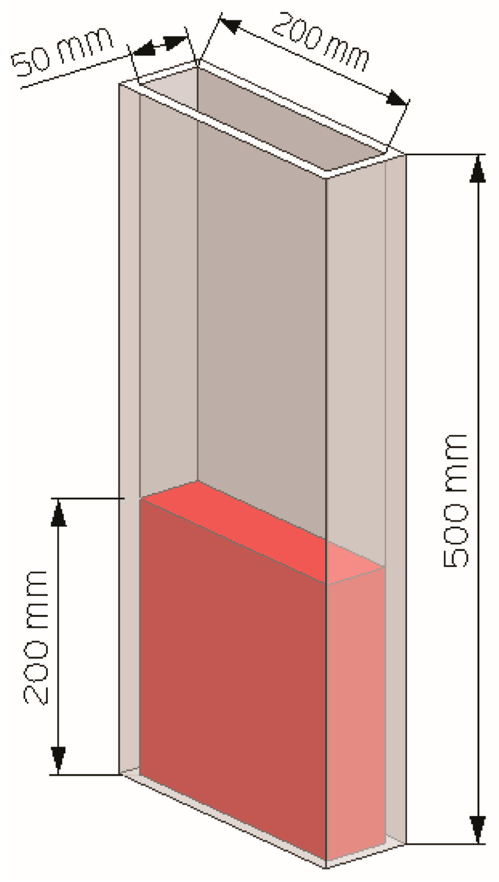
Figure 2.
Mesh geometry and coordinate system.
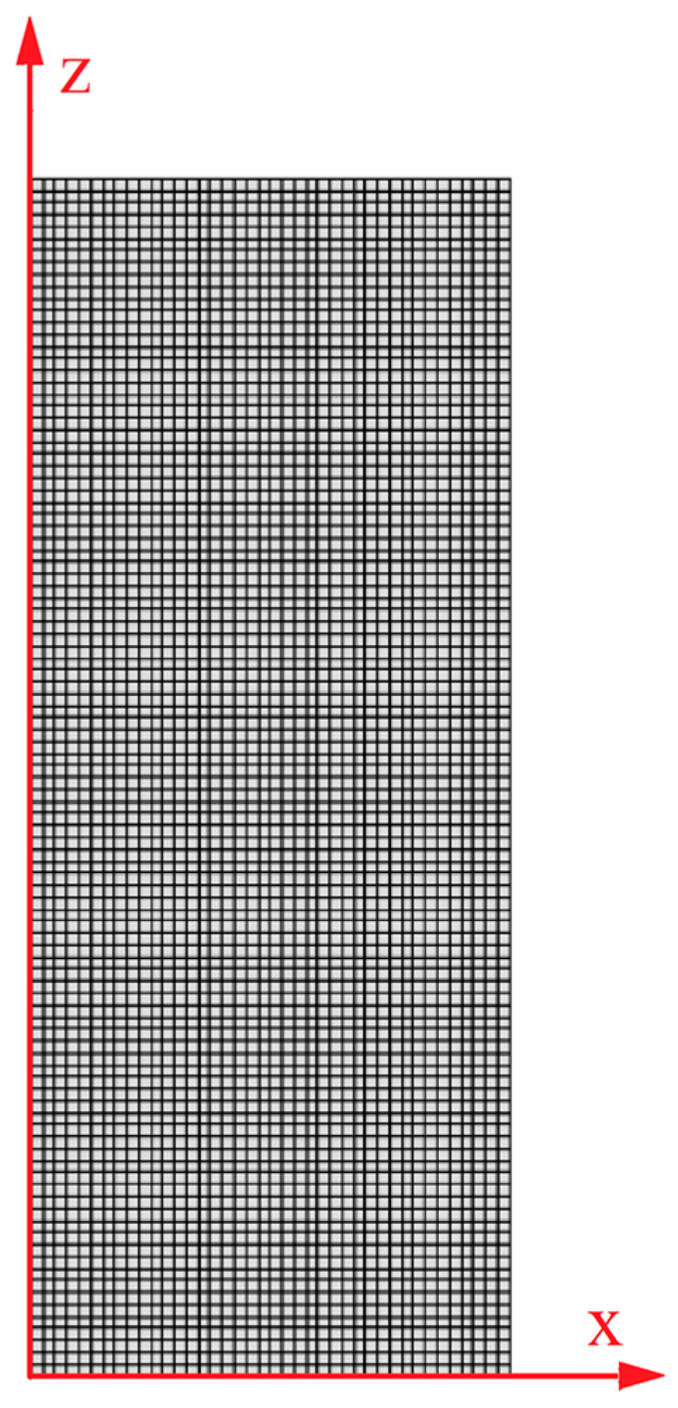
Figure 3.
Time profiles of the particle volume fraction in different layers along the height direction.
Figure 3.
Time profiles of the particle volume fraction in different layers along the height direction.
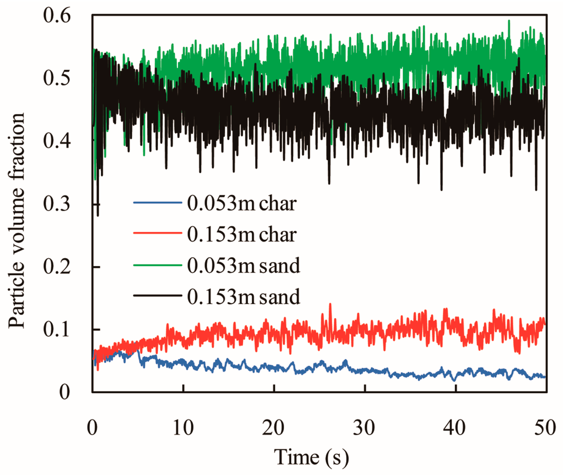
Figure 4.
Lateral profiles of the time-averaged axial velocity of the flotsam at Z = 0.153 m.

Figure 5.
Time-averaged particle velocity distribution of the flotsam for ess = 0.9 (the color legend represents the axial velocity of the particles).
Figure 5.
Time-averaged particle velocity distribution of the flotsam for ess = 0.9 (the color legend represents the axial velocity of the particles).

Figure 6.
Time-averaged particle velocity distribution of the jetsam for ess = 0.9 (the color legend represents the axial velocity of the particles).
Figure 6.
Time-averaged particle velocity distribution of the jetsam for ess = 0.9 (the color legend represents the axial velocity of the particles).
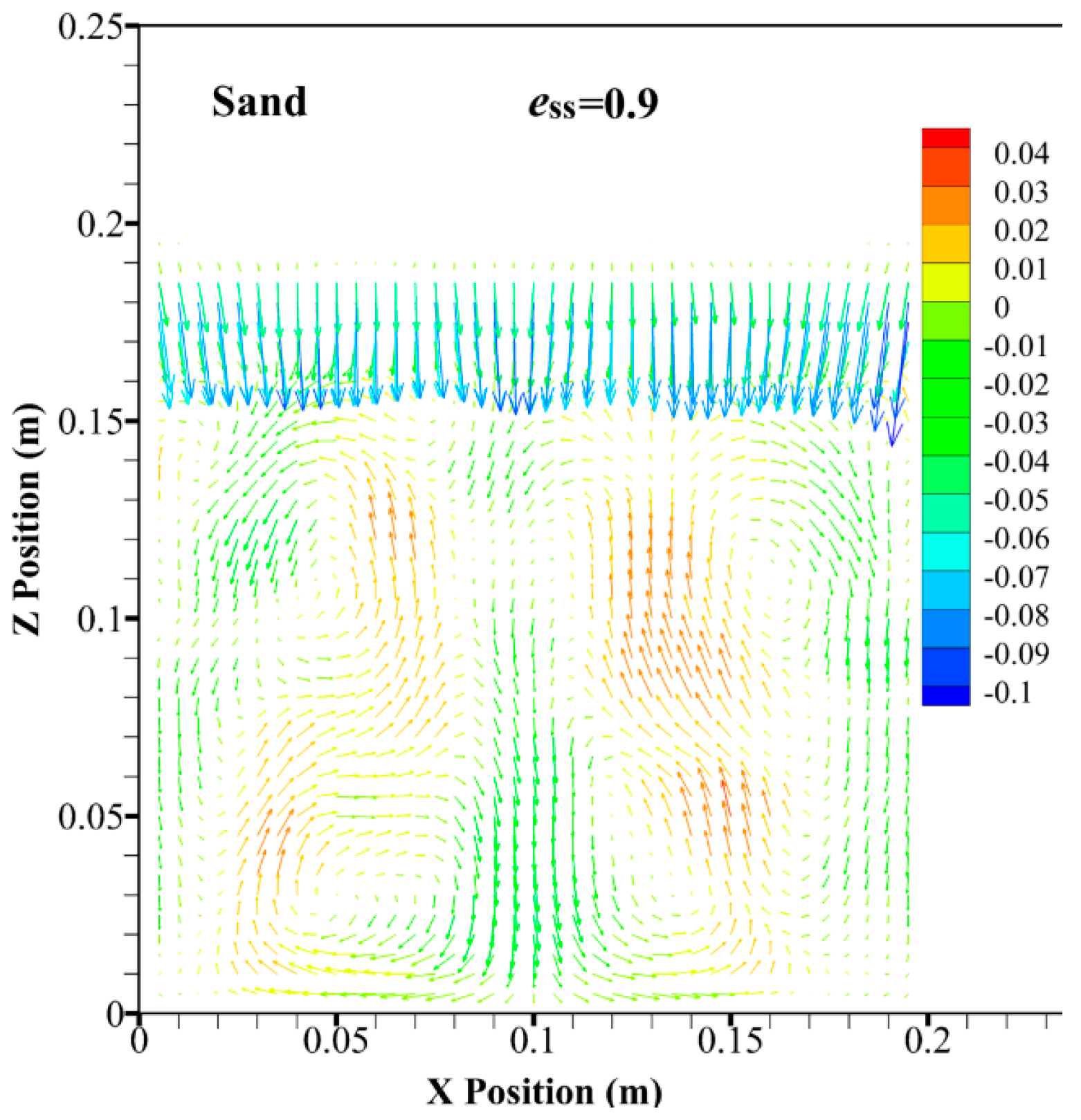
Figure 7.
Time-averaged particle velocity distribution of the flotsam for ess = 0.7 (the color legend represents the axial velocity of the particles).
Figure 7.
Time-averaged particle velocity distribution of the flotsam for ess = 0.7 (the color legend represents the axial velocity of the particles).

Figure 8.
Time-averaged particle velocity distribution of the flotsam for ess = 0.8 (the color legend represents the axial velocity of the particles).
Figure 8.
Time-averaged particle velocity distribution of the flotsam for ess = 0.8 (the color legend represents the axial velocity of the particles).

Figure 9.
Time-averaged particle velocity distribution of the flotsam for ess = 0.95 (the color legend represents the axial velocity of the particles).
Figure 9.
Time-averaged particle velocity distribution of the flotsam for ess = 0.95 (the color legend represents the axial velocity of the particles).
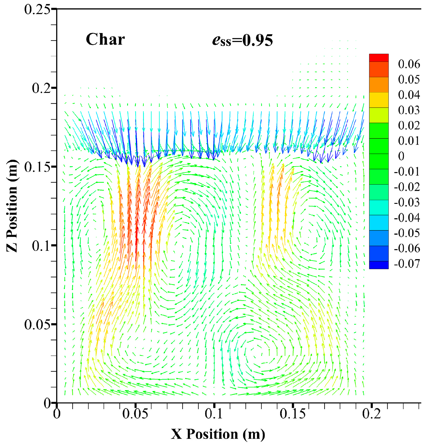
Figure 10.
Lateral profiles of the time-averaged granular temperature of the flotsam at Z = 0.153 m.
Figure 10.
Lateral profiles of the time-averaged granular temperature of the flotsam at Z = 0.153 m.

Figure 11.
Axial profiles of the time-averaged granular temperature of the flotsam.

Figure 12.
Distributions of instantaneous volume fraction of char particles.

Figure 13.
Distributions of instantaneous volume fraction of sand particles.

Figure 14.
Lateral profiles of the time-averaged particle volume fraction of the flotsam at Z = 0.153 m.
Figure 14.
Lateral profiles of the time-averaged particle volume fraction of the flotsam at Z = 0.153 m.
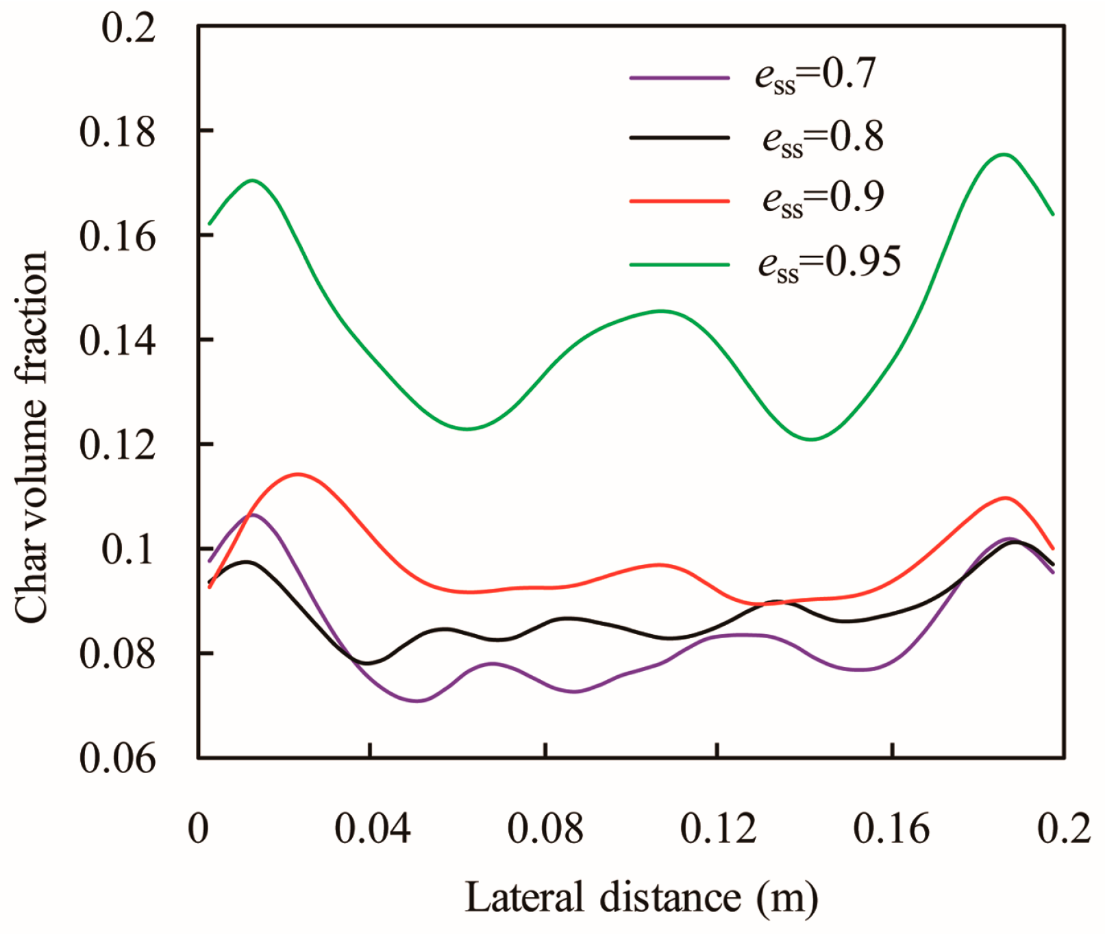
Figure 15.
Effect of restitution coefficient on the axial mass fraction profile of the flotsam.
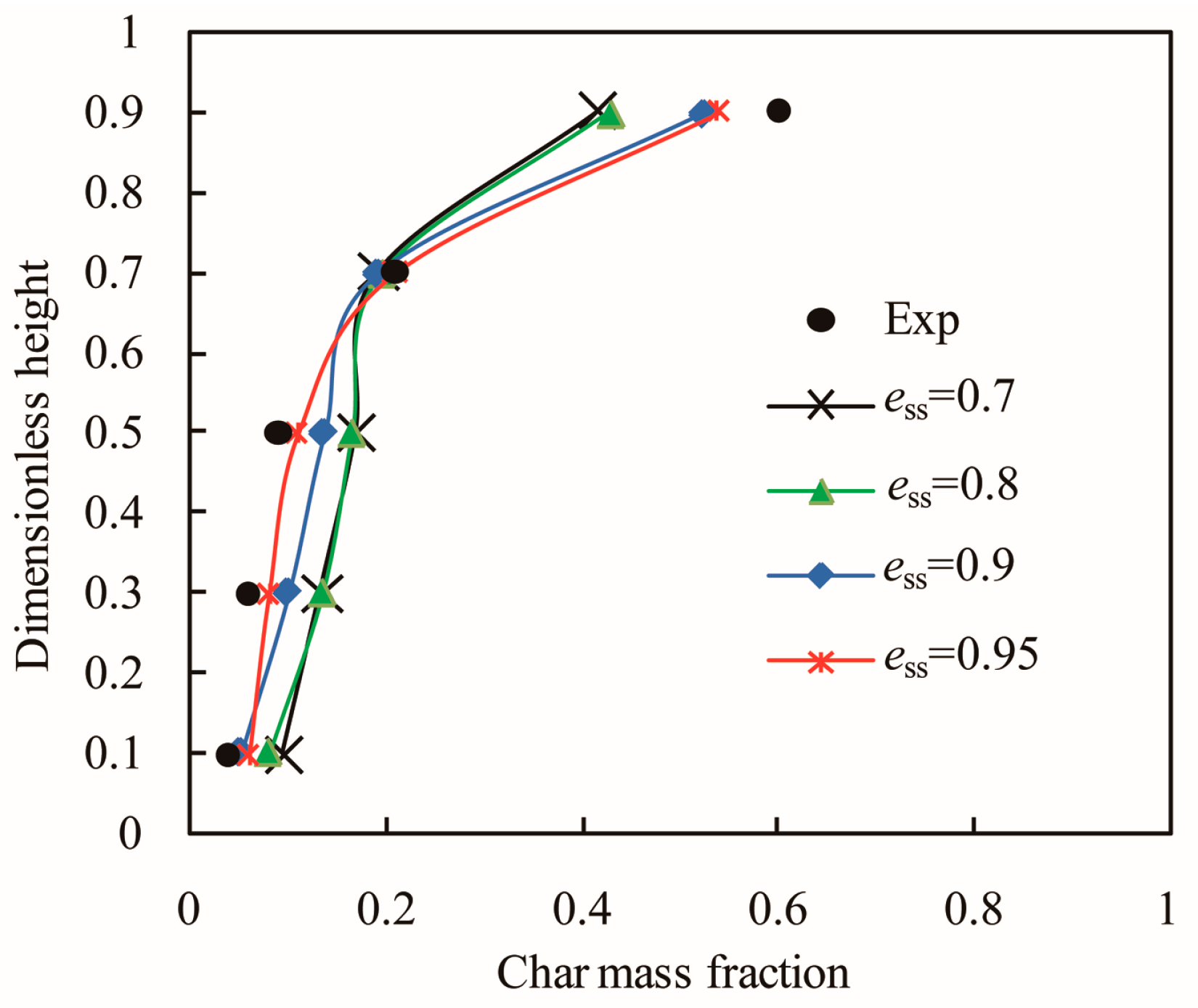
Figure 16.
Axial profiles of the time-averaged particle volume fraction of the jetsam.

Table 1.
Properties of particles.
| Particles | Mean Diameter (μm) | Void Fraction | Bulk Density (kg/m3) |
|---|---|---|---|
| Sand | 387 | 0.333 | 1590 |
| Char | 957 | 0.693 | 120 |
Table 2.
Summary of the simulation parameters.
| Parameter | Value or Model |
|---|---|
| Bed height (m) | 0.5 |
| Bed width (m) | 0.2 |
| Minimum fluidization velocity (m/s) | 0.14 |
| Superficial gas velocity (m/s) | 0.19 |
| Total particle weight (g) | Sand: 2000 Char: 40 |
| Particle volume fraction | Sand: 89% Char: 11% |
| Drag coefficient | Gidaspow |
| Granular viscosity | Syamlal-O’Brien |
| Granular bulk viscosity | Lun et al. |
| Restitution coefficient | ess = 0.7, 0.8, 0.9, 0.95 |
| Wall boundary condition | No-slip |
© 2017 by the authors. Licensee MDPI, Basel, Switzerland. This article is an open access article distributed under the terms and conditions of the Creative Commons Attribution (CC BY) license (http://creativecommons.org/licenses/by/4.0/).
Share and Cite
MDPI and ACS Style
Zhao, X.; Eri, Q.; Wang, Q. An Investigation of the Restitution Coefficient Impact on Simulating Sand-Char Mixing in a Bubbling Fluidized Bed. Energies 2017, 10, 617. https://doi.org/10.3390/en10050617
AMA Style
Zhao X, Eri Q, Wang Q. An Investigation of the Restitution Coefficient Impact on Simulating Sand-Char Mixing in a Bubbling Fluidized Bed. Energies. 2017; 10(5):617. https://doi.org/10.3390/en10050617
Chicago/Turabian StyleZhao, Xinjun, Qitai Eri, and Qiang Wang. 2017. "An Investigation of the Restitution Coefficient Impact on Simulating Sand-Char Mixing in a Bubbling Fluidized Bed" Energies 10, no. 5: 617. https://doi.org/10.3390/en10050617
Note that from the first issue of 2016, this journal uses article numbers instead of page numbers. See further details here.