
A Hybrid Dynamic System Assessment Methodology for Multi-Modal Transportation-Electrification


Thayer School of Engineering, Dartmouth College, 14 Engineering Drive, Hanover, NH 03755, USA
*
Author to whom correspondence should be addressed.
Energies 2017, 10(5), 653; https://doi.org/10.3390/en10050653
Submission received: 15 February 2017
/
Revised: 16 April 2017
/
Accepted: 4 May 2017
/
Published: 9 May 2017
(This article belongs to the Section F: Electrical Engineering)
Abstract
:In recent years, electrified transportation, be it in the form of buses, trains, or cars have become an emerging form of mobility. Electric vehicles (EVs), especially, are set to expand the amount of electric miles driven and energy consumed. Nevertheless, the question remains as to whether EVs will be technically feasible within infrastructure systems. Fundamentally, EVs interact with three interconnected systems: the (physical) transportation system, the electric power grid, and their supporting information systems. Coupling of the two physical systems essentially forms a nexus, the transportation-electricity nexus (TEN). This paper presents a hybrid dynamic system assessment methodology for multi-modal transportation-electrification. At its core, it utilizes a mathematical model which consists of a marked Petri-net model superimposed on the continuous time microscopic traffic dynamics and the electrical state evolution. The methodology consists of four steps: (1) establish the TEN structure; (2) establish the TEN behavior; (3) establish the TEN Intelligent Transportation-Energy System (ITES) decision-making; and (4) assess the TEN performance. In the presentation of the methodology, the Symmetrica test case is used throughout as an illustrative example. Consequently, values for several measures of performance are provided. This methodology is presented generically and may be used to assess the effects of transportation-electrification in any city or area; opening up possibilities for many future studies.
1. Introduction
1.1. The Emergence of Electrified Transportation
Electrified transportation, be it in the form of buses, trains, or cars are an emerging form of mobility. While electric trains have been an important form of urban transport for decades, it is the adoption of electric vehicles (EVs) as cars and buses that is set to expand the importance of electrified transportation in terms of distance traveled and energy consumed [1]. The shift to EVs as an enabling technology supports CO2 emissions reduction targets [2,3]. Relative to their internal combustion vehicle (ICV) counterparts, EVs are more energy efficient and consume less energy per unit distance [4]. They also have the added benefit of not emitting any carbon dioxide in operation and rather shift their emissions to the existing power generation fleet. As the power generation portfolio gains a greater penetration of renewable energy sources, the “well-to-wheel” carbon footprint of the EV approaches neutrality [5]. ICVs, in contrast, must emit CO2 not just for gasoline refining but also in the combustion of the fuel during transportation [2]. While the reduced well-to-wheel emissions of EVs drives renewable energy penetration, EVs have also been envisioned as an enabling technology to support renewable energy penetration [6]. These “Vehicle-to-Grid” applications provide demand side management of battery charging/discharging for enhanced control of the power grid balance [7,8,9,10,11].
Recently, this promise of EV-enabled CO2 emissions has gained further traction as technical, economic [12,13,14], and social barriers [8,15] have continually eased. First, despite continuing challenges in battery technology [16,17,18], a wide variety of battery chemistry options have emerged leading to greater capacity and subsequently vehicle ranges [19,20,21]. Second, fast chargers have been introduced into the market which allow 80% of the battery capacity to be charged in 30 min [9,22,23]. From an economic perspective, both plug-in hybrid EVs and battery-EVs show significant learning rates and cost improvements over time [14,24]. Finally, recent work has studied improvements to social barriers from the perspectives of public attitudes [25,26,27,28] and social transitions [4,8,15,29]. As a result, a number of optimistic market penetration and development studies have emerged for a wide variety of geographies [30,31,32,33,34,35,36]. Consequently, supportive policy options have taken root worldwide [25,37,38].
1.2. Infrastructure Considersations in Electrified Transportation
Despite these achievements, the true success of EVs depends on their successful integration with the infrastructure systems that support them. To that effect, EVs interact with three interconnected systems: the (physical) transportation system, the electric power grid [9], and their supporting information systems. In the transportation domain, such information systems are often called intelligent transportation systems [39,40,41,42,43,44,45,46], while in the electric domain they are often called energy management systems [47,48]. In this paper, their combined functionality is referred to as Intelligent Transportation-Energy System (ITES) [49,50]. Successful EV integration requires an assessment with regards to all three systems and their associated interdependencies.
With respect to the transportation system, EVs behave differently from ICVs in three regards. First, EVs typically have a travel range of approximately 150km [27]. Second, while ICVs can refuel in a matter of minutes, a typical EV may require 6-8 hours in order to fully recharge [51]. Finally, these two aspects of EVs can be further exacerbated by the geographic sparsity of charging stations causing drivers to go out of their way to charge [49]. These three aspects can lead to significantly altered user driving patterns and potentially different aggregate traffic behavior. From a private user perspective, the lack of perfect availability may be inconvenient. From a commercial user perspective, such driving patterns may erode the business case for adoption [25,49,52].
With respect to the electric power system, multiple aspects have to be considered for successful integration [53,54,55,56,57,58,59,60,61]. It is generally accepted that most EV adoption scenarios will not place excessive demands on the national power generation capacity [6,50]. Nevertheless, it is very likely that EV penetration can place excessive power demands on electric distribution which may exceed transformer ratings or cause undesirable line congestion and voltage deviations. These demands can be further exacerbated if EV adoption is dense geographically at the neighborhood length scale. Furthermore, if users adopt similar charging patterns, driven perhaps by similar work and travel lifestyles, the power required for charging can be temporally concentrated. Behr [62], Deutch and Moniz [22], and Markel [23] all state that one central challenge in the upgrade of the two physical systems is the EV charging infrastructure. EV charging stations, the analog of gasoline stations, serve as origin-destination nodes in a transportation system while simultaneously acting as load nodes in an electrical grid [63]. This coupling requires careful implementation [63,64]. In contrast, “online EVs” have been advanced as a new technology in which vehicles are inductive charged wirelessly while still in motion. This novel solution couples transportation links to electrical grid nodes in a new electrified transportation infrastructure that has the potential to assure vehicle availability [50].
Finally, with respect to information systems, Galus et al. [59], Junaibi [52], and Farid [50,63] state that the demands that EVs place on the physical infrastructure networks imply the need for informatic coordination. A parking lot operator, for example, may wish to use its energy management system to apply coordinated charging for its private EVs [65,66,67,68,69,70]. Furthermore, Gong et al. [71] states that a public transport operator might integrate the EV state of charge (SOC), its remaining available range, or even the real-time electricity spot price into its intelligent transportation system so as to co-optimize the dispatch of its transportation and charging services. Finally, electric utilities may wish to implement a vehicle-to-grid control scheme to optimize power grid balance, losses, congestion, and voltage deviations in the distribution management system [7,72,73]. In all, this information integration can be classified into five distinct ITES decisions summarized in Table 1 [50]. These functionalities, together, can serve to minimize operating costs, enhance power grid reliability, and enhance traffic congestion.
Traffic congestion and the effect it may have on the electric power grid requires dynamic modelling. A review of modeling approaches assessing the integration of electrified transportation has been found to, in general, use static analysis methods [74]. Although a static analysis may provide some insights into impacts of electrification, it does not acknowledge the interdependence of vehicles within a transportation system and how this would translate to grid impacts.
1.3. Original Contribution and Scope
This papers contributes a hybrid dynamic system assessment methodology for multi-modal transportation. It represents a natural evolution of the method originally developed in [75]. At the heart of the assessment methodology is the recently developed hybrid dynamic system (mathematical) model for multi-modal transportation electrification [63]. Such a system is called a transportation-electricity nexus (TEN).
Definition 1.
The usage of the TEN model facilitates the identification of input data, system structure, system behavior, decision variables, and output data relevant to the TEN. The mathematical model also facilitates the presentation of the methodology in a general fashion which furthermore facilitates its application on newly planned as well as existing infrastructure. Given the emergence of EVs in transportation electrification, the methodology inclines towards supporting EV integration studies. However, given that the underlying mathematical model is multi-modal, the methodology is viewed as such as well. The research towards this methodology is conducted by first investigating the most recent published EV integration studies; Second, the most appropriate methods to conduct such a study were analyzed, and subsequently extended to incorporate dynamic decision-making and performance measures. To illustrate the concepts explained in the paper, the Symmetrica test case [76] is used as an example throughout. The methodology is validated through a simulation of the Symmetrica test case with 50% adoption of plug-in EVs.
This methodology, to our knowledge, is the first of EV integration studies that presents a dynamic model. It takes into account the dynamic behavior present in any transportation system. This is a significant development from the methodologies within published literature, as generally static analysis is used [74]. The importance of such an assessment methodology can be understood by analogy from the precedent of renewable energy integration. At first, the integration of solar PV and wind energy was viewed from the perspective of small demonstration projects that had little or no effect on holistic power grid performance. As desired penetration rates grew into double-digit percentages, many renewable energy integration (case) studies [78,79,80,81,82] were developed; often with inconsistent methodological formulations. This work seeks to develop this methodological foundation for electrified transportation as it becomes an integral part of the coming sustainable energy transition.
1.4. Paper Outline
2. Transportation Electrification Assessment Methodology
This section forms the body of the paper and presents the transportation electrification assessment methodology. After a brief overview of the methodology in Section 2.1, Section 2.2 establishes the TEN structure, Section 2.3 presents the behavior of the TEN, Section 2.4 presents the ITES decision-making within the TEN dynamic system, and Section 2.5 presents performance measures to assess the performance of the TEN. As mentioned in Section 1.3, the methodology relies on a hybrid dynamic system model for multi-modal transportation electrification [63].
2.1. Overview
To begin the assessment methodology, Definition 1 of a TEN can be depicted graphically as in Figure 1. From a structural perspective, it consists of a transportation topology, a power system topology and a charging topology that couples them energetically and spatially. Each of these has their dynamic behaviors. For example, the transportation system may have mesoscopic or microscopic traffic behaviors [83,84]. It responds to exogeneous use case driven traffic demand in the form of itineraries that vehicles take over the course of the day [85]. The power system obeys Kirchoff’s Laws through power flow analysis [85]. It responds to exogeneous power demands (unrelated to transportation). The charging system draws electricity from the power system to charge vehicles in the transportation system. The structure and dynamics of such a TEN has been studied in detail as a hybrid dynamic model [63]. These physical dynamics also respond to ITES decision-making. The types of decisions have been identified in Table 1. While these decisions are spatially and energetically coupled, they may be taken in an integrated or independent fashion depending on the circumstances of the system being studied. Such decisions send signals from the ITES functionality down to the TEN’s physical system. Furthermore, such decisions can be conducted statically in an open-loop fashion or dynamically in a closed-loop fashion where the states and outputs of the physical dynamics are taken into account in the decision making. For example, dynamic routing [86] can be distinguished from static routing in that the former may take into account traffic congestion to optimize travel time. The presence of optimization objectives (e.g., travel time) suggests that the states and output of the TEN can be used to calculate performance measures of interest.
Consequently, the transportation electrification assessment methodology executes a numerical simulation of the TEN as a hybrid dynamic mathematical model [63] with its integrated ITES [49,50] within an operations time scale. This methodology requires four steps:
- (1)
- Establish the TEN structure.
- (2)
- Establish the TEN behavior.
- (3)
- Establish the TEN ITES decision-making.
- (4)
- Assess the TEN performance by numerical simulation.
Each of these steps is discussed in the following associated subsections. To facilitate the general discussion, each step is also illustrated using the Symmetrica test case [76]. It consists of a multi-modal electrified transportation system topology, an electric power topology, and activity-based use case data that spans transportation and charging [76].
2.1.1. Methodology
The first step in the assessment methodology is to establish the TEN’s physical structure. In transportation and power systems, graph theoretic models [87,88,89] are often proposed as a modeling analytical framework. A graph (be it directed or undirected) consists of nodes B and edges E. In transportation systems, the nodes often physically represent intersections and stations while edges represent roads, rails or transportation routes [85,86,90,91,92]. In power systems, the nodes often physically represent generators, substations, and loads while the edges represent the power lines [93,94]. The relationships between these nodes and edges are then analyzed using incidence and adjacency matrices. Despite its strength in modeling individual engineering systems, graph theory has significant limitations when two network systems are connected together. A recent review on multi-layer networks shows that such models often place limiting assumptions on how the networks may be coupled together [95]. From a practical electrified-transportation engineering perspective, such modeling limitations would constrain the charging topology in a TEN. To overcome this challenge, TEN’s structure is modeled using Axiomatic Design for Large Flexible Engineering Systems [96,97,98,99] as a type of hetero-functional graph theory. Its advantage relative to more traditional graph theoretic works has been previously motivated [63,98,99].
Definition 2.
The establishment of the TEN’s structure is captured in an LFES Knowledge Base.
Definition 3.
Essentially, the system knowledge base itself forms a bipartite graph which maps the set of system processes to their resources. Each filled element in the system knowledge base is called a structural degree of freedom and their number describes how many “capabilities" exist in the system [96,97,98]. Axiomatic Design for LFES also classifies system processes [96,97,98] into three varieties: transformation , transportation , and holding. It also classifies resources into three varieties: transforming resources , independent buffers , and transporting resources . Table 2 identifies the various types of system processes and resources in a TEN [96,97,98]. In order to construct the TEN knowledge base, the knowledge bases for the electrified transportation system and the electric power system must first be constructed. An overview of this process is presented here and the interested reader is referred to [63] for further mathematical details.
2.2. Establish TEN Structure
The system processes and resources in an electrified transportation system are similar to what one might expect for a conventional transportation system. As highlighted in Table 2, the main difference is the introduction of charging processes that occur while a vehicle is being transported from one location to another (not necessarily distinct) location.
Definition 4.
In electrified transportation systems, [50] where:
- —null charging does not change the EVs SOC.
- —discharge the EV SOC to the EV’s propulsion system.
- —charge the EV SOC by wire.
- —charge the EV SOC wirelessly.
Conventional stations effectively implement while conventional roads implement . Charging stations are capable of regardless of whether they are simply charging or implementing more advanced “vehicle to grid” technology [7,8,9]. The electrified roads associated with online EVs [102,103,104,105,106] are capable of .
This definition of the system processes and resources in the electrified transportation system allows the definition of the associated knowledge base [63]:
where:
where , and are smaller knowledge bases that reflect transformation, transportation, and charging functionality [63]. The ⊗ and · are the Kronecker and Hadamard products respectively and the notation reflects a column vector of ones of length n [96,97,98]. In effect, the electrified transportation system knowledge base is able to distinguish a collectively exhaustive and mutually exclusive set of processes out of the feasible combinations of processes and resources. For example, these can include “staying in place at a charging station while charging by wire” or “moving from to while charging wirelessly in online EV” [50,63].
The construction of an electric power system knowledge base follows similarly. Table 2 presents the system’s processes and resources [63]. Consequently, the electric power system knowledge base is defined as [63]:
where:
where , and are smaller knowledge bases that reflect transformation, transportation, and holding functionality [63].
It recognizes that any resource in the electrified transportation knowledge base may potentially inject or withdraw power from the grid depending whether it is capable of either charging process (i.e., wirelessly charging or charging by wire). Also note that while electrified roads and rail lines appear as transportation resources in the electrified transportation system, they appear as transforming resources in the larger nexus system. The full mathematical derivation of the knowledge base(s) is available in [63].
2.2.1. Symmetrica Example
The Symmetrica test case [98] is now used as an example to illustrate how the TEN structure can be captured in the TEN knowledge base. As shown in Figure 2, it consists of interlinked electrified transportation system and electric grid topologies. The transportation topology consists of a 12 × 12 km grid with intersections at every kilometer. Five charging stations are placed in the city center at coordinates (4,4), (4,8), (8,4), (8,8), and (6,6). Additionally, the peripheral nodes represent home charging. Finally, 13 groups of 2 km × 2 km electrified road crosses are uniformly distributed across the area. The power grid topology is a modified version of the 201-bus distribution system test case [107,108]. This test case will be referred to at each step of the assessment methodology.
Even for a moderately-sized test case such as Symmetrica, the system knowledge base becomes quite tedious to write manually and automated approaches instead are required. Here, it is important to recognize that the system knowledge base is a quantitative representation of an allocated architecture [98]. Several systems engineering languages (e.g., UML/SysML) represent an allocated architecture graphically [109,110,111]. Automated approaches can be used to transform the graphical representation into a quantitative one.
Consider Figure 3. For simplicity of discussion, four resources have been extracted from the Symmetrica test case topology. On the left, they are represented as class blocks in UML/SysML. Node #1 is a charging station. It has two methods (or system processes), park and charging, at Node #1; with “Null Charging” or with “Charging by Wire” . Node #2 is a parking lot. Like the charging station, it has a parking process. Link #1 is an electrified road. It has a system process of Transport Vehicles from Node #1 to #2 with battery discharging . It also has the process “charge wirelessly” during the transportation between nodes. Similarly, Link #2 has two system processes in the opposite direction. Figure 3 on the right shows the associated portion of the TEN knowledge base. There are 16 rows to account for the four possible transportation processes combined with four possible charging processes. There are 4 columns; one for each of the classes mentioned above. The matrix is then filled with ones where there are feasible combinations of system processes and resources (i.e., structural degrees of freedom) [96,97,98]. This small subsection has 7 degrees of freedom. Naturally, the system knowledge base is highly sparse and must be computationally implemented as such [50].
2.3. Establish TEN Behavior
2.3.1. Methodology
The TEN knowledge base serves as a structural skeleton of the TEN behavior. As expected, this behavior consists of the behavior related to the electrified transportation system and that of the electric power system. Furthermore, as these systems include both continuous-time as well as discrete-event dynamics, it requires a hybrid dynamic model [63]. The full definition of the model is provided in Definition 5 below. It assumes sufficient background in graph theory [87,88,89], timed Petri nets [112,113,114], microscopic traffic simulation [83,84,115] and power system dynamics [47] which is otherwise obtained from the provided references. Full mathematical details of the development of the hybrid dynamic model is presented in [63]. Its essential features are highlighted here.
Definition 5.
TEN hybrid dynamic model: A 10-tuple where:
- is the set of timed Petri net places. It represents transportation independent buffers (e.g., stations & intersections).
- is the set of timed Petri net discrete events. It represents the structural degrees of freedom (as defined in the previous section).
- is the set of arcs represented as the difference of two incidence matrices. It represents the logical relationship from the events to the places and from the places to the events.
- is the weighting function on the arcs. if and only if .
- is the timed Petri net discrete state vector for all discrete event times k.
- is the discrete state Petri-net transition function (Equation (7)).
- is a binary vehicle firing matrix for all discrete event times k.
- is a continuous-time state vector representing the kinematic and electric state of the TEN.
- is a set of invariant conditions [112] which associates a discrete state Q to an interval of X and within which X and must remain in order to also remain in the discrete state Q.
The state vectors and represent the number of vehicles at a Petri net place or undergoing a timed Petri net transition respectively [63]. The incidence matrices and are derived from the TEN knowledge base, and the firing vectors and are derived from the vehicle firing matrix [63].
The continuous time functions are classified into differential equation of the electrified transportation system and algebraic equations of electric power system [63]. The differential equations of the transportation system are implemented in state space form [63]:
They represent microscopic traffic dynamics of each vehicle traveling within the electrified transportation system [63]. In this regard, both free traffic flow and car-follower models have been previously studied [83,116,117]. are the well-known power flow analysis equations [47]:
where P is active power injection, Q is reactive power injection, V is bus voltage, and Y is the bus admittance matrix. Furthermore, the discrete state of the timed Petri-net discrete events is coupled to the active power injection in the electric power grid [63]:
where would represent the charging rate per vehicle of charging station or electrified road [63]. This hybrid dynamic mathematical model captures the discrete-event and continuous-time dynamic, describes the electrified transportation and electric power systems, and couples them together via the discrete state.
2.3.2. Symmetrica Example
The hybrid dynamic model takes on an intuitive character when applied to a test case such as Symmetrica. As in the previous section, a small portion of the Symmetrica transportation and power system topologies are taken for explanation. Consider Figure 4. It shows a Petri net with two places (shown as circles); one for each intersection in the transportation. It has seven discrete events (shown as rectangles) . These correspond to the seven degrees of freedom discussed in the previous subsection. The arcs between the places reflect the logical sequence of discrete states a vehicle may take and can be directly calculated from the knowledge base [63]. The weighting function W is restricted to one where arcs exist. The discrete state vector Q represents the number of vehicles at each Petri net place and transition.
In Figure 4, three vehicles are shown with distinct colors red, green, and blue. The Petri net transition function would then describe how these vehicle markings would evolve from discrete event k to the next. In the case of Figure 4, the red and blue vehicles were “fired” through transitions T5 and T6 respectively to mean both were transported from Node #1 to Node #2. The first with inductive charging and the other without. Naturally, the binary vehicle firing matrix indicates which vehicle is “fired” through a given transition at a given discrete event index k. Between discrete events, the continuous state evolves in time. The continuous electrified transportation system state describes as a minimum the position, velocity, and SOC of the vehicles going through the roads. It evolves by the continuous differential equation . The continuous electric power system state describes as a minimum the active and reactive power injections and voltages at the power system buses. It evolves by the continuous algebraic equation . Finally, it is important to recognize the continuous state adheres to a of applicability. Physically speaking, as vehicles reach the end of their respective road segments, or finish charging, the continuous state ceases to evolve, “pops" the vehicle out of its associated Petri net transition, and sends it to the downstream Petri net place. In such a way, the hybrid dynamic model describes the TEN behavior. This relatively complex behavior requires numerical simulation software to implement the mathematical model. Nevertheless, its primary advantage is that it supports an arbitrary TEN topology while leveraging established models of transportation and power system behavior.
2.4. Establish TEN Decision-Making
2.4.1. Methodology
Once the behavior of the TEN has been established, the focus shifts to assessing the ITES decision-making in the TEN. Here, it is important to distinguish between designing new ITES decision-making algorithms and simply assessing the decisions that already exist. While the former has been identified as an extensive area of future work [49,50,76], this work simply seeks to address the latter so as to describe TEN performance without change.
The TEN hybrid dynamic model presented in Definition 5 provides a structured approach for such an assessment. As expected, the decision-making can be classified into continuous-time and discrete-event decision-making. At a faster time scale, when the continuous time dynamics in Equation (10) are enhanced with real-time vehicle controller signals which affect the vehicles’ position, velocity, and SOC, they may be replaced with a new closed-loop real-time dynamic of the form:
Such an approach may be useful in the case when studying the integration of new EV concepts. For example, EVs with regenerative breaking increase the SOC as the vehicle decelerates. In this regard, the assessment resembles the assessment of different vehicle concepts under varying drive cycle conditions [118].
At a slower time scale, the timed Petri net in the hybrid dynamic model of the physical TEN system takes the binary vehicle firing matrix at each discrete event k as an input. Therefore, it may be viewed as the output of the ITES (as shown in Figure 1). Furthermore, as mentioned in the introduction, the ITES is assumed to take exogeneous use-case driven traffic demand in the form of itineraries that vehicles take over the course of the day [76]. Figure 5 shows two such home-work-home itineraries.
Such itineraries may be viewed as partial constraints on the values of the vehicle matrices over time depicting the sequence of origins and destinations of a given vehicle over the course of the day. With this understanding, the ITES decision-making can be viewed as a function that transforms into the much richer vehicle firing matrices c.
The ITES decision-making may also reflect dynamic decisions that take into the discrete-event state of the vehicles. In such a case:
The transportation-electrification assessment methodology can therefore be viewed as writing explicit mathematical decision-making models for Equations (14) and (15). While it is possible to imagine a single such mathematical model, the reality of transportation and electric power infrastructure is that several, perhaps entirely uncoordinated, decisions are taken. In that regard, the ITES decisions highlighted in Table 1 are now discussed in the context of both private and commercial uses cases.
Vehicle Dispatch: is defined here as when a vehicle should undertake a trip from origin to destination. As mentioned previously, this work assumes that the demand for trips between origins and destination is taken as input data and therefore acts as a decision constraint. Nevertheless, the timing and choice of vehicle can be decided. In the private use case, individuals may decide to expedite or postpone their departure so as to avoid congestion [119]. In the taxi use case, the choice of which taxi is dispatched when and where while optimizing battery capacity can enhance vehicle fleet utilization and therefore operating revenue [120]. This decision takes on a new dimension when considering that the demand for certain origin-destination trips can be shared within a single vehicle (e.g., Park & Ride) [121].
Route Choice: is defined as the set of roads and intersections that a vehicle should take along the course of an itinerary. The earliest route choice algorithms determined the shortest path with respect to distance for a given vehicle [122] and have since developed to include static as well as dynamic traffic assignment models [123,124,125]. Later the algorithms evolved to minimize time; taking into account road speed limits (and not just length). Dynamic route choice algorithms consider the congestion on the roads as a state. For EVs where the range may be limited, shortest path routing requires to also take into account locations of charging stations [126,127,128]. Regulations on high occupancy vehicles (HOV) can shift route choice behavior [37,38].
Charging Station Queue Management: is defined as when and where an EV should charge as queues develop in real-time. Because of their relatively lengthy charging time, EVs drivers can be informed with real-time state of charging queues. Instead of idly waiting to charge, drivers may change their choice of charging station. This choice is particularly important in the commercial use case after a given origin-destination trip has been completed. Charging station queues can also be managed in infrastructure planning. A location-sizing model to optimally allocate charging spots without exceeding waiting times has been proposed [129].
Coordinated Charging: is defined as when the vehicles at a given charging station should charge to meet drive departure times and power grid constraints. Typically, a charging station might work on a first-in-first-out heuristic. However, some vehicles in charging station parking lots may need to leave first. This presents a challenge when a given charging station is limited in the number of vehicles it can charge at a time. Finally, charging stations may wish to participate in demand response programs where dynamic prices can provide incentives to reshape charging load curves [9,53,54,55,56,57].
Vehicle-2-Grid Stabilization: is defined as when EVs are used as energy storage to enhance the stability of the power grid. Such a decision can be viewed as a generalization of coordinated charging in that it allows EVs to both inject electric power as well as withdraw it from the grid. This may be achieved at a slower time scale so as to be part of price-based demand response program. It may also occur as a real-time feedback control loop that enhances either the local voltage or frequency at the point of connection [9,53,54,55,56,57].
2.4.2. Symmetrica Example
The Symmetrica test case is meant to simulate a naive business-as-usual EV integration scenario. In recent years, there have been many EV pilots that integrate EVs without consideration for holistic TEN system performance and the need for enhanced ITES decision-making. As such, the ITES decisions in the Symmetrica test case are entirely uncoupled and reflect typical industrial practice. How each decision was implemented in simulation is now described sequentially. The traffic demand data found in [76] reflects the vehicle firing matrices in the hybrid dynamic model and is the output from the sequential execution of these five decisions.
Vehicle Dispatch: As expected from Equation (14), the generation of the Symmetrica vehicle firing matrices began with use-case driven traffic demand in the form of itineraries . For all vehicles, these represent a home-commute-work-commute-home use case, as a simplification of an average work day [76]. Returning to the transportation system topology in Figure 1, vehicles enter from the peripheral nodes, go to five work locations coinciding with charging stations and then after 8 hours return back to the periphery [76]. This input data has a spatial distribution so that all five work locations are equally important [76]. Meanwhile, the timing of commute departures was exponentially distributed around peak morning and afternoon timescite [76]. This input data was taken as exogeneous and no further vehicle dispatch decisions were made to change travel patterns.
Route Choice: While itinerary data specifies the location of the home-work-home use case, it does not specify the exact route taken and its associated firing vectors. Routing was performed by calculating shortest routes. Because there are many such routes, the routes were constrained so as to pass through the centers of the electrified road segments. Furthermore, vehicles having exactly the same home-work-home triplet were evenly distributed amongst the multiple paths that met these two criteria. In this way, no single road segment received an undue portion of the traffic.
Charging Station Queue Management: In keeping with the business-as-usual EV integration scenario, no effort was made to manage charging station queues. The sizes of the queues is effectively an emergent property.
Coordinated Charging: Similarly, the Symmetrica test case employed uncoordinated charging. As online EVs drive on electrified roads, they charge accordingly. Meanwhile, plugin-in EVs charge for a pre-calculated time as soon as they arrive at a charging station. The time spent charging was calculated based upon the expected value of lost charge during a commute. Each charging station has a capacity limit of simultaneously charging vehicles. This is 30 vehicles for the peripheral charging stations and 25 for the central charging stations. Together, these basic rules augment the vehicle route-itineraries to include charging functionality. This information is sufficient to generate a complete set of vehicle firing matrices.
Vehicle-2-Grid Stabilization: Similarly, no vehicle-2-grid stabilization decisions were made. Taken together, these five decisions provide all the necessary information to numerically simulate the TEN hybrid dynamic model.
To complete the simulation of ITES decision-making, energy management decisions for the electric power grid need to be included. For an uncoordinated charging scenario, the EVs present an aggregate charging power demand . This demand, taken in concert with the overall electric power demand , must be integrated into a electric power system energy management market [47]. The simplest of these is an economic dispatch that minimizes the production cost function :
subject to:
where power plant generation levels, are their associated cost levels, and and are the minimum and maximum generation levels respectively [47]. The economic dispatch is performed for each discrete event time k, dispatching generation for each demand level . Naturally, such an energy management market can be enhanced to include unit commitment, ramping limits, and transmission limits and losses [47]. In this uncoordinated charging scenario, the power system energy market acts “downstream” of EV charging and must make sure to dispatch sufficient electricity supply.
2.5. Assess the TEN Performance by Numerical Simulation
2.5.1. Methodology
Once the TEN dynamic behavior and the ITES decision-making have been established, the TEN’s performance can assessed by numerical simulation. In that regard, a number of quantitative performance measures are required. As infrastructure systems, both the electrified transportation system and the electric power system have many stakeholders each with their requirements and performance measures. While an exhaustive identification of performance measures is intractable here, several technical, economic and environmental concerns are highlighted as an overview on the subject.
The first group of performance measures address the electrified transportation infrastructure. These include congestion, queues, quality of service, asset utilization, and EV availability.
Definition 6.
Road Congestion : The number of vehicles on the conventional and electrified roads at a given discrete time k:
where is an appropriately sized constant row vector with ones corresponding to the elements associated with roads in .
Definition 7.
Parking Congestion : The number of parked vehicles at a given discrete time k:
where is an appropriately sized constant row vector with ones corresponding to the elements associated with parking lots in .
Definition 8.
Charging Congestion : The number of parked charging vehicles at a given discrete time k:
where is an appropriately sized constant row vector with ones corresponding to the elements associated with charging stations in .
Definitions 6–8 may be normalized by the total number registered vehicles to give relative measures of electrified transportation demand.
Definition 9.
System Queues : The number of queued vehicles at a given discrete time k:
where is an appropriately size column vectors of ones.
Definition 10.
Quality of Service : The fraction of time that the vehicle fleet is receiving a useful transportation service (i.e., motion, parking, charging). During these times, the vehicle fleet is not queued:
where K is the total number of discrete events over the course of the day.
Definition 11.
Resource (Asset) Utilization : Given a resource R, the fraction of a given resource’s capacity that is being utilized averaged over time:
where is a column vector containing the capacities of each of the structural degrees of freedom and is an appropriately sized row vector with ones corresponding to the elements associated with resource R.
Consequently, the asset utilization of the full electrified transportation system is:
Definition 12.
Vehicle Fleet Utilization : The fraction of time that the vehicle fleet is being driven:
Definition 13.
Vehicle Fleet Availability : The fraction of time that the vehicle fleet is neither charging nor queued:
In commercial and sharing use cases, the vehicle fleet utilization is relatively high limiting the time for charging. At some point, the vehicle fleet is effectively utilized to a maximum level of 100%.
Definition 14.
Effective Vehicle Fleet Utilization : The fraction of the available time that the vehicle fleet is being driven:
The second group of performance measures address the electric power system. Traditionally, these include balancing performance, line congestion, and voltage security limits [47]. CO2 emissions is added as an environmental measure.
Power System Balancing Performance: Several existing power system standards introduce balancing performance measures [48]. More recently, advancements in renewable energy integration studies suggest the standard deviation of imbalances normalized by peak load [130,131]. These values depend greatly on the design of power system energy markets and the quantities of different types of operating reserves [132,133,134]. This work assumes that the balancing performance is held constant as needed with a potential increase in the required operating reserves.
Power System Line Congestion: Power line rating places a physical limit on the amount of transferred active power P.
Definition 15.
Line Safety Criterion [75]: Given a set of lines, a given line i may have a line limit , over all discrete events K, the line safety criterion is defined as the average amount of excess active power in all the lines:
where:
Power System Voltage Security The IEEE Standard 519 [135] places bus voltage limits to be within 0.95 and 1.05 volts per unit.
Definition 16.
Bus Safety Criterion [75]: Over all discrete events K, the bus safety criterion is defined as the average amount of insufficient or excess voltage v in all the buses b:
where:
Power System CO2 Emissions: The additional CO2 emissions arises from their quantities before () and after () electrification:
The emissions associated with either scenario are calculated from the economic dispatch in the power system market. Each power plant i has a carbon emissions intensity curve which is a function of the amount of power generated . Consequently:
Naturally, the difference is caused by the difference between the load curve and the net load curve .
The third group of performance measures address the investment and operating costs as a result of coupling the transportation and electric power systems together.
TEN Investment Costs: From the previous discussion, the investment cost from electrified transportation comes from three sources: the purchase of EVs, the installation of charging infrastructure, the expansion of electric power generation, and distribution:
The purchase of EV is simply their number times their per unit cost :
The installation of charging infrastructure is the sum of charging stations and electrified roads weighted by their per unit costs ( and ):
Finally, the cost of additional power generation depends on the newly installed capacity and the per unit cost of new generation :
The quantity of required additional capacity is determined by simulation from the power system’s load duration curve before and after electrification [50]. Mathematically:
TEN Operating Costs: The additional operating costs from electrified transportation comes from two sources: the additional production costs in the energy markets, and the additional costs of maintaining power generation operating reserves:
The additional production costs in the energy markets is the optimal value of the objective function (Equation (16)) before and after electrification:
The additional costs of maintaining power generation operating reserves arises from their quantities before and after electrification:
3. Results: Symmetrica Test Case
The TEN performance of the Symmetrica test case is now discussed, for the scenario with 50% adoption of plug-in EVs. Two previous works [50,63] have already investigated this performance for two different scenarios, and the interested reader is encouraged to find more detailed discussion there. Here, the discussion first focuses on the performance measures described in the methodology and subsequently on the quantitative results. CO2 emissions, investment costs, and operating costs are not presented here as this would require additional data regarding electricity demand and power plant characteristics, which is outside the scope of this methodology paper.
3.1. Performance Measures
From the simulation data, the performance measures mentioned in Definitions 10–14 are calculated, and summarized in Table 3. The resource utilization and EV fleet utilization are particularly low as only two, relatively short, trips are undertaken between 6:00 a.m. and 8:00 p.m., requiring charging at only two moments during the day; the rest of the day all charging capacity is unused. Availability of the EV fleet is restricted by the time required to charge each EV, but remains particularly high indicating more effective use of each vehicle would be possible as is also indicated by the low effective utilization. Increased utilization can be achieved by car sharing strategies.
3.2. Quantitative Results
Figure 6 shows the results of the transportation electrification Symmetrica case with 50% plug-in EVs. It includes six subplots spanning the electrified transportation and electric power systems, each corresponding to a quantitative performance measure presented previously.
Road Congestion: In Figure 6a, the number of driving vehicles on a given road segment is shown with a distinct color, corresponding to Definition 6. Its shape reflects the decision-making for Symmetrica, as the traffic is dispatched in an exponentially distributed fashion in both the morning and the afternoon commute.
Parking Congestion: In Figure 6b, the number of parked vehicles at any given station is shown, corresponding to Definition 7. It rises sharply as the early-morning commute arrives at their destination, and then continues to rise over the course of a few hours.
Charging Congestion: This slow rise in the late afternoon is due to charging station congestion as shown in Figure 6c. Here, the quantity of stationary charging vehicles is shown, corresponding to Definition 8. The charging station capacity is quickly reached during the morning commute resulting in a built-up of queues.
System Queues: The size of these queues at each charging station are shown in Figure 6d. Here, the quantity of queued vehicles is shown, corresponding to Definition 9. Given this queue, the quality of service will not be 100%. The initial queue is due to the way Symmetrica data is presented, representing queuing before entering the cities from the periphery.
Feeder Lines Active Power: In Figure 6e, the active power in the three feeder lines are shown, corresponding to lines originating from bus 201. Depending on the limits on each line set in defining the line safety criterion, as introduced in Definition 15, these values may exceed limits. Here, the structure of the electrical grid and the charging station topology must be carefully rationalized so as to avoid underutilized and overutilized lines. In this particular case, the morning charging load is provided by just two of the three feeders but does not peak because of the saturation of charging stations. In the afternoon though, the charging activity peaks around 4:00 pm as all peripheral charging stations provide sufficient capacity, but is supplied almost exclusively by two feeder lines. Leveraging the topological flexibility of the electric distribution system may reduce reduce this peaking by dividing the total required power more evenly over all available feeder lines.
Terminal Bus Voltages: In Figure 6f, the bus voltage magnitudes of a selection of buses is shown upon completion of a power flow analysis at each discrete event k. The buses shown correspond to the terminals associated with the longest branches of the power system topology as shown in Figure 2. The safety criterion , as defined in Definition 16, is met in this case, as all bus voltages shown are within 0.95 and 1.05 volts per unit. Nonetheless, the effects of EV charging on the bus voltages coincide with the peak in charging demand in the afternoon, but show a different effect in response to the morning charging load. The morning voltages remain relatively stable throughout most of the charging. During the afternoon commute on the other hand, bus voltages are depressed much more substantially to almost 0.98 pu. While this is partially caused by the magnitude of the charging load, it is particularly amplified by the placement of several charging stations on the same feeder branch near its terminal. This raises questions as to the most appropriate nature of a power distribution system topology.
In conclusion, the ITES decision-making has a significant impact on the TEN’s holistic performance. Charging coordination, vehicle dispatch, charging station capacity and topology affect both the electrified transportation and electric power systems. New decision-making techniques are required to manage these simultaneous objectives.
4. Conclusions
This paper provides a new hybrid dynamic system assessment methodology for multi-modal transportation-electrification. Fundamentally, EVs interact with three interconnected systems: the (physical) transportation system, the electric power grid, and their supporting information systems. Coupling of the two physical systems essentially forms a TEN. The assessment methodology, presented here, provides clear and descriptive ways to establish the TEN structure, establish the TEN behavior, establish the TEN decision-making, and assess TEN performance. The transportation system model describes microscopic discrete-time traffic operations so as to study the kinematic and electric state of each EV at all times. The electric power system model studies balancing line and voltage performance. In this work, the Symmetrica test case has been used as an illustrative example. The presented hybrid dynamic system model lends itself to the design of performance measures to quantitatively assess technical, economic, and environmental characteristics. This methodology may be used to assess the effects of transportation-electrification in any city or area, as it is developed to be as general as possible, opening up possibilities for many future studies.
Author Contributions
Thomas J.T. van der Wardt and Amro M. Farid conceived and designed the methodology, Thomas J.T. van der Wardt performed the experiments, Thomas J.T. van der Wardt and Amro M. Farid wrote the paper.
Conflicts of Interest
The authors declare no conflict of interest.
References
- International Energy Agency. World Energy Outlook 2016—Executive Summary; Technical Report; OECD/IEA: Paris, France, 2016. [Google Scholar]
- Pasaoglu, G.; Honselaar, M.; Thiel, C. Potential vehicle fleet CO2 reductions and cost implications for various vehicle technology deployment scenarios in Europe. Energy Policy 2012, 40, 404–421. [Google Scholar] [CrossRef]
- Anair, D.; Mahmassani, A. State of Charge: Electric Vehicles’ Global Warming Emissions and Fuel-Cost Savings across the United States; Technical Report; Union of Concerned Scientists, Citizens and Scientists for Environmental Solutions: Cambridge, MA, USA, 2012. [Google Scholar]
- Soylu, S. Electric Vehicles—The Benefits and Barriers; Intech Open Access Publisher: Rijeka, Croatia, 2011; pp. 1–252. [Google Scholar]
- Litman, T. Comprehensive Evaluation of Transport Energy Conservation and Emission Reduction Policies; Victoria Transport Policy Institute: Victoria, BC, Canada, 2012. [Google Scholar]
- Kassakian, J.G.; Schmalensee, R.; Desgroseilliers, G.; Heidel, T.D.; Afridi, K.; Farid, A.M.; Grochow, J.M.; Hogan, W.W.; Jacoby, H.D.; Kirtley, J.L.; et al. Chapter 5: The Impact of Distributed Generation and Electric Vehicles. In The Future of the Electric Grid: An Interdisciplinary MIT Study; MIT Press: Cambridge, MA, USA, 2011; pp. 109–126. [Google Scholar]
- Kempton, W.; Tomić, J. Vehicle-to-grid power implementation: From stabilizing the grid to supporting large-scale renewable energy. J. Power Sources 2005, 144, 280–294. [Google Scholar] [CrossRef]
- Sovacool, B.K.; Hirsh, R.F. Beyond batteries: An examination of the benefits and barriers to plug-in hybrid electric vehicles (PHEVs) and a vehicle-to-grid (V2G) transition. Energy Policy 2009, 37, 1095–1103. [Google Scholar] [CrossRef]
- Su, W.; Rahimi-eichi, H.; Zeng, W.; Chow, M.Y. A survey on the electrification of transportation in a smart grid environment. IEEE Trans. Ind. Inform. 2012, 8, 1–10. [Google Scholar] [CrossRef]
- Ma, Y.; Zhang, B.; Zhou, X.; Gao, Z.; Wu, Y.; Yin, J.; Xu, X. An overview on V2G strategies to impacts from EV integration into power system. In Proceedings of the 2016 Chinese IEEE Control and Decision Conference (CCDC), Chongqing, China, 28–30 May 2016. [Google Scholar]
- Gago, R.G.; Pinto, S.F.; Silva, J.F. G2V and V2G electric vehicle charger for smart grids. In Proceedings of the 2016 IEEE International Smart Cities Conference (ISC2), Trento, Italy, 12–15 September 2016. [Google Scholar]
- Carlsson, F.; Johansson-Stenman, O. Costs and benefits of electric vehicles: A 2010 perspective. J. Transp. Econ. Policy 2003, 37, 1–28. [Google Scholar]
- Li, Z.; Ouyang, M. The pricing of charging for electric vehicles in China—Dilemma and solution. Energy 2011, 36, 5765–5778. [Google Scholar] [CrossRef]
- Weiss, M.; Patel, M.K.; Junginger, M.; Perujo, A.; Bonnel, P.; Grootveld, G.V. On the electrification of road transport—Learning rates and price forecasts for hybrid-electric and battery-electric vehicles. Energy Policy 2012, 48, 374–393. [Google Scholar] [CrossRef]
- Sierzchula, W.; Bakker, S.; Maat, K.; van Wee, B. The competitive environment of electric vehicles: An analysis of prototype and production models. Environ. Innov. Soc. Trans. 2012, 2, 49–65. [Google Scholar] [CrossRef]
- Pesaran, A.A.; Markel, T.; Tataria, H.S.; Howell, D. Battery requirements for plug-in hybrid electric vehicles—Analysis and rationale. In Proceedings of the 2007 23rd International Electric Vehicle Symposium, Anaheim, CA, USA, 2–5 December 2007. [Google Scholar]
- Kromer, M.A.; Heywood, J.B. Electric Powertrains: Opportunities and Challenges in the U.S. Light-Duty Vehicle Fleet; Technical Report; Massachuseets Institute of Technology: Cambridge, MA, USA, 2007. [Google Scholar]
- Manzetti, S.; Mariasiu, F. Electric vehicle battery technologies: From present state to future systems. Renew. Sustain. Energy Rev. 2015, 51, 1004–1012. [Google Scholar] [CrossRef]
- Lukic, S.M.; Cao, J.; Bansal, R.C.; Rodriguez, F.; Emadi, A. Energy storage systems for automotive applications. IEEE Trans. Ind. Electron. 2008, 55, 2258–2267. [Google Scholar] [CrossRef]
- Vazquez, S.; Lukic, S.M.; Galvan, E.; Franquelo, L.G.; Carrasco, J.M. Energy storage systems for transport and grid applications. IEEE Trans. Ind. Electron. 2010, 57, 3881–3895. [Google Scholar] [CrossRef]
- Fotouhi, A.; Auger, D.J.; Propp, K.; Longo, S.; Wild, M. A review on electric vehicle battery modelling: From Lithium-ion toward Lithium–Sulphur. Renew. Sustain. Energy Rev. 2016, 56, 1008–1021. [Google Scholar] [CrossRef]
- Deutch, J.; Moniz, E. Electrification of the Transportation System; Technical Report; Massachusetts Institute of Technology: Cambridge, MA, USA, 2010. [Google Scholar]
- Markel, T. Plug-in electric vehicle infrastructure: A foundation for electrified transportation. In Proceedings of the 2010 MIT Energy Initiative Transportation Electrification Symposium, Cambridge, MA, USA, 8 April 2010. [Google Scholar]
- Nykvist, B.; Nilsson, M. Rapidly falling costs of battery packs for electric vehicles. Nat. Clim. Chang. 2015, 5, 329–332. [Google Scholar] [CrossRef]
- Hadhrami, M.A.; Viswanath, A.; Junaibi, R.A.; Farid, A.M.; Sgouridis, S. Evaluation of Electric Vehicle Adoption Potential in Abu Dhabi; Technical Report; Masdar Institute of Science and Technology: Abu Dhabi, UAE, 2013. [Google Scholar]
- Zheng, J.; Mehndiratta, S.; Guo, J.Y.; Liu, Z. Strategic policies and demonstration program of electric vehicle in China. Transp. Policy 2012, 19, 17–25. [Google Scholar] [CrossRef]
- Skippon, S.; Garwood, M. Responses to battery electric vehicles: UK consumer attitudes and attributions of symbolic meaning following direct experience to reduce psychological distance. Transp. Res. D Transp. Environ. 2011, 16, 525–531. [Google Scholar] [CrossRef]
- Ahman, M. Government policy and the development of electric vehicles in Japan. Energy Policy 2006, 34, 433–443. [Google Scholar] [CrossRef]
- Van Bree, B.; Verbong, G.; Kramer, G. A multi-level perspective on the introduction of hydrogen and battery-electric vehicles. Technol. Forecast. Soc. Chang. 2010, 77, 529–540. [Google Scholar] [CrossRef]
- Schellenberg, J.A.; Member, M.J.S. Electric Vehicle Forecast for a Large West Coast Utility. In Proceedings of the 2011 IEEE Power and Energy Society General Meeting, Detroit, MI, USA, 24–28 July 2011. [Google Scholar]
- Yabe, K.; Shinoda, Y.; Seki, T.; Tanaka, H.; Akisawa, A. Market penetration speed and effects on CO2 reduction of electric vehicles and plug-in hybrid electric vehicles in Japan. Energy Policy 2012, 45, 529–540. [Google Scholar] [CrossRef]
- Burke, A. Present Status and Marketing Prospects of the Emerging Hybrid-Electric and Diesel Technologies to Reduce CO2 Emissions of New Light-Duty Vehicles in California; Institute of Transportation Studies: Davis, CA, USA, 2004. [Google Scholar]
- Parks, K.; Denholm, P.; Markel, T. Costs and Emissions Associated with Plug-In Hybrid Electric Vehicle Charging in the Xcel Energy Colorado Service Territory; Technical Report; National Renewable Energy Laboratory: Golden, CO, USA, 2007. [Google Scholar]
- Sikes, K.; Gross, T.; Lin, Z.; Sullivan, J.; Cleary, T.; Ward, J. Plug-In Hybrid Electric Vehicle Market Introduction Study Final Report; Technical Report; Sentech Inc.: Washington, DC, USA, 2010. [Google Scholar]
- Duvall, M.; Knipping, E. Environmental Assessment of Plug-In Hybrid Electric Vehicles; Technical Report; Electric Power Research Institute: Charlotte, NC, USA, 2007. [Google Scholar]
- Zhou, Y.; Wang, M.; Hao, H.; Johnson, L.; Wang, H. Plug-in electric vehicle market penetration and incentives: A global review. Mitig. Adapt. Strateg. Glob. Chang. 2015, 20, 777–795. [Google Scholar] [CrossRef]
- OCED-IEA-Anonymous. EV City Casebook: A Look at the Global Electric Vehicle Movement; Technical Report; Organisation for Economic Cooperation and Development/International Energy Agency: Paris, France, 2012. [Google Scholar]
- Tietge, U.; Mock, P.; Lutsey, N.; Campestrini, A. Comparison of Leading Electric Vehicle Policy and Deployment in Europe; International Council on Clean Transportation: Washington, DC, USA, 2016; Volume 49. [Google Scholar]
- U.S. Department of Transportation. Systems Engineering for Intelligent Transportation Systems: An Introduction for Transportation Professionals; Technical Report; U.S. Department of Transportation Federal Highway Administration Federal Transit Administration: Washington, DC, USA, 2007.
- TransCore. Integrating Intelligent Transportation Systems within the Transportation Planning Process; Technical Report; Federal Highway Administration: Washington, DC, USA, 1998.
- Meier, R.; Harrington, A.; Cahill, V. A Framework for Integrating Existing and Novel Intelligent Transportation Systems. In Proceedings of the IEEE Conference on Intelligent Transportation Systems, Vienna, Austria, 13–16 September 2005; pp. 650–655. [Google Scholar]
- Chowdhury, M.A.; Sadek, A.W. Fundamentals of Intelligent Transportation Systems Planning; Artech House: Boston, MA, USA, 2003; p. 190. [Google Scholar]
- Thill, J.C.; Rogova, G.; Yan, J. Evaluating benefits and costs of intelligent transportation systems elements from a planning perspective. Res. Transp. Econ. 2004, 8, 571–603. [Google Scholar] [CrossRef]
- Kanninen, B.J. Intelligent transportation systems: An economic and environmental policy assessment. Transp. Res. A Policy Pract. 1996, 30, 1–10. [Google Scholar] [CrossRef]
- He, J.; Zeng, Z.; Li, Z. Benefit evaluation framework of intelligent transportation systems. J. Transp. Syst. Eng. Inf. Technol. 2010, 10, 81–87. [Google Scholar] [CrossRef]
- Architecture-Development-Team. National Intelligent Transportation System Architecture: Executive Summary; Technical Report; Research and Innovation Technology Administration US Department of Transportation: Washington, DC, USA, 2012.
- Gómez-Expósito, A.; Conejo, A.J.; Cañizares, C. Electric Energy Systems: Analysis and Operation; CRC Press: Boca Raton, FL, USA, 2016. [Google Scholar]
- PJM-ISO. PJM Manual 3A: Energy Management System (EMS) Model Updates and Quality Assurance (QA); Technical Report; PJM Division, Operations Support; Operations Planning Department: Norristown, PA, USA, 2011. [Google Scholar]
- Al Junaibi, R.; Viswanath, A.; Farid, A.M. Technical Feasibility Assessment of Electric Vehicles: An Abu Dhabi Example. In Proceedings of the 2nd IEEE International Conference on Connected Vehicles and Expo, Las Vegas, NV, USA, 2–6 December 2013. [Google Scholar]
- Farid, A.M. Electrified Transportation System Performance: Conventional vs. Online Electric Vehicles. In Electrification of Ground Transportation Systems for Environment and Energy Conservation; Suh, N.P., Cho, D.H., Eds.; Springer: Berlin/Heidelberg, Germany, 2016; Chapter 22; pp. 1–25. [Google Scholar]
- Pointon, J. The Multi-Unit Dwelling Vehicle Charging Challenge. In Proceedings of the Electric Vehicles Virtual Summit 2012—The Smart Grid Observer, 13 September 2012; Volume 69. [Google Scholar]
- Junaibi, R.A. Technical Feasibility Assessment of Electric Vehicles in Abu Dhabi. Master’s Thesis, Masdar Institute of Science and Technology, Abu Dhabi, UAE, 2013. [Google Scholar]
- Pieltain Fernandez, L.; Roman, T.G.S.; Cossent, R.; Domingo, C.M.; Frias, P. Assessment of the Impact of Plug-in Electric Vehicles on Distribution Networks. IEEE Trans. Power Syst. 2011, 26, 206–213. [Google Scholar] [CrossRef]
- Lopes, J.A.P.; Soares, F.J.; Almeida, P.M.R. Integration of Electric Vehicles in the Electric Power System. Proc. IEEE 2011, 99, 168–183. [Google Scholar] [CrossRef]
- Qian, K.; Zhou, C.; Allan, M.; Yuan, Y. Modeling of Load Demand Due to EV Battery Charging in Distribution Systems. IEEE Trans. Power Syst. 2011, 26, 802–810. [Google Scholar] [CrossRef]
- Clement-Nyns, K.; Haesen, E.; Driesen, J. The Impact of Charging Plug-In Hybrid Electric Vehicles on a Residential Distribution Grid. IEEE Trans. Power Syst. 2010, 25, 371–380. [Google Scholar] [CrossRef]
- Dyke, K.J.; Schofield, N.; Barnes, M. The Impact of Transport Electrification on Electrical Networks. IEEE Trans. Ind. Electron. 2010, 57, 3917–3926. [Google Scholar] [CrossRef]
- Galus, M.; Zima, M.; Andersson, G. On integration of plug-in hybrid electric vehicles into existing power system structures. Energy Policy 2010, 38, 6736–6745. [Google Scholar] [CrossRef]
- Galus, M.D.; Waraich, R.A.; Noembrini, F.; Steurs, K.; Georges, G.; Boulouchos, K.; Axhausen, K.W.; Andersson, G. Integrating Power Systems, Transport Systems and Vehicle Technology for Electric Mobility Impact Assessment and Efficient Control. IEEE Trans. Smart Grid 2012, 3, 934–949. [Google Scholar] [CrossRef]
- Perujo, A.; Ciuffo, B. The introduction of electric vehicles in the private fleet: Potential impact on the electric supply system and on the environment. A case study for the Province of Milan, Italy. Energy Policy 2010, 38, 4549–4561. [Google Scholar] [CrossRef]
- Soares, J.A.; Canizes, B.; Lobo, C.; Vale, Z.; Morais, H. Electric Vehicle Scenario Simulator Tool for Smart Grid Operators. Energies 2012, 5, 1881–1899. [Google Scholar] [CrossRef]
- Behr, P. MIT Panel Says a Charging Infrastructure May Be a Bigger Roadblock for Electric Vehicles Than Technology; Scientific American: New York, NY, USA, 2011; pp. 1–6. [Google Scholar]
- Farid, A.M. A Hybrid Dynamic System Model for Multi-Modal Transportation Electrification. IEEE Trans. Control Syst. Technol. 2017, 25, 940–951. [Google Scholar] [CrossRef]
- Lam, A.Y.; Leung, Y.W.; Chu, X. Electric vehicle charging station placement: Formulation, complexity, and solutions. IEEE Trans. Smart Grid 2014, 5, 2846–2856. [Google Scholar] [CrossRef]
- Palensky, P.; Dietrich, D. Demand Side Management: Demand Response, Intelligent Energy Systems, and Smart Loads. IEEE Trans. Ind. Inform. 2011, 7, 381–388. [Google Scholar] [CrossRef]
- Sortomme, E.; Hindi, M.M.; MacPherson, S.D.J.; Venkata, S.S. Coordinated Charging of Plug-In Hybrid Electric Vehicles to Minimize Distribution System Losses. IEEE Trans. Smart Grid 2011, 2, 198–205. [Google Scholar] [CrossRef]
- Saber, A.Y.; Venayagamoorthy, G.K. Plug-in Vehicles and Renewable Energy Sources for Cost and Emission Reductions. IEEE Trans. Ind. Electron. 2011, 58, 1229–1238. [Google Scholar] [CrossRef]
- Gan, L.; Topcu, U.; Low, S. Optimal decentralized protocol for electric vehicle charging. In Proceedings of the IEEE Conference on Decision and Control and European Control Conference, Orlando, FL, USA, 12–15 December 2011; pp. 5798–5804. [Google Scholar]
- Erol-Kantarci, M.; Sarker, J.H.; Mouftah, H.T. Quality of service in Plug-in Electric Vehicle charging infrastructure. In Proceedings of the 2012 IEEE International Electric Vehicle Conference (IEVC), Greenville, SC, USA, 4–8 March 2012. [Google Scholar]
- Ma, Z.; Callaway, D.; Hiskens, I. Optimal Charging Control for Plug-In Electric Vehicles. In Control and Optimization Methods for Electric Smart Grids; Springer: Berlin, Germany, 2012; pp. 259–273. [Google Scholar]
- Gong, Q.; Li, Y.; Peng, Z.R. Optimal Power Management of Plug-in HEV with Intelligent Transportation System. In Proceedings of the 2007 IEEE/ASME International Conference on Advanced intelligent Mechatronics, Zurich, Switzerland, 4–7 September 2007. [Google Scholar]
- Andersen, P.H.; Mathews, J.A.; Rask, M. Integrating private transport into renewable energy policy: The strategy of creating intelligent recharging grids for electric vehicles. Energy Policy 2009, 37, 2481–2486. [Google Scholar] [CrossRef]
- Falvo, M.C.; Lamedica, R.; Bartoni, R.; Maranzano, G. Energy management in metro-transit systems: An innovative proposal toward an integrated and sustainable urban mobility system including plug-in electric vehicles. Electr. Power Syst. Rese. 2011, 81, 2127–2138. [Google Scholar] [CrossRef]
- Richardson, D.B. Electric vehicles and the electric grid: A review of modeling approachces, Impacts, and renewable energy integration. Renew. Sustain. Energy Rev. 2013, 19, 247–254. [Google Scholar] [CrossRef]
- Junaibi, R.A.; Farid, A.M. A Method for the Technical Feasibility Assessment of Electrical Vehicle Penetration. In Proceedings of the 7th Annual IEEE System Conference (SysCon), Orlando, FL, USA, 15–18 April 2013. [Google Scholar]
- Farid, A.M. Symmetrica: Test Case for Transportation Electrification Research. Infrastruc. Complex. 2015, 2, 9. [Google Scholar] [CrossRef]
- Viswanath, A.; Farid, A.M. A Hybrid Dynamic System Model for the Assessment of Transportation Electrification. In Proceedings of the 2014 IEEE American Control Conference, Portland, OR, USA, 4–6 June 2014. [Google Scholar]
- Farid, A.M.; Jiang, B.; Muzhikyan, A.; Youcef-Toumi, K. The Need for Holistic Enterprise Control Assessment Methods for the Future Electricity Grid. Renew. Sustain. Energy Rev. 2015, 56, 669–685. [Google Scholar] [CrossRef]
- Brouwer, A.S.; van den Broek, M.; Seebregts, A.; Faaij, A. Impacts of large-scale Intermittent Renewable Energy Sources on electricity systems, and how these can be modeled. Renew. Sustain. Energy Rev. 2014, 33, 443–466. [Google Scholar] [CrossRef]
- Holttinen, H.; Milligan, M.; Ela, E.; Menemenlis, N.; Dobschinski, J.; Rawn, B.; Bessa, R.J.; Flynn, D.; Gomez-Lazaro, E.; Detlefsen, N.K. Methodologies to Determine Operating Reserves Due to Increased Wind Power. IEEE Trans. Sustain. Energy 2012, 3, 713–723. [Google Scholar] [CrossRef]
- Holttinen, H.; Orths, A.; Abilgaard, H.; van Hulle, F.; Kiviluoma, J.; Lange, B.; O’Malley, M.; Flynn, D.; Keane, A.; Dillon, J.; et al. IEA Wind Export Group Report on Recommended Practices Wind Integration Studies; Technical Report; International Energy Agency: Paris, France, 2013. [Google Scholar]
- Ela, E.; Milligan, M.; Parsons, B.; Lew, D.; Corbus, D. The evolution of wind power integration studies: Past, present, and future. In Proceedings of the 2009 IEEE Power & Energy Society General Meeting (PES’09), Calgary, AB, Canada, 26–30 July 2009. [Google Scholar]
- Treiber, M.; Kesting, A. Traffic Flow Dynamics: Data, Models and Simulation; Springer: Heidelberg, Germany; New York, NY, USA, 2013; p. 503. [Google Scholar]
- Barcelo, J.; Kuwahara, M. Traffic Data Collection and Its Standardization; Springer: New York, NY, USA, 2008; p. 194. [Google Scholar]
- Zografos, K.G.; Androutsopoulos, K.N. Algorithms for Itinerary Planning in Multimodal Transportation Networks. IEEE Trans. Intell. Transp. Syst. 2008, 9, 175–184. [Google Scholar] [CrossRef]
- Pillac, V.; Gendreau, M.; Guéret, C.; Medaglia, A.L. A review of dynamic vehicle routing problems. Eur. J. Oper. Res. 2013, 225, 1–11. [Google Scholar] [CrossRef]
- Newman, M. Networks: An Introduction; OUP: Oxford, UK, 2009. [Google Scholar]
- Van Steen, M. Graph Theory and Complex Networks: An Introduction; Maarten van Steen: Enschede, The Netherlands, 2010; pp. 1–300. [Google Scholar]
- Lewis, T.G. Network Science: Theory and Applications; Wiley: Hoboken, NJ, USA, 2011; p. 512. [Google Scholar]
- Ip, W.H.; Wang, D. Resilience and Friability of Transportation Networks: Evaluation, Analysis and Optimization. IEEE Syst. J. 2011, 5, 189–198. [Google Scholar] [CrossRef]
- Zografos, K.G.; Androutsopoulos, K.N.; Spitadakis, V. Design and Assessment of an Online Passenger Information System for Integrated Multimodal Trip Planning. IEEE Trans. Intell. Transp. Syst. 2009, 10, 311–323. [Google Scholar] [CrossRef]
- Hame, L.; Hakula, H. Dynamic Journeying in Scheduled Networks. IEEE Trans. Intell. Transp. Syst. 2013, 14, 360–369. [Google Scholar] [CrossRef]
- Zimmerman, R.D.; Murillo-Sánchez, C.E.; Thomas, R.J. MATPOWER: Steady-state operations, planning, and analysis tools for power systems research and education. IEEE Trans. Power Syst. 2011, 26, 12–19. [Google Scholar] [CrossRef]
- Ash, J.; Newth, D. Optimizing complex networks for resilience against cascading failure. Phys. A Stat. Mech. Appl. 2007, 380, 673–683. [Google Scholar] [CrossRef]
- Kivelä, M.; Arenas, A.; Barthelemy, M.; Gleeson, J.P.; Moreno, Y.; Porter, M.A. Multilayer networks. J. Complex Netw. 2014, 2, 203–271. [Google Scholar] [CrossRef]
- Farid, A.M. Product Degrees of Freedom as Manufacturing System Reconfiguration Potential Measures. Int. Trans. Syst. Sci. Appl. 2008, 4, 227–242. [Google Scholar]
- Farid, A.M.; McFarlane, D.C. Production degrees of freedom as manufacturing system reconfiguration potential measures. Proc. Inst. Mech. Eng. B J. Eng. Manuf. 2008, 222, 1301–1314. [Google Scholar] [CrossRef]
- Farid, A.M. Static Resilience of Large Flexible Engineering Systems: Axiomatic Design Model and Measures. IEEE Syst. J. 2015, PP, 1–12. [Google Scholar] [CrossRef]
- Suh, N.P. Axiomatic Design: Advances and Applications; Oxford University Press: Oxford, UK, 2001. [Google Scholar]
- SE Handbook Working Group. Systems Engineering Handbook: A Guide for System Life Cycle Processes and Activities; International Council on Systems Engineering (INCOSE): San Diego, CA, USA, 2011; pp. 1–386. [Google Scholar]
- Friedenthal, S.; Moore, A.; Steiner, R. A Practical Guide to SysML: The Systems Modeling Language, 2nd ed.; Morgan Kaufmann: Burlington, MA, USA, 2011; p. 640. [Google Scholar]
- Ahn, S.; Kim, J.; Cho, D.-H. Wireless Power Transfer in On-Line Electric Vehicle. In Wireless Power Transfer, 2nd ed.; River Publishers: Aalborg, Denmark, 2012; p. 416. [Google Scholar]
- Jang, Y.J.; Ko, Y.D.; Jeong, S. Optimal design of the wireless charging electric vehicle. In Proceedings of the 2012 IEEE International Electric Vehicle Conference, Greenville, SC, USA, 4–8 March 2012. [Google Scholar]
- Nam, P.; Suh, D.H.C. The On-line Electric Vehicle: Wireless Electric Ground Transportation Systems; Springer: Cham, Switzerland, 2017. [Google Scholar]
- Ahn, S.; Suh, N.P.; Cho, D.H. The all-electric car you never plug in. In IEEE Spectrum; IEEE: Anaheim, CA, USA, 2013. [Google Scholar]
- Kim, J.; Kim, J.; Kong, S.; Kim, H.; Suh, I.S.; Suh, N.P.; Cho, D.H.; Kim, J.; Ahn, S. Coil design and shielding methods for a magnetic resonant wireless power transfer system. Proc. IEEE 2013, 101, 1332–1342. [Google Scholar] [CrossRef]
- Ramirez-Rosado, I.J.; Bernal-Agustin, J.L. Genetic algorithms applied to the design of large power distribution systems. IEEE Trans. Power Syst. 1998, 13, 696–703. [Google Scholar] [CrossRef]
- De Oliveira-De Jesus, P.M. Remuneration of Distributed Generation: A Holistic Approach. Ph.D. Thesis, Faculdade de Engharia Universidade de Porto, Porto, Portugal, 2007. [Google Scholar]
- Weilkiens, T. Systems Engineering with SysML/UML Modeling, Analysis, Design; Morgan Kaufmann: Burlington, MA, USA, 2007. [Google Scholar]
- Buede, D.M. The Engineering Design of Systems: Models and Methods, 2nd ed.; John Wiley & Sons: Hoboken, NJ, USA, 2009; p. 516. [Google Scholar]
- Dori, D. Model-Based Systems Engineering with OPM and SysML; Springer: New York, NY, USA, 2015. [Google Scholar]
- Cassandras, C.G.; Lafortune, S. Introduction to Discrete Event Systems; Springer Science & Business Media: New York, NY, USA, 2009. [Google Scholar]
- Popova-Zeugmann, L. Time and Petri Nets; Springer: Berlin/Heidelberg, Germany, 2013. [Google Scholar]
- Reisig, W. Understanding Petri Nets; Springer: Berlin/Heidelberg, Germany, 2013. [Google Scholar]
- Barcelo, J. Fundamentals of Traffic Simulation; Springer: New York, NY, USA, 2010; p. 440. [Google Scholar]
- Olstam, J.J.; Tapani, A. Comparison of Car-Following Models; VTI Meddelande 960A; Swedish National Road and Transport Research Institute: Linköping, Sweden, 2004; pp. 1–45. [Google Scholar]
- Brackstone, M.; McDonald, M. Car-following: A historical review. Tramsp. Res. Traffic Psychol. Behav. 1999, 2, 181–196. [Google Scholar] [CrossRef]
- Karabasoglu, O.; Michalek, J. Influence of driving patterns on life cycle cost and emissions of hybrid and plug-in electric vehicle powertrains. Energy Policy 2013, 60, 445–461. [Google Scholar] [CrossRef]
- Taniguchi, E.; Shimamoto, H. Intelligent transportation system based dynamic vehicle routing and scheduling with variable travel times. Transp. Res. C Emerg. Technol. 2004, 12, 235–250. [Google Scholar] [CrossRef]
- Bischoff, J.; Maciejewski, M. Agent-based simulation of electric taxicab fleets. Transp. Res. Procedia 2014, 4, 191–198. [Google Scholar] [CrossRef]
- Dijk, M.; Montalvo, C. Policy frames of Park-and-Ride in Europe. J. Transp. Geogr. 2011, 19, 1106–1119. [Google Scholar] [CrossRef]
- Dijkstra, E.W. A note on two problems in connexion with graphs. Numer. Math. 1959, 1, 269–271. [Google Scholar] [CrossRef]
- Gartner, N.H. Optimal traffic assignment with elastic demands: A review part I. Analysis framework. Transp. Sci. 1980, 14, 174–191. [Google Scholar] [CrossRef]
- Gartner, N.H. Optimal traffic assignment with elastic demands: A review part II. algorithmic approaches. Transp. Sci. 1980, 14, 192–208. [Google Scholar] [CrossRef]
- Janson, B.N. Dynamic traffic assignment for urban road networks. Transp. Res. B Methodol. 1991, 25, 143–161. [Google Scholar] [CrossRef]
- Malandrino, F.; Casetti, C.; Chiasserini, C.F.; Reineri, M. Where to get a charged EV battery: A route to follow as if it were your own advice. In Proceedings of the 2013 IEEE 5th International Symposium on Wireless Vehicular Communications (WiVeC), Dresden, Germany, 2–3 June 2013. [Google Scholar]
- Zhang, B.; Li, W.; Chen, T.; Su, W. A simulation platform for energy-efficient dynamic commuter transit using electric vehicles. In Proceedings of the 2016 IEEE Transportation Electrification Conference and Expo Asia-Pacific (ITEC Asia-Pacific), Busan, Korea, 1–4 June 2016; pp. 812–817. [Google Scholar]
- Wei, W.; Mei, S.; Wu, L.; Shahidehpour, M.; Fang, Y. Optimal Traffic-Power Flow in Urban Electrified Transportation Networks. IEEE Trans. Smart Grid 2017, 8, 84–95. [Google Scholar] [CrossRef]
- Lu, F.; Hua, G. A location-sizing model for electric vehicle charging station deployment based on queuing theory. In Proceedings of the 2015 International Conference on Logistics, Informatics and Service Sciences (LISS), Barcelona, Spain, 27–29 July 2015. [Google Scholar]
- Muzhikyan, A.; Farid, A.M.; Youcef-Toumi, K. An Enterprise Control Assessment Method for Variable Energy Resource Induced Power System Imbalances Part 1: Methodology. IEEE Trans. Ind. Electron. 2015, 62, 2448–2458. [Google Scholar] [CrossRef]
- Muzhikyan, A.; Farid, A.M.; Youcef-Toumi, K. An Enterprise Control Assessment Method for Variable Energy Resource Induced Power System Imbalances Part 2: Results. IEEE Trans. Ind. Electron. 2015, 62, 2459–2467. [Google Scholar] [CrossRef]
- Muzhikyan, A.; Farid, A.M.; Youcef-Toumi, K. Relative Merits of Load Following Reserves and Energy Storage Market Integration Towards Power System Imbalances. Int. J. Electr. Power Energy Syst. 2016, 74, 222–229. [Google Scholar] [CrossRef]
- Muzhikyan, A.; Farid, A.M.; Youcef-Toumi, K. An a Priori Analytical Method for Determination of Operating Reserves Requirements. Int. J. Electr. Power Energy Syst. 2017, 86, 1–11. [Google Scholar] [CrossRef]
- Jiang, B.; Muzhikyan, A.; Farid, A.M.; Youcef-Toumi, K. Demand Side Management in Power Grid Enterprise Control—A Comparison of Industrial and Social Welfare Approaches. Appl. Energy 2016, 187, 833–846. [Google Scholar] [CrossRef]
- Duffey, C.K.; Stratford, R.P. Update of harmonic standard IEEE-519: IEEE recommended practices and requirements for harmonic control in electric power systems. IEEE Trans. Ind. Appl. 1989, 25, 1025–1034. [Google Scholar] [CrossRef]
Figure 1.
A systems overview of the TEN with connected vehicles and ITES.
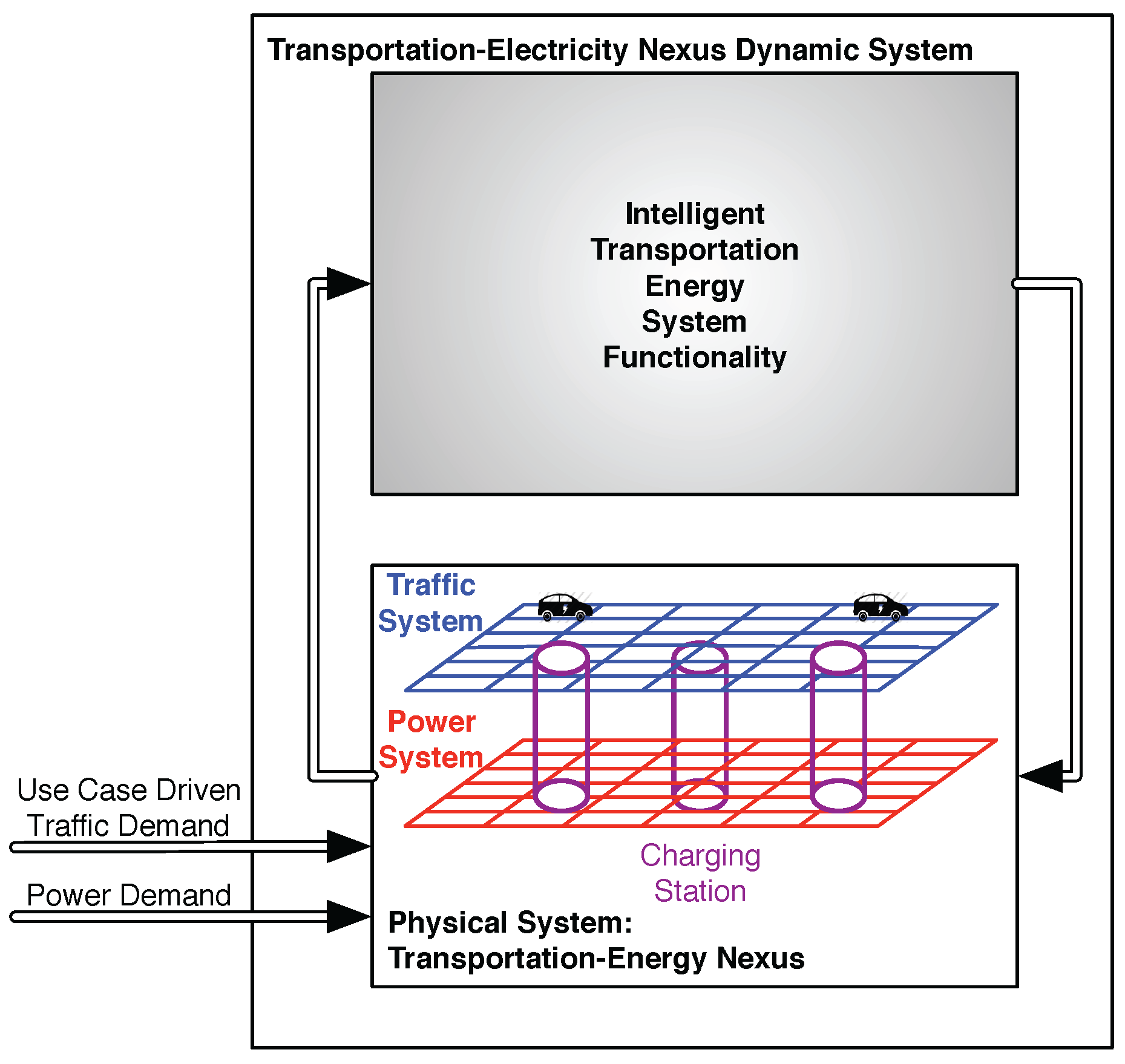
Figure 2.
The Symmetrica TEN topology: a test case for transportation electrification sesearch [98]: (a) on left, the transportation system topology; (b) on right, the electric power system topology.
Figure 2.
The Symmetrica TEN topology: a test case for transportation electrification sesearch [98]: (a) on left, the transportation system topology; (b) on right, the electric power system topology.
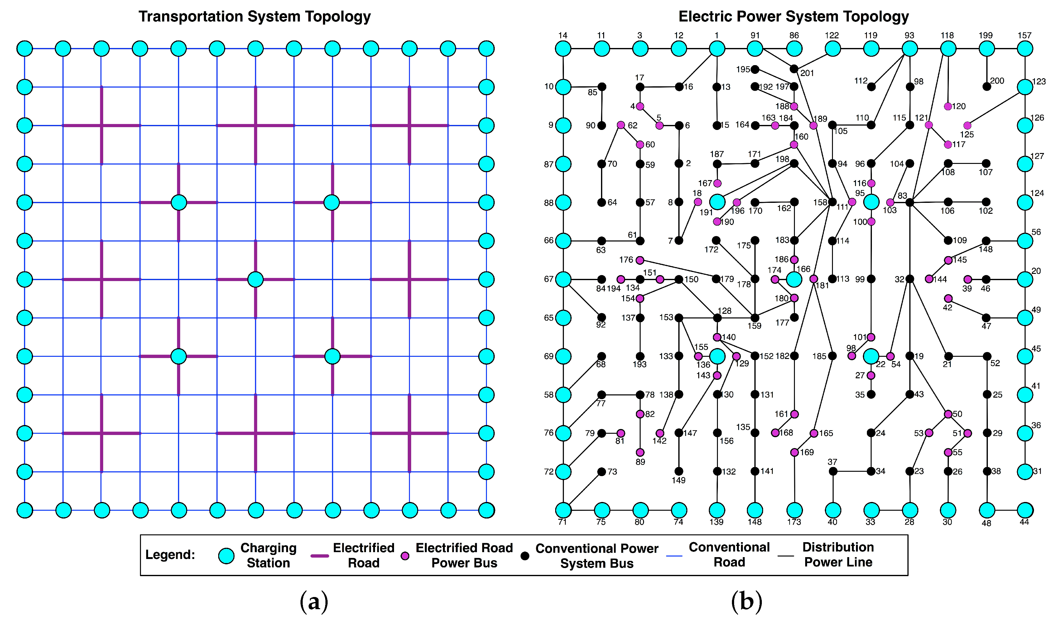
Figure 3.
Construction of part of the Symmetrica knowledge base from UML-notated classes for unique nodes and edges (charging station nodes and electric roads).
Figure 3.
Construction of part of the Symmetrica knowledge base from UML-notated classes for unique nodes and edges (charging station nodes and electric roads).

Figure 4.
A small subsection from the Symmetrica transportation topology is taken, and illustrated into a Petri-net. The Petri-net tracks the movement of three unique cars, represented by three colored tokens, through the network.
Figure 4.
A small subsection from the Symmetrica transportation topology is taken, and illustrated into a Petri-net. The Petri-net tracks the movement of three unique cars, represented by three colored tokens, through the network.

Figure 5.
Contrasting electric vehicle (EV) use cases: private car and taxi [76].
Figure 5.
Contrasting electric vehicle (EV) use cases: private car and taxi [76].
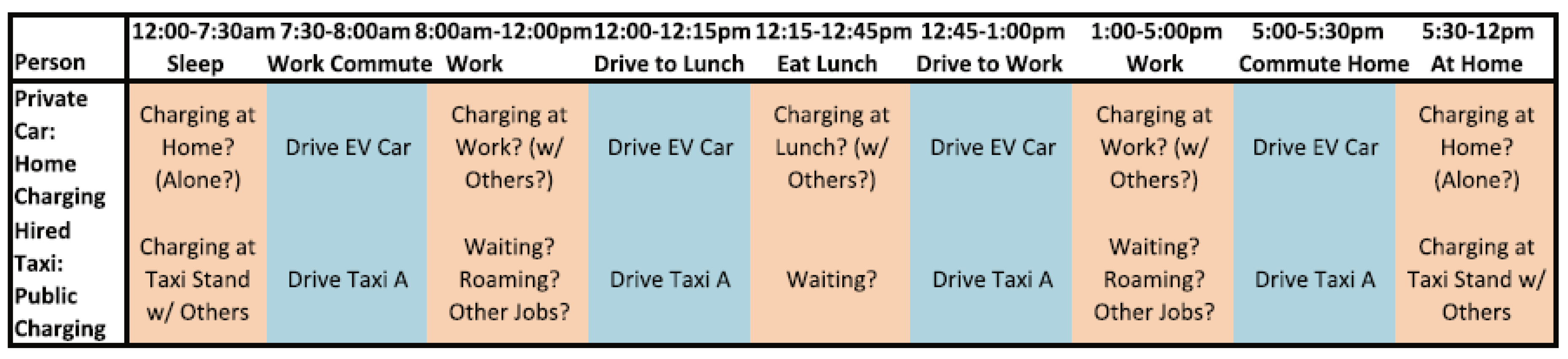
Figure 6.
Transportation Electrification Symmetrica test case results with 50% plug-in EV adoption. (a) Number of driving vehicles in time; (b) Number of parked vehicles in time; (c) Number of stationary charging vehicles in time; (d) Number of queued vehicles; (e) Active power through feeders (MW) in time; and (f) Bus voltages (p.u.) in time.
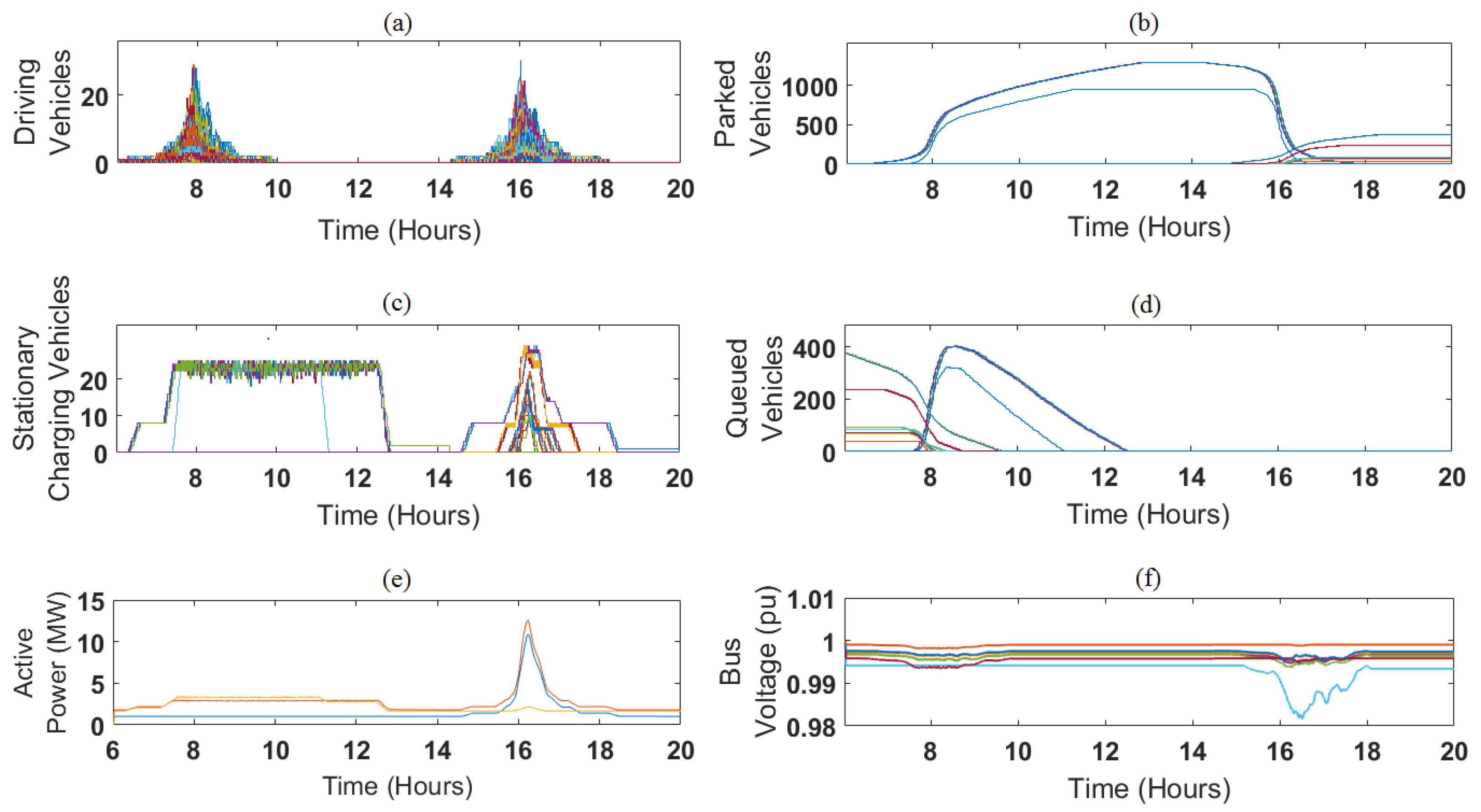

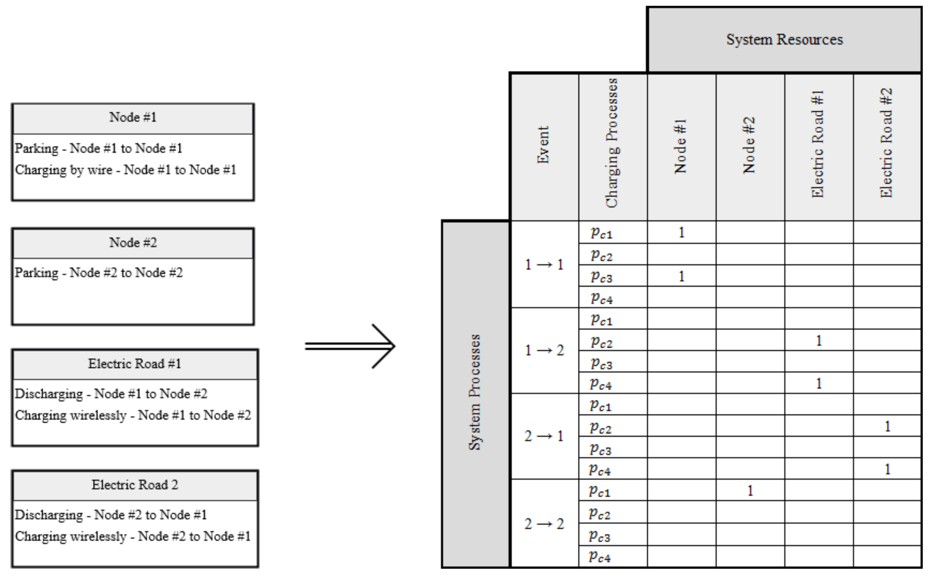
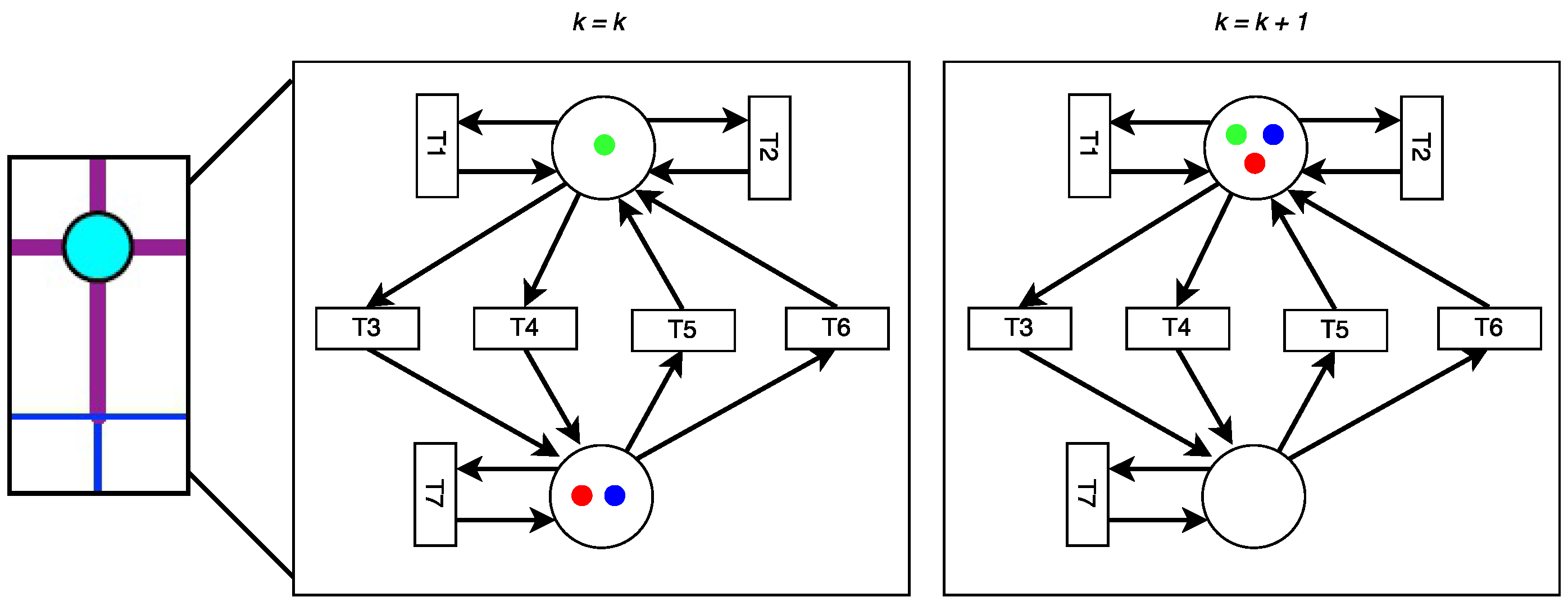
Table 1.
Intelligent transportation-energy system (ITES) operations decisions in the transportation-electricity nexus (TEN) [50].
Table 1.
Intelligent transportation-energy system (ITES) operations decisions in the transportation-electricity nexus (TEN) [50].
|
| System | M | B | H | |||
|---|---|---|---|---|---|---|
| LFES | Transformation | Transportation | Holding | Transforming Resource | Independent Buffer | Transporting Resource |
| Transportation Systems | Entry & Exit | Transportation | Charging | Stations | Intersections | Roads & Lines |
| Power Grids | Generation & Consumption | Transmission | Voltage Level | Generators & Loads | Storage | Lines |
Table 3.
Performance results for Symmetrica in 50% plug-in EVs scenario.
| Scenario | Quality of Service | Average Resource Utilization | Average EV Fleet Utilization | Average EV Fleet Availability | Effective EV Fleet Utilization |
|---|---|---|---|---|---|
| 50% Plug-In EVs | 82.6% | 2.7% | 2.8% | 86.0% | 3.3% |
© 2017 by the authors. Licensee MDPI, Basel, Switzerland. This article is an open access article distributed under the terms and conditions of the Creative Commons Attribution (CC BY) license (http://creativecommons.org/licenses/by/4.0/).
Share and Cite
MDPI and ACS Style
Van der Wardt, T.J.T.; Farid, A.M. A Hybrid Dynamic System Assessment Methodology for Multi-Modal Transportation-Electrification. Energies 2017, 10, 653. https://doi.org/10.3390/en10050653
AMA Style
Van der Wardt TJT, Farid AM. A Hybrid Dynamic System Assessment Methodology for Multi-Modal Transportation-Electrification. Energies. 2017; 10(5):653. https://doi.org/10.3390/en10050653
Chicago/Turabian StyleVan der Wardt, Thomas J.T., and Amro M. Farid. 2017. "A Hybrid Dynamic System Assessment Methodology for Multi-Modal Transportation-Electrification" Energies 10, no. 5: 653. https://doi.org/10.3390/en10050653
Note that from the first issue of 2016, this journal uses article numbers instead of page numbers. See further details here.