
Quantitative Evaluation of BIPV Visual Impact in Building Retrofits Using Saliency Models


Hochschule Luzern, Competence Centre Envelopes and Solar Energy, Technikumstrasse 21, Horw 6048, Switzerland
*
Author to whom correspondence should be addressed.
Energies 2017, 10(5), 668; https://doi.org/10.3390/en10050668
Submission received: 13 January 2017
/
Revised: 5 May 2017
/
Accepted: 8 May 2017
/
Published: 10 May 2017
(This article belongs to the Special Issue Solar Energy Application in Buildings)
Abstract
:BIPV (Building Integrated Photovoltaics) integration in urban spaces requires, not only careful technical, but also aesthetic considerations as its visual impact is seen as a kind of environmental effect. To manage this effect, different methods were developed to measure it; however, most existing evaluation methods are either based on subjective speculations and have no continuous criteria standards, or they do not show much relevance to neuropsychological findings. This paper presents an alternative and complementary method for evaluating the BIPV visual impact using the saliency method with an objective, quantitative and neuropsychological-based approach. The application of the method was tested and is discussed in the context of an example case study in Switzerland. Several different BIPV designs were developed for the case study, purposely in ways that made it difficult to rank their visual impacts with one’s subjective instinct. Using the proposed saliency method; however, the differences in BIPV visual impact across all designs could be identified, demonstrated and calculated sensitively. Potential applications of this proposed method include being a helping tool in deciding which BIPV design causes the least or most visual impact among others. Additionally, when combined with solar cadaster, the method enables a comprehensive estimation of BIPV potential in urban areas from both technical and societal aspects.
1. Introduction
1.1. The Rising Popularity of Photovoltaics (PV)
Driven by the improvements in manufacturing, price decrease and the raising awareness for a sustainable future, photovoltaics (PV) are becoming more popular worldwide, with the International Energy Agency (IEA) reporting a steady global growth in annual PV installations in the last few years [1]. The expansion of PV in Switzerland has taken place slowly, but fiercely. In 2009, the Swiss government decided that the electricity generated from BIPV (Building Integrated Photovoltaics) installations was to contribute 25% of the overall electricity production by 2030 [2]. Shaken by the nuclear disaster in Fukushima, Japan in 2011, the Swiss Federal Council, Parliament and Federal Office of Energy created the Energy Strategy 2050, which were strategies on how Switzerland should slowly grow independent of nuclear energy. Ambitious goals were set, such as an increase of energy efficiency, stabilization of electricity consumption, and an expansion of renewable energy [3]. Solar energy has become, among other renewable energies, the main alternative to nuclear energy and is expected to be an enormous development. The electricity production potential of PV in Switzerland is expected to reach up to 11.12 TWh/a by 2050 [4,5]. Analyses have also been made regarding the solar energy potential on building rooftops throughout Switzerland called the “solar cadaster” and it will be used as a promotion tool for solar energy usage targeted at private customers, and also as essential information for Swiss authorities when developing future planning strategies [6].
1.2. Restrictions for the Widespread Adoption of BIPV
With the growing number of BIPV being installed, people are realizing that, aside from its energy aspect, its visual aspect is a crucial element in deciding whether the BIPV can be installed. The main drive for this comes from heritage authorities, who claim that an abundance of PV will eventually harm the existing appearance of the city and buildings [7]. Additionally, the Swiss government also hopes to concentrate PV installation in urban areas, so that urban sprawl and damage to existing natural landscapes can be prevented. The urban planning law (RPG) Article 18a [8] states that “In building and landscape zones, solar installations on roofs that are considered as appropriately installed do not need to file for an installation application.” and that “Solar installations on cultural and natural heritages of cantonal or national importance always need to file for an installation application. They cannot affect these heritages obviously.” This ruling mainly encourages careful BIPV integration onto building envelopes and limits its visual impact.
Efforts to minimize BIPV visual impact can also be found at several other levels. Heritage protection authorities frequently express that they are open for discussions, urging for integration into planning teams in the early phase of building retrofit projects [9,10,11,12]. Responding to RPG Article 18a, the Swiss urban planning regulation (RPV) Article 32a [13] claims that if the following criteria are met, then the look of the BIPV on the roof can be considered as “appropriately installed”: (i) if the height of the BIPV does not exceed 20 cm above the roof surface; (ii) if the BIPV area does not exceed the roof plane; (iii) if the BIPV system is as low as possible in its reflectivity; and (iv) if the BIPV system’s area is compact. On the cantonal level, guidelines were published, explaining in the form of qualitative and formal design criteria on what the expected “appropriate looking” BIPV installations should be like [14,15,16,17,18]. For instance, it usually states that it is preferable to have a roof fully, rather than partially covered by the BIPV; or that it is desired that a BIPV glazing has a color resembling its environment, etc. The general attitude is that the lower the BIPV visual impact, the higher the fitness of its design.
Since the existing laws, regulations, and guidelines have not recommended specific measures to evaluate the BIPV visual impact, many academic researchers have developed evaluation methods to address this issue. The existing evaluation methods can be categorized either as qualitative or quantitative, depending on the criteria. The qualitative methods focus more on the aesthetic aspects of the BIPV system, for instance, it is proposed that having the module installed in a good position with appropriate dimensions, using pleasant surface texture and pattern will contribute positively to the integration quality of a BIPV design [19,20]. In other methods, a good BIPV integration requires the modules to be on the same planar surface as the building envelope, to respect the existing lines, or to form a regular and compact shape if visual attention is not desired, etc. [21,22]. Similar approaches can be found in References [23,24].
In the quantitative evaluation methods, one usually needs to decide the human field of view (the visual region that can be seen by the human observer) first. The perceived size of the BIPV system as a proportion of the field of view’s area is then proportional to the resulting BIPV visual impact [25,26]. In other similar approaches, the time factor is also considered: the perceived area is multiplied by the visual exposure time of the given PV for all viewers located in the surrounding. The visual exposure time of the static observers equals 12 h, which is the mean day-lighting hour per day throughout the year. For mobile observers (pedestrians and car drivers) moving on a certain road segment, the visual exposure time equals the time that they need to move from the start to the end of the road segment [27,28].
Generally, people expect that compliance with the required design criteria automatically leads to low visual impacts. The qualitative criteria generally originate from the empirical and instinctive design experiences of architects. In RPV regulations, cantonal guidelines, and qualitative academic evaluation methods, the resulting visual impact can only be estimated subjectively, so its strength remains immeasurable. Furthermore, the criteria standards are also strongly dependent on personal preferences. Regarding the quantitative evaluation methods, where the visible area is the way to measure the BIPV visual impact, the calculation process relies on pure geometric logic. Most importantly, most existing evaluation methods of BIPV visual impact lack a neuropsychological base. The relationship between the architectural context and the observer’s biological visual perception has not been considered. Due to these reasons, this paper intends to introduce an alternative and complementary evaluation method for BIPV visual impact, which is the saliency method, an objective, quantitative and neuropsychological-based approach.
2. Method
2.1. The Saliency Method
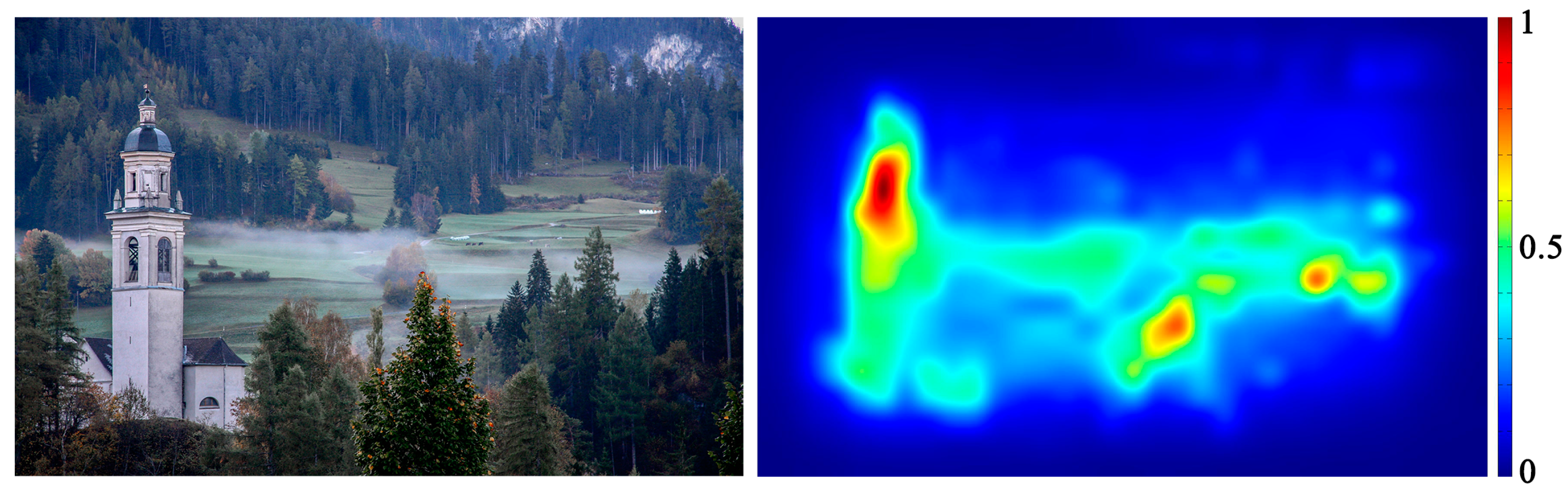
The proposed saliency method is largely based on the concept of the saliency model, a concept borrowed from the computer vision domain. It calculates the “visual saliency”, which means the probability of a particular image region attracting human visual attention in comparison to its surrounding. There are many different approaches to calculating visual saliency (for further detail, see Section 2.2). Usually, the contrast comparison mechanism of the human visual system is imitated by a saliency model, and a saliency map that predicts the visual saliency distribution of the corresponding visual scene is then produced (see Figure 1). On a scale from 0 to 1, a more conspicuous region will receive higher values in the saliency map, indicating that this region has a higher probability of being paid attention to by human eyes in this very visual scene.
Using a 2D rendering containing the BIPV system and the building of interest, the visual attention information of this visual scene can be analyzed and transformed into visual impact. It offers a quantified comparison between the visual impacts of different BIPV designs whose strengths are difficult to weigh qualitatively and instinctively. The principle and effectiveness of the saliency method have already been established in former works [30,31,32,33] and will be explained briefly in the following section. The workflow of the method is shown in Figure 2.
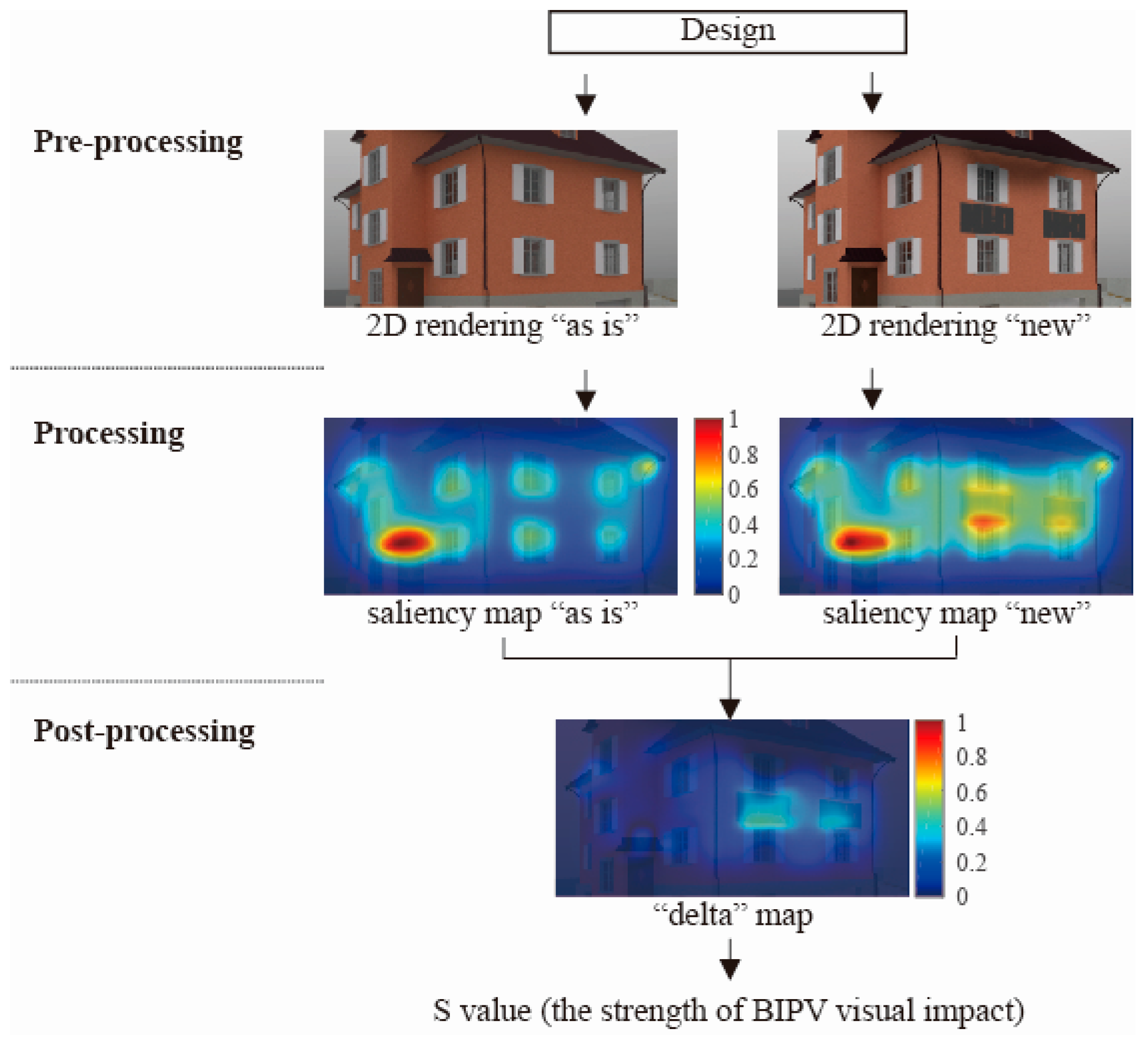
The methodology comprises 3 stages:
1. Pre-processing: Creating 2D renderings of the existing building with and without BIPV.
A 3D digital model that includes the most essential information of the building, such as its proportion, facade openings, colors and materials is created. Using this model with material and sky descriptions, 2D rendering “as is” is performed from the perspective that is most frequently seen by passing viewers. Next, a 2D “new” rendering is generated from the same viewpoint with the BIPV applied on the 3D model. Both renderings are produced using RADIANCE, a software that is capable of following the physical behavior of the light as closely as possible [34]. During this process, an overcast sky condition (CIE sky definition [35]) is used as it does not result in hard shadows, glaring sun reflections and exaggerated brightness in rendering images opposite to a clear sky condition.
2. Processing: Generating saliency maps for the 2D renderings.
The “as is” and “new” renderings are imported into the Matrix Laboratory (MATLAB) software. Using the given scripts, “as is” and “new” saliency maps are generated accordingly. All values on the saliency maps are automatically normalized to the range of 0–1. Saliency maps have the same pixel number as the renderings.
3. Post-processing: Analyzing the differences between saliency maps “as is” and “new.”
Given the identical perspectives, the difference between the saliency maps “as is” and “new” represents the variation of the visual attention in the renderings with and without the BIPV installation; and are calculated using the absolute difference between the saliency map “as is” and “new”:
Inspired by the Area Under Curve metrics [36,37,38], all pixels are sorted as either among the top 10% salient pixels or among the bottom 90% in the “delta” map. This can also be considered as the significance level of the distribution being set to 0.1 very roughly, to ensure that one does not miss detecting any difference that might exist. The strength of the difference between the saliency map “as is” and “new” is expressed by
The STt=10% is the threshold value between the top 10% of salient pixels and the bottom 90% of pixels, meaning that 10% of the pixels on the “delta” map have higher values than the STt=10%, and that 90% of the pixels on the “delta” map have lower values than STt=10%. S is the product between the STt=10% value and the maximum value on the “delta” map; they are multiplied by 100 for better expression. On a scale from 0–100, a low S value means either the vast majority of pixels have rather small values in the “delta” map, or/and that the maximum value in the “delta” map is low, meaning that the overall variation in visual attention in the visual image before and after the BIPV installation is small. A larger S value means either that most of the pixels are distributed within a value range with a larger upper bound, or that a particular region has especially high values in the “delta” map, so the overall change in visual attention is large. Thus, a smaller S value also means that with a lower visual impact, the building is more similar to its original state even after the BIPV installation.
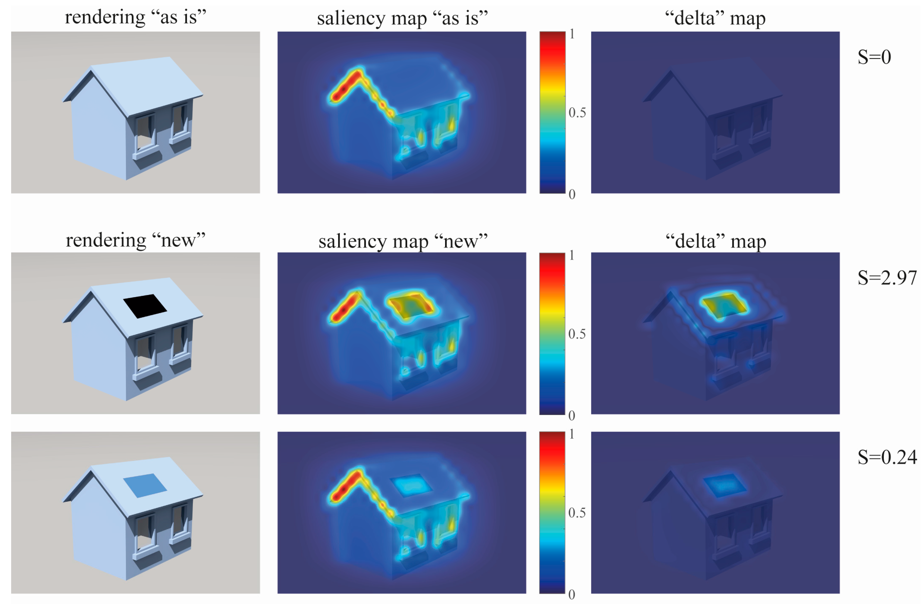
Using the color as a variable, Figure 3 shows an application example of the proposed saliency method. If a roof-integrated BIPV installation has a similar color as its surroundings, then its S value will be lower compared to a BIPV installation that has a color that is different from its surrounding.
However, it needs to be clarified that whether a particular BIPV design has a negative or positive influence on the existing building cannot be decided by the strength of the S value. The quality of the influence depends on the exact circumstance, e.g., as per the current accepted design value, the visual impact of a BIPV installed on downtown buildings should be as small as possible; while on an industrial building located in a suburban area, a higher BIPV visual impact is desired in order to draw visual attention. The proposed method merely offers the alternative to objectively quantify the BIPV visual impact that formerly mainly existed in a qualified form.
2.2. The Saliency Model
The approaches to calculate saliency maps are very different. The Itti–Koch–Niebur (IKN) saliency model was the very first saliency model to be based on psychological/neuropsychological findings [40]. Experiments have confirmed that human visual attention is guided by color, contrast sensitivity and orientation in the visual scene [41,42]. The IKN saliency model therefore first extracts information from the color, intensity, and orientation channels of the input image, then compares the contrasts within these separate channels using the center-surround operation. This operation roughly imitates how the human visual cell is capable of identifying the color or light contrast between its center and surrounding receptive fields [43]. Finally, the comparison results from these separate channels are normalized and combined into one final saliency map [29]. Similar neuropsychological inspired models also take the ability to spot the target between the distractors and motion detection ability of the human eyes into consideration [42,44,45].
Other saliency models are based on probability calculations, of which the Graph Based Visual Saliency (GBVS) model is an example. It also starts with extracting color, intensity and orientation information of the input image (although using other features is also possible) and compares the differences within these channels [39]. Each pixel is then be treated as a node in a directed graph that is compared with another node on the input image. The weight between the two nodes is proportional to their feature value difference and inversely proportional to their spatial distance. Finally, the nodes that are highly dissimilar to the surrounding nodes will have larger sums of weights and are therefore assigned higher saliency values. Even though the GBVS model is based on probability calculations, it is still inspired by human cognitive concepts. First, due to the nature of its algorithm, higher weights are assigned to the nodes located in the image center. This is desirable in the analysis as human eyes are more likely to focus on the image center. Second, it is believed that neurons in the human visual system can be seen as nodes. They connect with each other similarly as the nodes do, but through synaptic firings (instead of weighted edges in a directed graph) in deciding which area in the visual environment requires further processing.
Although numerous saliency models with other different approaches exist, it was decided to integrate the IKN and GBVS saliency models into the method proposed in this paper. The IKN is the first saliency model and often acts as the basis for the later ones. It has been shown to correlate with human eye movements in experiments where observers were asked to look freely at test images [46,47] and still remains an inspiration for many applications to this day [48,49,50]. The GBVS saliency model achieved good results in its accuracy according to the MIT saliency benchmark [51] and is especially suitable for predicting human visual attention when viewing landscape design photos [33]. The application of saliency models has proven to be quite helpful in several design sectors, such as advertising [52] and graphic design [53,54].
3. The Case Study
3.1. The Building and its BIPV Designs
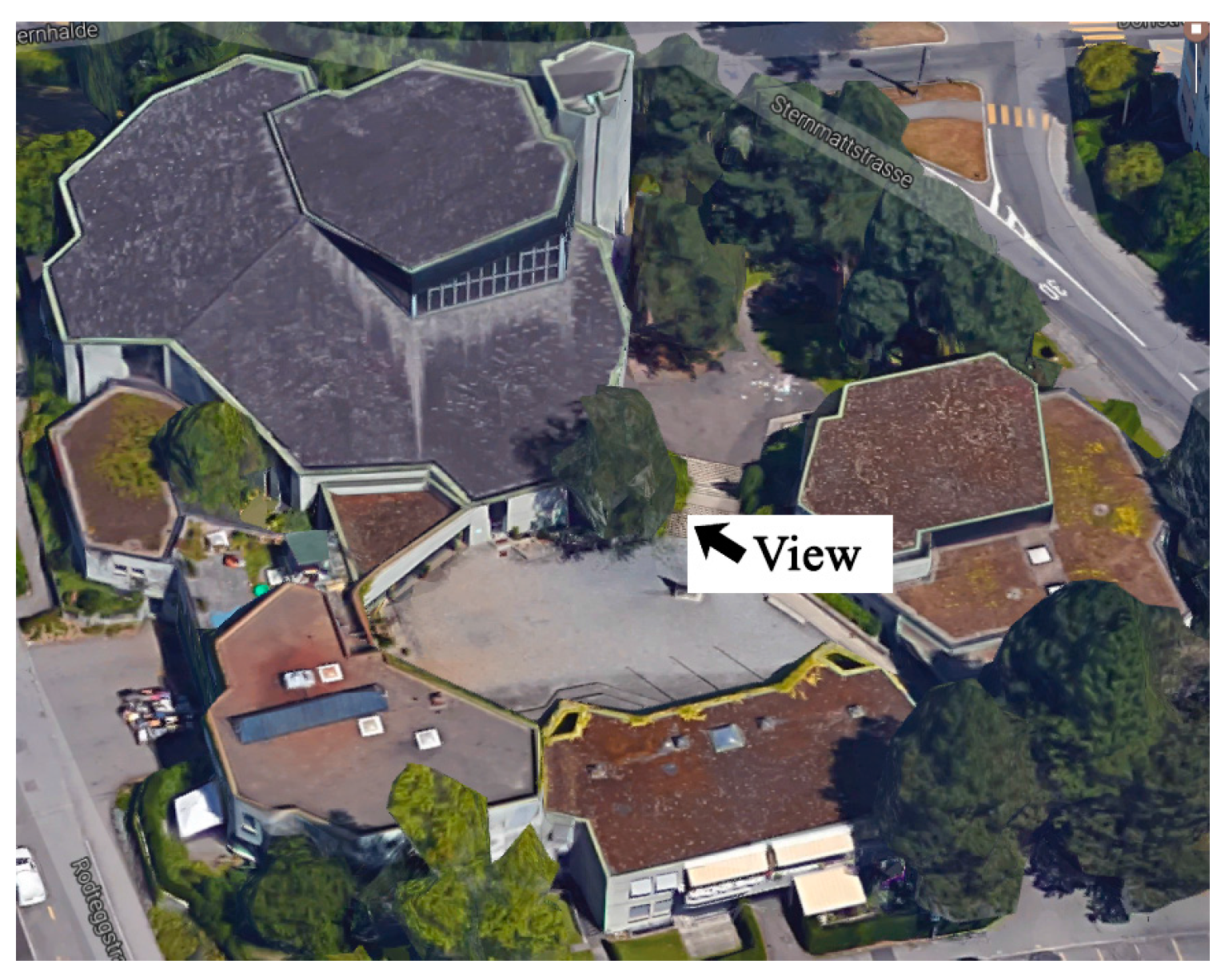
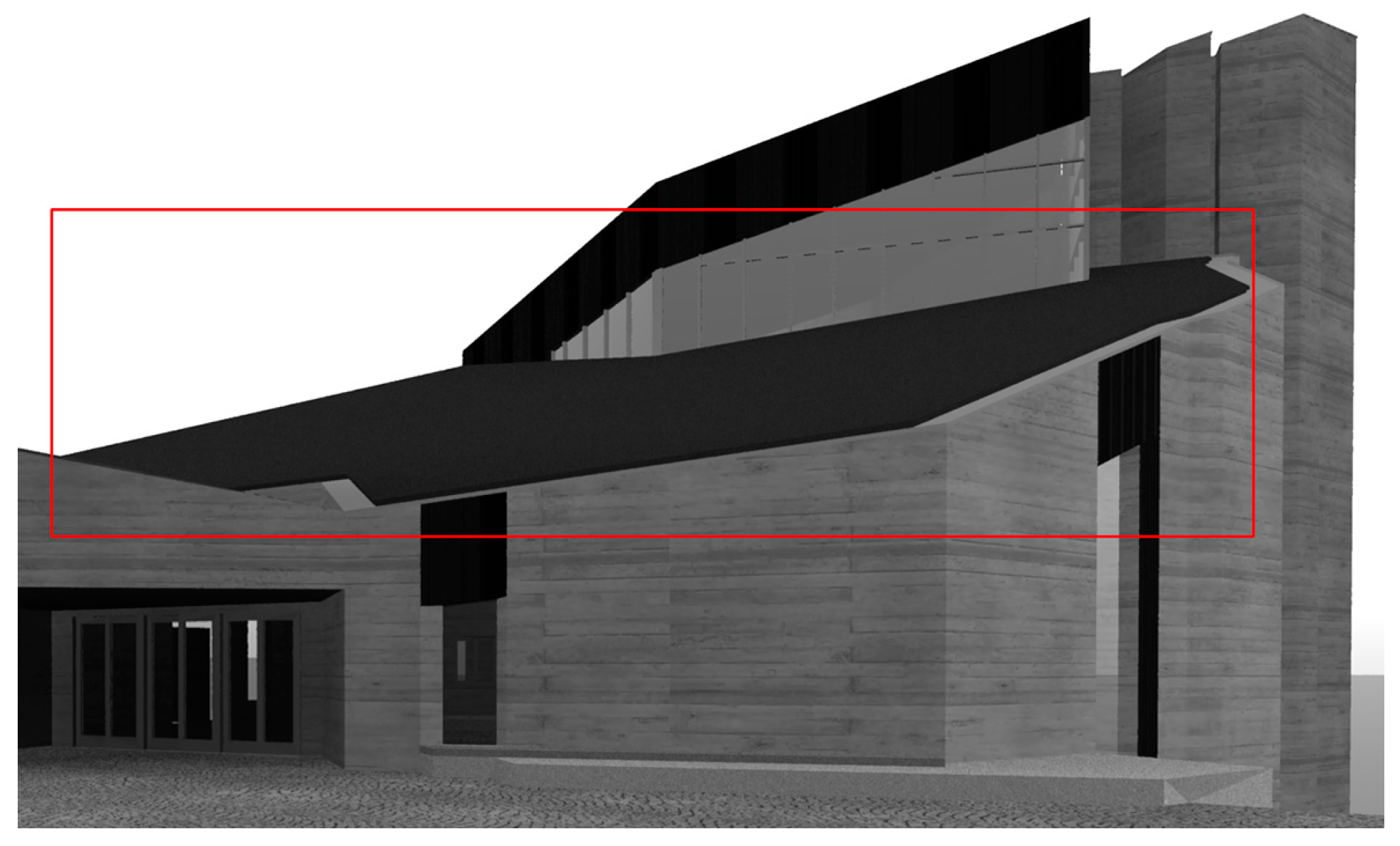
St. Michael, a church located in Lucerne, Switzerland, was used as the case study. The management team of the church hoped to integrate BIPV on its building envelope to demonstrate their support towards a greener future and to enhance the building’s energy efficiency. The most likely location for such an installation was the sloped roof of the church, as it faced south, had an optimal tilting angle and was covered in old roof tiles that had to be replaced. Other areas of the building envelope were to be left as is to preserve the appearance of the existing architecture. Three designs were proposed and presented to the management team and heritage departments of Lucerne (canton and city), so that they can choose one that they find most appropriate. The first design had a conceptual and bold approach, while the other two were more practical and cautious. As the building is in downtown Lucerne city, the BIPV visual impact was to be kept as low as possible. Figure 4, Figure 5 and Figure 6 show the church in its current situation, an aerial view of the church with the indication of the viewpoint for 2D rendering “as is”, and the rendering itself, respectively.
● Design 1—PVUp
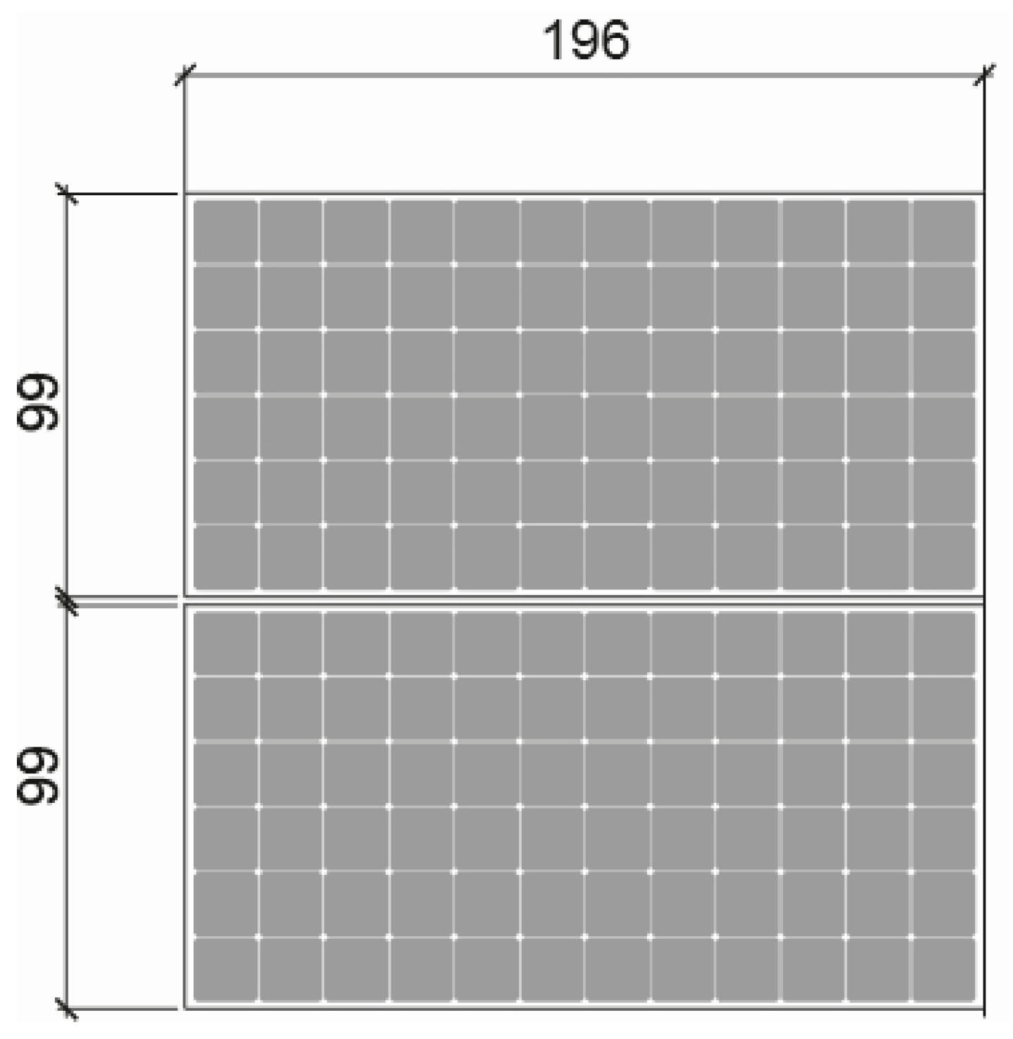
This design intended to apply the arranged BIPV arrays on the upper side of the sloped roof adjacent of the light tower. Standard BIPV modules, each with a size of 196 cm × 99 cm, were to be split into two rectangular groups and follow only the edges of the light tower (see the responding figure in Table 1). Figure 7 shows a partial layout plan of this design. This location is barely visible to the visitors due to its height, but can still achieve a demonstrative effect. This design also required less time and effort in installation and less technical equipment, e.g., cable connections. With the huge advantage in cost, the drawback of this design was that the outlines of the two PV groups did not exactly follow the profile of the church and was hence not ideal architecturally. In general, this design is a very simplified solution without much architectural concern.
● Design 2—PVBig
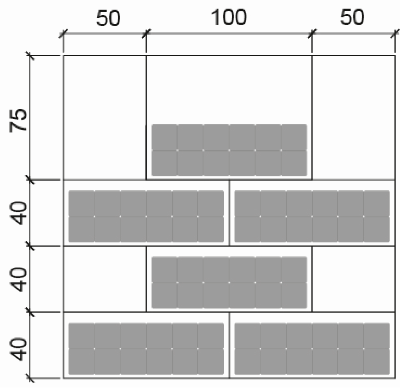
In Design 2, large BIPV modules covered the existing sloped roof of the church entirely (see the responding figure in Table 1). Dummy panels, which are tiles that look like PV modules but without the function to generate electricity, were used in places where a complete standard PV module could not fit. The PV modules were 75 cm × 100 cm, each covered by the modules above it by 35 cm (Figure 8). The visibility of the BIPV modules was high, but the tiled and homogenous pattern was expected to decrease their visual dominance. This design tried to preserve the original appearance of the existing church by arranging the BIPV in a similar pattern as before; however, the similarity was not as ideal as the third design PVSmall due to the use of large PV modules. No new silhouettes were introduced to the existing ones, so all the existing lines in the architectural context were respected.
● Design 3—PVSmall
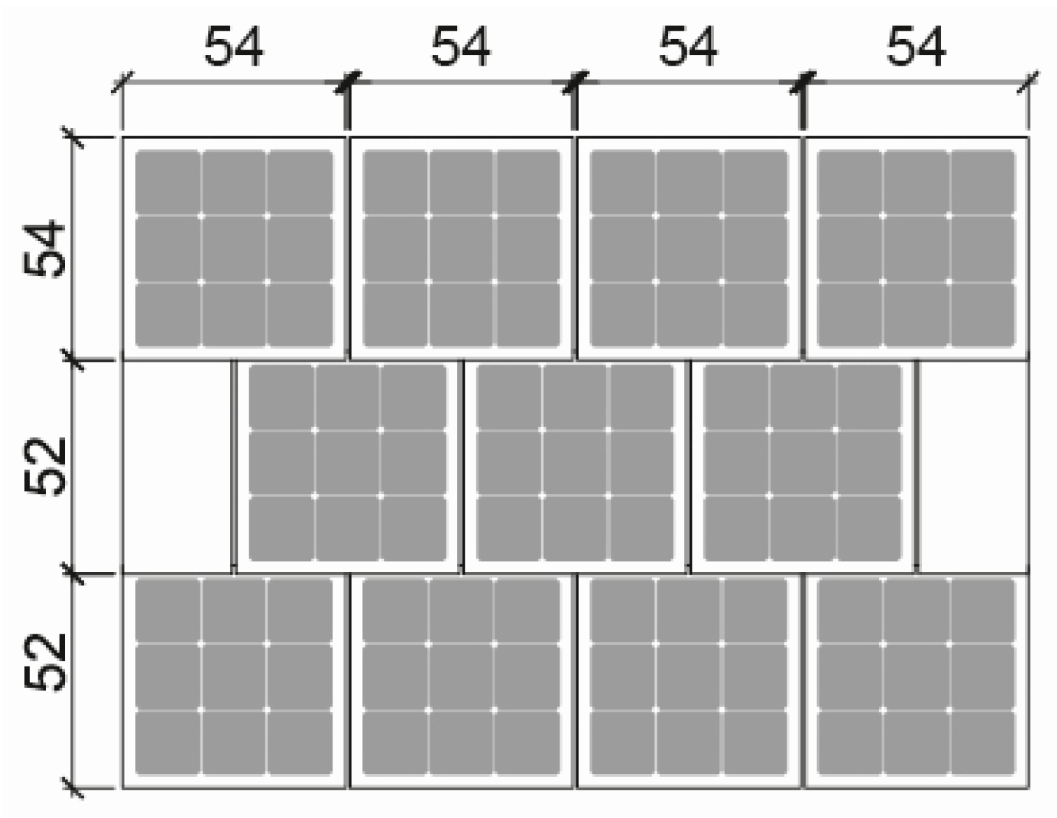
The third design was an improved variant of the design PVBig (see the responding figure in Table 1). Instead of standard PV modules, custom-made small modules of size 54 cm × 54 cm were used in this version (see Figure 9). This design was architecturally sensitive, as the smaller BIPV modules more closely resembled the existing roof tiles and their patterns than the large standard modules. Utmost respect was paid to the architectural appearance of the existing church complex with no strange lines introduced to disturb the present silhouettes. As with the PVBig design, the BIPV modules were also very visually accessible for visitors from almost all viewpoints, but still managed to be subtle by imitating the existing look of the roof tiles. However, the drawbacks to such a cautious and careful design approach include the fact that it would only be achieved through heavy planning work, high costs, and complicated technical requirements, e.g., an abundance of electric cables and extensive care.
3.2. Variation of BIPV Samples
The intention was to produce as much electricity as possible, as even with the high efficiency mono-crystalline BIPV modules, the annual heat demand of the church could only be partially covered when applying a heat pumper driven by the electricity generated with the BIPV (see Table 1). The monocrystalline module’s appearance was more homogeneous as the cells have a similar color to the backsheet. Polycrystalline modules have mostly blue cells, which result in a strong color shift between the cell and backsheet area. Although black polycrystalline PV cells do exist, they are not easy to find, and therefore not a very economical solution for the church. Furthermore, the thin film modules were not ideal for imitating the patterns of the roof tiles, as the combination of the small module area and low cell efficiency simply did not yield good results. Moreover, due to their production procedure, anti-glare glazing for thin film PV is not easily achieved, and high reflectivity is not desired for BIPV integration in urban spaces.
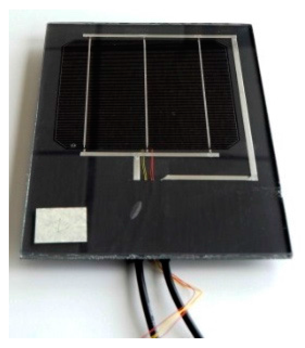
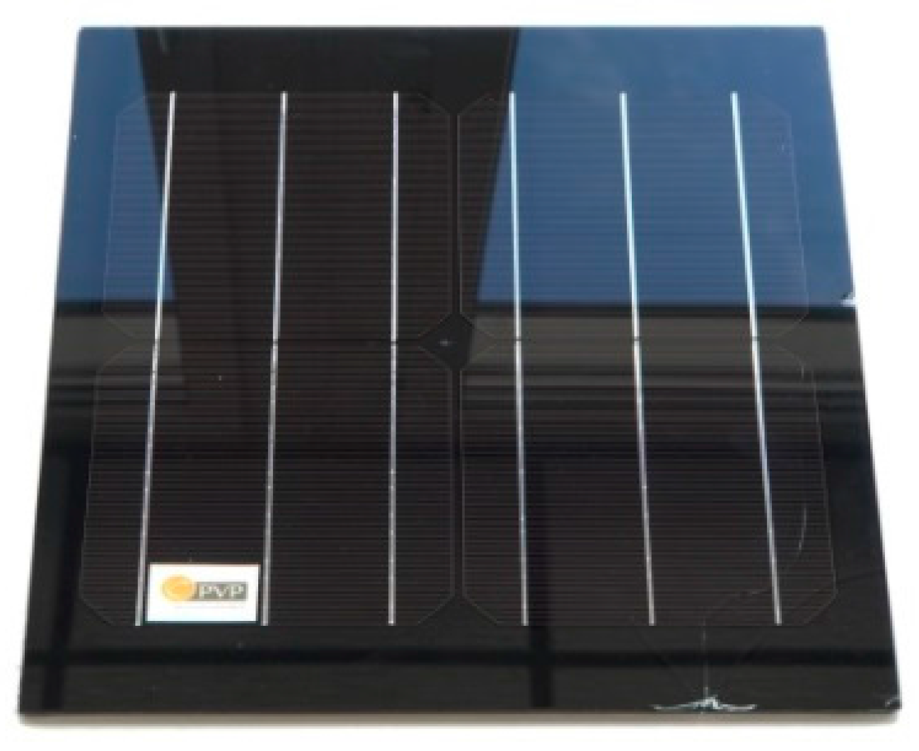
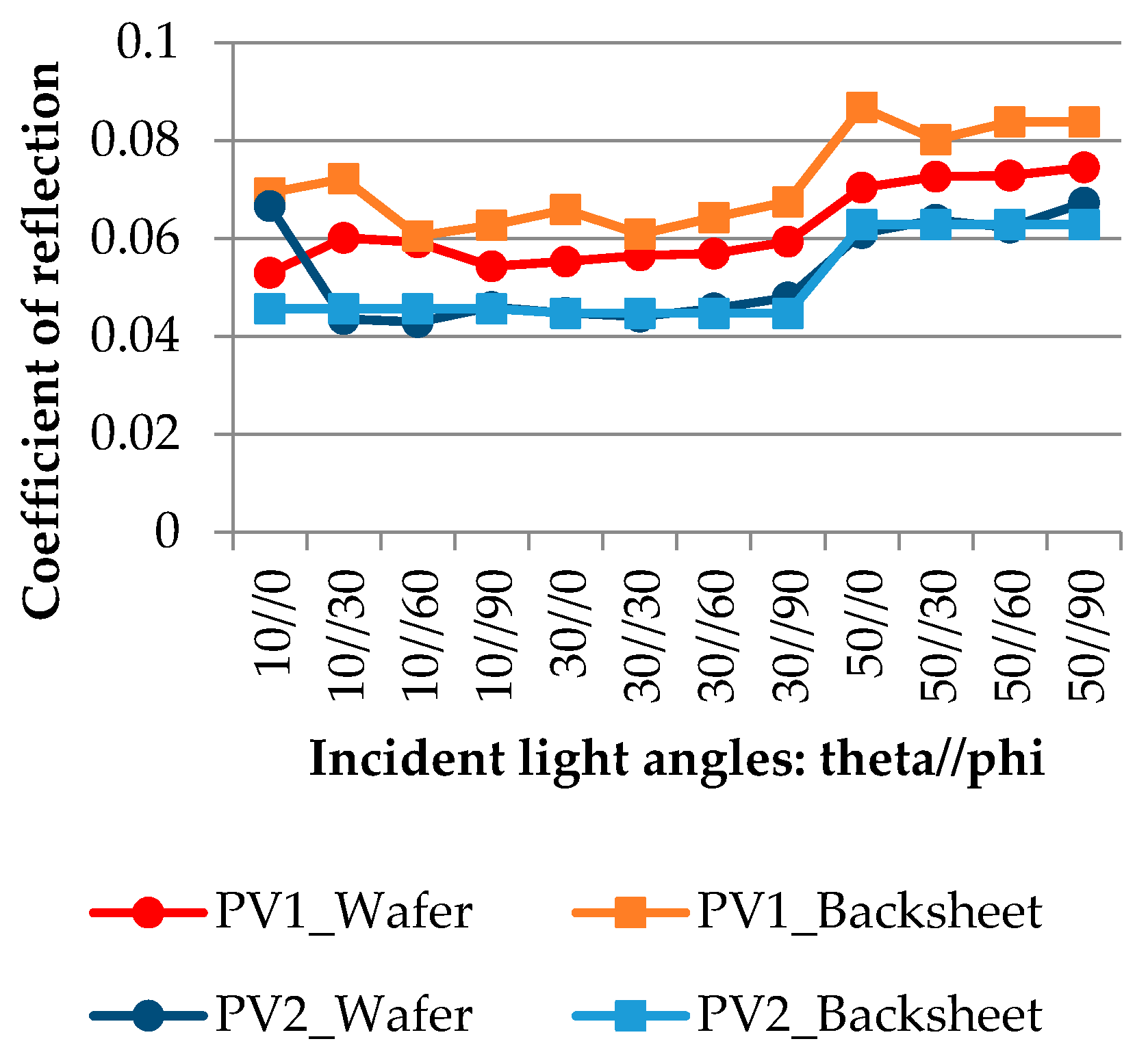
The reflection property of two typical mono-crystalline BIPV modules was measured and applied to the 3D digital models of the designs to ensure that realistic RADIANCE renderings could be generated to study how color, homogeneity, and reflectivity affected the BIPV visual impact. PV Sample 1 (Figure 10) is a custom-made, single mono-crystalline cell module with regular glass used as front glazing. The backsheet area color is dark grey and slightly lighter than the black wafer area. PV Sample 2 (Figure 11) is a module with four mono-crystalline cells. The black color of the backsheet area is quite similar to that of the wafer area. For both PV samples, two typical testing points were chosen: one in the backsheet and one in the wafer area, as they are the two kinds of areas on the PV module, resulting in four testing points in total. Figure 12 shows the reflection coefficients measured with a Goniophotometer. The results show that the reflection coefficient of PV Sample 1 was higher than that of PV Sample 2.
4. Results
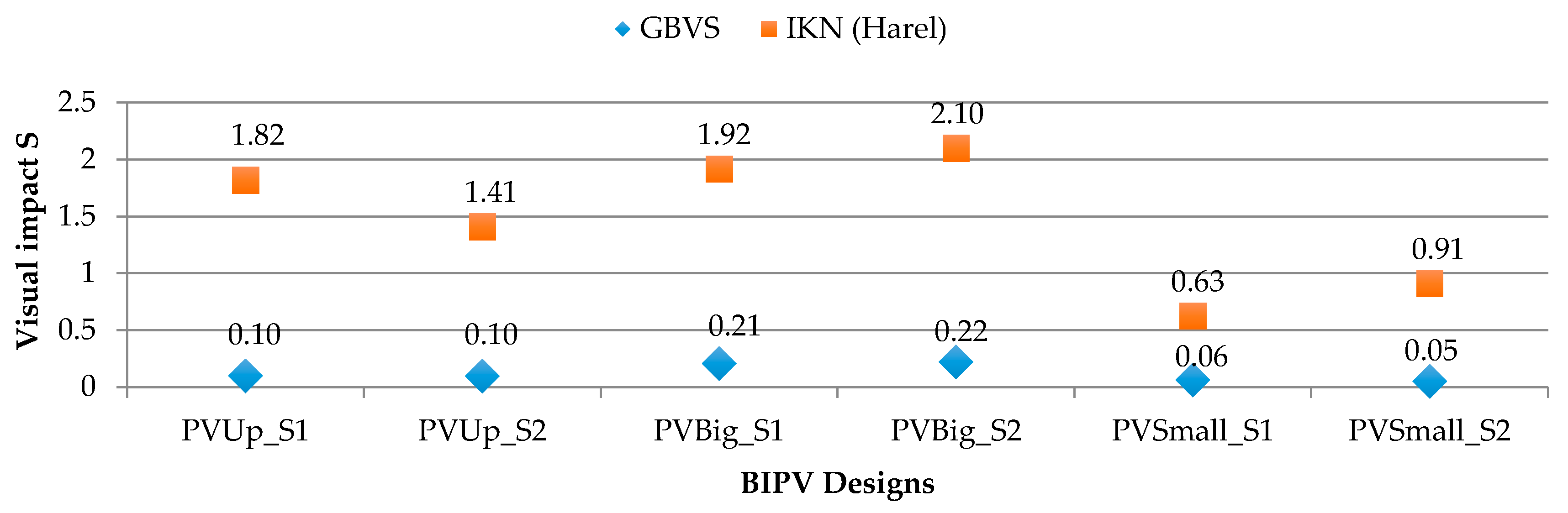
Figure 13 shows the “new” renderings of the designs using PV Sample 1. Figure 14 summarizes the BIPV visual impacts of the three different designs and their S values categorized by saliency models.
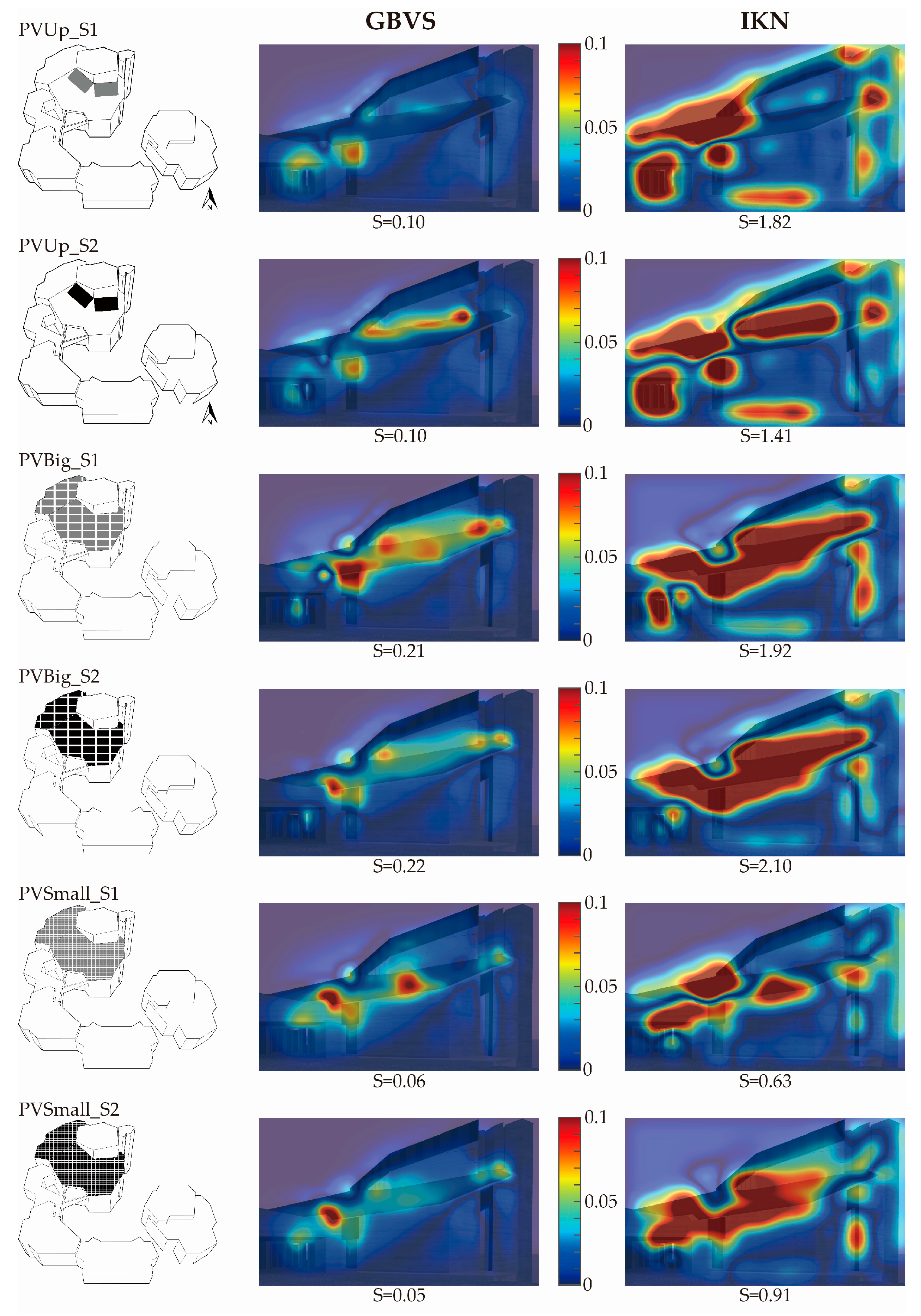
In both saliency models, the PVBig design had, against earlier subjective speculation, the highest visual impact (see Figure 14). Despite the homogeneous look of the BIPV panels, the tilting angle and orientation resulted in a larger color change in the roof area compared to the existing situation. This situation was not improved even when the more homogenous looking and less reflective PV Sample 2 was used. The resulting color made the roof resemble the opaque part of the light tower, thus weakening its saliency values and forced the visual attention that originally belonged to the roof to shift to the lower front window and the entrance door in the left of the image (see the “delta” maps in the third and fourth row in Figure 15).
Both saliency models GBVS and IKN showed that the visual impact of PVUp design was higher than that of the PVSmall (see Figure 14). The low S values of PVUp (compared to that of PVBig designs) could be traced back to the small visible area of the modules. A corresponding rendering (first row, Figure 13) showed that when installed very high up on the roof, only a little of the BIPV could be seen from an observer from the selected viewpoint. As per the GBVS saliency model, PVUp_S1 and PVUp_S2 had identical S values. Calculations from the IKN(Harel) saliency model showed that in the PVUp design, switching from PV Sample 1 to the less reflective PV Sample 2 resulted in a decrease of the S value.
The results produced from both saliency models showed that the PVSmall design had the lowest S values (see Figure 14). The tilting angle of the BIPV in PVSmall, in addition to the reflectivity, made the upper module side appear not entirely black, but rather greyish, like the existing roof tiles. The pattern formation from small custom-made BIPV panels also made the entire roof appear more monotonous. In the GBVS analysis, the visual impact of PVSmall_S1 was higher than that of PVSmall_S2. The IKN(Harel) saliency model, however, predicted that the visual impact of PVSmall_S1 was lower than that of PVSmall_S2. One possible reason is that when using PV Sample 2, the color of the roof would be darker, which meant that the contrast between the roof and its surrounding would be larger. It was also noted that there was a change in the dark red areas presented in the right last two rows of the IKN(Harel) “delta” maps in Figure 15, and it can be deduced that, according to the proposed saliency method, a higher reflective BIPV glazing would not necessarily result in a higher visual impact.
5. Discussion
The following reflections were made on the proposed evaluation method to guarantee more holistic analysis results in the future.
First, the visual analysis in this paper was made using only one single perspective and under only the overcast sky condition. The use of other perspectives and CIE sky conditions is necessary for making the analysis comprehensive, because it is highly likely that the S results depend strongly on the simulation conditions. A preliminary concept looks like this: one first needs to identify which perspectives are more prominent among an infinite number of others. Such screening tools have already been developed and widely used in terrain analysis [27,28,55,56]. From each of these prominent perspectives, an S value is calculated, which also has a weight attached to it that depends on the prominence of the corresponding perspective. The S value from the same perspective will also be produced twice, the first time under the CIE overcast sky condition, and then again under the CIE clear sky with sun condition. The first sky condition causes the least shadow in the “new” rendering, resulting in the smallest possible S value (S1); and the second sky condition will cause the largest possible S value (S2) due to the harsh shadows and potential glare in the “new” rendering. An S value calculated with any other CIE sky condition will fall between the range of S1 and S2. For each of these prominent perspective, its combined visual impact S value is then the average value between S1 and S2. In the final step, the overall S value for the BIPV design will be produced by dividing the sum of the combined S values by the total number of the prominent perspectives.
Second, the visual impact results were generated using the IKN and GBVS saliency models with two very different approaches. The differences in S values that are significant to the human eye are still unknown and needs to be verified. In the future, the reliable statistical evidence could be found using the following approach: By providing the “as is” rendering and several “new” renderings that belong to different ranges of S value, human test observers are asked to qualitatively evaluate the amount of deviance between the “as is” and “new” renderings. This result will be used as qualitative data. At the same time, the observers will also be wearing eyetrackers to record their eye fixation time lengths on each location of the renderings. The time length of the eye fixation on the BIPV installation is very likely to be proportional with the time they need to identify the deviance, and to be inversely proportional to the amount of deviance. In other words, the smaller the deviance between the “as is” and “new” renderings, the longer the observer needs to discover it. The time length record will be used as quantitative data and will complement the qualitative data. Together they will contribute to a more comprehensive understanding of the significance between the different S values.
6. Conclusions
This paper proposed an alternative and complementary method to evaluate the BIPV visual impact. To manage the visual impact that comes from the rising number of BIPV installations, first, one needs to be able to measure it properly. However, the current qualitative evaluation methods have difficulties in maintaining objectivity and their criteria standards are strongly dependent on personal preferences; and the existing quantitative evaluation methods do not usually have strong links with the known neuropsychological findings. Since the application of saliency maps is already found in various design areas and such maps provide reliable help in visual attention analysis, our proposed method intends to overcome the observed insufficiencies in the current methods by integrating the saliency model into its evaluation procedure. The authors hereby suggest an objective, quantified and neuropsychological-based approach to evaluate BIPV visual impact.
In the case study, the BIPV designs were deliberately developed in a way that made it difficult to weigh their visual impacts qualitatively using one’s instinct. In these situations, the existing qualitative evaluation methods are usually not sensitive enough to determine the BIPV visual impact. The existing quantitative evaluation methods are not suitable either, as the overall design approach of the BIPV system, and not the visible area, is more decisive to its visual impact. Using the proposed saliency method, however, the differences of BIPV visual impact across all designs can be identified, demonstrated, and sensitively calculated.
On a lower level, the proposed saliency method can be used as an alternative or a complementary tool for the conventional qualitative evaluation methods, by providing a different perspective in this area. On a higher level, it can be used in the urban planning sector by setting BIPV visual impact thresholds for different building zones. If combined with the solar cadaster, it would then be possible to estimate the true and comprehensive capacity of BIPV installations from both hard, technical as well as soft, societal perspectives. The application of the proposed method is not limited to just BIPV design, but can be expanded to any architecture design area that involves visual change analysis. This is especially important in a time where new technologies are constantly emerging and affect our existing living environment.
Acknowledgments
This publication is a result of the National Research Program “Energy Turnaround” (NRP 70), financed by the Swiss National Science Foundation (SNF). The authors would like to thank SNF for the financial support of the project “Active Interfaces”.
Author Contributions
Ran Xu developed the saliency map method and performed the case study; Stephen Wittkopf supervised the work and improved it with his insights; Christian Roeske designed the layout of the BIPV designs for the church roof and calculated their energy efficiencies.
Conflicts of Interest
The authors declare no conflict of interest.
References
- RTS Coorporation (Japan); Masson, G.; Nowak, S.; International Energy Agency Photovoltaic Power Systems Programme (IEA PVPS); Brunisholz, M.; NET Ltd.; Orlandi, S.; Becquerel Institute. Trends 2015 in Photovoltaic Applications. Report IEA-PVPS T1-19. 2015. Available online: http://www.iea-pvps.org/ (accessed on 5 January 2017).
- CR Kommunikation AG (Bern) Neue Energie. Neue Chancen. In Neue Energie für die Schweiz; 2010; Available online: http://www.nwa-schweiz.ch/xs_daten/NWA_Schweiz/aktualitaeten/NEch1_Magazin_DE_RZ.pdf (accessed on 2 January 2017).
- Bundesamt für Energie (BFE). Energiestrategie 2050. 2016. Available online: http://www.bfe.admin.ch/energiestrategie2050/ (accessed on 2 January 2017).
- Der Schweizerische Bundesrat. Botschaft Zum Ersten Massnahmenpaket Der Energiestrategie 2050 und Zur Vorksinitiative “Für Den Geordneten Ausstieg aus Der Atomenergie (Atomausstiegsinitiative)”. 2013. Available online: https://www.admin.ch/opc/de/federal-gazette/2013/7561.pdf (accessed on 2 January 2017).
- Eidgenössisches Departement für Umwelt, Verkehr, Energie und Kommunikation (UVEK); Bundesamt für Energie (BFE). Energieperspektiven 2050—Zusammenfassung. 2013. Available online: http://www.bfe.admin.ch/themen/00526/00527/06431/index.html?lang=de (accessed on 2 January 2017).
- Klauser, D.; Eidgenössisches Department für Umwelt, Verkehr, Energie und Kommunikation (UVEK); Bundesamt für Energie (BFE). Solarpotentialanalyse für Sonnendach.ch—Schlussbericht. 2016. Available online: http://www.bfe.admin.ch/geoinformation/06409/index.html?lang=de (accessed on 5 January 2017).
- Schweizer Heimatschutz. Solaranlagen, Baudenkmäler und Ortsbildschutz—Positionspapier. 2009. Available online: http://www.heimatschutz.ch/uploads/media/Positionspapier_Solaranlagen.pdf (accessed on 2 January 2017).
- Der Schweizerische Bundesrat. Bundesgesetz über die Raumplannung (Raumplannungsgesetz, RPG). 2016. Available online: https://www.admin.ch/opc/de/classified-compilation/19790171/index.html (accessed on 2 January 2017).
- Denkmalpflege des Kantons Bern und des Kantons Zürich. Energie und Baudenkmal—Gebäudehülle. 2014. Available online: http://feb.sia.ch/de/node/117 (accessed on 2 January 2017).
- Denkmalpflege des Kantons Bern und des Kantons Zürich. Energie und Baudenkmal—Solarenergie. 2014. Available online: http://feb.sia.ch/de/node/117 (accessed on 2 January 2017).
- Eidgenössische Kommission für Denkmalpflege; Bundesamt für Energie (BFE). Energie und Baudenkmal. 2009. Available online: http://www.bfe.admin.ch/energie/00588/00589/00644/index.html?lang=de&msg-id=28129 (accessed on 5 January 2017).
- Bundesamt für Landestopografie; Bundesamt für Energie (BFE). Denkmal und Energie—Historische Bausubstanz und Zeitgemässer Energieverbrauch im Einklang. 2015. Available online: http://www.bfe.admin.ch/energie/00588/00589/00644/index.html?lang=de&msg-id=59669 (accessed on 2 January 2017).
- Der Schweizerische Bundesrat. Raumplannungsverordnung (RPV). 2016. Available online: https://www.admin.ch/opc/de/classified-compilation/20000959/index.html (accessed on 2 January 2017).
- Kanton Luzern; Umwelt- und Wirtschaftsdepartement. Richtlinien Solaranlagen. 2015. Available online: https://solar.lu.ch/richtlinie_solaranlagen (accessed on 5 January 2017).
- Regierungsrat des Kantons Bern. Richtlinien—Baubewilligungsfreie Anlagen zur Gewinnung Erneuerbarer Energien. 2015. Available online: https://www.bve.be.ch/bve/de/index/energie/energie/downloads_publikationen.html (accessed on 5 January 2017).
- Kanton Thurgau; Department für Bau und Umwelt; Departement für Inneres und Volkswirtschaft. Solaranlagen Richtig Gut. 2015. Available online: http://www.denkmalpflege.tg.ch/xml_17/internet/de/application/f10227.cfm (accessed on 2 January 2017).
- Kanton St. Gallen; Energiefachstelle (Baudepartement); Denkmalpflege (Department des Innern). Solaranlagen vom Guten zum Besten. 2015. Available online: http://www.umwelt.sg.ch/home/Themen/Energie/erneuerbare_energien/sonnenenergie/photovoltaik/ (accessed on 10 January 2017).
- Stadt Solothurn; Stadtbauamt (Abteilung Stadtplannung). Richtlinien Solaranlagen. 2015. Available online: https://secure.i-web.ch/gemweb/stadtsolothurn/de/politikverwaltung/verwaltung/publikationen/?pubid=80398&action=info&highlight=Richtlinien+Solaranlagen (accessed on 10 January 2017).
- Probst, M.M.; Roecker, C. Criteria for architectural integration of active solar systems IEA Task 41, Subtask A. Energy Procedia 2012, 30, 1195–1204. [Google Scholar] [CrossRef]
- Probst, M.M.C.; Roecker, C. Solar energy promotion and Urban context protection: LESO-QSV Tool (Quality-Site-Visibility). In Proceedings of the PLEA 2015, Bologna, Italy, 9–11 September 2015. [Google Scholar]
- Zanetti, I.; Nagel, K.; Chianese, D. Concepts for solar integration development of technical and architectural guidelines for solar system integration in historical buildings. In Proceedings of the 5th World Conference on Photovoltaic Energy Conversion, Valencia, Spain, 6–10 September 2010. [Google Scholar]
- Lopez, C.P.; Frontini, F.; Bonomo, P. PV and Façade Systems for the Building Skin. Analysis of Design Effectiveness and Technological Features. In Proceedings of the 29th European Photovoltaic Solar Energy Conference and Exhibition (EU PVSEC 2014), Amsterdam, The Netherlands, 22–25 September 2014. [Google Scholar]
- Frontini, F.; Manfren, M.; Tagliabue, L.C. A Case Study of Solar Technologies Adoption: Criteria for BIPV Integration in Sensitive Built Environment. Energy Procedia 2012, 30, 1006–1015. [Google Scholar] [CrossRef]
- Vassiliades, C.; Savvides, A.; Michael, A. Architectural Implications in the Building Integration of Photovoltaic and Solar Thermal systems—Introduction of a taxonomy and evaluation methodology. In Proceedings of the World SB 14, Barcelona, Spain, 28–30 October 2014. [Google Scholar]
- Xu, R.; Wittkopf, S. Visuelle Beurteilung der Solaren Architektur. In Proceedings of the Swissbau 2014, Basel, Switzerland, 20–24 January 2014. [Google Scholar]
- Minelli, A.; Marchesini, I.; Taylor, F.E.; De Rosa, P.; Casagrande, L.; Cenci, M. An open source GIS tool to quantify the visual impact of wind turbines and photovoltaic panels. Environ. Impact Assess. Rev. 2014, 49, 70–78. [Google Scholar] [CrossRef]
- Fernandez-Jimenez, L.A.; Mendoza-Villena, M. Site selection for new PV power plants based on their observability. Renew. Energy 2015, 78, 7–15. [Google Scholar] [CrossRef]
- Rodrigues, M.; Montañés, C.; Fueyo, N. A method for the assessment of the visual impact caused by the large-scale deployment of renewable-energy facilities. Environ. Impact Assess. Rev. 2010, 30, 240–246. [Google Scholar] [CrossRef]
- Itti, L.; Koch, C.; Niebur, E. A model of saliency-based visual attention for rapid scene analysis. IEEE Trans. Pattern Anal. Mach. Intell. 1998, 20, 1254–1259. [Google Scholar] [CrossRef]
- Xu, R.; Wittkopf, S. Visual assessment of BIPV retrofit design proposals for selected historical buildings using the saliency map method. J. Facade Des. Eng. 2014, 2, 235–254. [Google Scholar] [CrossRef]
- Xu, R.; Wittkopf, S. Visual impact thresholds of photovoltaics on retrofitted building façades in different building zones using the Saliency Map method. In Proceedings of the CISBAT 2015, Lausanne, Switzerland, 6–8 September 2015. [Google Scholar]
- Xu, R. Visual Impact Assessment of BIPV in Building Retrofits Using Saliency Models. Ph.D. Thesis, École Polytechnique Fédérale de Lausanne, Lausanne, Switzerland, 2016. [Google Scholar]
- Dupont, L.; Ooms, K.; Antrop, M.; Van Eetvelde, V. Comparing saliency maps and eye-tracking focus maps: The potential use in visual impact assessment based on landscape photographs. Landsc. Urban Plan. 2016, 148, 17–26. [Google Scholar] [CrossRef]
- Ward, G.; Shakespeare, R. Rendering with Radiance: The Art and Science of Lighting Visualization; Booksurge Llc: Charleston, SC, USA, 2007. [Google Scholar]
- International Commission on Illumination Spatial Distribution of Daylight; CIE Standard General Sky ISO 15469:2004 (E)/CIE S 011/E:2003; International Commission on Illumination: Vienna, Austria, 2003.
- Judd, T.; Durand, F.; Torralba, A. A benchmark of computational models of saliency to predict human fixations. MIT Computer Science and Artificial Intelligence Laboratory Technical Report. 2012. Available online: https://dspace.mit.edu/handle/1721.1/68590 (accessed on 5 January 2017).
- Borji, A.; Sihite, D.N.; Itti, L. Quantitative Analysis of Human-Model Agreement in Visual Saliency Modeling: A Comparative Study. IEEE Trans. Image Process. 2013, 22, 55–69. [Google Scholar] [CrossRef] [PubMed]
- Riche, N.; Duvinage, M.; Mancas, M.; Gosselin, B.; Dutoit, T. Saliency and Human Fixations: State-of-the-Art and Study of Comparison Metrics. In Proceedings of the IEEE International Conference on Computer Vision (ICCV), Sydney, Australia, 1–8 December 2013. [Google Scholar]
- Harel, J.; Koch, C.; Perona, P. Graph-based visual saliency. In Proceedings of the Annual Conference on Neural Information Processing Systems (NIPS), Vancouver, BC, Canada, 4–9 December 2006. [Google Scholar]
- Borji, A.; Itti, L. State-of-the-Art in Visual Attention Modeling. IEEE Trans. Pattern Anal. Mach. Intell. 2013, 35, 185–207. [Google Scholar] [CrossRef] [PubMed]
- Wolfe, J.M.; Horowitz, T.S. What attributes guide the deployment of visual attention and how do they do it? Nat. Rev. Neurosci. 2004, 5, 495–501. [Google Scholar] [CrossRef] [PubMed]
- Le Meur, O.; Le Callet, P.; Barba, D.; Thoreau, D. A coherent computational approach to model bottom-up visual attention. Sacred Archit. J. 2006, 28, 802–817. [Google Scholar] [CrossRef] [PubMed]
- Niebur, E.; Itti, L.; Koch, C. Controlling the Focus of Visual Selective Attention. In Models of Neural Networks IV: Early Vision and Attention; Hemmen, J.L., Cowan, J.D., Domany, E., Eds.; Springer: New York, NY, USA, 2012; Volume 4, pp. 247–276. [Google Scholar]
- Navalpakkam, V.; Itti, L. An Integrated Model of Top-Down and Bottom-Up Attention for Optimizing Detection Speed. In Proceedings of the 2006 IEEE Computer Society Conference on Computer Vision and Pattern Recognition (CVPR’06), New York, NY, USA, 17–22 June 2006; Volume 2, pp. 2049–2056. [Google Scholar]
- Marat, S.; Ho Phuoc, T.; Granjon, L.; Guyader, N.; Pellerin, D.; Guérin-Dugué, A. Modelling Spatio-Temporal Saliency to Predict Gaze Direction for Short Videos. Int. J. Comput. Vis. 2009, 82, 231–243. [Google Scholar] [CrossRef]
- Parkhurst, D.; Law, K.; Niebur, E. Modeling the role of salience in the allocation of overt visual attention. Vis. Res. 2002, 42, 107–123. [Google Scholar] [CrossRef]
- Itti, L. Quantifying the contribution of low-level saliency to human eye movements in dynamic scenes. Vis. Cognit. 2005, 12, 1093–1123. [Google Scholar] [CrossRef]
- Suh, B.; Ling, H.; Bederson, B.B.; Jacobs, D.W. Automatic thumbnail cropping and its effectiveness. In Proceedings of the 16th Annual ACM Symposium on User Interface Software and Technology (UIST), Vancouver, BC, Canada, 2–5 November 2003; pp. 95–104. [Google Scholar]
- Lee, C.H.; Varshney, A.; Jacobs, D. Mesh Saliency. In Proceedings of the ACM SIGGRAPH 2005 Courses, Los Angeles, CA, USA, 31 July–4 August 2005; Volume 24, pp. 659–666. [Google Scholar]
- Wang, Y.-S.; Tai, C.-L.; Sorkine, O.; Lee, T.-Y. Optimized scale-and-stretch for image resizing. ACM Trans. Graph. 2008, 27, 118. [Google Scholar] [CrossRef]
- Bylinskii, Z.; Judd, T.; Durand, F.D.; Oliva, A.; Torralba, A. MIT Saliency Benchmark. Available online: http://saliency.mit.edu (accessed on 7 December 2014).
- Wilson, R.T.; Baack, D.W.; Till, B.D. Creativity, attention and the memory for brands: An outdoor advertising field study. Int. J. Advert. 2015, 34, 232–261. [Google Scholar] [CrossRef]
- Koide, N.; Kubo, T.; Nishida, S.; Shibata, T.; Ikeda, K. Art Expertise Reduces Influence of Visual Salience on Fixation in Viewing Abstract-Paintings. PLoS ONE 2015, 10, e0117696. [Google Scholar] [CrossRef] [PubMed]
- Rosenholtz, R.; Dorai, A.; Freeman, R. Do predictions of visual perception aid design? ACM Trans. Appl. Percept. 2011, 8, 1–20. [Google Scholar] [CrossRef]
- Bartie, P.; Reitsma, F.; Kingham, S.; Mills, S. Advancing visibility modelling algorithms for urban environments. Comput. Environ. Urban Syst. 2010, 34, 518–531. [Google Scholar] [CrossRef]
- Wheatley, D. Cumulative Viewshed Analysis: A GIS-based method for investigating intervisibility, and its archaeological application. In Archaeology and GIS: A European Perspective; Lock, G., Stancic., G., Eds.; Routlege: London, UK, 1995; pp. 171–185. [Google Scholar]
Figure 1.
An input image (left) and its saliency map generated with the Itti–Koch–Niebur (IKN) saliency model [29] (right).
Figure 1.
An input image (left) and its saliency map generated with the Itti–Koch–Niebur (IKN) saliency model [29] (right).

Figure 2.
Overview of the workflow of the proposed saliency method. In this figure, the Graph Based Visual Saliency (GBVS) model [39] was used to generate the saliency maps “as is” and “new”.
Figure 2.
Overview of the workflow of the proposed saliency method. In this figure, the Graph Based Visual Saliency (GBVS) model [39] was used to generate the saliency maps “as is” and “new”.

Figure 3.
An abstract application demonstration of the proposed saliency method. It shows with the example of a simple house how the different colors of a roof-integrated BIPV installation will affect the final S value. In the first row, it can be seen that, when there is no change in this visual scene, the “delta” map is entirely deep blue and the resulting S value is 0, meaning there is no resulting visual impact. Then, it can be seen that a black patch on the roof (second row) is generating a higher S value than a blue patch (third row), because the black patch is more “salient” than the blue one. The Graph Based Visual Saliency (GBVS) model was used to generate the saliency maps “new” and the “delta” maps [39].

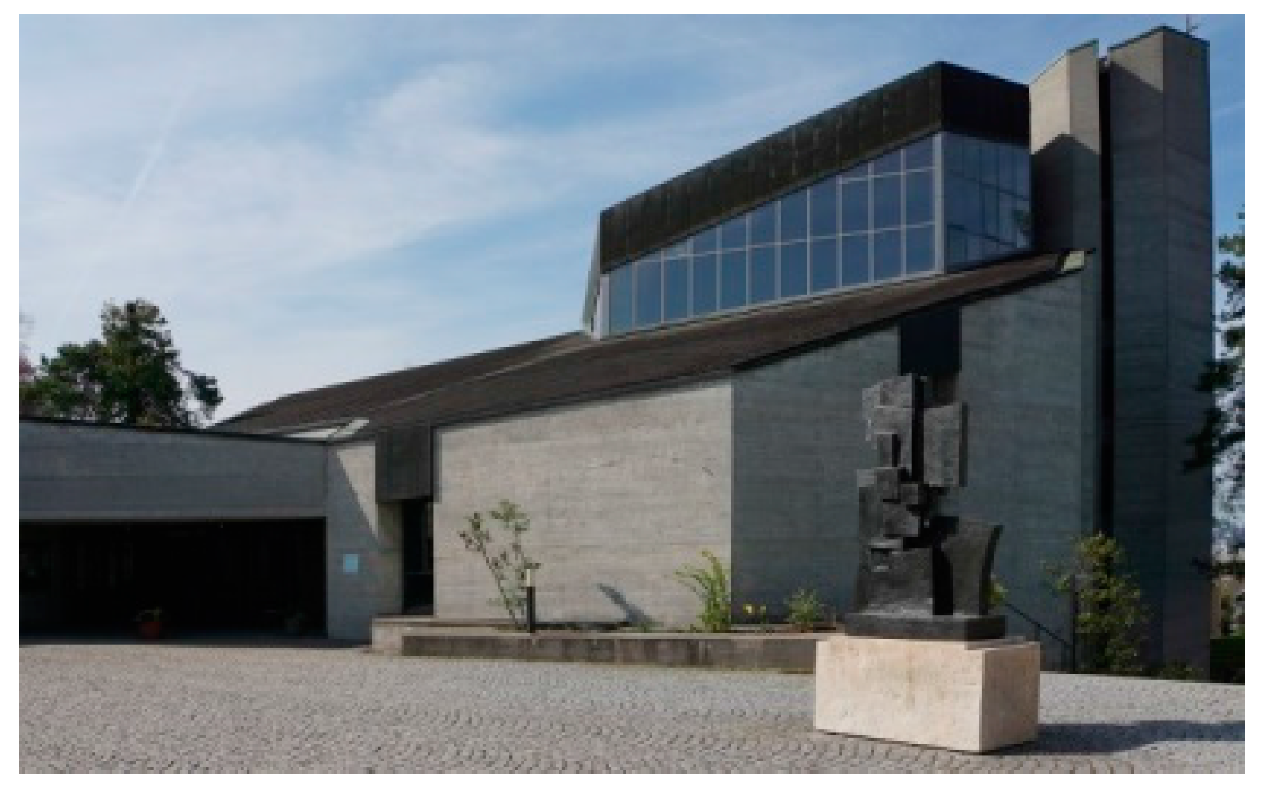
Figure 4.
The main church building. Photo taken in 2016.

Figure 5.
Aerial view of the church complex. (Image source: Google Maps. Imagery Date: 17 July 2014).
Figure 5.
Aerial view of the church complex. (Image source: Google Maps. Imagery Date: 17 July 2014).

Figure 6.
2D rendering “as is” produced with the RADIANCE software. The red box indicates the roof area where the roof tiles will be replaced by BIPV modules.
Figure 6.
2D rendering “as is” produced with the RADIANCE software. The red box indicates the roof area where the roof tiles will be replaced by BIPV modules.

Figure 7.
Partial layout plan of design PVUp.

Figure 8.
Partial layout plan of the design PVBig.

Figure 9.
Partial layout plan of the design PVSmall.

Figure 10.
PV Sample 1.

Figure 11.
PV Sample 2.

Figure 12.
The reflection coefficients of the measured PV materials.

Figure 13.
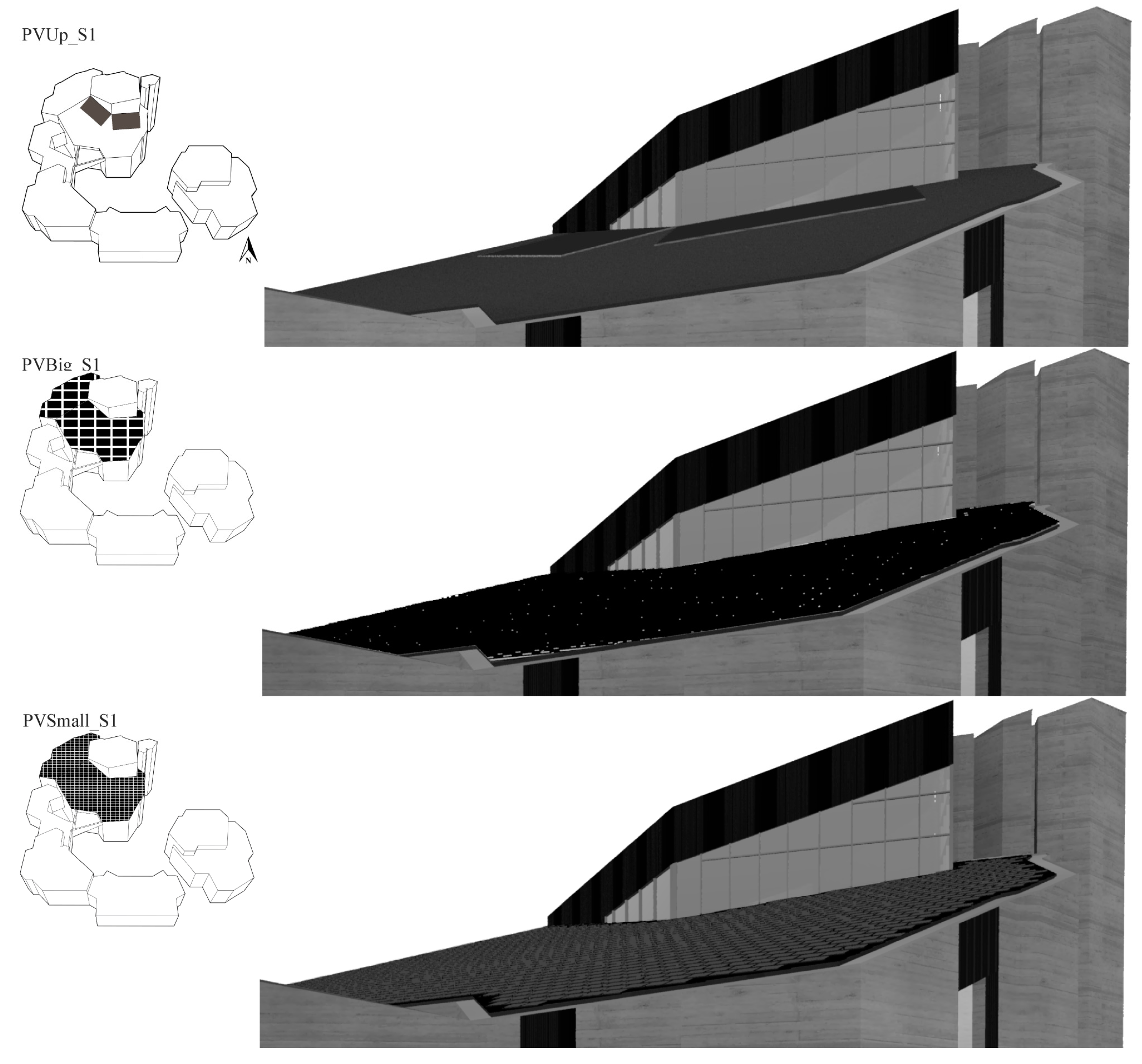
RADIANCE renderings of the designs. The pictograms in the left column show the location of the BIPV designs. The S1 in the names indicates that the rendering was made with material properties of PV Sample 1. The right column shows the repective renderings.
Figure 13.
RADIANCE renderings of the designs. The pictograms in the left column show the location of the BIPV designs. The S1 in the names indicates that the rendering was made with material properties of PV Sample 1. The right column shows the repective renderings.

Figure 14.
Visual impact S values of different BIPV designs as per the IKN and GBVS saliency models.
Figure 14.
Visual impact S values of different BIPV designs as per the IKN and GBVS saliency models.

Figure 15.
The “delta” maps and the S values of different BIPV designs. To demonstrate the results clearly, the value range on the color bar was set to 0–0.1.
Figure 15.
The “delta” maps and the S values of different BIPV designs. To demonstrate the results clearly, the value range on the color bar was set to 0–0.1.


Table 1.
General information about the different BIPV designs and how much of the church’s annual heat demand can be covered by the annual electricity production from the BIPV system. The black patches in each pictogram indicate the location of the BIPV system in each design.
Table 1.
General information about the different BIPV designs and how much of the church’s annual heat demand can be covered by the annual electricity production from the BIPV system. The black patches in each pictogram indicate the location of the BIPV system in each design.
| Design Name | PVUp | PVBig | PVSmall |
|---|---|---|---|
| Location of the PV System |  |  |  |
| Total BIPV area | 82.5 m2 | 336.9 m2 | 414.3 m2 |
| Nominal Power of the BIPV system | 13 kWp | 58.3 kWp | 53.8 kWp |
| Annual electricity production (under the condition that specific annual yield is 924 kWh/kWp) | 12 MWh | 53.9 MWh | 49.7 MWh |
| Annual heat production using a heat pump (with a coefficient of performance COP = 3) | 36 MWh | 161.7 MWh | 149.1 MWh |
| Coverage (in %) of the church’s annual heat demand (=397 MWh) | 9.0% | 40.7% | 37.6% |
© 2017 by the authors. Licensee MDPI, Basel, Switzerland. This article is an open access article distributed under the terms and conditions of the Creative Commons Attribution (CC BY) license (http://creativecommons.org/licenses/by/4.0/).
Share and Cite
MDPI and ACS Style
Xu, R.; Wittkopf, S.; Roeske, C. Quantitative Evaluation of BIPV Visual Impact in Building Retrofits Using Saliency Models. Energies 2017, 10, 668. https://doi.org/10.3390/en10050668
AMA Style
Xu R, Wittkopf S, Roeske C. Quantitative Evaluation of BIPV Visual Impact in Building Retrofits Using Saliency Models. Energies. 2017; 10(5):668. https://doi.org/10.3390/en10050668
Chicago/Turabian StyleXu, Ran, Stephen Wittkopf, and Christian Roeske. 2017. "Quantitative Evaluation of BIPV Visual Impact in Building Retrofits Using Saliency Models" Energies 10, no. 5: 668. https://doi.org/10.3390/en10050668
Note that from the first issue of 2016, this journal uses article numbers instead of page numbers. See further details here.