Abstract
Computational fluid dynamics is used to study the impact of the support structure of a tidal turbine on performance and the downstream wake characteristics. A high-fidelity computational model of a dual rotor, contra-rotating tidal turbine in a large channel domain is presented, with turbulence modelled using large eddy simulation. Actuator lines represent the turbine blades, permitting the analysis of transient flow features and turbine diagnostics. The following four cases are considered: the flow in an unexploited, empty channel; flow in a channel containing the rotors; flow in a channel containing the support structure; and flow in a channel with both rotors and support structure. The results indicate that the support structure contributes significantly to the behaviour of the turbine and to turbulence levels downstream, even when the rotors are upstream. This implies that inclusion of the turbine structure, or some parametrisation thereof, is a prerequisite for the realistic prediction of turbine performance and reliability, particularly for array layouts where wake effects become significant.
1. Introduction
The commercial exploitation of tidal energy on a large scale requires the deployment of arrays of full-scale tidal turbines. Given individual turbines of rated power of 1–2 MW, such arrays would have to consist of 50–100 turbines to approach the operating capacities of modern offshore wind farms. Individual turbines within a farm array will be affected by the wake of any turbines located upstream, and the large-scale environmental flow impact of the farm as a whole must also be understood; thus, modelling tidal arrays becomes a true multiscale problem. The application of computational fluid dynamics (CFD) can shed light in both areas, but this is extremely challenging from a computational perspective.
Wake effects in wind farms have been the subject of many studies. Models range from early empirical linear wake superposition approaches such as the Park model [1], through to Reynolds-averaged Navier–Stokes (RANS) CFD actuator disc models, large eddy simulation (LES) actuator disc [2,3,4] and actuator line models [5,6,7,8]. Porté-Agel et al. [9] simulated a wind farm using actuator disc and actuator line methods, the results comparing favourably with experimental data. Detailed reviews of wind turbine and wind farm wake modelling are given by Barthelmie et al. [10], Sanderse et al. [11] and Creech and Früh [12]. One striking feature of these models is that, barring a few exceptions [13,14], the turbine support structure is not modelled explicitly, and so, only the rotors affect the downwind flow. It is quite likely that, in the mid-to-far wake region, wake effects due to the structure are not important in wind farms; indeed, previous, validated studies of single wind turbines [15] and wind farms [4,16] have indicated that the tower and nacelle have negligible impact on the wake and consequently the performance of downwind turbines. The pertinent question here is, then, can the same be said for tidal turbines sited in swiftly flowing water, whose density is over 800 times that of air?
At the basin scale, it is common to use depth-integrated shallow flow models to assess tidal stream power. In many cases, depth-integrated models are used [17,18,19,20], with turbines represented by increased sea bed resistance, and the drag coefficient tuned to include both thrust and structural drag. These representations of turbines enable the thrust to vary with upstream flow speed, but are unable to resolve properly the three-dimensional flow kinematics that occur in the wake of a turbine rotor. Three-dimensional computational fluid dynamics (CFD) is capable of modelling resolved blade motion [21] in good agreement with laboratory experiments [22], but is expensive in terms of computational resources. In such models, simulating wakes over realistic distances downstream (i.e., many multiples of rotor diameter) is extremely challenging, especially with high-fidelity turbulence modelling techniques such as LES, due to the necessity of refining the mesh for the blade boundary layer. Therefore, parameterisation of the blades is required for simulations in larger domains. An early example comprised LES simulations of a turbine in 800 m-long tidal channel using a dynamic actuator disc turbine model [23]. This work found that the tidal turbine wake length, when scaled by power output, was on par with wind turbines. Others have focussed upon Reynolds-averaged Navier–Stokes (RANS) CFD models with actuator disc representations [24,25,26], obtaining good agreement with experimental data. Afgan et al. [27] and Ahmed et al. [28] compared blade-resolved RANS and LES simulations, demonstrating that LES predicts greater fluctuations in blade loads, whilst a similar work by McNaughton et al. [29] found that whilst LES produces better agreement with experiments, RANS models produce acceptable results for far less computational cost. Churchfield et al. [8] employed actuator line models to produce simulations of four turbines, without support structures, to examine wake effects on downstream turbines. See Section 6 for further discussion of these.
Using LES and the Fluidity CFD software from Imperial College London [30], we examine individual and cumulative contributions to the downstream wake of both the rotors and structure in a dual rotor, contra-rotating tidal turbine, located in a large rectilinear channel. The channel is sufficiently large to capture most of the wake, be of representative depth and contain realistic, fully-developed turbulent flow. Whilst computationally demanding, such simulations can provide a wealth of accurate detail, so giving insight into the complex interactions between the rotors and structure. This in turn can inform less expensive, quicker alternative models, such as those used in iterative design and assessment.
2. Initial Test Cases
For model verification purposes, two preliminary computational tests were conducted to ensure that the parameterisations gave realistic results in the absence of the turbine rotors. Simulations were of sheared flow in an empty channel, without, and then with, a vertical surface-piercing cylinder present. The configuration of the rotor and blades is dealt with separately in Section 3.
2.1. Basic Equations
For all simulations, an incompressible Newtonian fluid was assumed. A control-volume finite element discretisation [31] was used, with first-order, continuous velocity and pressure elements, and a Crank–Nicholson time stepping scheme. Large Eddy simulation (LES) modelled the effect of unresolved (subgrid) turbulence in fluid flows in the simulations. LES, first developed by Smagorinsky [32], was later adapted to channel flows by Deardroff [33]; the variant applied here within Fluidity takes into account mesh anisotropy [34], as Deardroff’s isotropic estimate for filter length breaks down as the cell aspect ratio increases [35]. Here, the filtered momentum and continuity equations are, respectively, in Einstein notation:
where is the filtered (above grid level) i-th velocity component, is the fluid density, p is pressure and is kinematic viscosity. For the following simulations, and . For application on anisotropic meshes, the subgrid eddy viscosity is represented by a tensor, defined as:
where is the Smagorinsky coefficient, set to 0.1 for all simulations [33], S is the rate-of-strain tensor and is the element size tensor. More details on the anisotropic LES formulation within Fluidity are found in Bentham [36] and Bull et al. [34].
Before running the ‘production run’ simulations, a series of test cases were run, and the results compared with published data. The results were used to validate the simulation configurations used, including mesh resolution, turbulence modelling and boundary conditions. For both cases, the inflow boundary conditions were identical.
2.2. Flow through an Empty Channel
2.2.1. Specification
Figure 1 shows the idealised channel domain, measuring 1 km × 200 m × 30 m. The chosen depth was close to that of Strangford Narrows where the SeaGen tidal device is situated [37], and the 1-km length allowed the wake behind the turbine to be captured within the model. Furthermore, the domain dimensions would allow large eddies tens of metres across to develop without impingement due to a restrictively small domain.
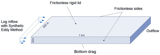
Figure 1.
The idealised tidal channel, showing boundary conditions and dimensions.
The surface of the channel was represented as a frictionless, rigid lid, and the lateral walls were also frictionless. Seabed drag was estimated empirically using the quadratic drag law with a bed friction coefficient of ; noting that the quadratic drag law has been found to fit measurements of turbulent tidal flow [38]. An open boundary condition was applied at the outflow. The synthetic eddy method (SEM) [39] was applied at the inlet to generate a turbulent inflow. The mean velocity profile was based on a logarithmic profile, i.e.,
where is the frictional velocity, K (=0.41) is the Von Kármán constant and is the roughness height of the channel bed, set to 0.05 m. B is a constant, which for turbulent open channels can be taken as [40].
If the flow speed at hub height is specified as , the frictional velocity can be calculated as:
where is the mean velocity at hub height, set to .
Building upon previous work [4], both the mean eddy length-scale and Reynolds stress profiles were specified as a function of height above the seabed for SEM, so that realistic turbulent inflow was generated. Eddy length-scales were taken from Milne et al. [41], whose measurements from the Sound of Islay agreed with Nezu and Nakagawa [40]. This gave the streamwise integral turbulence length-scales as:
Cross-stream and vertical components of eddy length-scale were specified as and respectively. The Reynolds stress profiles were taken from Stacey et al. [42], which following Nezu and Nakagawa [40] gives the three diagonal Reynolds stress components for unstratified channel flow as:
The normalised streamwise component, , is shown in Figure 2.
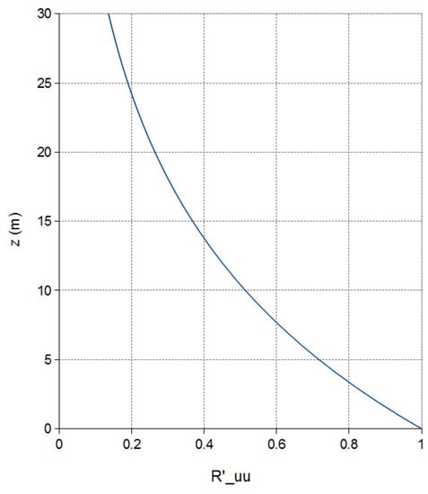
Figure 2.
Vertical profile of normalised streamwise Reynolds stress at the inlet, as a function of height.
For the computational mesh, the maximum element dimensions were [2 m, 2 m, 1 m], reduced to [1 m, 1 m, 0.5 m] within a distance of 2 m of the seabed. The overall mesh contained 17.6 million elements, partitioned across 480 computing cores. The time step was fixed at , with the pressure and velocity fields recorded every 1 s. The model ran initially for 30 min of simulation time to ‘spin up’, followed by another 30 min over which flow was to be recorded for analysis. At the time the simulations were carried out, high temporal resolution point probes (detectors) were not functional within Fluidity, which meant that full-domain data outputs were required. This in turn curtailed the sampling period, due to the excessive volume of data produced. Figure 3 shows a typical output of the velocity magnitude distribution throughout the channel at the end of the simulation (at time t = 1800 s). Roll-up of vortical structures can be seen at the bed, consistent with the development of turbulent eddies in open channel flow.
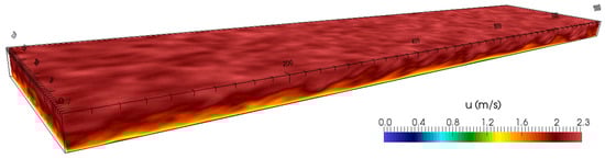
Figure 3.
Velocity magnitude distribution of the empty channel at t = 1800 s.
2.2.2. Results
Time-averaged vertical velocity magnitude profiles at a resolution of 0.5 m were taken from the centre of the channel, as shown in Figure 4a. These were calculated at different locations along the centreline of the channel; the distance downstream is plotted in units of D, the rotor diameter of the tidal turbine to be modelled (16 m), with the origin at 250 m downstream of inflow boundary. It can be seen that the time-averaged profile at is very similar to profiles further downstream, with no deviation at any point greater than at any height or distance downstream, even to .
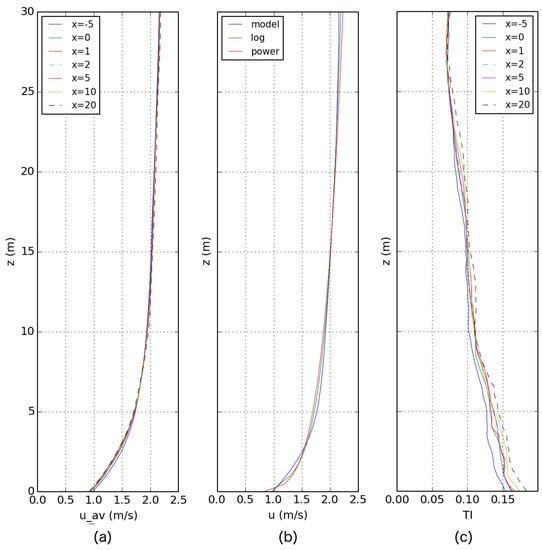
Figure 4.
Turbulent flow in an empty rectilinear channel, showing vertical profiles for (a) time-averaged velocity magnitude; (b) spatially-averaged velocity magnitude versus ideal log and power law profiles and (c) calculated turbulent intensity. Units for x are in D, the diameter of the turbine rotors (16 m). is where turbine rotors are to be placed, 250 m downstream of the inlet.
As a turbulent channel flow with bottom drag, a logarithmic vertical velocity profile should be expected. A logarithmic regression fit was applied to the mean of the velocity profiles in Figure 4a, which gave the following equation:
Nezu and Nakagawa [40] suggest that the logarithmic law may only be valid in the wall region and that a power law may be more appropriate. Therefore, a power law regression fit was also applied to the mean vertical velocity profile. As the roughness on the channel bottom is not explicitly resolved, the roughness height was instead derived from the skin friction coefficient [4] for a more appropriate fit. This gave the power law:
where .
If we express the exponent as , then Equation (11) gives . Whilst is a commonly-quoted figure [43], the derived value compares favourably with acoustic Doppler current profiler (ADCP) measurements from Strangford Narrows, from which on the flood tide and on the ebb tide [44]. Figure 4b superimposes both the log and power law fits on the spatially-averaged velocity magnitude profile. The model profile and the derived log-law match well, apart from a slight overshoot by the log-law near the surface and a slight undershoot near the channel bottom. This may be due to numerical diffusion arising from insufficient grid resolution. Unfortunately, increasing mesh resolution in this region is presently not an option owing to the prohibitively large computational expense; nonetheless, there is good overall agreement, particularly in the mid-region area of interest, near where the turbine rotors will be situated. To quantify the error between the model results and the log plot, the relative two-norm error was used:
where N is the number of sample points in the vertical profile, denotes the model results, and is the regression fit.
The error norms were determined as , or under 2% error, and , or just over 3% error. These were deemed acceptable margins. The turbulent intensity (TI) profiles in Figure 4c show as expected a low TI value (7%) at the surface, which gradually increases towards 15–18% at the channel bed. This compares well with Milne et al. [41], where ADCP measurements in the Sound of Islay gave a TI of 10–11% and a mean flow speed of , at 5 m above the seabed. The limited sampling frequency of 1 Hz mentioned in Section 2.2.1 means that the higher-frequency turbulence Nezu and Nakagawa [40] found in the lower section of the channel is not detectable. It is likely that if detectors had been available, a more pronounced peak near the bed would have appeared. Even so, the fit of the model data to the log and power law velocity profiles gives confidence that the channel simulation is a reasonable representation of turbulent channel flow.
2.3. Channel Domain with a Cylinder
The purpose of this test was to develop and validate an adequate representation of a structure within the domain, insofar as its effect on the flow is realistic. Flow past a cylinder represents an excellent test case for modelling the flow around a structure, as it is a widely-known problem [45,46,47,48,49] that has been studied extensively using CFD. It is well established that vortex shedding at the cylinder occurs at a predictable frequency for Reynolds numbers within the range ; this behaviour should be observed in the model.
2.3.1. Specification
Previous examples of simulated flow past a cylinder with LES have involved modelling the boundary layer equations [50,51], or using Van Driest damping functions to satisfy the zero eddy-viscosity condition at the cylinder surface [52]. Neither of these options was practical due to the size of the domain, and neither was available within Fluidity. Instead, an intermediate approach was adopted: to resolve the mesh finely around the cylinder and downstream as far as possible, but to also impose a quadratic drag boundary condition on the cylinder surface. Such a solution would be sensitive to both the mesh resolution near the cylinder and the skin friction coefficient chosen. To verify the approach, the Strouhal number St was calculated from the results:
where f is the frequency of the vortex shedding, is the diameter of the cylinder and is the upstream speed of the fluid. By examining the fluctuations in lift forces acting on the cylinder, the vortex shedding frequency f can be calculated and, so, the Strouhal number.
A vertical cylinder of a diameter of 3 m, similar to the main tower of SeaGen [53], was placed with its centre at [250 m, 100 m, 0 m] on the seabed, extending to the surface 30 m above. As confirmed by the empty channel tests in Section 2.2, this would allow the turbulence sufficient time to develop fully, whilst also avoiding any blockage effects due to narrowing of the passage between the cylinder and the channel walls. Mesh resolution was increased to [0.25 m, 0.25 m. 0.25 m] at the surface of the cylinder, as shown in Figure 5. The simulation ran for 1800 s, with a time step of . As with all of the simulations, the velocity and pressure fields were output every 1 s.
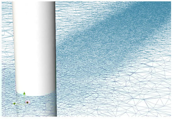
Figure 5.
Close up of a horizontal slice through the mesh at hub-height, showing the mesh resolution around and downstream of the cylinder. The resolution of the mesh at the cylinder’s surface is 0.25 m; this increases to approximately [2 m, 2 m, 1 m] over a distance of 10 m upstream, 20 m cross-stream and 250 m downstream.
2.3.2. Results
To determine the Strouhal number, the frequency of vortex detachment from the cylinder was checked by calculating the lift on a 1 m-thick ring on the cylinder at hub-height, i.e., . This was done for two reasons: firstly, as the cylinder is in vertically-sheared flow, the Reynolds number can be expected to vary widely from the top to bottom, and secondly, increased turbulence near the seabed would cause large pressure fluctuations not associated with vortex detachment, giving a noisier signal. The scale of the simulation can be seen in the instantaneous velocity slice in Figure 6, with a close up showing the vortex street caused by shedding in Figure 7.
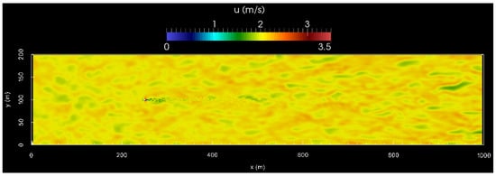
Figure 6.
Horizontal slice through the velocity field at z = 16 m and t = 900 s, showing the full extent of the wake behind the cylinder at the scale of the channel.
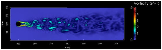
Figure 7.
Horizontal slice through the vorticity field at z = 16 m and t = 900 s, showing the vorticity generated by flow past the cylinder.
A fast-Fourier transform (FFT) was applied to the lift force fluctuations. The resulting power spectrum in Figure 8b contains a sharp peak around 0.22–0.225 Hz. For , Equation (13), this gives a Reynolds number of and a Strouhal number of = 0.3300–0.3375. Although this is above the values reported by Roshko [54] (St = 0.26–0.28) and Shih et al. [47] (St = 0.25), it falls within the lower limit of the measurements of Delany and Sorensen [45] who calculated St = 0.32–0.45, which is within the accepted range of Strouhal numbers given in the literature. The mean drag coefficient of the modelled cylinder was = 0.57, which compares favourably with experimental data for similar Reynolds numbers from Roshko [54] ( = 0.55–0.59) and Jones et al. [55] ( = 0.54). Although lower than Achenbach [56] ( = 0.6–0.7), in general, there is remarkably good agreement, given the very low blockage ratio presented here and the differences in oncoming flow profiles. Therefore, the combination of the cylinder surface mesh resolution and quadratic skin drag law was deemed sufficient for simulation of realistic wake effects.
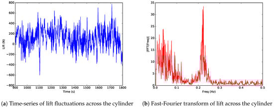
Figure 8.
The time-series of the lift force on the cylinder is shown in (a), with the FFT of lift in (b) showing a pronounced peak at about 0.22–0.225 Hz.
3. Turbine Formulation
The turbine model developed here builds upon previous work, where dynamic torque-controlled actuator discs with active-pitch correction were used to model wind turbines [15] and wind farms [4,16]. In the present model, actuator line techniques [5] have been used to represent the rotor, whereby the blades themselves are not resolved, but the forces exerted by them on the fluid are still present. In actuator line theory, the blade is replaced by the actuator line, and the forces are spread spatially via a normalised Gaussian distribution function to become body forces. In this implementation, we use a two-dimensional Gaussian distribution function, which is described below. The code for the model has been released as open-source, under the Lesser GNU Public License, Version 2.1 [57].
3.1. Methodology
The lift and drag force components per unit span acting on a blade are given by:
where and are the coefficients of lift and drag respectively, both functions of angle of attack and Reynolds number ; is the density of the fluid (for a tidal turbine, seawater) in which the blades move; is the relative speed of the fluid over the blades; and is the chord thickness as a function of r, the radial distance from the hub centre. In practice, is calculated for each cell point, using the local flow speed.
The Gaussian distribution functions at a point in space for turbine blade i of N blades in the rotor are expressed as:
where is a constant, the standard deviation that controls the filter width, and is the ring distance of point from the actuator line. was chosen with care, as too large a value could result in a heavily smeared solution, whereas too small necessitates an extremely fine mesh and very small time steps. In this case, it was found that one-twentieth of the rotor radius gave an acceptable trade-off between accuracy and computational effort.
Assuming that each blade has identical geometry, aerodynamic characteristics and blade pitch, then:
We apply this to determine the lift and drag terms as body forces, taking into account tip losses, to give:
where T is the Prandtl tip-loss factor [15,58]. As with previous work [4,15,23], blade-generated turbulence was then added via randomly fluctuating components. These body forces acting on the blades are translated into axial and azimuthal components; from Newton’s third law, the consequent body forces on the flow are equal and opposite. Each time-step, these terms are calculated and passed back to the CFD solver to be included in the Navier–Stokes momentum equations. The force terms above are also used to calculate the power output of the turbine. By first calculating the net torque acting on the fluid, we can then calculate the resistive torques turning the generator and blades [4,15], thus turning the drive shaft and the blades. Both the drive chain and the power conversion have associated energy losses, which are written as:
where is the actual power, is the ideal power without energy losses, is the drive train efficiency and the generator and power conversion efficiency. We used and , the values specified in Bedard [59] for the MCT/Siemens SeaGen device. An active pitching algorithm was used which maximises total lift, matching the behaviour of SeaGen [60]. Further details of the numerical model can be found in Creech et al. [4].
3.2. Parameterisation
The rotor configuration was based on that of Marine Current Turbines SeaGen device [61], i.e., dual rotors, aligned horizontally. As many of SeaGen’s technical details are commercially sensitive and not readily available, rotor and performance specifications were sourced from journal papers [53,59,61,62,63,64]. Details often disagreed between papers, so discretion was applied in deciding on the values listed in Table 1. To validate the chosen parameters, candidate models were tested against performance data from SeaGen, as shown in Figure 9.

Table 1.
General specifications for the modelled turbine.
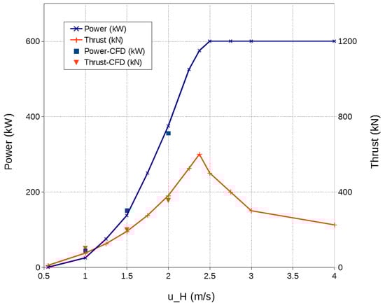
Figure 9.
Time-averaged power (blue) and thrust (red) for a single rotor of SeaGen, as a function of mean hub-height flow speed . The solid lines represent data sourced from Douglas et al. [63] and Fraenkel et al. [53,61]; the squares and triangles represent simulation results.
The aerofoil chosen was a NACA 63–415 type, which has desirable lift characteristics. The lift and drag at limited angles of attack were taken from previous work [4], which based its aerofoil data on that from the Airfoil Catalogue [65]. Blade geometry was completely unknown, so as a starting point, the equation for the predicted flow angle at a turbine rotor was taken from Burton et al. [58]:
where is the predicted inflow angle as a function of radial distance r, is the design tip-speed ratio and , where R is the radius of the turbine rotor. If the optimum angle of attack for a given blade , then the blade twist can be given as:
was calculated from the lift and drag coefficient charts for the chosen aerofoil type, as per Creech et al. [4]. This then provided the blade twist angles along the blade.
No information was available on chord thickness, so this was calculated using the equation for an ideal optimised blade derived from blade-element theory ([58], Chapter 3), i.e.,
where is the rotor solidity (N is the number of blades, c the local chord thickness), and is the lift coefficient at optimal operation, which is calculated from lift and drag performance data. Rearranging gives:
where is the right-hand side of (23). The chord length can now be defined as a function of r for a blade with specified characteristics.
3.3. Test Cases and Results
Test cases were devised to check that the specification of the rotor, the blades and the generator properly represented the real tidal turbine, in a channel flow . To lessen computational requirements, a single rotor would be tested in a simulation domain much smaller than the empty channel test case, measuring 250 m × 100 m × 30 m. No support structure was included to further reduce the number of elements required. The turbine rotor was positioned much closer to the inlet, at [50 m, 50 m, 16 m]. Such a short domain was acceptable because only the performance of the turbines was of interest, and the wake effects could be ignored. Mesh resolution was increased towards the rotor, so that the actuator volume contained approximately 19,000 points. In the final simulations, the turbine rotors would be operating at below the rated power, so only hub-height flow speeds below 2.5 would be tested. Three mean hub-height flow speeds were considered: .
Figure 9 compares the resulting mean power and thrust from each case with published performance data. The model yields slightly larger time-averaged values for power and thrust at when compared to the published data, but it is in good agreement for both power and thrust when is at 1.5 and 2 , to within a maximum relative error of 8.8%. The cause of the over-performance of the model at the lowest flow speed could be down to minor discrepancies in the rotor, blade or generator specifications, but this cannot be confirmed. Other possible causes may be rotor-rotor wake interaction in the dual rotor configuration; this will be examined in Section 4. Notwithstanding this, the results provide reasonable confidence in the modelled rotor performance at the target hub height flow speed of .
4. Full-Scale Turbine Simulations
4.1. Overview
The simulations were based on the tidal channel test case in Section 2.2, as it was sufficiently large (1 km × 200 m × 30 m) to allow realistic turbulence structures to develop and to capture the extents of the turbine and structure wakes. To isolate and analyse the contributions of the various components of the turbine to the downstream wake, three different scenarios were considered: (a) with dual contra-rotating rotors and no structure; (b) with the complete support structure only and (c) with both the rotors and the structure present. For each of these scenarios, the mean hub-height flow speed was set to , with turbulent inflow conditions provided via the synthetic eddy method used in Section 2.2.1. These simulations were run until the turbulent flow was fully developed and the statistical properties of the flow, such as turbulence intensity and time-averaged flow speeds, had become stable; this was a minimum of 2700 s in all runs. Each simulation was then run for a further 900 s, during which full sets of data for the velocity and pressure were saved to disc for analysis each second for post-processing. As detectors were not available, higher frequency sampling of velocity fields for spectral analysis was not possible.
Nevertheless, the 900-s sampling period was sufficient to provide time-averaged velocity profiles that appeared to be statistically stationary. All simulations were run on ARCHER, the U.K.’s national academic supercomputer, using 2400 computing cores each of which typically used 1.5 MAUs (million allocation units), with a wall time of 2–3 days.
4.2. Configurations
The support structure model is shown in Figure 10, which was based on SeaGen’s design. The model consists of a 30 m high, 3 m diameter monopile that pierces the water surface, with a crossbeam at a height of 15 m above the sea bed. The crossbeam is 27 m broad and 4 m long, encompassing the monopile, and contains angled sections on either side that rise 1 m and taper to 3 m long at their furthest extent. Solid nacelle sections measuring 1 m × 3 m × 2 m are located at the ends of the crossbeam. The crossbeam edges have been smoothed to have a curved surface of radius 0.5 m, as have the nacelles. This arrangement closely follows details given by Fraenkel [53], Neill et al. [64] and Fraenkel [61], whilst also taking cues from Keenan et al. [37]. The more complex quadropod base was not adopted in the final design, due to the prohibitive mesh refinement and complexity that would have been required. The structure was placed on the seabed in the empty rectilinear channel described in Section 2.2, such that the monopile base was centred at [250 m, 100 m, 0 m].
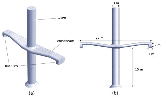
Figure 10.
The turbine structure: (a) a perspective view illustrating the main components and (b) a head-on view indicating important dimensions.
The contra-rotating rotors case used the design developed in Section 3.2. The rotors were positioned in front of the solid nacelle structures, with the first rotor T1 at [247 m, 87 m, 16 m] and the second rotor T2 at [247 m, 113 m, 16 m]. The blades were oriented on T1 and T2 so that the lift-induced torque would cause clockwise and anti-clockwise rotations, respectively, thus forming the contra-rotating pair shown in Figure 11. Each rotor was connected to a modelled generator, and like SeaGen, these generators operated asynchronously [66]. The mesh resolution was highest near the blades and reduced gradually with distance from the rotors, as can be seen in Figure 12.
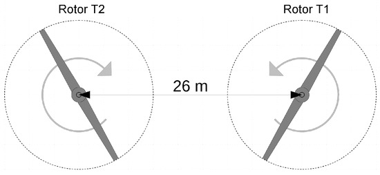
Figure 11.
Contra-rotating rotors with centres separated by 26 m.
Figure 12.
Horizontal slice at hub height through the mesh for the dual rotors only case. Mesh resolution increases sharply toward the rotors and reduces gradually downstream to the resolution used in the empty channel case.
The final case combined the dual rotors and structure configurations above. Table 2 lists the mesh resolutions and time-step sizes for each case.
Table 2.
Simulation configuration details.
5. Results
This section examines the time-averaged velocity and turbulence intensity data obtained from the full simulations of turbulent flow in the rectilinear channel with the dual rotors, with the supporting structure on its own and with both the dual rotors with the support structure. Even with the aforementioned limitations in sampling time and frequency, the results give a good qualitative representation of the persistent flow features.
5.1. Wake Effects
Here, the differences in the wake effects between each of the three cases are considered: rotors only, structure only and rotors + structure. Two sets of profiles are examined: (i) cross-stream (or transect) profiles at rotor hub height ; and (ii) vertical profiles, on vertical streamwise planes slicing through both rotor hubs at . Both sets of profiles are from x = −1 D upstream to 20 D downstream. These are augmented by selected instantaneous velocity slices over the full length of the domain (≈47 D downstream).
From the time-averaged velocity profiles for the rotors-only case in Figure 13a, it is clear that by x = 20 D, the flow has almost fully recovered to its upstream profile, having 90% of its upstream value (denoted ). Immediately downstream of the rotors at 1 D, the deficit matches closely the zone swept out by the blades, beginning at = 24 m (top of the rotor) and ending at = 8 m (bottom of the rotor). In the absence of a nacelle, the flow passes through the hub section (z = 15.2–16.8 m) relatively unimpinged, peaking at 0.85 . This hub-section flow is still evident at 5 D, but by 10 D has decayed into a quasi-Gaussian deficit. Upstream of the rotors, the vertical profile of turbulence intensity (TI) is similar to that in the undisturbed channel (Figure 4c); downstream, it peaks at the hub section and the rotor tips, indicating the presence of tip-vortex shedding. The TI profile maintains this general shape until 10 D, whereupon it starts to decay. By 20 D, however, the TI values remain higher than the original upstream profile. The horizontal velocity transect at hub height in Figure 14a shows a similar pattern, with the same mid-rotor peaks at y = {87, 113} m, which eventually become smoothed troughs by 10 D. In the area between the rotors, the flow speed increases to 2.2 , due to blockage by the rotors and the absence of the support structure. Asymmetry occurs in the rotor deficits from 1–5 D, with the radially-inward tip deficits 0.2 higher than the outward tip deficits. The accelerative effect of the rotor blockage plays an important role here: in the instantaneous velocity field snapshot, Figure 15a, there is a jetting phenomenon between the rotors. This has also been noted in previous work modelling offshore wind farms [4]. The TI plots also exhibit peaks at the rotor tips and the hub section from 1D onwards; these persist even at 20 D and do not decay to upstream levels.
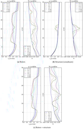
Figure 13.
Vertical profiles of time-averaged velocity magnitude and turbulence intensity for rotors, structure and rotors with structure. The units for x are D, i.e., the rotor diameter (=16 m).
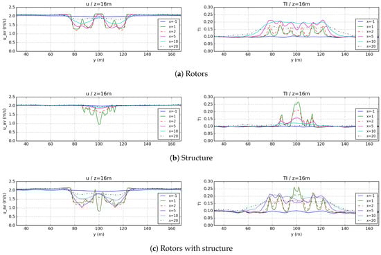
Figure 14.
Horizontal transects of time-averaged velocity and turbulence intensity at z = 16 m for each full-scale case. Units for x are D.
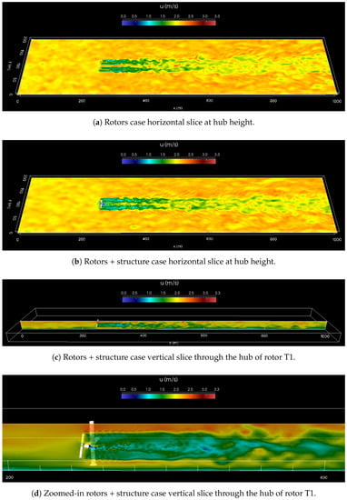
Figure 15.
Instantaneous snapshots of the velocity field for rotor and rotor+structure cases, at the end of the simulation.
For the structure-only case (Figure 13a and Figure 14c), the velocity profiles show a sharp drop immediately behind the crossbeam, with nearly full velocity recovery by 5 D. The horizontal-transect profiles are more complicated, as the transect is at hub-height (z = 16 m), and crosses in front of (and behind) the tower, as well as the upper, outer ends of the crossbeam (cf. Figure 10). Furthermore, the nacelles exert a strong influence on turbulence levels, raising the TI to 17.5% at 1 D, 13% at 5 D, before approaching background levels by 10 D. At 20 D, the difference between upstream TI values is negligible.
The velocity profiles for the rotors + structure case (Figure 13c and Figure 14a) are broadly similar to the rotors-only case, but with several important differences. Firstly, the pronounced peak visible in the rotors-only profile (Figure 13a and Figure 14a) has been replaced with flatter troughs. This is due to the influence of the crossbeam and the nacelle sections, causing the flow to accelerate around the solid structure, rather than through the empty hub volume in the rotors as before. This effect can be observed in the instantaneous vertical velocity snapshots in Figure 15c,d (zoomed in). Secondly, the flattened velocity peak in the horizontal transects between the rotors no longer occurs at 1 D, owing to the presence of the monopile and crossbeam. Instead, two sharp spikes can be seen at approximately , either side of the central trough at 0.8 . By 5 D downstream, these have become one peak at 1.8 , somewhat lower than in the rotors case (2.2 ). This pattern continues at 10 D and 20 D; the velocity profiles are similar, but0.1–0.2 lower in the rotors and structure regions. The horizontal velocity snapshot in Figure 15b reflects this, with the pronounced central jet between the rotor wakes in Figure 15a no longer visible. As expected, the vertical TI profile in Figure 13c is broadly similar to that in Figure 13a, but higher turbulence levels occur downstream, particularly behind the structure. At 1 D, the TI is between 20 and 25% near the nacelle region, much higher than the 12–17% for the rotors only. By 10 D, however, TI profiles from both the rotors-only and rotors + structure cases are nearing equivalence. Lastly, of particular note are the TI peaks at the rotor tips, visible in Figure 13c and Figure 14c, which are 16–40% larger than the rotors’ case. This suggests that the blades themselves may be subject to, and causing, fluctuations in the flow. Turbulence spectra were calculated at a point 1 D downstream from top of rotor T1 for both cases (cf. Figure 16), which confirm that while both exhibit a peak at 0.4 Hz, this is particularly pronounced when the structure is included. We explore this further in Section 5.2.
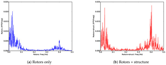
Figure 16.
Resolved turbulence spectra at 1D downstream from the top of the T1 rotor, for (a) the rotors case and (b) rotors + structure. Both cases show a second peak at 0.4 Hz, with the peak four-times higher in the rotors + structure case.
5.2. Turbine Diagnostics
Here, we examine how the performance of the turbine is affected by the absence or inclusion of the support structure. Figure 17 presents a selection of diagnostics from the rotors-only test, which show that the power from each rotor fluctuates semi-independently of the other, due to the unsteady, turbulent flow each rotor experiences. We use the term ‘semi-independently’, because some of the eddies are large enough for each rotor to experience them simultaneously. For both rotors T1 and T2, power output varies approximately kW from their mean values. The mean power outputs for T1 and T2 differ by 0.25%; for simulations of longer duration, these should converge. The weighted angle of attack along the blades, , shows much less variation, as the pitch control mechanism tries to maximise power output [4,60]. The results from the rotors + structure case are broadly similar.
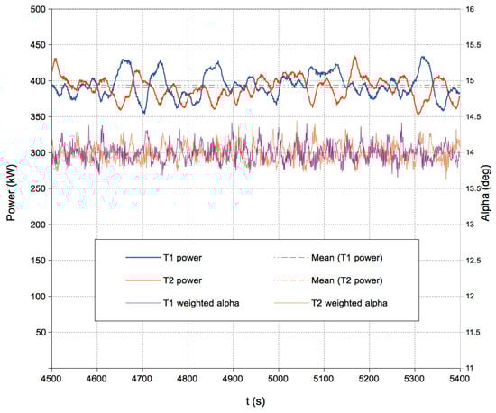
Figure 17.
Diagnostic output from both rotors, T1 and T2, showing power, and , the weighted mean angle of attack (see Creech et al. [4] for details) for each. The dashed lines indicate mean power output.
The net time-averaged power output of cases for the single rotor, both rotors only and then the rotors + structure are compared against published measurements for SeaGen in Table 3. The models are in close agreement, with a maximum error of 5.1%. It is particularly interesting that the simulations modelling both rotors have more accurately predicted the power output than the single rotor case, suggesting that there is interaction between the two rotors. This may be down to the blockage effects of each individual rotor, which accelerates flow round the edges of the rotors, in theory providing a small performance increase. Indeed, the acceleration effect can clearly discernible in Figure 14a.
Table 3.
Comparison of power output values.
Investigating the effect of the support structure on the power output, Table 3 indicates little difference between the rotors and rotors + structure cases, with errors of 4.4% and 4.7%, respectively. It is also worth examining the time series of the power output from each rotor, to see if there are any regular fluctuations as the blades pass in front of the supporting structure (such as the crossbeam). This was achieved by applying fast-Fourier transforms (FFT) to the power output. As there was a short sampling period (900 s) and the likelihood of similar spectral characteristics in fluctuations in each rotor, for each simulation, FFTs of the power time series for each rotor were calculated separately and then the average taken. Figure 18 displays these for the rotors case and the rotors + structure case. Towards the lower end of the frequency range, both plots become noisy, as longer wavelengths are not resolved satisfactorily within the sampling period. In Figure 18a, the rotors only case, there is a small peak at 0.4 Hz; however, in Figure 18b, when the structure is added, the peak at the same frequency is much larger. The mean rotational frequency of the rotors in one simulation is defined as:
where is a time-averaged rotor angular velocity from the diagnostics data for rotor .
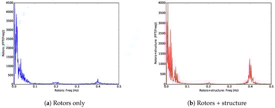
Figure 18.
Rotor-averaged FFT plots of the power time-series, for (a) rotors only and (b) rotors + structure. There is a pronounced spike at 0.4 Hz for the simulation that includes the support structure.
The values for the frequencies in Table 4 demonstrate that both cases are identical to within four significant figures. It should be noted that is almost exactly half of 0.4 Hz, shown in Figure 18a,b. This is not surprising, given there are two blades. To determine where in the rotation cycle these high-frequency power fluctuations occur, the low frequencies were removed using a Hamming window function, with spectral inversion used to create a high-pass filter. The cut-off frequency was 0.3 Hz, with a transition bandwidth of 0.05 Hz. The position of the first blade was then plotted against these fluctuations for each turbine. For comparison, the same process was carried for the case with rotors only, and the graphs for both are shown in Figure 19.
Table 4.
Mean rotational frequencies of the rotors in each simulation case.
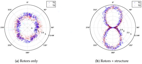
Figure 19.
Polar plots of blade position versus power fluctuations above 0.3 Hz, for rotors T1 and T2, in (a) the rotors-only simulation and (b) including the structure. 0° means the blade is pointing upwards, and power fluctuations are plotted from −7.5–7.5 kW. T1 rotates anti-clockwise and T2 rotates clockwise. The extent of the power fluctuations is approximately ±7.5 kW in (b), whereas in (a) it is a third of the size, at ±2.5 kW.
Figure 19a shows that in the rotors-only case, the power fluctuations have a relatively even spread within a range of ± 2.5 kW, with slightly higher values when either blade points upwards at 0. This increase is most likely due to the higher flow speeds and thus the lift that the blades experience at 0, as shown in the vertical velocity profile in Figure 13a. Discrepancies between this and the rotor + structure case are quite evident from Figure 19b, where a clear pattern emerges, with fluctuations peaking at a maximum of 7.5 kW at a blade position of 0 and 180 and at a minimum of −7.5 kW at 90 and 270. Table 5 lists these in terms of mean total output per rotor. It is clear that in the rotors + structure simulation, a dip in power output is experienced when the blades are aligned with the cross-beam. By comparing the horizontal velocity profiles at hub height in Figure 14a,c, just downstream of the rotors at x = 1 D, the velocity deficits are more pronounced when the structure is included. In particular, the absence of the nacelles and tower is noticeable, with a peak flow speed of 1.75 in the rotors-only case at y = 87 m and y = 113 m and at y = 100 m, where the nacelles and tower would be, respectively. This can be attributed to the blockage effect, created by the back thrust of the rotors, causing the flow to accelerate around the rotors and through the centre where the lift is reduced. In contrast, the velocity profiles in Figure 14c show no accelerated flow at the nacelles, and the velocity deficit created by the wake of the tower reaches 0.8 , compared to the rotors-only case, which peaks at 2.2 , i.e., . The culmination of the upstream effect of the supporting structure, in terms of the turbine performance, is a periodic fluctuation in power, responsible for a variation in output of almost 4%. Blade loading has not been analysed, but it can be expected to have more variation than power, due to the system inertia smoothing out fluctuations in power. The effect of inertia on power output can be seen in the slight asymmetries of the polar plot in Figure 19b.
Table 5.
High frequency power fluctuation ranges for rotor and rotor + structure cases.
6. Discussion and Conclusions
Large Eddy simulation has been used to model a full-scale, dual rotor, contra-rotating turbine, complete with structure, in a realistic-sized channel domain. The results demonstrate that the structure does have a noticeable effect on performance and the near-wake, causing regular fluctuations in both power output and flow speed.
There are few CFD models of dual rotor configurations in modelling literature. Of these, the tidal turbine array LES simulations of Churchfield et al. [8], show similarities in the downstream wake profiles; however, their domain was less than a quarter of the size of the channel domain used here, and so, their results may be subject to exaggerated blockage effects due to the proximity of the domain walls. Furthermore, they did not use synthetic eddy methods for realistic inlet turbulence, unlike the present paper. Closer comparisons may be drawn with Afgan et al. [27] and Ahmed et al. [28], who used SSTRANS and also LES with SEM to model a resolved three-bladed rotor and the support structure. Their time-averaged LES results of the power coefficient exhibited regular pronounced fluctuations as a function of blade angle with the rotors upstream; in the RANS simulations, these were absent. The RANS models of Mason-Jones et al. [67], however, did predict increased fluctuations in torque with blade angle when the stanchion supporting the turbine was included. The lesson here is that care must be used when deploying RANS turbulence schemes to capture transient behaviour in diagnostics. Moreover, the flow direction experiments of Frost et al. [68] showed that individual blade thrusts varied considerably with blade angle upstream, whereas net rotor thrust and power output did not. It must be noted that their turbine configuration differs somewhat from our model, having three blades with one central monopile, versus our dual two-bladed, crossbeam-mounted arrangement. Although there are valuable advances in research using actuator disc approaches [24,26,69,70], particularly in terms of tidal farm modelling, the discretisation of the blades into continuous rings means that such models cannot capture the same fluctuations in power output due to blade-structure interaction. Whether or not this is important for the far-wake of tidal turbines remains an open question, but for mechanical and electrical reliability, these transient features must either be represented or parameterised for accurate simulation.
In terms of wake prediction, measurements from a full-scale turbine would have been useful for model validation. As with the technical specifications; however, ADCP measurements of SeaGen’s downstream wake were unavailable, so comparison is instead made with the experimental and numerical literature. The water channel tests of Myers and Bahaj [71], despite being of scaled single rotor turbine, support the results in Figure 13b and Figure 14c that show that the structure alone creates substantial turbulence even at 5 D downstream. With the rotors included; our findings agree with those of Batten et al. [25], and Stallard et al. [72,73], in that at 20 D (22 D in Batten), the turbine wake had still not recovered to its original value. They too report higher than background readings for turbulence intensity far downstream. In the near wake, there is good agreement between the cross-stream turbulence profile in Figure 14c and Tedds et al. [74], both showing peaks of 20–25% 1–2 D downstream, as well as a peak at the centre near the structure. This is surprising, given the differences in geometry of both rotor and structure; indeed the difference in structure (single stanchion versus monopile + crossbeam for SeaGen) may account for the variance in the central peak. Such conformance across a range of scales and models is encouraging, given that levels of upstream turbulence have been found to influence tidal turbine performance [75]; the turbulence profiles in our rectilinear channel reflect a satisfactory approximation to a generic channel, but they do not reflect any particular tidal site.
The key finding of this paper is that the support structure has a discernible effect on the flow upstream, the downstream wake and turbine behaviour, for a contra-rotating, dual rotor tidal turbine. The behavioural changes manifest themselves as regular oscillations in the power output at twice the rotor rotational frequency and constitute 4% of total output. Furthermore, these fluctuations affect the near-wake of each rotor, where these oscillations are evident in the turbulence spectra, and so undoubtedly causing regular variations in structural loading. Inclusion of the structure in simulations also produces deeper, more persistent wake deficits, as well as substantially higher levels of turbulence downstream, well into the far wake. These results are somewhat dependent on the SeaGen model design, and differences can be expected between it and more conventional single-rotor devices. These matters bear further investigation, particularly for tidal turbine arrays. Whilst array layouts were beyond the scope of the research presented here, it is recommended that future work should investigate the consequences of the resultant complicated wake flows, for the electrical and mechanical systems of tidal turbines. In summary, the present study confirms that if the support structure and individual rotors are not resolved or parameterised appropriately within a numerical model, then the results of such simulations should be held in doubt, from the interrelated perspectives of turbine reliability, performance and fluid dynamics.
Acknowledgments
This research was supported through Natural Environment Research Council (U.K.) Grant NE/J004332/1 on the joint project ‘FLOWBEC - FLOW and Benthic ECology 4D’, with additional support from Engineering and Physical Sciences Research Council (U.K.) Grant EP/M014738/1 ‘Extension of UKCMER Core Research, Industry and International Engagement’. We also acknowledge the support of 10 MAUs of computing time on ARCHER, the U.K. national academic supercomputer. Finally, we would like to thank Peter Fraenkel for his invaluable contributions and insights into tidal turbine design.
Author Contributions
A.C.W.C. conceived of the research, designed and ran the simulations, analysed the data and wrote the paper. A.G.L.B. contributed ideas to the research. A.G.L.B. and D.I. contributed revisions to the paper.
Conflicts of Interest
The authors declare no conflict of interest.
References
- Jensen, N. A Note on Wind Generator Interaction; Technical Report; Risø National Laboratory: Roskilde, Denmark, 1983. [Google Scholar]
- Jimenez, A.; Crespo, A.; Migoya, E.; Garcia, J. Large-eddy simulation of spectral coherence in a wind turbine wake. Environ. Res. Lett. 2008, 3, 015004. [Google Scholar] [CrossRef]
- Wu, Y.T.; Porte-Agel, F. Large-Eddy Simulation of Wind-Turbine Wakes: Evaluation of Turbine Parametrisations. Bound. Layer Meteorol. 2011, 138, 345–366. [Google Scholar] [CrossRef]
- Creech, A.C.W.; Früh, W.G.; Maguire, A.E. Simulations of an offshore wind farm using large eddy simulation and a torque-controlled actuator disc model. Surv. Geophys. 2015, 36, 427–481. [Google Scholar] [CrossRef]
- Sørensen, J.; Shen, W. Numerical modelling of wind turbine wakes. J. Fluids Eng. 2002, 124, 393–399. [Google Scholar] [CrossRef]
- Troldborg, N.; Sorensen, J.; Mikkelsen, R. Numerical simulations of wake characteristics of a wind turbine in uniform inflow. Wind Energy 2010, 13, 86–99. [Google Scholar] [CrossRef]
- Churchfield, M.J.; Lee, S.; Moriarty, P.J.; Martínez, L.A.; Leonardi, S.; Vijayakumar, G.; Brasseur, J.G. A Large-Eddy Simulation of Wind-Plant Aerodynamics. In Proceedings of the 50th AIAA Aerospace Sciences Meeting, Nashville, Tennessee, 9–12 January 2012. [Google Scholar]
- Churchfield, M.J.; Li, Y.; Moriarty, P.J. A Large-Eddy Simulation Study of Wake Propagation and Power Production in an Array of Tidal-Current Turbines. Philos. Trans. R. Soc. A 2013, 371, 1471–2962. [Google Scholar] [CrossRef] [PubMed]
- Porté-Agel, F.; Wu, Y.T.; Lu, H.; Conzemius, R.J. Large-eddy simulation of atmospheric boundary layer flow through wind turbines and wind farms. J. Wind Eng. Ind. Aerodyn. 2011, 99, 154–168. [Google Scholar] [CrossRef]
- Barthelmie, R.; Folkerts, L.; Rados, G.C.L.K.; Pryor, S.C.; Frandsen, S.T.; Lange, B.; Schepers, G. Comparison of Wake Model Simulations with Offshore Wind Turbine Wake Profiles Measured by Sodar. J. Atmos. Ocean. Technol. 2006, 23, 888–901. [Google Scholar] [CrossRef]
- Sanderse, B.; van der Pijl, S.; Koren, B. Review of computational fluid dynamics for wind turbine wake aerodynamics. Wind Energy 2011, 14, 799–819. [Google Scholar] [CrossRef]
- Creech, A.C.W.; Früh, W.G. Modelling wind turbine wakes for wind farms. Altern. Energy Shale Gas Encycl. 2016. [Google Scholar] [CrossRef]
- Wußow, S.; Sitzki, L.; Hahm, T. 3D-simulation of the turbulent wake behind a wind turbine. J. Phys. Conf. Ser. 2007, 75, 12036. [Google Scholar] [CrossRef]
- Früh, W.G.; Seume, J.; Gomez, A. Modelling the aerodynamic response of a blade passing in front of the tower. In Proceedings of the European Wind Energy Conference, Brussels, Belgium, 31 March–3 April 2008. [Google Scholar]
- Creech, A.C.W.; Früh, W.G.; Clive, P. Actuator volumes and hr-adaptive methods for 3D simulation of wind turbine wakes and performance. Wind Energy 2012, 15, 847–863. [Google Scholar] [CrossRef]
- Creech, A.C.W.; Früh, W.G.; Maguire, A.E. High-resolution CFD modelling of Lillgrund Wind farm. Renew. Energies Power Qual. J. 2013, 11, 983–988. [Google Scholar] [CrossRef]
- Adcock, T.; Draper, S.; Houlsby, G.; Borthwick, A.; Serhadlıoǧlu, S. The available power from tidal stream turbines in the Pentland Firth. Proc. R. Soc. A 2013. [Google Scholar] [CrossRef]
- Coles, D.S.; Blunden, L.S.; Bahaj, A.S. Resource Assessment of Large Marine Current Turbine Arrays. J. Ocean Eng. 2013. [Google Scholar] [CrossRef]
- Plew, D.; Stevens, C. Numerical modelling of the effect of turbines on currents in a tidal channel—Tory Channel, New Zealand. Renew. Energy 2013, 57, 269–282. [Google Scholar] [CrossRef]
- Funke, S.; Farrell, P.; Piggott, M. Tidal turbine array optimisation using the adjoint approach. Renew. Energy 2014, 63, 658–673. [Google Scholar] [CrossRef]
- Lawson, M.; Li, Y.; Sale, D. Development and verification of a computational fluid dynamics model of a horizontal-axis tidal current turbine. In Proceedings of the 30th International Conference on Ocean, Offshore and Arctic Engineering, Rotterdam, The Netherlands, 19–24 June 2011. [Google Scholar]
- Shi, W.; Wang, D.; Atlar, M.; Seo, K.C. Flow separation impacts on the hydrodynamic performance analysis of a marine current turbine using CFD. Proc. IMechE Part A J. Power Energy 2013, 227, 833–846. [Google Scholar] [CrossRef]
- Creech, A.C.W. A Three-Dimensional Numerical Model of a Horizontal Axis, Energy Extracting Turbine. Ph.D. Thesis, Heriot-Watt University, Edinburgh, UK, 2009. [Google Scholar]
- Nishino, T.; Willden, R. Effects of 3-D channel blockage and turbulent wake mixing on the limit of power extraction by tidal turbines. Int. J. Heat Fluid Flows 2012, 37, 123–135. [Google Scholar] [CrossRef]
- Batten, W.M.J.; Harrison, M.; Bahaj, A.S. The accuracy of the actuator disc-RANS approach for predicting the performance and wake of tidal turbines. Philos. Trans. R. Soc. A 2013, 371. [Google Scholar] [CrossRef] [PubMed]
- Masters, I.; Williams, A.; Croft, T.; Togneri, M.; Edmunds, M. A Comparison of Numerical Modelling Techniques for Tidal Stream Turbine Analysis. Energies 2015, 8, 7833–7853. [Google Scholar] [CrossRef]
- Afgan, I.; McNaughton, J.; Rolfo, S.; Apsley, D.D.; Stallard, T.; Stansby, P.K. Turbulent flow and loading on a tidal stream turbine by LES and RANS. Int. J. Heat Fluid Flow 2013, 43, 96–108. [Google Scholar] [CrossRef]
- Ahmed, U.; Afgan, I.; Apsley, D.; Stallard, T.; Stansby, P.K. CFD Simulations of a Full-Scale Tidal Turbine: Comparison of LES and RANS with Field Data; EWTEC: Nantes, France, 2015. [Google Scholar]
- McNaughton, J.; Afgan, I.; Apsley, D.D.; Rolfo, S.; Stallard, T.; Stansby, P.K. A simple sliding-mesh interface procedure and its application to the CFD simulation of a tidal-stream turbine. Int. J. Numer. Methods Fluids 2014, 74, 250–269. [Google Scholar] [CrossRef]
- Piggott, M.; Pain, C.; Gorman, G.; Power, P.; Goddard, A. h, r, and hr adaptivity with applications in numerical ocean modelling. Ocean Model. 2004, 10, 95–113. [Google Scholar] [CrossRef]
- Baliga, B.; Patankar, S. A New Finite-Element Formulation for Convection-Diffusion Problems. Numer. Heat Transf. 1980. [Google Scholar] [CrossRef]
- Smagorinsky, J. General Circulation Experiments with the Primitive Equations. Mon. Weather Rev. 1963, 91. [Google Scholar] [CrossRef]
- Deardroff, J.W. A numerical study of three-dimensional turbulent channel flow at large Reynolds numbers. J. Fluid Mech. 1970, 41, 453–480. [Google Scholar] [CrossRef]
- Bull, J.R.; Piggott, M.; Pain, C. A finite element LES methodology for anisotropic inhomogeneous meshes. Turbul. Heat Mass Transf. 2012, 7, 1–12. [Google Scholar]
- Scotti, A.; Meneveau, C. Generalized Smagorinsky model for anisotropic grids. Phys. Fluids A 1993, 5, 2306–2308. [Google Scholar] [CrossRef]
- Bentham, T. Microscale Modelling of Air Flow and Pollutant Dispersion in the Urban Environment. Ph.D. Thesis, Imperial College London, Kensington, UK, 2003. [Google Scholar]
- Keenan, G.; Sparling, C.H.W.; Fortune, F. SeaGen Environmental Monitoring Programme; Technical Report; Royal HaskoningDHV: Amersfoort, The Netherlands, 2011. [Google Scholar]
- Rippeth, T.; Williams, E.; Simpson, J. Reynolds Stress and Turbulent Energy Production in a Tidal Channel. J. Phys. Oceanogr. 2001, 32, 1242–1251. [Google Scholar] [CrossRef]
- Jarrin, N.; Benhamadouche, S.; Laurence, D.; Prosser, R. A synthetic-eddy-method for generating inflow conditions for large-eddy simulations. Int. J. Heat Fluid Flows 2006, 27, 585–593. [Google Scholar] [CrossRef]
- Nezu, I.; Nakagawa, H. Turbulence in Open Channel Flows; Balkema: Rotterdam, The Netherlands, 1993. [Google Scholar]
- Milne, I.; Sharma, R.; Flay, R.; Bickerton, S. Characteristics of the Onset Flow Turbulence at a Tidal-Stream Power Site. In Proceedings of the 9th European Wave and Tidal Energy Conference, Southampton, UK, 5–9 September 2011. [Google Scholar]
- Stacey, M.; Monismith, S.; Burau, J. Measurements of Reynolds stress profiles in unstratified tidal flow. J. Geophys. Res. 1999, 104, 10933–10949. [Google Scholar] [CrossRef]
- Bryden, I.G.; Couch, S.J.; Owen, A.; Melville, G. Tidal current resource assessment. Proc. IMechE Part A J. Power Energy 2007, 221, 125–135. [Google Scholar] [CrossRef]
- Bearhop, S.; Elsasser, B.; Inger, R.; Pritchard, D. Chapter Strangford Lough and the SeaGen tidal turbine. In Marine Renewable Energy Technology and Environmental Interactions; Springer: Dordecht, The Netherlands, 2014; pp. 153–172. [Google Scholar]
- Delany, N.K.; Sorensen, N.E. Low-Speed Drag of Cylinders of Various Shapes; Technical Report Technical Note 3038; National Advisory Committee for Aeronautics: Washington, DC, USA, 1953. [Google Scholar]
- Thom, A. The Forces on a Cylinder in Shear Flow; Technical Report; Ministry of Aviation: UK, 1963.
- Shih, W.; Wang, C.; Coles, D.; Roshko, A. Experiments on flow past rough circular cylinder at large Reynolds numbers. J. Wind Eng. Ind. Aerodyn. 1993, 49, 351–368. [Google Scholar] [CrossRef]
- Mackwood, P.; Bearman, P.; Graham, J. Wave and Current Flows Around Circular Cylinders at Large Scale; HSE Books: UK, 1998. [Google Scholar]
- Chaplin, J.; Teigen, P. Steady flow past a vertical surface-piercing circular cylinder. J. Fluids Struct. 2003, 18, 271–285. [Google Scholar] [CrossRef]
- Cabot, W.; Moin, P. Approximate Wall Boundary Conditions in the Large-Eddy Simulation of High Reynolds Number Flow. Flow Turbul. Combust. 2000, 63, 269–291. [Google Scholar] [CrossRef]
- Wang, M.; Catalano, P.; Iaccarino, G. Prediction of High Reynolds Number Flow over a Circular Cylinder Using LES with Wall Modeling; Technical report; Center for Turbulence Research: Stanford, CA, USA, 2001. [Google Scholar]
- Ochoa, J.; Fueyo, N. Large Eddy Simulation of the flow past a square cylinder. In Proceedings of the PHOENICS 10th International User Conference, Melbourne, Australia, 3–5 May 2004. [Google Scholar]
- Fraenkel, P. Marine current turbines: pioneering the development of marine kinetic energy converters. Proc. IMechE Part A J. Power Energy 2007, 221, 159–169. [Google Scholar] [CrossRef]
- Roshko, A. Experiments on the flow past a circular cylinder at very high Reynolds number. J. Fluid Mech. 1961, 10, 345–356. [Google Scholar] [CrossRef]
- Jones, G.; Cincotta, J.; Walker, R. Aerodynamic Forces on a Stationary and Oscillating Circular Cylinder at High Reynolds Numbers; Technical Report NASA TR R-300; NASA: Washington, DC, USA, 1969.
- Achenbach, E. Distribution of local pressure and skin friction around a circular cylinder in cross-flow up to Re = 5 × 10⁶. J. Fluid Mech. 1968, 34, 625–639. [Google Scholar] [CrossRef]
- Creech, A.C.W. GitHub source code repository for Wind And Tidal Turbine Embedded Simulator (WATTES). Available online: https://github.com/wattes (accessed on 18 May 2017).
- Burton, T.; Sharpe, D.; Jenkins, N.; Bossanyi, E. Wind Energy Handbook; Wiley: Oxford, UK, 2006. [Google Scholar]
- Bedard, R. TP-004-NA: Survey and Characterization of TISEC Devices; Technical report; Electric Power Research Institute: Palo Alto, CA, USA, 2005. [Google Scholar]
- Fraenkel, P. Private communication, 2014.
- Fraenkel, P. Practical tidal turbine design considerations: A review of technical alternatives and key design decisions leading to the development of the SeaGen 1.2MW tidal turbine. In Proceedings of the Ocean Power Fluid Machinery Seminar (IMechE), London, UK, 19 October 2010. [Google Scholar]
- Myers, L.; Bahaj, A.S. Simulated electrical power potential harnessed by marine current turbine arrays in the Alderney Race. Renew. Energy 2005, 30, 1713–1731. [Google Scholar] [CrossRef]
- Douglas, C.A.; Harrison, G.P.; Chick, J.P. Life cycle assessment of the SeaGen marine current turbine. Proc. IMechE Part M J. Eng. Maritime Environ. 2008, 222, 1–12. [Google Scholar] [CrossRef]
- Neill, S.; Couch, E.L.S.; Davies, A. The impact of tidal stream turbines on large-scale sediment dynamics. Renew. Energy 2009, 34, 2803–2812. [Google Scholar] [CrossRef]
- Bertagnolio, F.; Sørensen, N.; Johansen, J.; Fuglsang, P. Wind Turbine Airfoil Catalogue; Technical Report Risø-R-1280(EN); Risø National Laboratory: Roskilde, Denmark, 2001. [Google Scholar]
- MacEnri, J.; Reed, M.; Thiringer, T. Influence of tidal parameters on SeaGen flicker performance. Philos. Trans. R. Soc. A 2013. [Google Scholar] [CrossRef] [PubMed]
- Mason-Jones, A.; O’Doherty, D.; Morris, C.; O’Doherty, T. Influence of a velocity profile & support structure on tidal stream turbine performance. Renew. Energy 2013, 52, 23–30. [Google Scholar]
- Frost, C.; Morris, C.; Mason-Jones, A.; O’Doherty, D.; O’Doherty, T. The effect of tidal flow directionality on tidal turbine performance characteristics. Renew. Energy 2015, 78, 609–620. [Google Scholar] [CrossRef]
- Hunter, W.; Nishino, T.; Willden, R. Investigation of tidal turbine array tuning using 3D Reynolds-Averaged Navier-Stokes Simulations. Int. J. Mar. Energy 2015, 10, 39–51. [Google Scholar] [CrossRef]
- Olczak, A.; Stallard, T.; Feng, T.; Stansby, P.K. Comparison of a RANS blade element model for tidal turbine arrays with laboratory scale measurements of wake velocity and rotor thrust. J. Fluids Struct. 2016, 64, 87–106. [Google Scholar] [CrossRef]
- Myers, L.; Bahaj, A.S. Near Wake Properties of Horizontal Axis Marine Current Turbines; EWTEC: Uppsala, Sweden, 2009. [Google Scholar]
- Stallard, T.; Collings, R.; Feng, T.; Whelan, J.I. Interactions between tidal turbine wakes: experimental study of a group of 3-bladed rotors. Philos. Trans. R. Soc. A 2013, 371, 20120159. [Google Scholar] [CrossRef] [PubMed]
- Stallard, T.; Feng, T.; Stansby, P.K. Experimental study of the mean wake of a tidal stream rotor in a shallow turbulent flow. J. Fluids Struct. 2015, 54, 235–246. [Google Scholar] [CrossRef]
- Tedds, S.; Owen, I.; Poole, R. Near-wake characteristics of a model Horizontal axis tidal stream turbine. Renew. Energy 2014, 63, 222–235. [Google Scholar] [CrossRef]
- Mycek, P.; Gaurier, B.; Germain, G.; Pinon, G.; Rivoalen, E. Experimental study of the turbulence intensity effects on marine current turbines behaviour. Part I: One single turbine. Renew. Energy 2014, 66, 729–746. [Google Scholar] [CrossRef]
© 2017 by the authors. Licensee MDPI, Basel, Switzerland. This article is an open access article distributed under the terms and conditions of the Creative Commons Attribution (CC BY) license (http://creativecommons.org/licenses/by/4.0/).