Article

Comparative Energy Performance Analysis of Six Primary Photovoltaic Technologies in Madrid (Spain)

by
Teodoro Adrada Guerra
1,*,
Julio Amador Guerra
1,
Beatriz Orfao Tabernero
2 and
Guillermo De la Cruz García
3
1
ETS Ingeniería y Diseño Industrial (ETSIDI), Universidad Politécnica de Madrid (UPM), Ronda de Valencia 3, 28012 Madrid, Spain
2
Renewable Energy and Environment, Universidad Politécnica de Madrid, 28012 Madrid, Spain
3
Consultora de Energías Renovables S.A. (CONERSA), Renewable Energy and Environment, Universidad Politécnica de Madrid, 28012 Madrid, Spain
*
Author to whom correspondence should be addressed.
Energies 2017, 10(6), 772; https://doi.org/10.3390/en10060772
Submission received: 21 March 2017 / Revised: 21 March 2017 / Accepted: 9 May 2017 / Published: 1 June 2017

Abstract

:
There are a wealth of studies on photovoltaic cell technologies, however their performance in different climatic or geographies over an extended period is not completely established. The objective of this paper is to add to this area of study with an analysis of the principle photovoltaic technologies: monocrystalline silicon (mc-Si), polycrystalline silicon (pc-Si), tandem structure of amorphous silicon and microcrystalline silicon (a-Si/µc-Si tandem), cadmium telluride/cadmium sulfide (CdTe/CdS), copper-indium diselenide (CIS) and monocrystalline silicon with double contact back technology (mc-dc-Si), in the climatic conditions particular to the middle latitude urban environment of Madrid (Spain). To carry out this study six photovoltaic subsystems of peak power 1 kWp approximately have been installed for each selected technology on the roof of the Escuela Técnica Superior de Ingeniería y Diseño Industrial (ETSIDI) of the Universidad Politécnica de Madrid (UPM) in Spain. Each subsystem has an inverter of the same model and power for its connection to the internal electricity network of the university. This paper analyzes the energy performance of the six subsystems, calculating the reference production rates and losses, from February 2013 to December 2015. The result of the study is the extensive capture of data and detailed analysis of real time energy yields and performance ratios of key technologies resulting with patterns in line with those of other regions with comparable climatic conditions.

1. Introduction

The calculation of the energy production of photovoltaic systems connected to the grid is a widely discussed topic [1,2,3,4,5,6,7,8], using detailed simulation models of its components [9,10,11,12,13,14,15,16,17] or more simplified methods [18,19,20,21,22,23,24,25]. There are a wide selection of meteorological databases that use these simulation programs such as AEMET [26], European Solar Radiation Atlas [27], NASA [28], METEONORM [29], ISPRA-GIS [30], HELIOS [31], SolarGIS [32], PV-Design Pro [33], etc., providing a basis for photovoltaic energy ratings in a variety of climatological conditions. It is important to note that there is uncertainty associated with the variability of solar radiation data used as a reference [34]. These programs predict performance ratios (PR) of between 75–90% when quality and well-sized materials and equipment are employed [7]. Commercial sizing programs such as PVSYST [9], PVSOL [16], SOLARPRO [17], etc., use the best available algorithms to evaluate and minimize energy losses caused by various causes, such as a selection of deficient components, shading, thermal losses, etc. Uncertainties related to different factors such as the relation between the real and nominal peak power of the photovoltaic modules [35,36], meteorological data, losses by dirt and shadowing, incidence angle, etc., provoke discrepancies between the predictions of the models and the real energy injected into the electric grid. The typical uncertainty range is usually between 0.5–2.5% [7].
The electrical characteristic parameters provided by manufacturers of photovoltaic modules have been obtained under standard test conditions (STC): irradiance 1000 W/m2, cell temperature 25 °C, air mass (AM) 1.5 and zero incidence angle; under normal operating cell (NOC): irradiance 800 W/m2, ambient temperature 20 °C and wind speed 1 m/s; and in conditions of low irradiance: irradiance 200 W/m2, cell temperature 25 °C and air mass (AM) 1.5. This information, including efficiency, is useful for comparing different technologies, but it does not provide complete information on the energy performance of the photovoltaic module at its installation site [37,38]. For this reason, IEC 61853-1:2011 [39] introduces two additional operating conditions, known as high and low temperature, high temperature condition (HTC) 1000 W/m2 and cell temperature 75 °C and low temperature condition (LTC) 500 W/m2 and cell temperature 15 °C. However, these last two operating conditions are not currently included in the vendor data sheets.
The reduction of the energy generated with respect to incident solar energy of a photovoltaic system can be explained by a set of factors: operating temperature of the modules [40,41,42,43,44,45,46,47,48], dirt and dust, partial shading of the modules, spatial arrangement, angular and spectral response of each technology [49,50,51,52,53,54,55], mismatch loss or connection between modules, non-compliance with the nominal power referred to STC conditions, the behavior of the inverter to work at the maximum power point of the photovoltaic generator and its loss of efficiency [56,57,58,59], the loss of power due to the degradation of the photovoltaic generator over time [60,61,62,63], ohmic drops in direct current and alternate current wiring, and by faults, breakdowns or the network connection.
Photovoltaic systems currently deployed have different energy efficiency rates depending on the cell technology, components, design and operating conditions. The conventional technologies of crystalline silicon cell (c-Si) usually have a higher temperature related power loss ~−0.45%/K with higher efficiencies in the winter than in the summer [5,41,43,44,64]. In the first hours of sun exposure the c-Si suffer power degradations of 0.5–1.5% [65,66,67] and have an annual power loss of 0.5–1%/year [44,60]. They are less sensitive to variation in the solar spectrum ~1–2% [49,51,55] and their angular losses can reach 3% [54].
Thin layer technologies have a more complex electrical characterization, especially for a-Si and HIT technologies [7,68]. Its nominal power tolerance can reach ±12% [47] and has a lower temperature related power loss coefficient −0.21 to −0.30%/K than conventional mc-Si and pc-Si technologies. They display higher efficiencies in the summer months, as is the case with a-Si and a-Si/µc-Si tandem technology, being optimum in hot or tropical climates [3,4,41,42,44,69,70]. Thin layer technologies take advantage of diffuse irradiation on cloudy days [52], have less dependence on the angle of inclination, but are more sensitive to variations in the solar spectrum, between 2–4% [1,55,68,71,72] than c-Si. The behavior of CIS and CdTe/CdS with solar irradiation and ambient temperature is similar to the c-Si with efficiency decreasing in the summer and increasing in the winter months [7,42,43,44,47]. The energy efficiency and life cycle of CIS and CdTe/CdS modules have been studied by Raugei et al. [62] demonstrating that these technologies can be competitive with respect to conventional technologies based on polycrystalline silicon.
A study carried out in 2010 by the manufacturer SUNPOWER [73] shows that the mc-dc-Si reaches an efficiency of around to 20.4% under STC conditions, has a lower power loss coefficient −0.38%/°C which is less than conventional c-Si, makes better use of diffuse irradiation and is less affected by the variation of the solar incidence angle and the air mass.
It is well known that thin layer technologies also undergo initial degradation in the first few hours or days of exposure to sunlight. The technology a-Si/µc-Si tandem suffers a degradation in the value of its nominal power that can reach 0.8% [69,74,75] until its stabilization. An opposite effect occurs with the CIS technology where in the first hours of operation there is a positive increase in efficiency 7–15% [68,75,76]. In the case of the CdTe/CdS the first few hours of solar exposure can increase efficiency by 6–8% or suffer degradation 7–15% [69,75,77] depending on the cell design and production process. In a five year study, Rodziewicz et al. [78] found that a-Si/µc-Si tandem technology had suffered a degradation of 10% of its nominal power, this value is higher than the loss suffered by mc-Si technology in the same period of time ~7%. Cañete et al. [43] have established in Malaga (Spain) in a yearlong study, that on certain days of high ambient temperature, that the daily efficiency drops to 5.4% for the CdTe, 6.5% for a-Si/µc-Si and 7.6% for pc-Si, compared to STC.
The inverter also has a significant influence on the energy injected into the grid with maximum efficiencies of 98%. Its efficiency is related to the value of the input voltage VDC and can produce variations of ±0.005 to 0.02%/V [59,79] depending on the type of inverter [80,81]. Network-connected inverters work with maximum power point tracking algorithms that try to maximize the energy produced by the photovoltaic generator [57,58]. As the point of maximum power changes with irradiation, temperature and shadows, there will be times when the inverter does not work at the point of maximum power.
On the other hand, in the real operating conditions of a photovoltaic installations there are incidents, breakdowns, disconnections to the grid, etc., which can affect energy production and this is why it is important to consider operative readiness. In a study of 78 photovoltaic installations in northern and eastern Germany [82] 63% of downtime was triggered by inverters, 15% by photovoltaic modules and 22% on failures of the rest of the components of the system.
In summary, energy generation of photovoltaic systems is affected by a large number of variables which need to be observed over an extended period of time. This paper shows the operation performance data of six primary photovoltaic technologies, in the climatic conditions particular to Madrid, from February 2013 to December 2015. The result is a detailed analysis of energy yields and performance ratios of these key technologies, displaying patterns in line with those of other regions with comparable climatic conditions.
Section 2 describes the photovoltaic systems under investigation. Section 3 presents and analyzes the recorded meteorological data. In Section 4 the energy parameters of each photovoltaic technology are defined and calculated, the results are presented in tables and graphs to facilitate their comparison. In Section 5, new energy parameters are defined and calculated taking into account the availability of each subsystem. Again tables and graphs are used to display the output permitting a better comparison of the performance of each type of photovoltaic technology. Section 5 is completed with an analysis of the evolution of operational efficiency. The study finishes with a summary of the findings and is followed by the complete bibliography.

2. Description of the Photovoltaic and Monitoring System

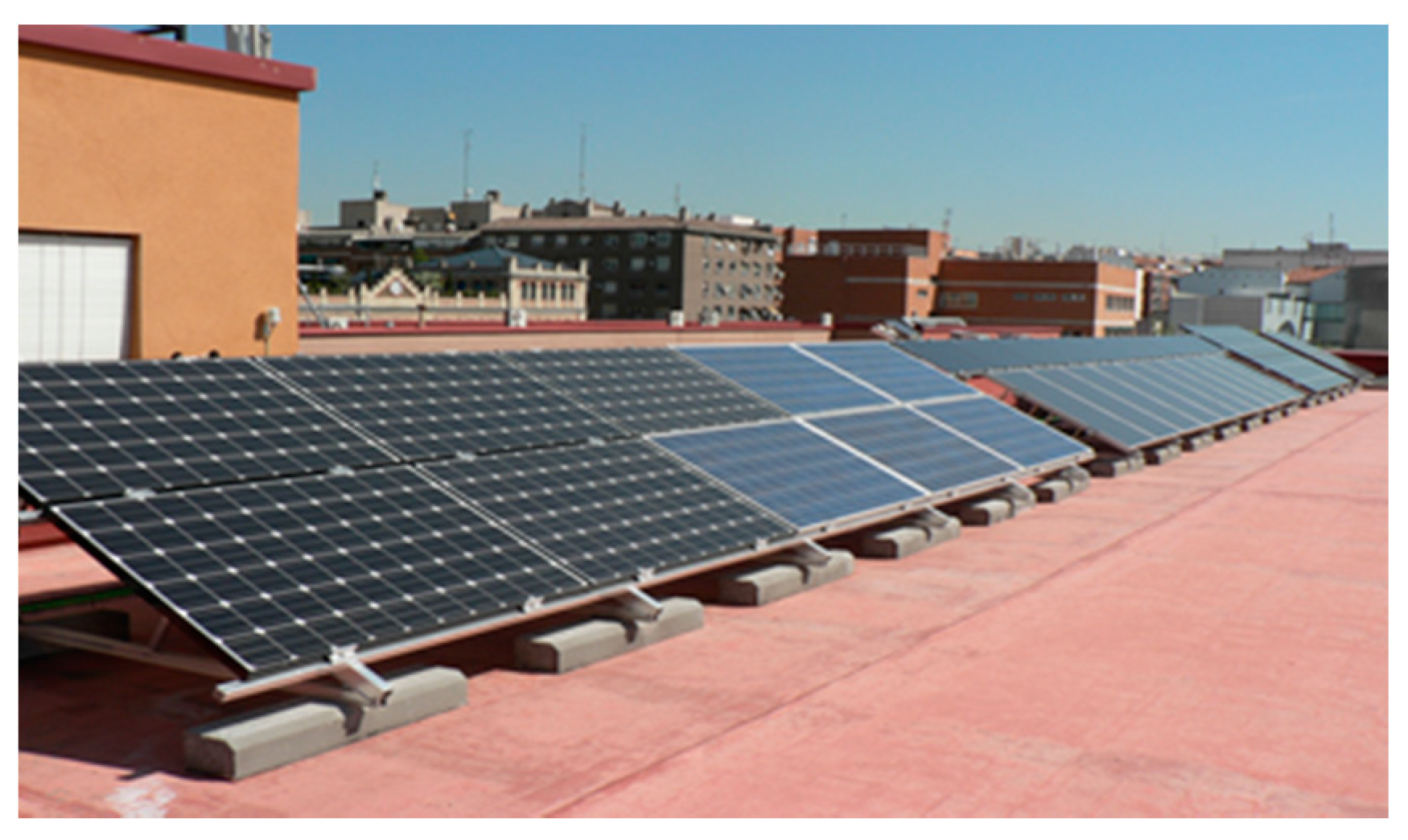
The photovoltaic system under study is installed in the main building of the Escuela Técnica Superior de Ingeniería y Diseño Industrial of the Universidad Politécnica de Madrid (ETSIDI-UPM): latitude 40.4°, longitude −3.7° and altitude 657 m. The building is in the center of the city of Madrid, where its flat roof is well exposed to solar radiation with shading of nearby buildings reduced to positions of the sun just after sunrise and before sunset. The site has a continental climate with cold winters and hot summers. The object of the investigation consists of 6 subsystems of different cell technologies: mc-Si, pc-Si, a-Si/µc-Si tandem, CdTe/CdS, CIS and mc-dc-Si mounted on weighted fixed tilt structures. All the modules of the different technologies are coplanar with a tilt of 30° and azimuth of 19° east to optimize the spatial distribution according to the architectural requirements of the roof. The structure provides a separation of 20 cm between the photovoltaic modules allowing natural cooling. The photovoltaic modules have been selected using models and manufacturers representative of each cell technology, Table 1 shows their main technical characteristics. All photovoltaic modules are conventional: glass top layer, white Tedlar backsheet and aluminum frame, except CdTe/CdS which has frameless glass to glass modules and CIS technology with glass to glass modules with frame. Table 2 describes the photovoltaic subsystems and Table 3 shows the main characteristics of the installed inverter, which is identical in all subsystems to facilitate performance comparison. A photograph of the photovoltaic system is shown in Figure 1.
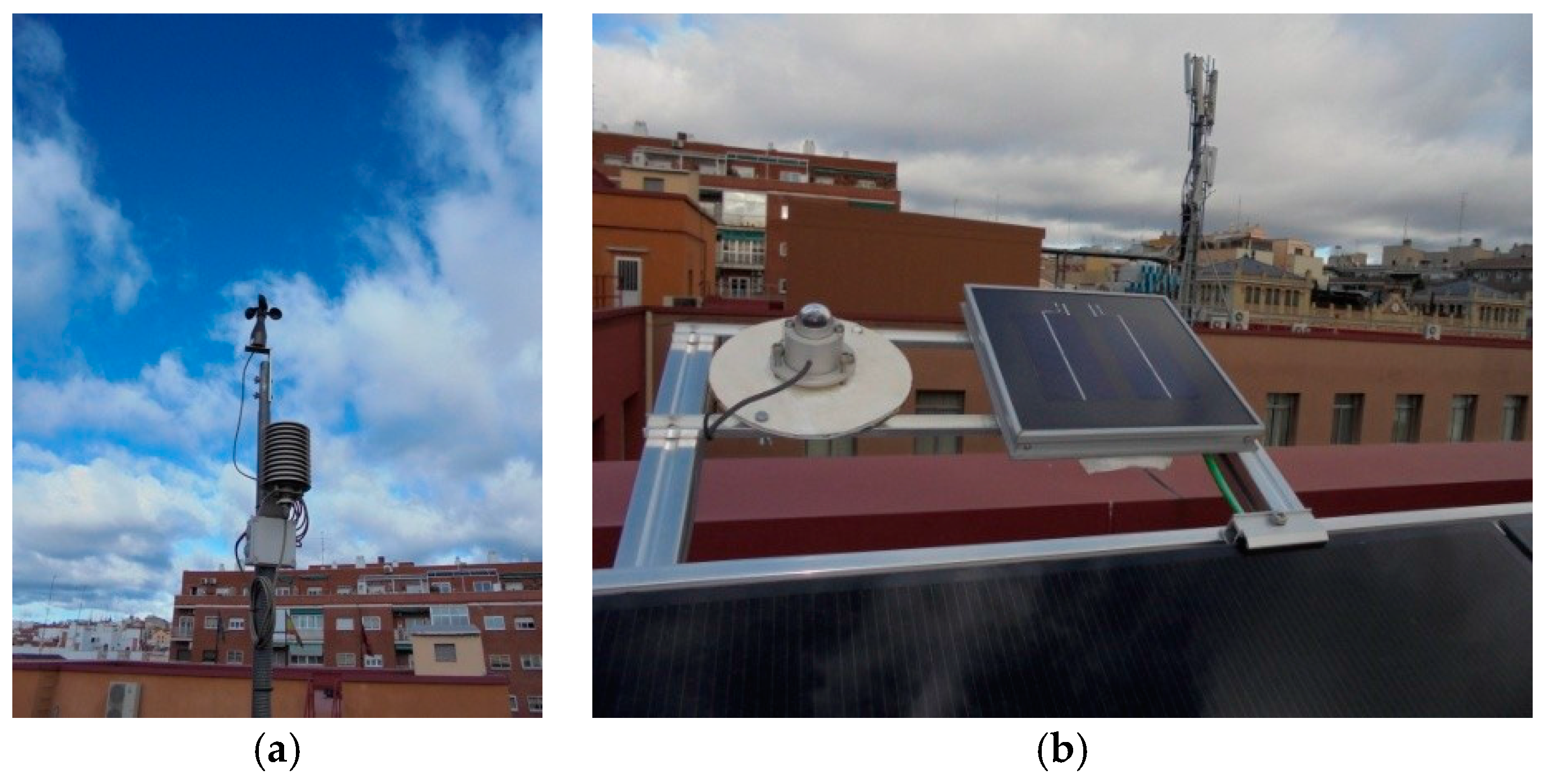
The influence of climatic variables on the performance of the photovoltaic systems are measured in accordance with Norm IEC 61724: 1998 and the guidelines of the Joint Research Center in Ispra, Italy [83,84,85]. The global solar irradiation (HI) (Wh/m2) data is captured by means of a thermoelectric pyranometer (PIR) and a calibrated reference cell (CRC) [
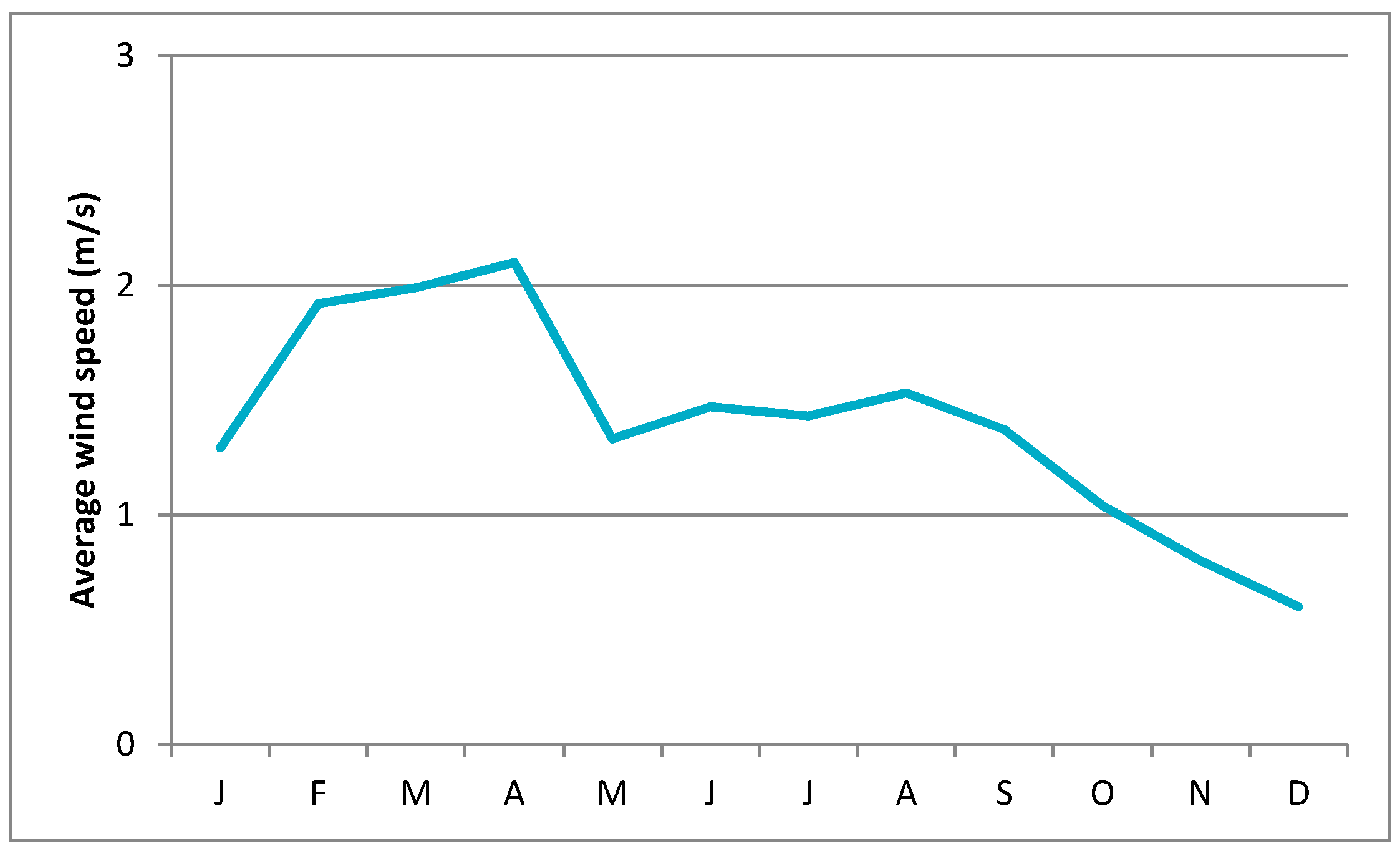
86] of polycrystalline silicon, both coplanar with the photovoltaic modules object of the investigation. The module temperature is measured with a PT-1000 thermocouple sensor fixed to the backsheet of a central cell, of one of the central modules of the array. Ambient temperature and relative humidity are measured with a thermohygrometer while wind speed uses an anemometer (Figure 2). The technical specifications of these sensors are shown in Table 4.
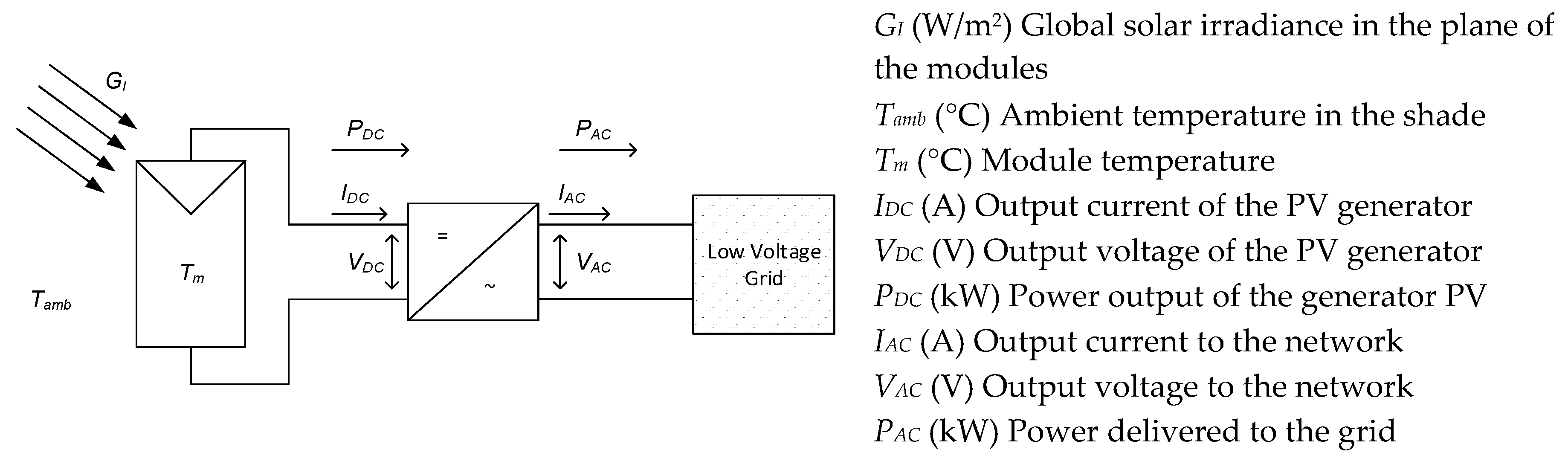
The electrical and meteorological variables (see Figure 3), are sampled every ten seconds with high precision Meteo Control Pro and IO web’log data loggers. The recording intervals are every five minutes, obtaining a representative average value for each interval. The measured electrical variables are taken from the inverters through the (recommended standard) RS-485 interface. Signal converters with 0.2 margin of error have been used for the meteorological variables including solar radiation, ambient temperature, relative humidity, wind speed and cells temperatures of the modules. This data can be consulted on the website CONERSA [87].

3. Meteorological Registered Data

3.1. Solar Irradiation

The mean values are obtained every five minutes with the pyranometer and the reference solar cell with an tilt of 30° and azimuth of 19° east, are contrasted with an average meteorological year (Table 5 and Figure 4) obtained from the Photovoltaic Geographic Information System (Ispra-PVGIS) [30]. The monthly values of the diffuse fraction of solar irradiation Dh/GI are taken from PVGIS and the HELIOS Solar Energy Institute (UPM) meteorological station [31] located 5 km away from the test site. Table 5 and Figure 4 show solar irradiation measurements and present small variations with respect to the average meteorological year. Clear sky conditions, low diffuse/global ratio Dh/GI ≈ 30% [7,86,88] found from June to September, produce the largest differences between the signals measured and those of HELIOS and the values of irradiation are higher in the pyranometer than the CRC. While in the winter months Dh/GI is close to ~45% the mean monthly irradiation values are similar for CRC and pyranometer (Table 5).
On average, the annual irradiation measured by CRC is ~2–4% lower than irradiance measured by pyranometers [86]. The spectral response of the CRC is usually between 0.3–1.1 µm, while the pyranometer is 0.3–3 µm [88] because the pyranometer has a broader spectral and angular response that leads to lower PR values especially in the summer months Figure 4. The CRC measurement of irradiation is more effective on days of mixed cloud cover because it has a shorter response time ≅ 1 ms to the pyranometer 5 to 20 s, demonstrating higher irradiance values [88]. The albedo effect needs to be taken into account since both devices are positioned with an inclination of 30° producing a systematic error in measured spectrum, being larger for the pyranometer. Higher performance values are obtained, especially in the summer months, when the calculations are measured by the CRC. This paper uses CRC measurements for the energy calculations.

3.2. Temperature of Operation of Modules

The energy production of each subsystem depends to a large extent on the operating cells temperature of the modules [40,41,42,43,44,45,46,47,48] which varies according to many factors: the ambient temperature (Tamb), the effective solar radiation, the wind speed [40,89], dirt that can cause hot spots and the characteristics of the installation. With the increase of the module temperature the open circuit voltage decreases and the short-circuit current rises slightly. Combining both effects results in a decrease in the peak power of the module. Figure 5 shows the mean monthly values of ambient temperature and temperature of the modules during the years 2013–2015, displaying a pattern in line with the local climatology.
Figure 5 shows that over practically the whole year the highest average module temperatures correspond to the CIS and CdTe/Cds technologies, both with glass to glass format, while the lowest correspond to the mc-cd-Si, with tedlar, although the differences are minimum (it should be noted that the mc-cd-Si modules are at the end of the rooftop and more exposed to airflows). Figure 6 shows the average monthly wind velocity values of one representative year. The anemometer is located 4 m high with respect to the position of the photovoltaic modules. The average wind speed in the summer months, with a higher solar irradiation and ambient temperature, is around 1.5 m/s so that its influence on the temperature of the modules can be considered of little relevance [89].

4. Energy Production of Photovoltaic Installation

Table 6 shows the energy production in kWh/year and in kWh/m2 for each subsystem in the study period.

4.1. Energy yield and Performance Ratio

In order to analyze the energy yield production indexes are calculated, according to Figure 7, of the standard IEC 61724: 98 [83] for each subsystem. Data is collated and available on databases around the world using production indexes of hundreds of photovoltaic systems located in different places and climatic conditions [7,82,90].
The available solar energy over a period of time T, is determined by the reference production index (YR) obtained dividing the global irradiance (GI) on the plane of the photovoltaic generator by the STC irradiance (GI,STC) (1 kW/m2) as per Equation (1):
Y R = T r T G I G I , S T C = H I G I , S T C
The array yield YA and the final yield YF for the period of time T, are calculated with Equations (2) and (3), respectively:
Y A = E D C P S T C
Y F = E A C P S T C
where: EAC = electricity generated by the photovoltaic system in kWh in period T; EDC = electricity generated at the input point of the inverter in kWh in period T; PSTC = nominal power of the photovoltaic generator STC conditions in kWp. The losses LC and LBOS can be obtained by Equations (4) and (5):
L C = Y R Y A
L B O S = Y A Y F
Figure 8a,b and Figure 9a,b show the monthly evolution of energy yields YA, YF and losses parameters LC and LBOS in kWh/kWpSTC without taking into account the operational availability for each subsystem over the studied period.
Figure 8a,b show the same evolution as YA and YF. The values of these two yields depend on certain meteorological conditions: solar radiation on the plane of the modules, ambient temperature and wind speed, which are the same for all the subsystems. These two indexes are related to the efficiency of the inverter according to Equation 9. This efficiency is very similar in all subsystems which use the same model of inverter and variations in the study period are minimal (see Section 4.3). Figure 9b follows a similar pattern, where the CdTe/CdS subsystem has declined since October 2014 and also suffered certain periods of inverter downtime. Figure 9a shows that the losses LC follow the same tendency as the temperatures of the modules, increasing in the summer months.
On the other hand, LC presents important differences between the different technologies. As the inverter is installed just behind the modules of the corresponding subsystem, losses in the DC wiring are negligible. The lowest losses are observed in CIS technology, and are even negative during the first two months of operation due to the increase at the initiation phase of the its efficiency [75], despite reaching highest module temperatures. The highest LC are observed in the CdTe/CdS technology from the outset and especially in the summer months. In the months of November and December of 2014 and January, May, June and July of 2015, there have been unexpected inverter stopages affecting drastically the value of YA.
The PR is calculated for the DC side (PRDC) and AC side (PRAC) using Equations (6) and (7). Normally the PR values are calculated on a monthly or annual basis [7,82,90]. Calculated values for smaller intervals, such as weekly or daily, can be useful for identifying faults in the components of the installation. Figure 10 and Figure 11 present the monthly evolution of PRDC and PRAC of all photovoltaic technologies in the years 2013, 2014 and 2015.
P R D C ( % ) = Y A Y R = E D C P S T C Y R × 100
P R A C ( % ) = Y F Y R = E A C P S T C Y R = Y R L c L B O S Y R = Y A L B O S Y R × 100
Due to losses to the photovoltaic modules caused by the temperature, the PRDC values are higher in winter than in summer, it is the inverse evolution to LC except in the a-Si/µc-Si tandem technology where the PRDC value is greater during summer [41,42,43,44]. Dirt in the photovoltaic modules will also affect the annual evolution of the PRDC [63]. A decrease in PRDC values over the three years is observed, caused by the loss of efficiency of photovoltaic generators due to their power degradation (see Section 4.4). The lowest decrease in PRDC in the three years is in mc-Si technology with 4%, followed by mc-dc-Si 5.2%, pc-Si 5.6% and a-Si/µc-Si 5.9%. CIS technology has decreased 9% and CdTe/CdS technology stands out with a decrease of 24.1%.

4.2. Photovoltaic Generator Efficiency

The efficiency of the photovoltaic generator is the ratio of the energy generated in EDC in kWh with respect to the incident irradiation (HI) in kWh/m2 during the same period of time T, multiplied by the capture area A in m2 according to Equation (8). The results are shown in Table 7.
η G ( % ) = E D C H I · A · 100
The loss of efficiency in the three years studied (ΔηG) varies depending on the technology, with the extreme values for CIS 1.6% and 4.7% for CdTe/CdS.

4.3. Inverter Efficiency

Once input EDC and output EAC energy of the inverters are known, the conversion efficiency of each inverter can be calculated as per Equation (9):
η i n v ( % ) = E A C E D C · 100 = Y F Y A × 100
The average annual inverter efficiency obtained during operation Table 8 have remained close to 90% in the three years of study and for all subsystems, so their contribution has been homogeneous, thus facilitating the comparison of the different photovoltaic technologies.
Table 8 shows that the efficiencies of the inverters are in line with the vendor data of 90.9–92.1% European efficiency rates, except for the inverters of subsystems 4 and 5 which are 0.7% and a 0.4% less, respectively.

4.4. Global Energy Efficiency

The global energy efficiency of each of the subsystems Figure 12, is calculated as the product of the efficiencies of the photovoltaic generator and the inverter according to Equation (10). Figure 12 shows the efficiency of each technology and effects of aging:
η G l o b a l ( % ) = η G · η i n v
The values of the calculated global efficiencies of the photovoltaic systems depend mainly on the initial nominal efficiency ratings and their reductions are in line with the usual power degradation corresponding to each technology [43,44,60].

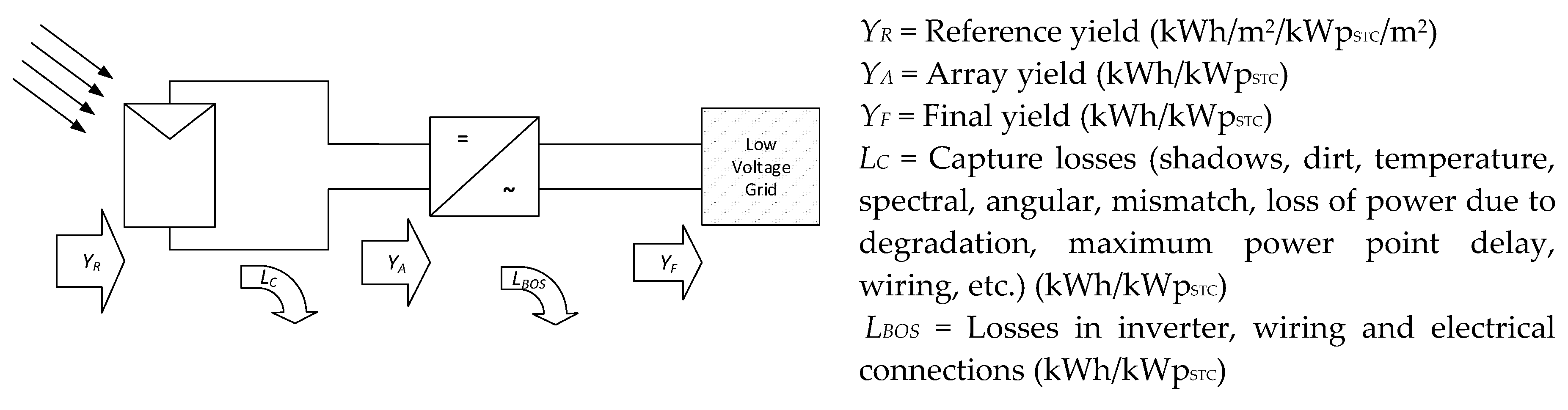
5. Operating Availability Factor, Corrected Energy Yield and Performance Ratios

There are multiple causes of lack of availability in a photovoltaic system and in some cases only a part of the system will be affected, for example, disconnection of a string of modules, while in others there can be total system shutdown caused by tripping of AC protections, absence of network, etc. In order to consider PR and availability independently, a new value of Y R * is defined which only takes into account solar irradiation when the AC power at the inverter output is different from zero. This Y R * (Equation (11)) allows the definition of new energy parameters of the photovoltaic subsystems L C * , P R D C * and P R A C * (Equations (12)–(14)) and availability index (D) (Equation (15)) that eliminate the influence of the difference in the startup and stopping of the inverters and the penalties for faults outside the photovoltaics array, inverters and power grid. These new parameters are exclusively associated with the photovoltaic generator and inverter efficiencies. The availability losses affected only to L C * , P R D C * and P R A C * while that the values of YF, YA and LBOS remain the same as Section 4.
Y R * = T r T G I * G I , S T C = H I * G I , S T C
where G I * and H I * are the global solar irradiance (W/m2) and the global solar radiation (Wh/m2) respectively on the plane of the photovoltaic generator over a period of time T for alternating power above zero.
L C * = Y R * Y A
P R D C * ( % ) = Y A Y R * × 100
P R A C * ( % ) = Y F Y R * × 100
D ( % ) = Y R * Y R × 100
The new values of the production and loss indexes are shown in the Table 9 and Table 10.
How the values of P R D C * and P R A C * have increased with respect to those initially calculated can be seen. The D factor of all the subsystems has remained high in the years 2013 and 2014. In the year 2015 it has fallen ~3% in all the subsystems due to power cuts of the general network, outside the photovoltaic system, except in the subsystem 4 that has more downtime. CdTe/CdS technology continues to have the greatest decrease in the value of P R A C * of 15.5%, ending with 56.2% in 2015. The CIS technology continues to have the highest P R A C * value, with 81.9% in 2015.
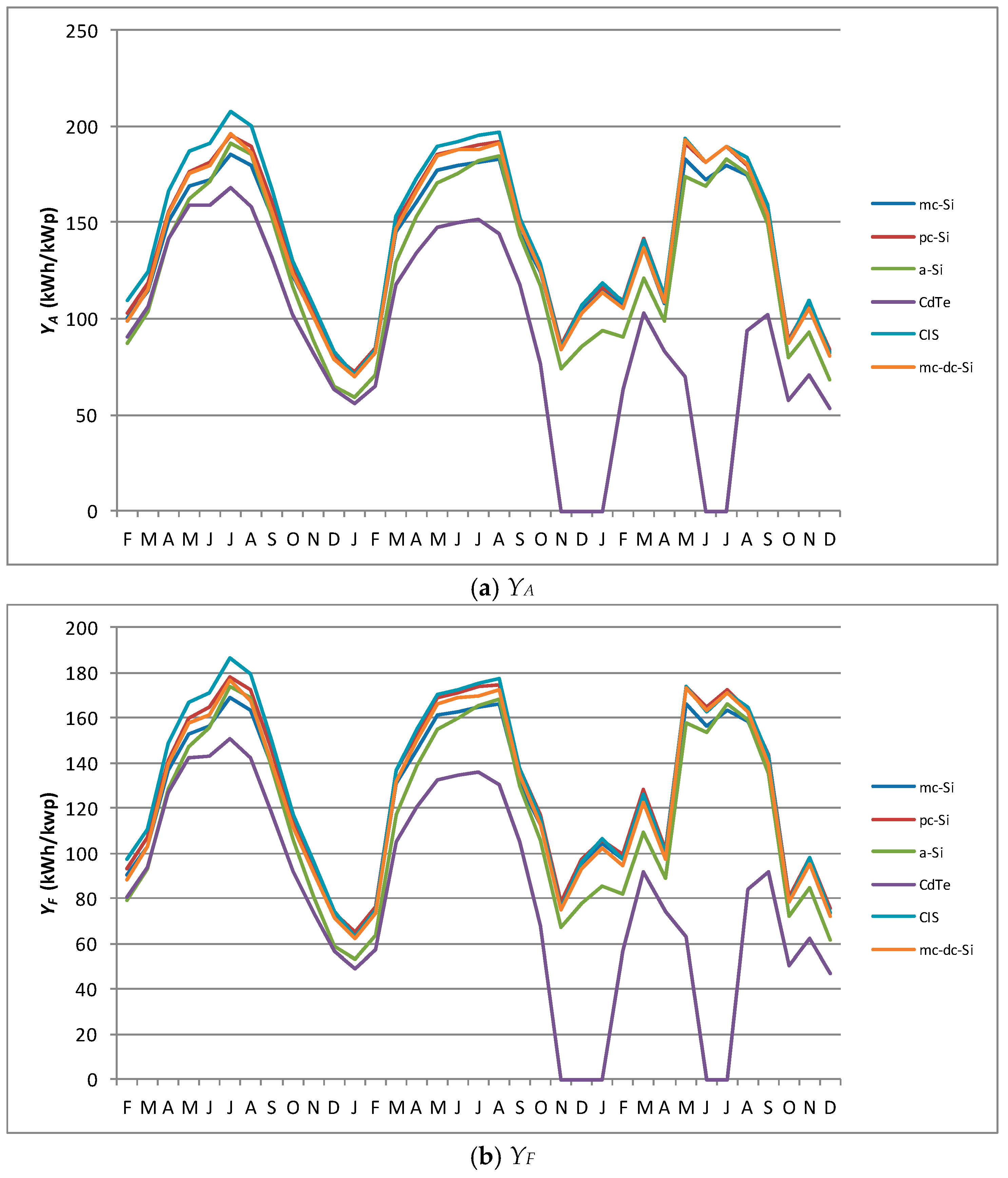
 Figure 13 and Figure 14 show the mean values corresponding to three years of Y R * , YA, YF, L C * , LBOS, P R D C * , P R A C * and factor D.
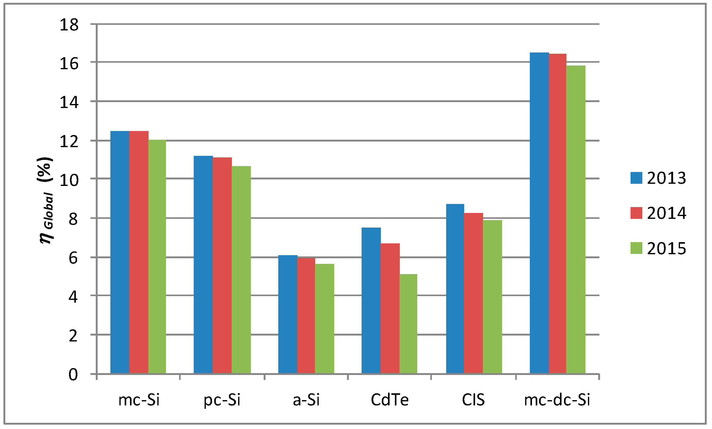
The corrected annual operational efficiency ( η G * ) and aggregated loss of efficiency in the three years studied (Δ η G * ) of the photovoltaic array of each technology has been calculated (Equation (16)) again from this new scenario (Table 11).
η G * ( % ) = E D C H I * · A × 100
The annual loss of efficiency in all technologies are very similar to the values obtained in studies carried out with the same technologies in other locations [41,42,43,44]. 
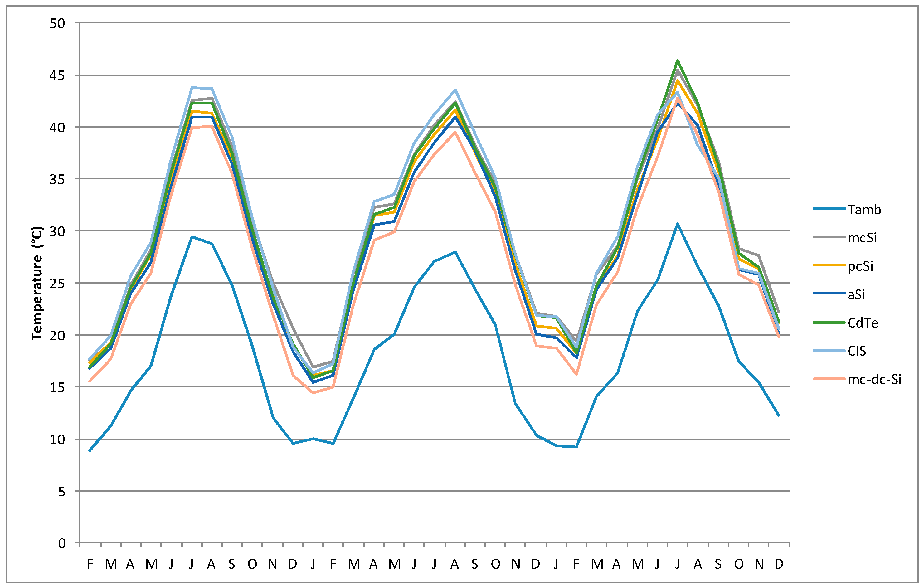
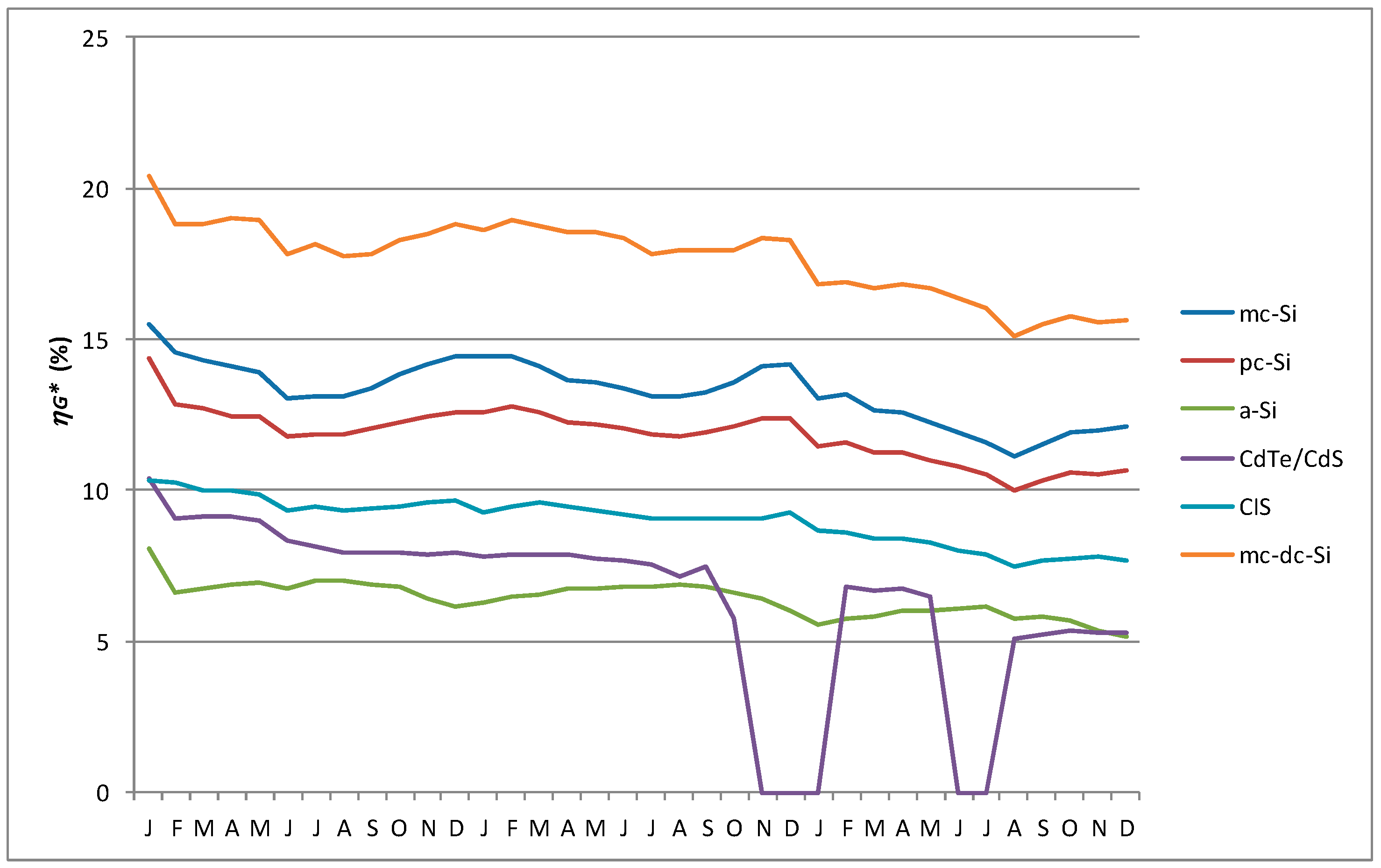
Figure 15 shows the evolution of the monthly-corrected operational efficiency of all technologies. In the first month of solar exposure, February 2013, there is a significant loss of efficiency in all technologies with respect to the values provided by the vendor under STC conditions, except in CIS technology, being 0.8% mc-Si, 1.50% pc-Si, 1.4% a-Si/µc-Si, 1.1% CdTe/CdS, −0.1% CIS and 1.3% mc-dc-Si. Figure 14 shows the annual operational efficiency losses. The technologies pc-Si and CdTe/CdS reduced 1.9% and 1.8% respectively in the first year with CIS technology losing only 0.4%. This annual efficiency loss has been lower in the years 2014 and 2015 as can be seen in Figure 16.
Table 12 provides a summary of the study. The percentage variations of the loss of efficiency in the first month, the first year and the study period are shown with respect nominal efficiency STC of each photovoltaic technology. Also included are the percentage changes in global efficiency and energy production indexes P R A C * and P R D C * .
The efficiency losses in the first month are similar in all technologies except mc-Si that presents minor losses and CIS which has a slightly positive balance positive due to the increase in efficiency during the first hours of sun exposure. The trend continues throughout the first year except for the a-Si/µc-Si technology which has a small yearly increase resulting in a reduction of efficiency loss compared to the first month. The variations in photovoltaic efficiency over the study period is similar for the crystalline silicon technologies, with a-Si/µc-Si showing intermediate values while CdTe/CdS and CIS are at the highest and lowest end of the spectrum respectively. Moreover, CdTe/CdS displays the largest decrease of the global efficiency. Regarding the variations of the P R D C * and P R A C * , CdTe/CdS and CIS are highest while the rest of the technologies are very similar.

6. Conclusions

A photovoltaic installation on the rooftop of the university campus has permitted a comparative study of the energy production rates of six selected photovoltaic technologies connected to the internal electricity network of the university using the same model of inverter under the same physical and climatic conditions, over a period of three years with the following conclusions. The solar irradiation measurements over the study period present small variations with respect to the average meteorological year. The ambient temperature has followed the usual pattern of local climate. The influence of the wind speed can be considered of little relevance. The use of the availability index allows the energy comparative analysis of the technologies for the photovoltaic generator and inverter efficiencies.
The mc-Si, pc-Si, CIS and mc-cd-Si technologies reach an average value of P R A C * above 80%, and a-Si/µc-Si and CdTe/CdS remain at 74.5% and 64.3%, respectively. The loss of efficiency in all technologies during the first month is evident, except for the CIS technology because it initially achieves a gain in efficiency.
The conventional technologies mc-Si and pc-Si displayed very similar thermal and energy behavior. The decrease in the P R D C * and P R A C * values during the three years were lower than for the other technologies, which indicates a more stable behavior, being the values of the pc-Si technology, which had a corrected capture loss of 9%, the highest, while for mc-Si technology it was 12.4%, despite having suffered a major power degradation during the first month.
With respect to thin-film technologies, CIS technology (subsystem 5), is the one that reaches a higher temperature in the summer months. The losses in CIS technology, P R A C * value and global efficiency performance in the three years were 6.3% and 0.79%, respectively, and the generator efficiency loss was 1.3%. Its initial degradation during the first year (0.4%) was the lowest. The mean values of P R D C * and P R A C * during the three years are the highest, with 94.5% and 84.6%, respectively. The corrected capture losses have been the lowest of all technologies at around 6%.
The behavior of the a-Si/µc-Si tandem technology obtains better P R A C * value results during the summer months than the other technologies, having a coefficient of loss of power with the low temperature, confirming it is a more appropriate technology for warm climates. Moreover, the loss of efficiency of the generator in the first year and over the entire number of years has been the lowest, with the exception of CIS technology. The average value of P R A C * is 74.5% and its corrected capture losses reach 20.6%.
CdTe/CdS technology is the one that has had the worst performance. Its loss of efficiency in the first year was similar to that of the pc-Si technology, but during the following two years it suffered a degradation of 2%. Mean values of P R D C * and P R A C * during the three years are the lowest of all technologies, with 72% and 64.3%, respectively. Its corrected capture losses reach a value of 28.6%. This behavior and degradation has been confirmed in previous studies.
The high-efficiency mc-dc-Si technology has an initial loss of efficiency similar to those of the mc-Si and pc-Si technologies. The module operating temperature during the summer months is the lowest out of all technologies. It is the most efficient technology in STC conditions, which translates into the greater value of overall efficiency, but its decrease during the investigation period was 0.8% higher than mc-Si and pc-Si, with 0.53% and 0.54%, respectively. The average P R A C * and corrected capture losses were 80.6% and 10.5%, respectively.
This study expands the performance database of the principal photovoltaic technologies for middle latitude continental climates over an extended period of time, thus enriching the data available to calculate energy produced in the long term, key for determining the Levelized Cost of Energy (LCOE) [91] and the Energy Payback Time (EPBT) [92] of photovoltaic systems.
The study concentrates on side-by-side comparisons and analysis between different commercial PV technologies in the same urban location in Madrid (Spain). The emphasis is placed on the operational availability of each of the platforms as seen by the use of the corrected performance ratio values, permitting an in depth exhaustive study of the concerned technologies. The results obtained add to the body of photovoltaic performance data available worldwide.

Acknowledgments

The authors appreciate the support of the companies AS SOLAR IBÉRICA and SMA Solar Technology AG.

Author Contributions

Teodoro Adrada Guerra elaborated the state of the art of the study, including all calculations, graphs analysis and conclusions. Julio Amador Guerra directed the research work. Beatriz Orfao Tabernero performed the quality control of the monitored data and the preliminary calculations of the energy parameters. These tasks were carried out in the framework of her work toward a Master in Renewable Energies and the Environment degree at UPM, under the mentorship of Teodoro Adrada Guerra and Julio Amador Guerra. Guillermo de la Cruz García collaborated in the design of the photovoltaic and monitoring system. He directed its deployment commissioning, and coordinated the operation and maintenance, solving all the incidences of the data acquisition system.

Conflicts of Interest

The authors declare no conflict of interest.

References

  1. Caamaño, E. Photovoltaic Buildings Connected to the Electricity Grid: Characterization and Analysis. Ph.D. Thesis, Universidad Politécnica de Madrid, Madrid, Spain, 1998. [Google Scholar]
  2. Masa, D. Contribution to the Integration of Grid-Connected Photovoltaic Systems: Solar Resource and Energy Prediction. Ph.D. Thesis, Universidad Politécnica de Madrid, Madrid, Spain, 2014. [Google Scholar]
  3. Makrides, G.; Zinsser, B.; Georghiou, G.; Werner, J. Performance assessment of different photovoltaic systems under identical field conditions of high irradiation. In Proceedings of the Renewable Energy Sources & Energy Efficiency, Nicosia, Cyprus, 28–30 September 2007. [Google Scholar]
  4. Zinsser, B.; Makrides, G.; Schmitt, W.; Georghiou, G.; Werner, J. Annual energy yield of 13 photovoltaic technologies in Germany and in Cyprus. In Proceedings of the 22th European Photovoltaic Solar Energy Conference, Milano, Italy, 3–7 September 2007. [Google Scholar]
  5. Abella, M.A.; Chenlo, F. Estimation of the energy generated by a grid-connected photovoltaic system. ERA Sol. 2006, 131, 36–67. [Google Scholar]
  6. Lorenzo, E. The electricity produced by photovoltaic systems connected to the grid. ERA Sol. 2002, 107, 22–28. [Google Scholar]
  7. Woyte, A.; Richter, M.; Moser, D.; Mau, S.; Reich, N.; Jahn, U. Analytical Monitoring of Grid-Connected Photovoltaic Systems—Good Practices for Monitoring and Performance Analysis; International Energy Agency (IEA): Paris, France, 2014; p. 90. [Google Scholar]
  8. Sidrach-de-Cardona, M.; Mora, L.I. Performance analysis of a grid-connected photovoltaic system. Energy 1999, 24, 93–102. [Google Scholar] [CrossRef]
  9. PVSYST 3.2. Software for the Simulation of Photovoltaic Systems. Available online: http://www.pvsyst.com (accessed on 1 June 2017).
  10. PV Performance Modeling Collaborative PVPMC. Available online: https://pvpmc.sandia.gov/ (accessed on 1 June 2017).
  11. Performance Calculator for Grid-Connected PV Systems. Available online: http://rredc.nrel.gov/solar/codes_algs/PVWATTS/ (accessed on 1 June 2017).
  12. SISIFO Software for the Simulation of Photovoltaic Systems. Available online: http://www.etsit.upm.es/ (accessed on 1 June 2017).
  13. PVValue. Sandia National Laboratories. Available online: http://energy.sandia.gov/ (accessed on 1 June 2017).
  14. HOMER Energy. National Renewable Energy Lab. Available online: http://www.homerenergy.com/ (accessed on 1 June 2017).
  15. RetScreen. National Resources Canada. Available online: http://www.nrcan.gc.ca/ (accessed on 1 June 2017).
  16. PV*SOL Software for Sizing and Design of Photovoltaic Systems. Available online: http://www.valentin-software.com (accessed on 1 June 2017).
  17. SOLAR PRO. Available online: http://www.laplacesolar.com (accessed on 1 June 2017).
  18. Muñoz, J.; Perpiñan, O. A simple model for the prediction of yearly energy yields for grid-connected PV systems starting from monthly meteorological data. Renew. Energy 2016, 97, 680–688. [Google Scholar] [CrossRef]
  19. Perpiñan, O.; Lorenzo, E.; Castro, M.A. On the calculation of energy produced by a PV grid connected systems. Prog. Photovolt. 2007, 15, 265–274. [Google Scholar] [CrossRef]
  20. Chouder, A.; Silvestre, S.; Sadaoui, N.; Rahamani, L. Modeling and simulation of a grid connected PV system based on the evaluation of main PV module parameters. Elsevier Simul. Model. Pract. Theory 2012, 20, 46–58. [Google Scholar] [CrossRef]
  21. Chiou-Jye, H.; Ting, M.; Chung-Cheng, C. A novel power output for photovoltaic systems. Int. J. Smart Grid Clean Energy 2012, 2, 139–147. [Google Scholar]
  22. Chiou-Jye, H.; Chao-Yang, H.; Po-Chun, H.; Shun-Hung, T. A technique for accurate energy yields prediction of photovoltaic system. Int. J. Smart Grid Clean Energy 2013, 3, 51–56. [Google Scholar]
  23. Cherfa, F.; Arab, H.; Oussaid, R.; Abdeladim, K.; Bouchkor, S. Performance analysis of the mini-grid connected photovoltaic system at Algiers. Energy Procedia 2015, 83, 226–236. [Google Scholar] [CrossRef]
  24. Ransome, S. How well do PV Modeling Algorithms really predict performance? In Proceedings of the 22th European Photovoltaic Solar Energy Conference, Milan, Italy, 3–7 September 2007. [Google Scholar]
  25. Chicco, G.; Cocina, V.; Di Leo, P.; Spertino, F.; Massi Pavan, A. Error assessment of solar irradiance forecasts and AC power from energy conversion model in grid-connected photovoltaic systems. Energies 2016, 9, 8. [Google Scholar] [CrossRef]
  26. AEMET. Agencia Española de Meteorología. Available online: http://www.aemet.es/es/portada (accessed on 1 June 2017).
  27. Scharmer, K.; Greif, J. The European Solar Radiation Atlas. Available online: http://www.helioclim.net/esra/index.html (accessed on 1 June 2017).
  28. Solar Radiation Data Obtained by Satellite. Available online: http://eosweb.larc.nasa.gov/sse/ (accessed on 1 June 2017).
  29. METEONORM. Available online: http://www.meteonorm.com/ (accessed on 1 June 2017).
  30. Photovoltaic Geographical Information System. Available online: http://re.jrc.ec.europa.eu/pvgis/ (accessed on 1 June 2017).
  31. HELIOS. Available online: http://helios.ies-def.upm.es/ (accessed on 1 June 2017).
  32. Solar GIS. Available online: http://solargis.info/index.html (accessed on 1 June 2017).
  33. PV Design Pro. Maui Solar Energy Software Corporation. Available online: http://www.mauisolarsoftware.com (accessed on 1 June 2017).
  34. Labed, S.; Lorenzo, E. The impact of solar radiation variability and data discrepancies in the design of PV systems. Renew. Energy 2004, 29, 1007–1022. [Google Scholar] [CrossRef]
  35. Marion, B.; Kroposki, B.; Emergy, K.; Del Cueto, J.; Myers, D.; Osterwald, C. Validation of A Photovoltaic Module Energy Ratings Procedure at NREL. Available online: https://digital.library.unt.edu/ark:/67531/metadc620593/m2/1/high_res_d/12187.pdf (accessed on 1 June 2017).
  36. Gay, C.F.; Rumberg, J.E.; Wilson, J.H. AM-PM: All day module performance measurements. In Proceedings of the 16th IEEE Photovoltaic Specialist Conference, San Diego, CA, USA, 27–30 September 1982; pp. 1041–1046. [Google Scholar]
  37. De Soto, W.; Klein, S.A.; Beckman, W.A. Improvement and validation of a model for photovoltaic array performance. Sol. Energy 2006, 80, 78–88. [Google Scholar] [CrossRef]
  38. Hunter, A.; Davis, M.; Dougherty, B.; King, D.L. Comparison of Photovoltaic Module Performance Measurements. J. Sol. Energy Eng. 2006, 128, 152–159. [Google Scholar] [CrossRef]
  39. Photovoltaic (PV) Module Performance Testing and Energy Rating—Part 1: Irradiance and Temperature Performance Measurements and Power Rating. Available online: https://webstore.iec.ch/preview/info_iec61853-1%7bed1.0%7db.pdf (accessed on 1 June 2017).
  40. Kaldellis, J.; Kapsali, M.; Kavadias, K. Temperature and wind speed impact on the efficiency of PV installations: Experience obtained from outdoor measurements in Greece. Renew. Energy 2014, 66, 612–734. [Google Scholar] [CrossRef]
  41. Makrides, G.; Zinsser, B.; Phinikarides, A.; Schubert, M.; Georghiou, G. Temperature and thermal annealing effects on different photovoltaic technologies. Renew. Energy 2012, 43, 407–417. [Google Scholar] [CrossRef]
  42. Sharma, V.; Kumar, A.; Sastry, O.; Chandel, S. Performance assessment of different solar photovoltaic technologies under similar outdoor conditions. Energy 2013, 58, 511–518. [Google Scholar] [CrossRef]
  43. Cañete, C.; Carretero, J.; Sidrach de Carcona, M. Energy performance of different photovoltaic module technologies under outdoor conditions. Energy 2014, 65, 295–302. [Google Scholar] [CrossRef]
  44. Carr, A.; Pryor, T. A comparison of the performance of different PV module types in temperate climates. Sol. Energy 2004, 76, 285–294. [Google Scholar] [CrossRef]
  45. Carigiet, F.; Baumgartner, F.; Sutterlueti, J.; Allet, N. Energy rating based on thermal modeling of five different PV technologies. In Proceedings of the 29th European Photovoltaic Solar Energy Conference, Amsterdam, The Netherlands, 22–26 September 2014. [Google Scholar]
  46. Schwingshackl, C.; Petitta, M.; Wagner, J.E.; Belluardo, G.; Moser, D.; Castelli, M.; Tetzlaff, A. Wind effect on PV module temperature: Analysis of different techniques for an accurate estimation. Energy Procedia 2013, 40, 77–86. [Google Scholar] [CrossRef]
  47. Gottschalg, R.; Betts, T.R.; Eeles, A.; Williams, S.R.; Zhu, J. Influences on the energy delivery of film photovoltaic modules. Sol. Energy Mater. Sol. Cells 2013, 119, 169–180. [Google Scholar] [CrossRef]
  48. Skoplaki, E.; Boudouvis, A.G.; Palyvos, J.A. A simple correlation for the operating temperature of photovoltaic modules of arbitrary mounting. Sol. Energy Mater. Sol. Cells 2008, 92, 1393–1402. [Google Scholar] [CrossRef]
  49. Alonso, M.; Chenlo, F.; Nofuentes, G.; Torres, M. Analysis of spectral effects on the energy yield of different PV (photovoltaic) technologies: The case of four specific sites. Energy 2014, 67, 435–443. [Google Scholar] [CrossRef]
  50. Dirnberger, D.; Müller, B.; Reise, C. On the uncertainty of energetic impact on the yield of different PV technologies due to varying spectral irradiance. Sol. Energy 2015, 111, 82–96. [Google Scholar] [CrossRef]
  51. Dirnberger, D.; Blackburn, G.; Müller, B.; Reise, C. On the impact of solar irradiance on the yield of different PV technologies. Sol. Energy Mater. Sol. Cells 2015, 132, 431–442. [Google Scholar] [CrossRef]
  52. Tamizhmani, G.; Dignard-Bailey, L.; Thevenard, D.; Howell, G. Influence of Low Light Module Performance on the Energy Production of Canadian Grid-Connected PV Systems; Natural Resources Canada: Ottawa, ON, Canada, 1998. [Google Scholar]
  53. Nofuentes, G.; De la Casa, J.; Torres, M.; Alonso, M. Solar spectral and module temperature influence on the outdoor performance of thin film PV modules deployed on a sunny inlands site. Int. J. Photoenergy 2013, 2013, 620127. [Google Scholar] [CrossRef]
  54. Martin, N.; Ruiz, J.M. Calculation of the PV modules angular losses under field conditions by means of an analytical model. Sol. Energy Mater. Sol. Cells 2001, 70, 25–38. [Google Scholar] [CrossRef]
  55. Martin, N.; Ruiz, J.M. A new method for the spectral characterization of PV modules. Prog. Photovolt. Res. Appl. 1999, 7, 299–310. [Google Scholar] [CrossRef]
  56. Spertino, F.; Corona, F.; Di Leo, P. Limits of advisability for master-slave configuration of DC-AC converters in photovoltaic systems. IEEE J. Photovolt. 2012, 2, 547–554. [Google Scholar] [CrossRef]
  57. Dubewar, S.W.; Patil, D.R. Comparative study of photovoltaic array maximum power point tracking techniques. Int. J. Eng. Res. Technol. 2015, 4, 216–223. [Google Scholar]
  58. Faranda, R.; Leva, S. Energy comparison of MPPT techniques for PV Systems. Trans. Power Syst. 2008, 3, 446–455. [Google Scholar]
  59. Muñoz, J.; Martínez, F.; Lorenzo, E. On site characterization and energy efficiency of grid connected PV inverters. Prog. Photovolt. Res. Appl. 2011, 19, 192–201. [Google Scholar] [CrossRef]
  60. Ndiaye, A.; Kébé, C.M.F.; Chaki, A.; Ndiaye, P.; Sambou, V.; Kobi, A. Degradation evaluation of crystalline-silicon photovoltaic modules after a few operation years in a tropical environment. Sol. Energy 2014, 103, 70–77. [Google Scholar] [CrossRef]
  61. Makrides, G.; Zinsser, B.; Schubert, M.; Georghiou, G.E. Performance loss rate of twelve photovoltaic technologies under field conditions using statistical techniques. Sol. Energy 2014, 103, 28–42. [Google Scholar] [CrossRef]
  62. Raugei, M.; Bargigli, S.; Ulgiati, S. Life cycle assessment and energy pay-back time of advanced photovoltaic modules: CdTe and CIS compared to poly-Si. Energy 2007, 32, 1310–1318. [Google Scholar] [CrossRef]
  63. Chaichan, M.; Mohammed, B.; Kazem, H. Effect of pollution and cleaning on photovoltaic performance based on experimental study. Int. J. Sci. Eng. Res. 2015, 6, 594–601. [Google Scholar]
  64. Del Cueto, J. Comparison of energy production and performance from flat plate photovoltaic module technologies deployed at fixed tilt. In Proceedings of the 29th IEEE Photovoltaic Specialists Conference, New Orleans, LA, USA, 19–24 May 2002. [Google Scholar]
  65. Søndenå, R. Boron-Oxygen-Related Degradation in Multicrystalline Silicon Wafers. Available online: www.pv-tech.org (accessed on 1 June 2017).
  66. Sopori, B.; Basnyat, P.; Shet, S.; Mehta, V.; Binns, J.; Appel, J. Understanding light-induced degradation of c-Si solar cells. In Proceedings of the 38th IEEE Photovoltaic Specialists Conference (PVSC), Austin, TX, USA, 3–8 June 2012. [Google Scholar]
  67. Comparative Study of ILB-ENSOL Modules at Difference Irradiation and Temperature Range. Available online: www.ilbhelios.com (accessed on 1 June 2017).
  68. Characterization of Performance of Thin-film Photovoltaic Technologies. Available online: http://repository.supsi.ch/5776/ (accessed on 1 June 2017).
  69. Ruther, R.; Del Cueto, J.; Tamizh-Mani, G.; Roedern, B. Performance test of amorphous silicon modules in different climates-year four: Progress in understanding exposure history stabilization effects. In Proceedings of the 33th IEEE Photovoltaic Specialists Conference, San Diego, CA, USA, 11–16 May 2008; pp. 1–5. [Google Scholar]
  70. Akhmad, K.; Kitamura, A.; Yamamoto, F.; Okamoto, H.; Takamura, H.; Hamakawa, Y. Outdoor performance of amorphous silicon and polycrystalline silicon PV modules. Sol. Energy Mater. Sol. Cells 1997, 46, 209–218. [Google Scholar] [CrossRef]
  71. Krauter, S.; Grunow, P.; Lehmann, S. The real challenges for photovoltaic modules. In Proceedings of the 25th Anniversary of PASAN, Neuchatel, Switzerland, 12 June 2009. [Google Scholar]
  72. Mohring, H. Optimized procedures for characterization of module energy field. In Proceedings of the Integrated Project Performance Final Forum, European Commission, Malaga, Spain, 11 December 2009. [Google Scholar]
  73. Rose, D.; Koehler, O.; Bourne, B.; Kavulak, D.; Nelson, L. High-confidence prediction of energy production from high-efficiency photovoltaic systems. In Proceedings of the 25th Photovoltaic Solar Energy Conference, Valencia, Spain, 6–10 September 2010. [Google Scholar]
  74. Poissant, Y.; Couture, L.; Dignard-Baley, L.; Thevenard, D.; Cusack, P.; Oberholzer, H. Simple test methods for evaluating the energy rating of PV modules under various environmental conditions. In Proceedings of the ISES Solar World Congress, Göteborg, Sweden, 14–19 June 2003. [Google Scholar]
  75. Gostein, M.; Dunn, L. Light soaking effects on photovoltaic modules: Overview and literature review. In Proceedings of the 37th IEEE Photovoltaic Specialists Conference (PVSC), Seattle, WA, USA, 19–24 June 2011. [Google Scholar]
  76. Willett, D.; Kuriyagawa, S. The effects of sweep rate, voltage bias and light soaking on the measurement of CIS-based solar cells characteristics. In Proceedings of the 23th IEEE Photovoltaic Specialists Conference, Louisville, KY, USA, 10–14 May 1993; pp. 495–500. [Google Scholar]
  77. Deline, C.; Del Cueto, J.; Albin, D.S.; Petersen, C.; Tyler, L.; TamizihMani, G. Transient response of cadmium telluride modules to light exposure. In Proceedings of the 37th IEEE Photovoltaic Specialists Conference (PVSC), Seattle, WA, USA, 19–24 June 2011. [Google Scholar]
  78. Rodziewicz, T.; Pietruszko, S.; Zaremba, A.; Wacławek, M. Long term analysis of energy gained by different PV modules in 2001–2006. In Proceedings of the 22th European Photovoltaic Solar Energy Conference, Milan, Italy, 3–7 September 2007. [Google Scholar]
  79. Baumgartner, F. Euro real inverter efficiency: DC voltage dependency. In Proceedings of the 20th European Photovoltaic Solar Energy Conference, Barcelona, Spain, 6–10 June 2005; pp. 2257–2260. [Google Scholar]
  80. Baumgartner, F.; Schmidt, H.; Bründlinger, R.; Burger, B.; Zehner, M. Status and relevance of the DC voltage dependency of the inverter efficiency. In Proceedings of the 20th European Photovoltaic Solar Energy Conference, Barcelona, Spain, 3–7 September 2007; pp. 2499–2505. [Google Scholar]
  81. Haeberlin, H.; Borgna, L.; Kaempfer, M.; Zwahle, U. News test at grid-connected PV inverters; overview over test results and measured values of total efficiency ηtot. In Proceedings of the 21th European Photovoltaic Solar Energy Conference, Dresden, Germany, 4–8 September 2006; pp. 2272–2275. [Google Scholar]
  82. Jahn, U.; Nasse, W. Performance analysis and reliability of grid-connected PV systems in IEA countries. In Proceedings of the 3rd World Conference on Photovoltaic Energy Conversion, Osaka, Japan, 11–18 May 2003. [Google Scholar]
  83. Photovoltaic System Performance Monitoring-Guidelines for Measurement, Data Exchange and Analysis. Available online: http://www.standardsbis.in/Gemini/scoperef/SRIE61724.pdf (accessed on 1 June 2017).
  84. Blaesser, G.; Munro, D. Guidelines for the Assessment of Photovoltaic Plants Document A Photovoltaic Systems Monitoring; Commission of the European Communities, Joint Research Centre: Ispra, Italy, 1995. [Google Scholar]
  85. Blaesser, G.; Munro, D. Guidelines for the Assessment of Photovoltaic Plants Document B Analysis and Presentation of Monitoring Data; Commission of the European Communities, Joint Research Centre: Ispra, Italy, 1995. [Google Scholar]
  86. Woyte, A.; Richter, M.; Moser, D.; Mau, S.; Reich, N.; Jahn, U. Monitoring of photovoltaic systems: Good practices and systematic analysis. In Proceedings of the 28th European PV Solar Energy Conference, Paris, France, 30 September–4 October 2013. [Google Scholar]
  87. CONERSA. Available online: www.conersa.com (accessed on 1 June 2017).
  88. Spertino, F.; Di Leo, P.; Cocina, V. Accurate measurements of solar irradiance for evaluation of photovoltaic power profiles. In Proceedings of the 2013 IEEE Grenoble PowerTech (POWERTECH), Grenoble, France, 16–20 June 2013. [Google Scholar]
  89. Koehl, M.; Heck, M.; Wiesmeier, S.; Wirth, J. Modeling of the nominal operating cell temperature based on outdoor weathering. Sol. Energy Mater. Sol. Cells 2011, 95, 1638–1646. [Google Scholar] [CrossRef]
  90. Jahn, U.; Nasse, W.; Nordmann, T.; Clavadetscher, L.; Mayer, D. Achievements of Task 2 of IEA PV Power Systems Programme: Final Results on PV System Performance. Available online: www.task2.org (accessed on 29 May 2017).
  91. Darling, S.; You, F.; Veselka, T.; Velosa, A. Assumptions and the levelized cost of energy for photovoltaics. Energy Environ. Sci. 2011, 4, 3133. [Google Scholar] [CrossRef]
  92. Yue, D.; You, F.; Darling, S. Domestic and overseas manufacturing scenarios of silicon-based photovoltaics: Life cycle energy and environmental comparative analysis. Sol. Energy 2014, 105, 669–678. [Google Scholar] [CrossRef]
Figure 1. PV systems on the rooftop of the ETSIDI-UPM in Madrid.
Energies 10 00772 g001
Figure 2. Measuring sensors placed on the rooftop of the ETSIDI-UPM. (a) Thermohygrometer and anemometer. (b) PIR and CRC installed with a tilt of 30° and azimuth of 19° east.
Energies 10 00772 g002
Figure 3. Monitored electrical and meteorological variables of each of the photovoltaic subsystems.
Energies 10 00772 g003
Figure 4. Evolution of global solar radiation HI (kWh/m2), Years 2013–2015.
Energies 10 00772 g004
Figure 5. Evolution of average ambient and modules temperatures.
Energies 10 00772 g005
Figure 6. Average monthly wind speed.
Energies 10 00772 g006
Figure 7. Energy yields and losses parameters.
Energies 10 00772 g007
Figure 8. Evolution of the index.
Energies 10 00772 g008
Figure 9. Evolution of losses.
Energies 10 00772 g009aEnergies 10 00772 g009b
Figure 10. Monthly evolution PRDC (%).
Energies 10 00772 g010
Figure 11. Monthly evolution PRAC (%).
Energies 10 00772 g011
Figure 12. Global energy efficiency.
Energies 10 00772 g012
Figure 13. Average values 2013–2015 of Y R * , YA, YF, L C * , LBOS.
Energies 10 00772 g013
Figure 14. Average values 2013–2015 of P R D C * and P R A C * , D.
Energies 10 00772 g014
Figure 15. Evolution of the operating PV generators efficiency.
Energies 10 00772 g015
Figure 16. Annual operating efficiency loss.
Energies 10 00772 g016
Table 1. Technical parameters of photovoltaic modules.
Technical Parametersmc-Sipc-Sia-Si/µc-SiCdTe/CdsCISmc-dc-Si
Power output STC (WpSTC)25022011577.573333
Power output tolerances (%)0 + 3±3±10±10-5/+8+5/0
Voltage at Pmax (Vmpp 1) (V)29.929.023846.733.954.7
Current at Pmax (Impp) (A)8.377.590.8101.682.216.09
Open circuit voltage (Voc) (V)37.136.517462.543.165.3
Short circuit current (Isc) (A)8.768.150.6611.982.406.46
Module efficiency STC (%)15.514.48.110.410.320.4
αIsc (%/K)0.00430.060.070.020.050.054
βVoc (%/K)−0.338−0.37−0.30−0.24−0.29−0.27
γPmpp (%/K)−0.469−0.45−0.24−0.25−0.36−0.38
NOC temperature (°C)43.7 ± 246 ± 24440 ± 247 ± 345 ± 2
1 mpp = maximum power point.
Table 2. Photovoltaic subsystems.
SubsystemTechnologyYear of ManufactureString ModulesParallel ModulesPower Subsystem STC (WpSTC)Power Subsystem Flash List (WpSTC)Size (m2)
1mc-Si20125112501255.18
2pc-Si20095111001122.28.2
3a-Si/µc-Si200911011501358.614.2
4CdTe/Cds201052775777.67.2
5CIS20088211751176.111.7
6mc-dc-Si20124113321350.66.5
Table 3. Inverter characteristics.
InverterSMA Sunny Boy-1200
Maximum power DC1320 W
Maximum current DC12.6 A
Maximum voltage DC400 V
Voltage range PV (mpp)100–320 V
Nominal output power1200 W
Maximum apparent power1200 VA
Maximum current CA6.1 A
Efficiency92.1%
Table 4. Measuring sensors: manufacturer and specifications.
SensorThermoelectric Pyranometer PIRSensorSolar Cell CRC
Make and modelKipp & Zonen CM3Make and modelATERSA
Spectral range (nm)305–2800Cell typePolycrystalline double cell
Directional error (80° with beam of 1000 W/m2)<±2.5%Relation voltage/radiation100 mV dc = 1000 W/m2
Spectral sensitivity±5% (350–1500 nm)Measurement error ±2.0%
Temperature range−40° to +80°Spectral response300–1100 nm
SensorThermohigrometerAnemometerModular Temperature Sensor
Make and modelWilmers 0535ATERSASTECA PT-1000
Range−30–70 °C
0–100% RH
<0.9–40 m/s−50–180 °C
Measurement error±0.5 °C±5 m/s±0.5 °C
Table 5. Average monthly values of global solar irradiation HI (kWh/m2) and diffuse irradiation fraction (Dh/GI) measured with a tilt of 30° and azimuth of 19° east.
MonthAverage 2013–2015Average Year PVGISAverage 2005–2016 HELIOS
PIRaveCRCavePIRPVGISDh/GIDh/GI
January102.5102.797.60.420.40
February106.2104.6105.20.370.34
March150.0147.0173.20.390.35
April156.8157.9166.20.370.36
May211.6203.2200.20.340.32
June217.7207.7205.50.280.29
July219.5219.8218.80.210.19
August224.1214.7208.30.230.21
September181.0176.1176.70.280.28
October124.4126.5139.50.360.35
November110.2109.196.30.400.37
December96.398.178.70.420.38
Total year1866.21833.21864.7--
Table 6. Annual energy production of each subsystem.
SubsystemPeak Power (WpSTC)Annual Network Production (kWh/Year)
201320142015Total
112501733185618245413
211001589170316694961
311501529161115594699
47759458074902242
511751761181917565336
613321877201119715839
Total year678294349807926928,510
Table 7. Nominal and operational efficiency of the photovoltaic generators.
SubsystemNominal Efficiency STC (%)Operational Efficiency (%)ΔηG (%)
201320142015
115.513.813.713.2−2.3
214.412.312.211.7−2.7
38.16.76.56.2−1.9
410.48.47.45.7−4.7
510.39.79.28.7−1.6
620.418.418.317.6−2.8
Table 8. Average annual efficiency.
Subsystemηinv (%)ηinv, average (%)
201320142015
190.6390.5890.7190.6
290.7690.7090.8590.8
390.5790.4890.6490.6
489.4789.3689.1989.3
589.5289.5289.6889.6
689.9689.8990.0190.0
Table 9. Energy field and losses parameters (kWh/kWpSTC year).
Subsystem201320142015
Y R * YAYF L C * LBOS Y R * YAYF L C * LBOS Y R * YAYF L C * LBOS
11724.801529.41386.3195.41143.01873.01637.71484.6235.3153.11852.91605.61459.2247.2146.4
21721.651591.31444.8130.38146.51873.51704.71547.8168.8156.91851.11657.11517.3193.9139.8
31718.791467.61329.8251.18137.81870.01546.41401.0323.7145.41848.61495.31355.7353.3139.6
41701.831361.71219.4340.14142.31697.41163.01041.7534.3121.41112.4696.0632.8416.463.2
51707.691673.61498.834.09174.81851.31727.61548.1112.1179.51835.51665.91494.516.6171.4
61710.941565.71408.9145.24156.81873.01678.31510.1185.2168.21847.11635.31479.7211.8155.6
Table 10. Comparison between values of PRDC, P R D C * (%) and PRAC, P R A C * (%) and operative availability factor D (%) in three years.
SubsystemYear 2013Year 2014Year 2015
PRDC P R D C * PRAC P R A C * DPRDC P R D C * PRAC P R A C * DPRDC P R D C * PRAC P R A C * D
188.489.679.780.898.687.988.379.680.099.584.487.576.579.296.6
291.793.181.582.798.491.291.682.783.099.586.190.178.180.996.5
383.284.675.376.698.281.381.973.674.199.377.380.370.172.896.4
478.080.269.771.797.169.472.851.765.095.453.96335.656.284.4
596.298.586.188.297.691.993.682.383.898.287.291.378.281.995.5
690.091.879.881.49889.490.380.481.19984.888.776.379.296.4
Table 11. Corrected operational efficiency and cumulative losses of the PV array.
SubsystemNominal Efficiency ηSTC (%)Operational Efficiency η G * (%)Δ η G * (%)
201320142015
115.514.013.813.4−2.1
214.412.512.311.9−2.5
38.16.96.66.4−1.7
410.48.67.86.6−3.8
510.39.99.49.0−1.3
620.418.818.517.9−2.5
Table 12. Percentage changes produced in generators efficiency and performance ratios.
SubsystemTechnologiesEfficiency Degradation (%)Variation
First Month First Year Photovoltaic Efficiency (%) 2013–2015Global Efficiency (%) 2013–2015 P R D C * (%) 2013–2015 P R A C * (%) 2013–2015
1mc-Si−0.8−1.5−2.1-−2.1−1.6
2pc-Si−1.5−1.9−2.5−0.54−3−1.8
3a-Si/µc-Si tandem−1.4−1.2−1.7−0.45−4.3−3.8
4CdTe/CdS−1.1−1.8−3.8−1.8−17.2−15.5
5CIS+0.1−0.4−1.3−0.79−7.2−6.3
6mc-dc-Si−1.3−1.6−2.5−0.8−3.1−2.2

