
Optimal Placement and Sizing of Renewable Distributed Generations and Capacitor Banks into Radial Distribution Systems


1
Department of Electrical and Electronics Engineering, Universiti Teknologi PETRONAS, Seri Iskandar 32610, Perak Darul Ridzuan, Malaysia
2
Department of Electrical Engineering, Mehran University of Engineering and Technology, Jamshoro 76062, Sindh, Pakistan
*
Author to whom correspondence should be addressed.
Energies 2017, 10(6), 811; https://doi.org/10.3390/en10060811
Submission received: 31 January 2017
/
Revised: 9 June 2017
/
Accepted: 11 June 2017
/
Published: 14 June 2017
(This article belongs to the Special Issue Electric Power Systems Research 2017)
Abstract
:In recent years, renewable types of distributed generation in the distribution system have been much appreciated due to their enormous technical and environmental advantages. This paper proposes a methodology for optimal placement and sizing of renewable distributed generation(s) (i.e., wind, solar and biomass) and capacitor banks into a radial distribution system. The intermittency of wind speed and solar irradiance are handled with multi-state modeling using suitable probability distribution functions. The three objective functions, i.e., power loss reduction, voltage stability improvement, and voltage deviation minimization are optimized using advanced Pareto-front non-dominated sorting multi-objective particle swarm optimization method. First a set of non-dominated Pareto-front data are called from the algorithm. Later, a fuzzy decision technique is applied to extract the trade-off solution set. The effectiveness of the proposed methodology is tested on the standard IEEE 33 test system. The overall results reveal that combination of renewable distributed generations and capacitor banks are dominant in power loss reduction, voltage stability and voltage profile improvement.
1. Introduction
Worldwide demand for electricity is increasing. This is due to population growth, urbanization and extensive development of industrial zones. According to the annual energy outlook report [1], the electricity demand in 2040 will reach to 4.93 trillion kWh, which is 28% higher compared to electrical demand in 2011. On the other hand, power companies are facing major challenges in the generation of electrical power and its delivery. The generation of electrical power is mostly through conventional fuels which are detrimental to the environment and its delivery is through transmission lines which are transmitting power at maximum capacity. Hence, the interest of power enterprises are towards utilizing the alternative mean of power generation called renewable power generation or renewable distributed generation (DG). The wind, solar and biomass are the prominent renewable DGs used worldwide for power generation. Italy reports the highest worldwide grid-connected DG of 10 GW via solar PV, and Northwest Ireland shows 307 MW connected via wind DG to its distribution system [2].
The DG in distribution system has many benefits as they are connected near to load centers. It reduces the power flow, minimizes the system losses, increases the voltage profile and strengthens the voltage stability etc. The integration of DG in the distribution system relieves the transmission lines and extends network deferral. Moreover, the integration of DGs also helps in controlling voltage regulation, spinning reserve and network reactive power. However, renewable-based distributed generation i.e., wind and solar have an intermittent nature. The production of this intermittent power generation and load variation introduces many obstacles in the distribution system. These obstacles are voltage rise and dips, power oscillations, voltage stability issues and increase in power losses, so, optimal placement and sizing of renewable DGs and capacitor banks have an overall positive impact.
In last few years, optimal placement and sizing of DG in distribution systems remains a highly researched topic in the power system [3,4]. Most of the authors have proposed methodologies to reduce stressed problems with the assumption that DG modules are dispatchable. In [5,6,7,8,9,10,11,12] the authors used the dispatchable DG type for power loss minimization and voltage profile improvement as a multi-objective problem. The power loss minimization and voltage stability improvement as multi-objective optimization are researched by [13,14], whereas references [15,16,17,18,19] consider the power loss minimization, voltage profile improvement and voltage stability improvement as a multi-objective optimization problem. Different optimization techniques such as the dynamic search algorithm [13], weighted multi-objective index [5], SA [8,12], BAT algorithm [6], adaptive GA [7], CSA [10], PSO [16], MOPSO [9,11,14], QOTLBO [15], improved MOSH [18] and BFA [19] have been considered. References [5,6,20,21,22,23,24,25,26,27,28] used the active and reactive power DG for a multi-objective problem with different optimization algorithms i.e., analytical methods [22,25,28], improved ICA [20], GWO [21], weighted MO [5], COA [23], PSO [24,27], ABC [26] and Bat algorithm [6]. The penetration of renewable power in the distribution system is increasing linearly and the fact is that none of the above authors introduced renewable DG as input. In [29,30,31,32] wind, solar, biomass, fuel cell and micro-turbine type of DGs were used for multi-objective DG placement and sizing problems. However, the output power of wind energy and solar PVs are intermittent in nature, so assuming their output power as dispatchable DG will have an adverse effect on system performance. The intermittency of wind and solar power DG can be mitigated with the help of energy storage [33]. However, the economic viability and recovery of energy storage in the distribution system creates new challenges. Moreover, the probabilistic model with different probability distribution functions (PDFs) is often used to calculate the effective power output as introduced from wind and solar DGs. In [34,35,36,37] the time varying stochastic wind and solar PV module were used for the optimal placement and sizing problem of DG. Among them, [37] considers the probabilistic optimal DG placement problem with the wind, solar and capacitors. Considering the fact, power production from wind speed and solar irradiance are inherently intermittent and smaller compared to distribution load demand.
Hence, this paper proposes a methodology for optimal placement and sizing of the intermittent (i.e., wind turbine and solar PV), non-intermittent (i.e., biomass) renewable DG along with the addition of reactive powers (i.e., capacitor banks) in radial distribution systems. The output of intermittent renewable DGs (i.e., wind turbine and solar PVs) are calculated using multi-state modeling with suitable probability functions. The biomass DG is kept as dispatchable DG, whereas the capacitor banks are modeled in discrete size. An advanced-Pareto-front non-dominated sorting- based multi-objective PSO optimization (advanced-MOPSO) algorithm is proposed for this multi-faceted problem. The convergence speed performance of the proposed algorithm is also modified using a mutation operator. Fast convergence is preferable in any algorithm, but it is feared that it may result in false Pareto-solutions in the context of multi-objective optimization. Therefore, this operator helps in maintaining the particles within the search space. Basically, the mutation operator increases the explorative behaviour for all particles at the start of the algorithm and later its effect ceases gradually. Moreover, the output results of proposed method is not in a single solution rather it gives a Pareto-solution set. Hence, a fuzzy decision technique is implied to find the best trade-off solution among them. The efficiency and performance of proposed method were validated against many single and multi-objective optimization techniques, which were reported in our previous work [38].
The remainder of this paper is organized as follows: Section 2 presents the formulation of generation-load model. Section 3 presents the problem formulation for objective functions and load flow analysis. Section 4 presents the optimization technique i.e., MOPSO, Section 5 analyzes the generation and load model. Section 6 presents the simulation results and discussion. Section 7 presents the performance evaluation of the MOPSO method and Section 8 concludes with a summary of the problem findings.
2. Distributed Generation (DG) Modeling
2.1. Biomass DG Modeling
Biomass DGs is considered as firm supply or constant output power DGs. In other words, fuel inputs to these DGs are constant. Hence, this DG provides rated output power with no uncertainty. Power delivery from this generator can be dispatched according to load curve at a specific time by the distribution network operator.
2.2. Capacitor Bank Modeling
Capacitor banks are devices which produce reactive power [39]. The amount of reactive power produced depends on the size of the capacitors. They are currently available on the market as constant (discrete) type. However, in literature, many authors have supposed them as a continuous variable [40,41,42]. Assuming that a discrete capacitor size with continuous variable may not guarantee a feasible solution, hence, this study considers the discrete size of capacitors for optimal planning of renewable-based DGs in the distribution system. The capacitors available on the market are smaller units (150 KVAr), which are further integer multiples of factor U. Hence, the required amount of capacitor size can be determined using Equation (1) as reported in [43]:
where is an integer. Therefore, the required amount of KVAr can be assessed such as [, 2, 3,…, ].
2.3. Renewable DG Modeling
Different types of renewable DGs are used in the distribution system. Among them, wind speed- and solar irradiance-based renewable DGs are the most dominant and widely interconnected into the radial distribution system. Hence, this paper considers these two renewable DGs, i.e., wind speed- and solar irradiance-based power generation. Accurate wind speed and solar irradiance modeling is quiet challenging. Most of the literature assumes a yearly mean for wind and solar irradiance modeling which generates non-feasible results. Hence, this paper utilizes an hourly multi-state modeling, in a sense that different states of each hour are processed through suitable probability density functions, which guarantee the best output results and perfect stochastic modeling for the wind and solar irradiances. The historical wind speed and solar irradiance data are used to model the wind and solar farms as explained in the following sections.
2.3.1. Wind Speed Modeling
The technology used for converting the kinetic energy of wind to electricity is a wind turbine. Recently, a new development observed in this field has been to increase the output of power generation. In order to extract maximum energy from these wind turbines, peak wind speed areas such as high altitude and sea-side areas are more preferable. In recent years, more and more power generation through wind turbines is being integrated into distribution systems due to its inexhaustible and nonpolluting characteristics. Power generation from wind turbines is fuel free and requires less operational and maintenance cost compared to power generation through conventional means. However, the main drawback of this technology is the intermittency of its output. Wind speed is not constant throughout the day. This results in variations in its power output, which ultimately deteriorates the power quality i.e., increases the rise and dips of voltage profile, power losses and decreases the voltage stability of the power system. Moreover, the stochastic characteristics of wind speed can be modeled in particular time framework using Weibull probability density function as reported in [36,37,44]. The following Equation (2) represents the Weibull distribution for particular wind speed at tth time hour, given as follows:
where is the probability of wind speed at tth time hour. and are the shape and scale parameter respectively. The and of the wind speed can be measured by following Equations (3) and (4):
where and shows the mean and standard deviation of the wind speed at tth time hour. The probability of wind speed at any specific hour for states can be calculated by integrating the probabilities of each state during that hour as given in Equation (5):
2.3.2. Power Generation from Wind Turbines
The power output from wind turbines depends upon the wind velocity available at the site and power curve given from the manufacturer of the wind turbine. Hence, mathematically output power of wind turbine during tth time hour at each state p can be calculated by the following Equation (6):
where is the output power of wind turbine at time hour, is the power output of wind turbine given from the manufacturer at state p can be calculated by Equations (7)–(9) as given below:
where is the characteristics of power generation taken from the power performance curve provided by the manufacturer at each of pth state. is the rated output power from the wind turbine, is the average wind speed, is the cut-in speed, is the rated speed and is the cut-out speed.
2.3.3. Solar Irradiance Modeling
The stochastic characteristics of solar irradiance can be modeled in a particular time framework using Beta probability density function as reported in [45]. The applicability of this model has been employed in a number of solar studies such as [36,37,44]. The following Equations (10)–(12) represent the Beta distribution for particular solar irradiance at tth time as:
where is the Beta distribution function of solar irradiance s at tth time hour, s is the solar irradiance measured in (kW/m2), and are the statistical parameter of and can be calculated by the mean (μ) and standard deviation (σ) of the random variable s as follows:
The probability of solar irradiance at any specific hour for many states can be calculated by integrating the probabilities of each state during that hour as given in Equation (13):
2.3.4. Power Generation from Solar PV
The power output from solar PV modules depends upon the solar irradiance available at the site and PV module characteristics given from the manufacturer. Hence, mathematically output power from solar PV module during tth time hour at each state p can be calculated from the following Equation (14):
where is the output power of solar PV module at time hour, is the power output of solar PV module given from manufacturer at state p can be calculated by Equations (15)–(19) as given below:
where and are the cell temperature and ambient cell temperature during state p, both are measured in (°C). is the mean irradiance of state p. is the nominal operating temperature measured in (°C). and are the total current and voltage of state p, whereas and are the short circuit current measured in (amps) and open circuit voltage measured in (volts). and are the current and voltage temperature coefficient measured in (amps/°C) and (volts/°C) respectively. and are the current and voltage at maximum power point, measured in amps and in volts respectively. N is the total number of PV modules and FF is the fill factor.
2.4. Load Modeling
The proposed test system is assumed to follow the IEEE-RTS load pattern. The time varying load profile values for each hour at typical season is taken from [36].
3. Problem Formulation
The proposed model is designed to integrate intermittent and non-intermittent renewable energy with capacitor banks in a radial distribution system to optimize three objective functions, i.e., power loss reduction, voltage stability improvement and voltage deviation minimization. The distribution system has high resistance to reactance ratio, so the conventional load flow used in transmission line have convergence problem when using it in the distribution system [46,47]. Therefore, this study considers the backward-forward load flow analysis for power flow analysis.
3.1. Power Loss Reduction
It is stated that about 13% of total power generation is wasted as losses in the distribution system [17,19]. Therefore, the first objective of this paper is set to minimize power losses in the radial distribution system. Figure 1 represents the one-line diagram of two buses and connected through branch .
Power loss for the referred distribution system at branch can be computed by the following set of recursive Equations (20)–(22):
where and are the real and reactive powers of the branch . interconnecting bus m1 with , and are the real and reactive loads at bus . and are the voltage magnitudes of the buses and respectively. are the resistance and reactance of the branch i. is the current flowing from to . The power losses across each branch and of the whole system can be computed using Equations (23)–(25):
where and are the real and reactive power losses for the branch respectively, while is the total network loss. This paper considers the active power loss reduction of the network as objective function, which mathematically can be expressed as:
3.2. Voltage Stability Index
Voltage stability index (VSI) is an indicator which shows the stability of distribution system [16,34,35]. This paper is intended to observe the voltage stability of the system with the installation of different types of DGs. Equations (27)–(29) represent the mathematical expression for the voltage stability index as a second objective function. In order to maintain the security and stability of distribution system, the . value should be greater than zero; otherwise the distribution system is under critical instability conditions:
where is the VSI for bus and is the VSI for whole system ; is the total number of buses. In order to improve the voltage stability index, the second objective function can be presented as below:
3.3. Voltage Deviation
The radial nature of distribution system causes voltage dips in heavy load and remote areas. Hence the third objective function for this study is set to minimize the voltage deviation. The mathematical index can be formulated as in the following Equation (30):
3.4. Network Constraints
The Equations (31)–(37) represent the equality and non-equality constraints of the proposed model.
3.4.1. Power Balance
3.4.2. Position of DG
Bus 1 is the substation or slack bus, so the position of the DG should not be used at bus 1:
3.4.3. Voltage Magnitudes
In order to maintain the quality of power supplies, the voltage magnitudes of every bus in the network should satisfy the following constraint:
3.4.4. Boundary Condition of DGs
The boundary condition of the renewable DGs and capacitors are also restricted, which is given as in Equations (35) and (36):
3.4.5. Line Capacity Constraints
The line capacity constraints of line i is limited by its maximum thermal rating limit as:
4. Multi-Objective Optimization (MOO)
Many science and engineering applications are being optimized with meta-heuristic optimization algorithms. In real practice, most of the problems have numerous contradictory objectives which need to optimize simultaneously. Thus, the output of MOO is not in single value but rather forms a pareto optimal set, comprising of several optimal solutions. The non-dominated sorting—based strategy is mostly implied to trade-off the optimal solution set. In general the MOO problem can be formulated as:
where is the function of and is the total number of objective functions. The and are the decision variable and its space respectively and are the constraint functions of the problem, respectively.
4.1. Multi-Objective Particle Swarm Optimization (MOPSO)
The Particle Swarm Optimization (PSO) algorithm was given by Kennedy and Eberhart in 2001. The algorithm is inspired by the natural behavior of birds in flock and fish schooling, which develops their atmosphere to search for food [36]. The conventional or original PSO is simple and computationally efficient but lacks the multi-objective problem handling. Hence, MOPSO is proposed for this study. The MOPSO is an extension of original PSO, given by [48], that is capable of handling many objective functions in one run. The algorithm basically runs in a sense that at every iteration a set of non-dominated solution is recovered, and stored in temporary external repository (REP) file (other than swarm). The REP consists of two main parts, called archive controller and the grid. The function of the former is to decide whether a particular solution should enter into REP or not. Whereas the function of the latter is to produce well-distributed Pareto fronts. Among the REP members, one leader is selected to update the velocity and position of particle . After updating the velocity and position of particles, a new parameter is introduced in the main algorithm, called mutation factor. The mutation factor actually increases the explorative behavior among the particles at the beginning and later it ceases, as number of iteration increases. The pseudocode of the mutation operator is presented in Algorithm 1, below. Moreover, this algorithm gives a set of non-dominated solution set where none of objective function got the superiority in search space or the results are the best compromise pareto-fronts among the whole solution set. Here, fuzzy decision technique is applied to trade-off the solution set. The mathematical formulas for fuzzy decision model are presented in Equations (39) and (40).
| Algorithm 1. Pseudocode for the mutation operator |
| % mu = mutation rate % rr = reducing rate % iter = current iteration % maxiter = maximum iteration % varmax = particle’s upper boundary % varmin = particle’s lower boundary |
| 1: initialize reducing rate (rr) |
| rr = (1-(iter-1)/(maxiter-1))^(1/mu) |
| 2: if rand < rr |
| 3: function mutation_factor (particle, rr, varmax, varmin) |
| 4: Calculate mutation range (m_range) |
| m_range = (varmax-varmin) x rr |
| 5: Assign particle’s upper and lower bounds |
| ub = particle+ m_range lb = particle-m_range |
| 6: Verify particle’s upper and lower bounds |
| if ub > varmax then ub = varmaxif lb < varmin then lb = varmin |
| 7: Assign new values to particle within upper and lower bounds |
| particle = unifrnd (lb,ub) |
| 8: end function |
4.2. Algorithm Implementation
First, initialize the random population for optimal placement size (for biomass DG) and type of DGs (wind, solar and biomass) and capacitor banks. Then, find the fitness function; update the position and velocity of particles at each iteration and find optimal compromise non-dominated pareto-solution set. The main input parameters for the advanced-MOPSO need to be pre-defined, such as shown in Table 1. The complete algorithm is presented in flow chart given in Figure 2 and in following steps:
- Initialization: initialize the population.
- For .
- Initialize .
- Initialize the velocity of each particle.
- Run the load flow and find the fitness function of each hours in all seasons.
- Determine domination among the particles and save the non-dominated particles in repository archive (). The new generated solutions are added to repository and the dominated solutions are removed from repository.
- Update the personal best .
- For .
- Find the leader from .
- In order to select the leader from members of the repository front, firstly the member of repository front is gridded. Then, the roulette wheel technique is used so that cells with lower congestion have more chance to be selected. Finally, one of the selected grid’s members is chosen randomly.
- Uate the speed of each particle using Equation (22).
- Update the new position of each particle using Equations (23)–(25).
- Run the load flow and find the fitness function of each hours in all seasons.
- Apply mutation factor.
- Run the load flow and find the fitness function of each hours in all seasons.
- Add non-dominated solution set of the recent population in the repository.
- Determine the domination among the particles and save the non-dominated particles in repository archive .
- Check the size of the repository. If the repository exceeds the predefined limit, remove the extra members.
- The rest of the members in the repository will be taken for the final solution.
- The optimal compromise solution will be chosen.
5. Wind, Solar and Load Data Analysis
The system inputs include DGs and load. The DGs used in this paper are intermittent (i.e., wind and solar), non-intermittent (i.e., biomass) and capacitor banks. Among them, the wind and solar DGs are dependent on its primary input, wind speed, and solar irradiance. Five years of wind speed and 15 years of solar irradiance data are gathered from the site under survey as for wind speed and for solar irradiance, the probabilistic nature of wind speed and solar irradiance are modeled using Weibull and Beta distribution functions as mentioned above and are further processed with an appropriate time varying model. The time varying model is divided in a sense that 3 months represent a season (i.e., summer, autumn, winter and spring) and each season is set as a day of 24 h. The hourly wind speed and solar irradiance data points have been obtained. Furthermore, in order to extend the robustness in a probabilistic model, the hourly wind speed and solar irradiance are processed through multi-state modeling. For every hour of wind speed and solar irradiance there exist 15 and 20 states, respectively. The probability of every state has been found and from power performance curve of the wind turbine and solar panel, the output power has been measured.
The load demand is also following the hourly time-varying probabilistic model. A day represents the 24 h of one season as mention in Figure 3. The mean and standard deviation of wind speed and solar irradiance of each season are mentioned in Table 2 and Table 3. The multi-state PDF of the wind and solar irradiance for one hour is depicted in Figure 4 and Figure 5. Power output from the wind and solar PV depends upon the characteristics curve of the wind turbine and solar PV.
6. Simulation Results and Discussion
This section provides the optimal placement and sizing of intermittent and non-intermittent renewable energy with capacitor banks for power loss reduction, voltage stability improvement, and voltage deviation minimization. The proposed model is executed using advanced-MOPSO optimization algorithm. The fuzzy decision making method is used to trade-off the solution set. The proposed model is tested on standard 1 MVA, 12.66 KV IEEE 33 radial distribution system. Figure 8 shows the one-line diagram, and its input parameters can be found in Table A1 in the Appendix. The peak active and reactive power load of this test system is 3715 KW and 4300 KVAr respectively. This test system is processed through different seasonal loads which follows the load curve as mentioned in Figure 3. It is a fact that the distribution system is not advanced enough to integrate any amount of DG power. On the other hand, the distribution system is mostly operated in public places. Therefore, this paper suggests four solar farms of 250 kW each having 1000 solar plates, four wind farms each of 250 kW, eight capacitor banks of 125 KVar. The rest of the energy is balanced by 0–2 MW biomass DG. Moreover, the proposed algorithm can integrate any number of renewable DGs and capacitor banks into the distribution system without constraints violation. The 0.95–1.05 p.u voltage magnitude is set to follow as the constraints at each hour. The proposed model is performed on Intel core I5, 4096 MB RAM using MAT-LAB 2015a software package.
After the simulation run, a set of non-dominated solution is recovered from MOPSO algorithm, as presented in Table A2 in the Appendix. It can be observed from the non-dominated solution set results that none of the solutions are unique. Hence, a fuzzy decision model is utilized to select the best trade-off solution. Table 6, presents the optimization results of three objective functions at the base case and after installation of renewable DGs and capacitor banks correspond to obtained non-dominated solution. Table 7, shows the optimal placement and sizing of renewable DG units and capacitor banks in the distribution system. The results for average power losses reduction, minimum average voltage stability index improvement and minimum average voltage deviation before and after installation of renewable DGs and capacitor banks are highlighted in the following sections.
6.1. Power Loss Reduction
A significant amount of power loss reduction has been observed with the integration of renewable DGs with capacitor banks. In summer, the total average power loss before installation of DGs was observed as 148.2 kW, which was reduced to 36 kW (i.e., 75.71%) after installation of DGs. In autumn, the total average power loss was observed as 48.4 kW, which was reduced to 20.5 kW that is 57.64% power loss reduction as compared to total average power loss. In winter, the total average power loss improved to 31.7 kW from 71.4 kW, which represents a 69.61% power loss reduction. Lastly, in spring, the total average power loss was 55.5 kW, which was reduced to 19.9 kW and remained at 64.14%. The power losses of all seasons (i.e., summer, autumn, winter and spring) at each hour, before and after installation of DGs are depicted in Figure 9.
6.2. Voltage Stability Improvement
The integration of renewable DGs with capacitor banks increases the voltage stability index. The index values near to 1.0, represents the good stability of the system. In summer, the minimum average VSI values before installation of DGs was observed as 0.7214 p.u, which improves to 0.8891 p.u (i.e., 23.25%) after installation of DGs. In autumn, the minimum average VSI values were observed as 0.8317 p.u, which improves to 0.9671 p.u, that is 16.28% VSI values as compared to total minimum average VSI values.
In winter, total minimum average VSI values are improved 0.95 p.u from 0.7988 p.u, which calculates to 20.56% VSI values improvement. Lastly in spring, the minimum average VSI values were 0.8207 p.u, which improves to 0.9617 p.u and remained at 17.18%. The VSI values of all seasons at each hour before and after installation of DGs can be observed in Figure 10.
6.3. Voltage Profile Improvement
The integration of renewable DGs with capacitor banks improves the overall voltage profile of the system. In summer, the minimum average voltage profile values before installation of DGs was observed as 0.9212 p.u, which improves to 0.9708 p.u (i.e., 5.38%) after installation of DGs. In autumn, the total minimum average voltage profile values were observed as 0.9549 p.u, which improves to 0.9917 p.u, that is 3.85% voltage profile values as compared to total minimum average voltage profile values. In winter, total minimum average voltage profile values are improved 0.9872 from 0.9452 p.u, which calculates to 4.44% voltage profile values improvement. Lastly in spring, the total minimum average voltage profile values were 0.9903 p.u, which improves to 0.9517 p.u and remained at 4.06%. The voltage profile values of all seasons at each hour before and after installation of DGs can be observed in Figure 11.
7. Performance Evaluation of the MOPSO Method
The efficiency and robustness of non-dominated sorting based multi-objective PSO are checked with many test problems as given in [48]. However, to show the effectiveness of proposed method for optimal integration of distributed generation into the radial distribution system, this paper considers two objective functions i.e., power loss reduction and voltage stability improvement as the test problems. The two i.e., spacing and generational distance metrics are adopted to measure the performance of proposed MOPSO. The detail of spacing and generational distance metrics are specified in [48]. The smaller value of spacing and generational distance witnesses better distribution of solutions and pareto optimal set. In order to perform the simulations, this paper considers the similar algorithm parameters as highlighted in [48] such as population (100 particles), repository size (100 particles), mutation rate (0.5) and 30 adaptive grid division. The results of proposed test problem for these two metrics are obtained and compared with other test problems as given in Table 8 and Table 9.
It can be observed from Table 8 and Table 9 that the results obtained from spacing and generational distance metric for two objective functions problem as suggested are very near to the compared test problems. Hence, it shows that the proposed MOPSO method gives better convergence and Pareto solution to the problem highlighted of this paper. Moreover, the computational time for proposed technique with 200 numbers of iterations, 500 population size and 100 repository size takes 6488.24 s for all seasons and hours. It is worth noting around 6324.42 s are required for load flow calculations, which are performed three times at each hour. Hence, the proposed MOPSO algorithm takes only 164 s.
8. Conclusions
This paper proposes the time-varying, seasonal optimal placement and sizing of intermittent and non-intermittent renewable energy with capacitor banks for optimal planning of radial distribution systems. The multi-state, hourly probabilistic nature of wind speed and solar irradiance data are handled with Weibull and Beta distribution functions. The seasonal output power of these intermittent (wind and solar) DGs, non-intermittent (biomass) DG and capacitor banks are proposed in the seasonal load curve. The three objective functions, i.e., power loss reduction, voltage stability improvement, and voltage deviation minimization have been set to optimize in the distribution system. First, the Pareto-front results were obtained from the advanced Pareto-front non-dominated sorting-based multi-objective optimization algorithm, and then a fuzzy decision technique has been applied to trade-off the solution set. The proposed model is tested on standard IEEE 33 radial distribution system. The overall result reveals that installation of intermittent, non-intermittent and capacitor banks help in reduction of power losses, strengthen voltage stability and improve voltage profile of the system. Moreover, optimizing these parameters helps the distribution network as sustainable and encourage the utility to provide safe and reliable power delivery to the customers.
The conventional PSO has very high convergence speed and it is feared that it may converge to a false Pareto front, hence a mutation factor is introduced in the algorithm, which increases the search capability of the algorithm. The performance of proposed MOPSO method is also compared with two quantitative matrices, spacing and generational distance. These matrices show the convergence rate and spread of the problem. Moreover, these matrices are also compared with other literature problem as highlighted in Section 7.
The time-varying, seasonal optimal placement and sizing of renewable DGs and capacitor banks takes longer computational time as compared to optimal placement and sizing of dispatchable DG on peak loads. However, it is worth noting that the integration of DG in the distribution system is an offline application for that processing time is not of concern.
Furthermore, the proposed methodology can be extended for the uncertain market price for fuels and electricity. The fluctuations in the primary source of renewable DGs in peak time, gives rise to the concept of energy storage. Hence, the developed model can be extended further for renewable DGs integration with energy storage as a combined model.
Acknowledgments
The authors would like to gratefully acknowledge Universiti Teknologi PETRONAS, Malaysia for providing continuous technical and financial support to conduct this research. This research is supported by Fundamental Research Grant from the Ministry of Higher Education, Malaysia (Grant No. FRGS/2/2014/TK03/UTP/02/9).
Author Contributions
Perumal Nallagownden proposed the ideas of distributed generation in the distribution system and gave suggestions for the manuscript. Mahesh Kumar performed the simulation, analyzed the results critically and wrote this paper. Irraivan Elamvazuthi assisted in optimization algorithm and reviewed the manuscript.
Conflicts of Interest
The authors declare no conflict of interest.
Nomenclature
| Volt | |
| Kilo/mega watt | |
| Kilo-volt/mega-volt ampere | |
| Kilo-volt/mega-volt ampere reactive | |
| m1 and m2 are buses name | |
| is the branch name connected between bus m1 and m2 | |
| p.u | Per unit |
| Active power DG | |
| min. value of Active power DG | |
| max. value of Active power DG | |
| reactive power DG | |
| min. value of reactive power DG | |
| max. value of reactive power DG | |
| Voltage stability indicator | |
| Multi-objective optimization | |
| Multi-objective particle swarm optimization | |
| Pareto-front differential evolution | |
| CABC | Chaotic artificial bee colony |
| MINLP | Mix integer non-linear programming |
| GA | Genetic algorithm |
| NSGA-II | Non-sorting genetic algorithm-II |
| SA | Simulated annealing |
| CSA | Cuckoo search algorithm |
| Sh-BAT | Shuffled bat algorithm |
| ICA | Imperialistic competitive algorithm |
| BIBC | Big bang big crunch algorithm |
Appendix A

Table A1.
Bus and branch data for IEEE 33 radial distribution system.
| No | From | To | ||||
|---|---|---|---|---|---|---|
| 1 | 1 | 2 | 0.000575 | 0.000293 | 0 | 0 |
| 2 | 2 | 3 | 0.003076 | 0.001567 | 0.1 | 0.06 |
| 3 | 3 | 4 | 0.002284 | 0.001163 | 0.09 | 0.04 |
| 4 | 4 | 5 | 0.002378 | 0.001211 | 0.12 | 0.08 |
| 5 | 5 | 6 | 0.00511 | 0.004411 | 0.06 | 0.03 |
| 6 | 6 | 7 | 0.001168 | 0.003861 | 0.06 | 0.02 |
| 7 | 7 | 8 | 0.010678 | 0.007706 | 0.2 | 0.1 |
| 8 | 8 | 9 | 0.006426 | 0.004617 | 0.2 | 0.1 |
| 9 | 9 | 10 | 0.006514 | 0.004617 | 0.06 | 0.02 |
| 10 | 10 | 11 | 0.001227 | 0.000406 | 0.06 | 0.02 |
| 11 | 11 | 12 | 0.002336 | 0.000772 | 0.045 | 0.03 |
| 12 | 12 | 13 | 0.009159 | 0.007206 | 0.06 | 0.035 |
| 13 | 13 | 14 | 0.003379 | 0.004448 | 0.06 | 0.035 |
| 14 | 14 | 15 | 0.003687 | 0.003282 | 0.12 | 0.08 |
| 15 | 15 | 16 | 0.004656 | 0.0034 | 0.06 | 0.01 |
| 16 | 16 | 17 | 0.008042 | 0.010738 | 0.06 | 0.02 |
| 17 | 17 | 18 | 0.004567 | 0.003581 | 0.06 | 0.02 |
| 18 | 2 | 19 | 0.001023 | 0.000976 | 0.09 | 0.04 |
| 19 | 19 | 20 | 0.009385 | 0.008457 | 0.09 | 0.04 |
| 20 | 20 | 21 | 0.002555 | 0.002985 | 0.09 | 0.04 |
| 21 | 21 | 22 | 0.004423 | 0.005848 | 0.09 | 0.04 |
| 22 | 3 | 23 | 0.002815 | 0.001924 | 0.09 | 0.04 |
| 23 | 23 | 24 | 0.005603 | 0.004424 | 0.09 | 0.05 |
| 24 | 24 | 25 | 0.00559 | 0.004374 | 0.42 | 0.2 |
| 25 | 6 | 26 | 0.001267 | 0.000645 | 0.42 | 0.2 |
| 26 | 26 | 27 | 0.001773 | 0.000903 | 0.06 | 0.025 |
| 27 | 27 | 28 | 0.006607 | 0.005826 | 0.06 | 0.025 |
| 28 | 28 | 29 | 0.005018 | 0.004371 | 0.06 | 0.02 |
| 29 | 29 | 30 | 0.003166 | 0.001613 | 0.12 | 0.07 |
| 30 | 30 | 31 | 0.00608 | 0.006008 | 0.2 | 0.6 |
| 31 | 31 | 32 | 0.001937 | 0.002258 | 0.15 | 0.07 |
| 32 | 32 | 33 | 0.002128 | 0.003308 | 0.21 | 0.1 |
| 33 | 0.06 | 0.04 |
Table A2.
Non-dominated solution set of MOPSO obtained after installation of renewable DGs and capacitor banks.
Table A2.
Non-dominated solution set of MOPSO obtained after installation of renewable DGs and capacitor banks.
| Non-Dominated Solutions | Objective 1 (Power Loss Reduction in MW) | Objective 2 (1/VSI) | Objective 3 (Voltage Deviation) |
|---|---|---|---|
| 1 | 4.111168816 | 0.000332 | 26.60291 |
| 2 | 4.545093567 | 0.000331 | 27.06633 |
| 3 | 3.137733472 | 0.000339 | 24.56503 |
| 4 | 2.345438037 | 0.000343 | 24.39785 |
| 5 | 5.813276214 | 0.000323 | 39.66976 |
| 6 | 5.928325444 | 0.000333 | 25.94413 |
| 7 | 3.725858652 | 0.000331 | 28.34752 |
| 8 | 4.321205742 | 0.000332 | 27.47171 |
| 9 | 2.866413264 | 0.000339 | 23.8066 |
| 10 | 4.432298933 | 0.000328 | 32.00503 |
| 11 | 2.353528338 | 0.000342 | 23.51431 |
| 12 | 3.152188767 | 0.000336 | 27.21782 |
| 13 | 2.296194281 | 0.000345 | 26.06447 |
| 14 | 3.458960144 | 0.000339 | 23.16269 |
| 15 | 3.763373866 | 0.000336 | 27.29964 |
| 16 | 2.37012456 | 0.000345 | 28.36763 |
References
- U.S. Energy Information Administration (EIA). World energy demand and economic outlook. In International Energy Outlook 2016; EIA: Washington, DC, USA, 2016; Chapter 1; pp. 7–17. [Google Scholar]
- Hallberg, P. Active Distribution System Management a Key Tool for the Smooth Integration of Distributed Generation. Available online: http://www.eurelectric.org/media/74356/asm_full_report_discussion_paper_final-2013-030-0117-01-e.pdf (accessed on 31 January 2017).
- Kazmi, S.A.A.; Shahzad, M.K.; Shin, D.R. Multi-Objective Planning Techniques in Distribution Networks: A Composite Review. Energies 2017, 10, 208. [Google Scholar] [CrossRef]
- Liu, K.-Y.; Sheng, W.; Liu, Y.; Meng, X. A Network Reconfiguration Method Considering Data Uncertainties in Smart Distribution Networks. Energies 2017, 10, 618. [Google Scholar]
- Mohan, N.; Ananthapadmanabha, T.; Kulkarni, A. A Weighted Multi-objective Index Based Optimal Distributed Generation Planning in Distribution System. Procedia Technol. 2015, 21, 279–286. [Google Scholar] [CrossRef]
- Kanwar, N.; Gupta, N.; Niazi, K.; Swarnkar, A.; Bansal, R. Multi-objective optimal DG allocation in distribution networks using bat algorithm. In Proceedings of the 3rd Southern African Solar Energy Conference, Kruger National Park, South Africa, 11–13 May 2015. [Google Scholar]
- Ganguly, S.; Samajpati, D. Distributed generation allocation on radial distribution networks under uncertainties of load and generation using genetic algorithm. IEEE Trans. Energy 2015, 6, 688–697. [Google Scholar] [CrossRef]
- Dharageshwari, K.; Nayanatara, C. Multiobjective optimal placement of multiple distributed generations in IEEE 33 bus radial system using simulated annealing. In Proceedings of the 2015 International Conference on Circuit, Power and Computing Technologies (ICCPCT), Nagercoil, India, 19–20 March 2015; pp. 1–7. [Google Scholar]
- Ya-fang, W.; Tao, W.; Xiao, R. Optimal Allocation of the Distributed Generations using AMPSO. In Proceedings of the 2015 International Industrial Informatics and Computer Engineering Conference (IIICEC 2015), Xi’an, China, 10 January 2015. [Google Scholar]
- Tamandani, S.; Hosseina, M.; Rostami, M.; Khanjanzadeh, A. Using Clonal Selection Algorithm to Optimal Placement with Varying Number of Distributed Generation Units and Multi Objective Function. World J. Control Sci. Eng. 2014, 2, 12–17. [Google Scholar]
- Molazei, S. Maximum loss reduction through DG optimal placement and sizing by MOPSO algorithm. Recent Res. Environ. Biomed. 2010, 4, 143–147. [Google Scholar]
- Aly, A.I.; Hegazy, Y.G.; Alsharkawy, M.A. A simulated annealing algorithm for multi-objective distributed generation planning. In Proceedings of the 2010 IEEE Power and Energy Society General Meeting, Providence, RI, USA, 25–29 July 2010; pp. 1–7. [Google Scholar]
- Esmaili, M.; Firozjaee, E.C.; Shayanfar, H.A. Optimal placement of distributed generations considering voltage stability and power losses with observing voltage-related constraints. Appl. Energy 2014, 113, 1252–1260. [Google Scholar] [CrossRef]
- Cheng, S.; Chen, M.-Y.; Wai, R.-J.; Wang, F.-Z. Optimal placement of distributed generation units in distribution systems via an enhanced multi-objective particle swarm optimization algorithm. J. Zhejiang Univ. Sci. C 2014, 15, 300–311. [Google Scholar] [CrossRef]
- Sultana, S.; Roy, P.K. Multi-objective quasi-oppositional teaching learning based optimization for optimal location of distributed generator in radial distribution systems. Int. J. Electr. Power Energy Syst. 2014, 63, 534–545. [Google Scholar] [CrossRef]
- Dejun, A.; LiPengcheng, B.; PengZhiwei, C.; OuJiaxiang, D. Research of voltage caused by distributed generation and optimal allocation of distributed generation. In Proceedings of the 2014 International Conference on Power System Technology (POWERCON), Chengdu, China, 20–22 October 2014; pp. 3098–3102. [Google Scholar]
- Nekooei, K.; Farsangi, M.M.; Nezamabadi-Pour, H.; Lee, K.Y. An improved multi-objective harmony search for optimal placement of DGs in distribution systems. IEEE Trans. Smart Grid 2013, 4, 557–567. [Google Scholar] [CrossRef]
- Liu, Y.; Li, Y.; Liu, K.-Y.; Sheng, W. Optimal placement and sizing of distributed generation in distribution power system based on multi-objective harmony search algorithm. In Proceedings of the 2013 6th IEEE Conference on Robotics Automation and Mechatronics (RAM), Manila, Philippines, 12–15 November 2013; pp. 168–173. [Google Scholar]
- Vahid, R.; Mohsen, D.; Saeid, M. A Robust Technique for Optimal Placement of Distribution Generation. In Proceedings of the International Conference on Advances in Computer and Electrical Engineering (ICACEE’2012), Manila, Philippines, 17–18 November 2012. [Google Scholar]
- Poornazaryan, B.; Karimyan, P.; Gharehpetian, G.; Abedi, M. Optimal allocation and sizing of DG units considering voltage stability, losses and load variations. Int. J. Electr. Power Energy Syst. 2016, 79, 42–52. [Google Scholar] [CrossRef]
- Sultana, U.; Khairuddin, A.B.; Mokhtar, A.; Zareen, N.; Sultana, B. Grey wolf optimizer based placement and sizing of multiple distributed generation in the distribution system. Energy 2016, 111, 525–536. [Google Scholar] [CrossRef]
- Naik, G.; Naik, S.; Khatod, D.K.; Sharma, M.P. Analytical approach for optimal siting and sizing of distributed generation in radial distribution networks. IET Gener. Transm. Distrib. 2015, 9, 209–220. [Google Scholar] [CrossRef]
- Zulpo, R.S.; Leborgne, R.C.; Bretas, A.S. Optimal siting and sizing of distributed generation through power losses and voltage deviation. In Proceedings of the 2014 IEEE 16th International Conference on Harmonics and Quality of Power (ICHQP), Bucharest, Romania, 25–28 May 2014; pp. 871–875. [Google Scholar]
- Prasanna, H.; Kumar, M.; Veeresha, A.; Ananthapadmanabha, T.; Kulkarni, A. Multi objective optimal allocation of a distributed generation unit in distribution network using PSO. In Proceedings of the 2014 International Conference on Advances in Energy Conversion Technologies (ICAECT), Manipal, India, 23–25 January 2014; pp. 61–66. [Google Scholar]
- Hung, D.Q.; Mithulananthan, N.; Bansal, R. An optimal investment planning framework for multiple distributed generation units in industrial distribution systems. Appl. Energy 2014, 124, 62–72. [Google Scholar] [CrossRef]
- El-Fergany, A.A. Involvement of cost savings and voltage stability indices in optimal capacitor allocation in radial distribution networks using artificial bee colony algorithm. Int. J. Electr. Power Energy Syst. 2014, 62, 608–616. [Google Scholar] [CrossRef]
- Musa, I.; Gadoue, S.; Zahawi, B. Integration of Distributed Generation in Power Networks Considering Constraints on Discrete Size of Distributed Generation Units. Electr. Power Compon. Syst. 2014, 42, 984–994. [Google Scholar] [CrossRef]
- Murthy, V.; Kumar, A. Comparison of optimal DG allocation methods in radial distribution systems based on sensitivity approaches. Int. J. Electr. Power Energy Syst. 2013, 53, 450–467. [Google Scholar] [CrossRef]
- Yammani, C.; Maheswarapu, S.; Matam, S.K. Optimal placement and sizing of distributed generations using shuffled bat algorithm with future load enhancement. Int. Trans. Electr. Energy Syst. 2016, 26, 274–292. [Google Scholar] [CrossRef]
- Kayal, P.; Khan, C.M.; Chanda, C.K. Selection of distributed generation for distribution network: A study in multi-criteria framework. In Proceedings of the 2014 International Conference on Control, Instrumentation, Energy and Communication (CIEC), Calcutta, India, 31 January–2 February 2014; pp. 269–274. [Google Scholar]
- El-Fergany, A. Multi-objective Allocation of Multi-type Distributed Generators along Distribution Networks Using Backtracking Search Algorithm and Fuzzy Expert Rules. Electr. Power Compon. Syst. 2016, 44, 252–267. [Google Scholar] [CrossRef]
- Doagou-Mojarrad, H.; Gharehpetian, G.; Rastegar, H.; Olamaei, J. Optimal placement and sizing of DG (distributed generation) units in distribution networks by novel hybrid evolutionary algorithm. Energy 2013, 54, 129–138. [Google Scholar] [CrossRef]
- Akinyele, D.; Rayudu, R. Review of energy storage technologies for sustainable power networks. Sustain. Energy Technol. Assess. 2014, 8, 74–91. [Google Scholar] [CrossRef]
- Peng, X.; Lin, L.; Zheng, W.; Liu, Y. Crisscross Optimization Algorithm and Monte Carlo Simulation for Solving Optimal Distributed Generation Allocation Problem. Energies 2015, 8, 13641–13659. [Google Scholar] [CrossRef]
- Vahidinasab, V. Optimal distributed energy resources planning in a competitive electricity market: Multiobjective optimization and probabilistic design. Renew. Energy 2014, 66, 354–363. [Google Scholar] [CrossRef]
- Atwa, Y.; El-Saadany, E.; Salama, M.; Seethapathy, R. Optimal renewable resources mix for distribution system energy loss minimization. IEEE Trans.Power Syst. 2010, 25, 360–370. [Google Scholar] [CrossRef]
- Kayal, P.; Chanda, C. Strategic approach for reinforcement of intermittent renewable energy sources and capacitor bank for sustainable electric power distribution system. Int. J. Electr. Power Energy Syst. 2016, 83, 335–351. [Google Scholar] [CrossRef]
- Mahesh, K.; Nallagownden, P.; Elamvazuthi, I. Advanced Pareto Front Non-Dominated Sorting Multi-Objective Particle Swarm Optimization for Optimal Placement and Sizing of Distributed Generation. Energies 2016, 9, 982. [Google Scholar] [CrossRef]
- Rao, R.S.; Narasimham, S.; Ramalingaraju, M. Optimal capacitor placement in a radial distribution system using plant growth simulation algorithm. Int. J. Electr. Power Energy Syst. 2011, 33, 1133–1139. [Google Scholar] [CrossRef]
- Arulraj, R.; Kumarappan, N.; Vigneysh, T. Optimal location and sizing of DG and capacitor in distribution network using Weight-Improved Particle Swarm Optimization Algorithm (WIPSO). In Proceedings of the 2013 International Multi-Conference on Automation, Computing, Communication, Control and Compressed Sensing (iMac4s), Kottayam, India, 22–23 March 2013; pp. 759–764. [Google Scholar]
- Devi, S.; Geethanjali, M. Optimal location and sizing determination of Distributed Generation and DSTATCOM using Particle Swarm Optimization algorithm. Int. J. Electr. Power Energy Syst. 2014, 62, 562–570. [Google Scholar] [CrossRef]
- Kansal, S.; Kumar, V.; Tyagi, B. Optimal placement of different type of DG sources in distribution networks. Int. J. Electr. Power Energy Syst. 2013, 53, 752–760. [Google Scholar] [CrossRef]
- Oskuee, M.R.J.; Babazadeh, E.; Najafi-Ravadanegh, S.; Pourmahmoud, J. Multi-Stage Planning of Distribution Networks with Application of Multi-Objective Algorithm Accompanied by DEA Considering Economical, Environmental and Technical Improvements. J. Circuits Syst. Comput. 2016, 25, 1650025. [Google Scholar] [CrossRef]
- Alotaibi, M.A.; Salama, M. An efficient probabilistic-chronological matching modeling for DG planning and reliability assessment in power distribution systems. Renew. Energy 2016, 99, 158–169. [Google Scholar] [CrossRef]
- Kayal, P.; Chanda, C. Placement of wind and solar based DGs in distribution system for power loss minimization and voltage stability improvement. Int. J. Electr. Power Energy Syst. 2013, 53, 795–809. [Google Scholar] [CrossRef]
- Elsaiah, S.; Benidris, M.; Mitra, J. Analytical approach for placement and sizing of distributed generation on distribution systems. IET Gener. Transm. Distrib. 2014, 8, 1039–1049. [Google Scholar] [CrossRef]
- Haque, M. Efficient load flow method for distribution systems with radial or mesh configuration. IEE Proc. Gener. Transm. Distrib. 1996, 143, 33–38. [Google Scholar] [CrossRef]
- Coello, C.A.C.; Pulido, G.T.; Lechuga, M.S. Handling multiple objectives with particle swarm optimization. IEEE Trans. Evolut. Comput. 2004, 8, 256–279. [Google Scholar] [CrossRef]
Figure 1.
One-line diagram of the two-bus radial distribution system.

Figure 2.
Flow chart for optimal DG configuration using proposed method.

Figure 3.
Seasonal time varying load profile values for each hour.

Figure 4.
Probabilities of wind speed at each state during tth time hour.

Figure 5.
Probabilities of solar irradiance at each state during tth time hour.

Figure 6.
Power output of wind turbine

Figure 7.
Power output of solar irradiance

Figure 8.
IEEE 33 radial distribution system.

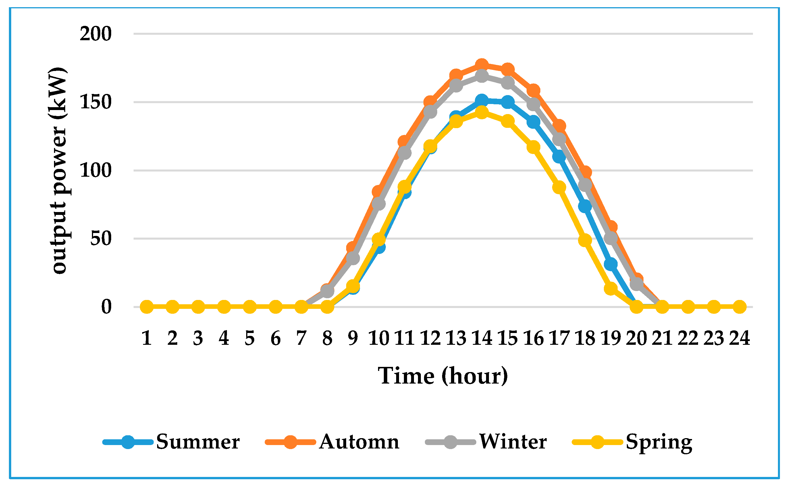
Figure 9.
(a) Summer; (b) autumn; (c) winter and (d) spring average power losses before and after installation DGs and capacitor banks.
Figure 9.
(a) Summer; (b) autumn; (c) winter and (d) spring average power losses before and after installation DGs and capacitor banks.


Figure 10.
(a) Summer; (b) autumn; (c) winter and (d) spring average minimum VSI values before and after DGs installation of DGs and capacitor banks.
Figure 10.
(a) Summer; (b) autumn; (c) winter and (d) spring average minimum VSI values before and after DGs installation of DGs and capacitor banks.

Figure 11.
(a) Summer; (b) autumn; (c) winter and (d) spring average minimum voltage profile values before and after installation of distributed generation and capacitor banks.
Figure 11.
(a) Summer; (b) autumn; (c) winter and (d) spring average minimum voltage profile values before and after installation of distributed generation and capacitor banks.

Table 1.
Input parameters of MOPSO.
| Parameters | Values | Parameters | Values |
|---|---|---|---|
| Maximum number of iteration | personal and global learning coefficient | ||
| Population size | number of grids per dimension | ||
| Repository size | inflation rate | ||
| Weight of inertia | leader selection parameter | ||
| Inertia weight damping rate | deletion selection parameter | ||
| - | - | mutation rate |
Table 2.
Mean and standard deviation of wind speed in (m/s).
| Hour | Summer | Autumn | Winter | Spring | ||||
|---|---|---|---|---|---|---|---|---|
| 1 | 6.6494 | 2.8430 | 4.7376 | 2.7430 | 2.8943 | 2.0355 | 4.2715 | 2.1994 |
| 2 | 6.5817 | 2.9234 | 4.7868 | 2.8272 | 2.9848 | 2.0953 | 4.2765 | 2.2359 |
| 3 | 6.4608 | 2.9960 | 4.8015 | 2.792 | 3.0830 | 2.1464 | 4.1570 | 2.3074 |
| 4 | 6.4045 | 2.9751 | 4.8294 | 2.7389 | 3.0555 | 2.1652 | 4.1213 | 2.2507 |
| 5 | 6.2999 | 3.0546 | 4.7676 | 2.8104 | 3.0863 | 2.2146 | 3.9612 | 2.2083 |
| 6 | 6.1567 | 3.0478 | 4.5511 | 2.8806 | 3.1663 | 2.2676 | 3.7516 | 2.2167 |
| 7 | 6.1769 | 3.1336 | 4.3885 | 2.9969 | 3.2307 | 2.2567 | 3.6082 | 2.2203 |
| 8 | 6.8149 | 3.3058 | 4.6001 | 3.2321 | 3.2307 | 2.2182 | 3.5236 | 2.4315 |
| 9 | 7.4118 | 3.5091 | 5.1490 | 3.4546 | 3.0519 | 2.3307 | 3.7081 | 2.8367 |
| 10 | 7.6581 | 3.5539 | 5.5899 | 3.5169 | 3.6931 | 2.7372 | 4.3216 | 2.9233 |
| 11 | 7.8596 | 3.5666 | 5.7571 | 3.6000 | 4.2409 | 2.7461 | 4.5328 | 2.9701 |
| 12 | 8.0860 | 3.5150 | 5.9031 | 3.7060 | 4.0925 | 2.7464 | 4.6886 | 3.0950 |
| 13 | 8.3195 | 3.4464 | 6.0495 | 3.6553 | 3.8416 | 2.7657 | 4.8413 | 3.1425 |
| 14 | 8.5527 | 3.3354 | 6.1878 | 3.6306 | 3.6964 | 2.6569 | 5.2796 | 3.2220 |
| 15 | 8.6803 | 3.2736 | 6.3495 | 3.4966 | 3.6850 | 2.5886 | 5.7432 | 3.0960 |
| 16 | 8.7671 | 3.1906 | 6.4399 | 3.3369 | 3.7655 | 2.5316 | 6.1633 | 2.9575 |
| 17 | 8.7959 | 2.9993 | 6.5287 | 3.1160 | 3.8253 | 2.4404 | 6.4551 | 2.7951 |
| 18 | 8.5820 | 2.9234 | 6.3463 | 2.9198 | 3.6193 | 2.2015 | 6.4498 | 2.4972 |
| 19 | 8.1864 | 2.8052 | 5.9137 | 2.7845 | 3.2939 | 1.7770 | 6.0105 | 2.2643 |
| 20 | 7.6770 | 2.7069 | 5.4159 | 2.6381 | 3.1292 | 1.6812 | 5.3979 | 2.1585 |
| 21 | 7.2063 | 2.6900 | 5.0096 | 2.6650 | 2.9819 | 1.7519 | 4.60 | 2.0991 |
| 22 | 6.9193 | 2.7132 | 4.7780 | 2.6857 | 2.9160 | 1.8184 | 4.5848 | 2.0543 |
| 23 | 6.7584 | 2.7077 | 4.7549 | 2.7152 | 2.8092 | 1.9225 | 4.4916 | 2.0990 |
| 24 | 6.6819 | 2.7594 | 4.6719 | 2.7343 | 2.8851 | 2.0060 | 4.3096 | 2.2017 |
Table 3.
Mean and standard deviation for solar irradiance in (kW/m2).
| Hour | Summer | Autumn | Winter | Spring | ||||
|---|---|---|---|---|---|---|---|---|
| 1 | 0 | 0 | 0 | 0 | 0 | 0 | 0 | 0 |
| 2 | 0 | 0 | 0 | 0 | 0 | 0 | 0 | 0 |
| 3 | 0 | 0 | 0 | 0 | 0 | 0 | 0 | 0 |
| 4 | 0 | 0 | 0 | 0 | 0 | 0 | 0 | 0 |
| 5 | 0 | 0 | 0 | 0 | 0 | 0 | 0 | 0 |
| 6 | 0 | 0 | 0 | 0 | 0 | 0 | 0 | 0 |
| 7 | 0 | 0 | 0 | 0 | 0 | 0 | 0 | 0 |
| 8 | 0 | 0 | 0.0265 | 0.0165 | 0.0100 | 0.0106 | 0 | 0 |
| 9 | 0.0214 | 0.0321 | 0.1710 | 0.0396 | 0.1360 | 0.0261 | 0.0337 | 0.0352 |
| 10 | 0.1645 | 0.0772 | 0.3705 | 0.0579 | 0.3252 | 0.0491 | 0.1911 | 0.0700 |
| 11 | 0.3491 | 0.1110 | 0.5619 | 0.0739 | 0.5141 | 0.0710 | 0.3714 | 0.0855 |
| 12 | 0.5104 | 0.1413 | 0.7210 | 0.0929 | 0.6718 | 0.0905 | 0.5208 | 0.0962 |
| 13 | 0.6267 | 0.1660 | 0.8359 | 0.0911 | 0.7776 | 0.1079 | 0.6182 | 0.1039 |
| 14 | 0.6902 | 0.1700 | 0.8827 | 0.0976 | 0.8196 | 0.1168 | 0.6545 | 0.1030 |
| 15 | 0.6850 | 0.1636 | 0.8643 | 0.0929 | 0.7929 | 0.1278 | 0.6215 | 0.0998 |
| 16 | 0.6116 | 0.1538 | 0.7745 | 0.0944 | 0.7067 | 0.1319 | 0.5255 | 0.0894 |
| 17 | 0.4819 | 0.1301 | 0.6327 | 0.0834 | 0.5692 | 0.1218 | 0.3784 | 0.0734 |
| 18 | 0.3062 | 0.1035 | 0.4509 | 0.0665 | 0.3979 | 0.0923 | 0.1940 | 0.0580 |
| 19 | 0.1119 | 0.0694 | 0.2494 | 0.0463 | 0.2079 | 0.0668 | 0.0226 | 0.0299 |
| 20 | 0.0038 | 0.0073 | 0.0675 | 0.0278 | 0.04921 | 0.0366 | 0 | 0 |
| 21 | 0 | 0 | 0.0001 | 0.0004 | 0.0001 | 0.0003 | 0 | 0 |
| 22 | 0 | 0 | 0 | 0 | 0 | 0 | 0 | 0 |
| 23 | 0 | 0 | 0 | 0 | 0 | 0 | 0 | 0 |
| 24 | 0 | 0 | 0 | 0 | 0 | 0 | 0 | 0 |
Table 4.
Wind turbine characteristics.
| Parameters | Size |
|---|---|
| Cut-in speed | 3 m per second |
| Rated speed | 12 m per second |
| Cut-out speed | 25 m per second |
| Rated output power | 250 kW |
Table 5.
Solar PV characteristics.
| Parameters | Size |
|---|---|
| Nominal operating temperature | 44 °C |
| Maximum power point current | 8.28 amperes |
| Maximum power point voltage | 30.2 volts |
| Short circuit current | 8.7 amperes |
| Open circuit voltage | 37.6 volts |
| Current temperature coefficient | 0.0045 (amps/°C) |
| Voltage temperature coefficient | 0.1241 (volts/°C) |
Table 6.
Optimization results at the base case and after installation of renewable DGs and capacitor banks in the distribution system.
Table 6.
Optimization results at the base case and after installation of renewable DGs and capacitor banks in the distribution system.
| Ploss (MW) | VSI | VD | |||
|---|---|---|---|---|---|
| Before | After | Before | After | Before | After |
| 7.7641 | 2.3535 | 2629.57 | 2922.35 | 102.41 | 23.51 |
Table 7.
The optimal placement and sizing of renewable DG units and capacitor banks in the distribution system.
Table 7.
The optimal placement and sizing of renewable DG units and capacitor banks in the distribution system.
| Renewable DG Units and Capacitor Banks | Placement | No. of Units | Total Sizing at Location |
|---|---|---|---|
| Wind turbines | 33 | 4 | 1000 (kW) |
| Solar PV | 33 | 4 | 1000 (kW) |
| Biomass | 10 | 1 | 0.812 (MW) |
| Capacitor bank(s) | 30 | 8 | 1000 (KVar) |
Table 8.
The spacing results of MOPSO with proposed test problem and other test problem solved in [48].
Table 8.
The spacing results of MOPSO with proposed test problem and other test problem solved in [48].
| Statistic | Proposed Test Problem | Test Function 1 [48] | Test Function 2 [48] |
|---|---|---|---|
| Best | 0.0427 | 0.043982 | 0.06187 |
| Worst | 0.0859 | 0.538102 | 0.118445 |
| Average | 0.0705 | 0.109452 | 0.09747 |
| Median | 0.0738 | 0.067480 | 0.10396 |
| Std. Dev | 0.0116 | 0.110051 | 0.01675 |
Table 9.
The generational distance results of MOPSO with proposed test problem and other test problem solved in [48].
Table 9.
The generational distance results of MOPSO with proposed test problem and other test problem solved in [48].
| Statistic | Proposed Test Problem | Test Function 1 [48] | Test Function 2 [48] |
|---|---|---|---|
| Best | 0.0085 | 0.002425 | 0.00745 |
| Worst | 0.0204 | 0.476815 | 0.00960 |
| Average | 0.0162 | 0.036535 | 0.00845 |
| Median | 0.0175 | 0.007853 | 0.00845 |
| Std. Dev | 0.0035 | 0.104589 | 0.0005 |
© 2017 by the authors. Licensee MDPI, Basel, Switzerland. This article is an open access article distributed under the terms and conditions of the Creative Commons Attribution (CC BY) license (http://creativecommons.org/licenses/by/4.0/).
Share and Cite
MDPI and ACS Style
Kumar, M.; Nallagownden, P.; Elamvazuthi, I. Optimal Placement and Sizing of Renewable Distributed Generations and Capacitor Banks into Radial Distribution Systems. Energies 2017, 10, 811. https://doi.org/10.3390/en10060811
AMA Style
Kumar M, Nallagownden P, Elamvazuthi I. Optimal Placement and Sizing of Renewable Distributed Generations and Capacitor Banks into Radial Distribution Systems. Energies. 2017; 10(6):811. https://doi.org/10.3390/en10060811
Chicago/Turabian StyleKumar, Mahesh, Perumal Nallagownden, and Irraivan Elamvazuthi. 2017. "Optimal Placement and Sizing of Renewable Distributed Generations and Capacitor Banks into Radial Distribution Systems" Energies 10, no. 6: 811. https://doi.org/10.3390/en10060811
Note that from the first issue of 2016, this journal uses article numbers instead of page numbers. See further details here.