
Large-Eddy Simulations of Two In-Line Turbines in a Wind Tunnel with Different Inflow Conditions


1
Department of Mechanical Engineering, The University of Texas at Dallas, Richardson, TX 75080, USA
2
Dipartimento di Ingegneria Civile e Industriale, Univeristà di Pisa, Pisa 56122, Italy
*
Author to whom correspondence should be addressed.
Energies 2017, 10(6), 821; https://doi.org/10.3390/en10060821
Submission received: 15 May 2017
/
Revised: 10 June 2017
/
Accepted: 14 June 2017
/
Published: 17 June 2017
Abstract
:Numerical simulations reproducing a wind tunnel experiment on two in-line wind turbines have been performed. The flow features and the array performances have been evaluated in different inflow conditions. Following the experimental setup, different inlet conditions are obtained by simulating two grids upstream of the array. The increased turbulence intensity due to the grids improves the wake recovery and the efficiency of the second turbine. However, the inlet grid induces off-design operation on the first turbine, decreasing the efficiency and increasing fatigue loads. Typical grid flow patterns are observed past the rotor of the first turbine, up to the near wake. Further downstream, the signature of the grid on the flow is quite limited. An assessment of numerical modeling aspects (subgrid scale tensor and rotor parameterization) has been performed by comparison with the experimental measurements.
1. Introduction
Currently, turbines operate in clustered configurations or in wind farms. Complex topography or wakes from upstream rotors in wind farms induce spatial and temporal heterogeneity in the incoming flow to a wind turbine. In real applications, wind turbines operate under variable wind direction and intensity and turbulent inflow conditions. Depending on their position in the array, downstream turbines may be impinged by a different turbulent flow than that of the upstream turbines and are then subject to different performances and loads. In fact, the blade aerodynamic performances are quite different from those in ideal design conditions, for which the incoming flow is generally assumed as uniform. A better understanding of the interaction between the incoming wind features and the rotor blades can increase efficiency and reliability. For example, it could lead to improved blade airfoil design or to the development of more effective “smart-rotor” control devices (such as blade flaps or micro-tabs) [1,2,3]. In addition, understanding how turbulence evolves through an array of turbines may allow the development of advanced wind farm control strategies.
The effects of wake interactions and incoming turbulence are normally parameterized in engineering “wake models”, such as in [4,5,6,7]. This is usually achieved by introducing assumptions on the flow behavior (for example, axisymmetry or self-similarity). Such hypotheses involve uncertainties, which need to be quantified to check the accuracy of the results. Moreover, the accuracy of the model may depend on the tuning of empirical parameters.
On the other hand—albeit at higher computational cost—high-fidelity codes based on large-eddy simulations (LES) coupled with rotor models do not require parametrization of the wake and can shed light on the effect of the incoming turbulence on the performances of the array. In fact, LES with actuator line model (ALM) or actuator disk model (ADM) [8,9,10,11] provide a good approximation of the Reynolds stresses in the array. The computational cost of these simulations is still too high for real-time applications for owners and operators. Research efforts are being directed to make LES computationally more affordable by using advanced numerical techniques, as in the recent example of [12]. LES provide rich detailed data, which can be of great value, for example, for tuning the parameters of engineering models, or can provide physical insights to guide wind turbine or wind farm design.
In recent years, several “blind tests” have been organized to assess numerical tools (including LES) with an experimental benchmark [13,14,15,16,17,18,19]. Several experimental and numerical studies are documented in the literature concerning the effects of inflow turbulence on a single wind turbine [20,21,22,23,24,25,26].
The most recent experiment of the blind test series organized at the Norwegian University of Science and Technology (NTNU)—the so-called “Blind Test 4” [18,19]—is considered herein. Two model wind turbines were placed in a wind tunnel, aligned along the mean wind direction. The incoming wind conditions to the array were varied by using two different grids at the entrance of the wind tunnel. A similar study was recently documented in [27], where an active grid system was adopted. Grid turbulence has been widely studied [28,29,30,31], and is a well-suited case to investigate how the turbine rotors modify the incoming coherent structures. This configuration allows the evaluation of the impact of the grid—both on an individual wind turbine with respect to an ideal design condition with uniform flow and no turbulence, and on wake interactions as occur in clustered configurations. The performances of the array were tested in three nominal conditions: low-turbulence uniform inflow, highly turbulent uniform inflow, and highly turbulent shear inflow [19].
In the present work, we present large-eddy simulations results reproducing the three experimental configurations of [18,19]. The aim of this contribution is to study the evolution of the flow field and the performances of the wind turbines for different inflow conditions and to further corroborate the experimental measurements. The exact grid geometry of [19] is reproduced in LES using the immersed boundary technique [32]. In the same way, the geometry of the turbine tower and nacelle is taken into account in our simulations. A similar approach (i.e., using immersed boundary to reproduce typical wind tunnel configurations) has also recently been employed by [33] to obtain turbulent inflow conditions for LES. LES provide a detailed description of the features of the flow impacting on the turbine and their wakes. This permits to appraise the effect of the inflow turbulence in terms of mean flow, turbulent kinetic energy, and coherent structures, and to understand the impact on the turbine performances. Additionally, the comparison with experiments permits the validation of different LES setups, appraising in this way the impact of rotor model and LES turbulence model.
The remainder of the paper is organized as follows. The numerical code is described in Section 2. Details on the LES parameters and on the rotor models are given therein. Section 3 gives some details of the experimental configuration, and explains how it is reproduced in the numerical simulations. Section 4 presents the comparison with the experiments, and analyzes the impact of the turbulent inlet on the flow field and the turbine performances. Finally, Section 5 summarizes the conclusions.
2. Methodology
2.1. Governing Equations and Turbulence Modeling
The non-dimensional filtered incompressible Navier–Stokes equations are considered. The filtering operation is implicit; i.e., it is assumed that the numerical discretization acts as a filter. By using the Einstein notation, the governing equations are the following:
where are the filtered velocity components. The Reynolds number is , with the undisturbed upstream velocity, the diameter of the second turbine, and the kinematic viscosity of the air. The modified pressure is the sum of the filtered pressure and of the isotropic part of the subgrid-scale (SGS) tensor . The deviatoric part is modeled as described in detail later on. The term represents the component of the body forces introduced to model the effects of the turbine blades on the aerodynamic field, as explained in Section 2.2.
To model the SGS terms, we considered eddy-viscosity models, which are based on the following Boussinesq’s hypothesis:
where is the filtered strain rate tensor and is the subgrid (or eddy) viscosity. The expression of the eddy-viscosity differs according to the particular model considered.
The first SGS model used in the present work is the classical Smagorinsky model [34], in which the subgrid viscosity is expressed as follows:
where is the model constant and is the filter width. Since—as previously said—filtering is implicitly applied by numerical discretization, we use the following definition: , with being the grid cell width in the i direction. It is well known that this model has an incorrect behavior near solid walls, and ad-hoc damping of the eddy viscosity is usually employed to overcome this problem. However, in our case, due to the complex geometry of tower and nacelle and to the immersed boundary treatment (see Section 2.3), this would be extremely complex; therefore, no damping is used. In spite of its limitations, we consider the Smagorinsky model, because it is the most widely employed SGS model in LES of wind turbine flows.
The more recent -model [35] is also considered. The SGS viscosity is expressed as a function of the singular values of the filtered velocity gradient tensor, , as follows:
where is the model constant. This model has the appropriate behavior in the vicinity of solid boundaries without requiring any ad-hoc treatment.
Both of the SGS models are local and static. However, numerical results show that the -model is moderately more computationally expensive—most likely because of the computation of the singular values. The cpu-time per time step is about larger than for the Smagorinsky model, which is similar to the results reported in [35]. Therein, an alternative and more efficient method to compute the singular values is also proposed, but was not tested in the present paper.
2.2. Rotor Modeling
The rotating blades of the wind turbines have been modeled as body forces introduced in Equation (2). Two different approaches have been pursued; namely, the actuator line model (ALM) and the rotating disk actuator model (RADM).
The ALM [36] distributes the blade forces along rotating lines. At each generic section of the rotating blades (Figure 1a), the flow velocity relative to the airfoil, , and the angle of attack, , are computed as follows:
with the local twist angle of the blade, the angular velocity of the blades, r the distance of the considered airfoil from the center of the rotor, the streamwise velocity, and the azimuthal velocity on the rotor plane (see Figure 1a).
By dividing each blade in a discrete number of sections, it is possible to express the lift and the drag per unit length of the airfoil as follows:
where c is the airfoil chord, are the lift and drag coefficients, which are assumed to be known functions of . The actuator line model consists of projecting the aerodynamic force , which is the vector sum of L and D, onto the flow field, by using a Gaussian function which is spread on a cylinder with axis coincident with each actuator line. Therefore, by defining the Gaussian regularization kernel:
the force —which is the result of the spreading—can be expressed as follows:
where s is the distance from the actuator line. The parameter determines the area (cross-section) of the cylinder, , and hence how the force spreading is performed. As reported in [37], the parameter should be such that , where is the grid cell size in the direction of the rotor axis. This condition should be respected for an oscillation-free numerical solution. In the present simulations, has been used.
The rotating actuator disk model (RADM) [38] is another approach based on force spreading. It is similar to the ALM in many aspects, with the main differences related to the spreading distribution. The forces are computed in the same way as in the ALM, but in RADM they are spread on a disk, in the axial and in the azimuthal directions, as follows:
In Equation (12), is the relative distance in the streamwise direction of the considered point from the rotor position (), while is the relative angular distance from the angular position of the blade . B is the number of blades; in the present case, . For three-bladed wind turbines, the force on each blade is distributed in a sector of . The parameter for the RADM expresses the thickness of the disk. It is analogous to the spreading width of the ALM in Equation (10), although in this case it regulates the force distribution in the streamwise direction x only. Similarly as for the ALM, it has been selected as .
An example of the thrust force distribution on a rotor for the ALM and RADM is shown in Figure 1b. In both ALM and RADM, the rotation of the blades is preserved, but the RADM is expected to provide a lower accuracy than the ALM in the representation of the smallest flow scales (for instance, the tip vortices). On the other hand, because the force spreading in the RADM is smoother than the one of ALM, larger time steps can be used in the simulations with the RADM. This leads to much lower computational costs than with the ALM, given that the cpu-time per time-step is essentially the same for the two models. A simulation with RADM is about six times faster than using ALM.
2.3. Numerical Scheme
The discretisation method for Equations (1) and (2) is discussed in [39]. It is based on a central finite-difference method with second order accuracy in time and in space. The computational grid is Cartesian and staggered in order to avoid spurious pressure modes and the presence of checkerboard patterns. Integration in time is performed with a fractional step method which employs the Crank–Nicolson scheme [39] for the linear terms (treated implicitly), and a low-storage third-order Runge–Kutta method [40] for the non-linear terms, which are treated explicitly. In order to reduce the computational costs, an approximate factorization technique [41] is used to invert the resulting linear system matrices at each time step. The momentum equations are solved by using the pressure at the previous time step, obtaining in this way a non-solenoidal velocity field. In order to satisfy the mass balance, the solution is then projected onto a solenoidal space obtaining the next step velocity field.
For the modeling of tower, nacelle, and other kinds of bodies, the immersed boundary method (IBM) [32] has been adopted. It consists of setting the velocity equal to zero in those grid-points which are inside the volume occupied by the body. A correction to the first and second derivative is applied to the external points closest to the body boundaries by using the effective distance from the body rather than the computational mesh spacing for the computation of the derivatives. The presence of complex geometries can be includeded in computationally efficient Cartesian grids with this method.
3. Simulation Setup
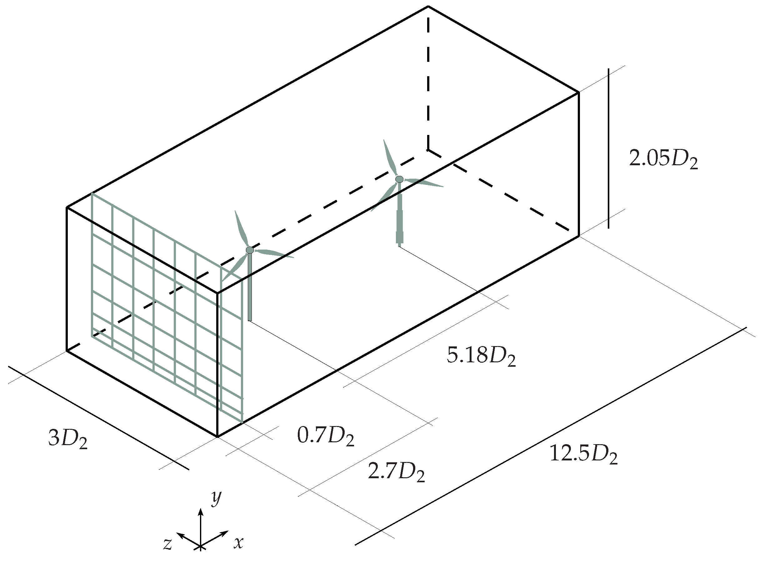
The numerical simulations reproduce the experiments carried out in the closed-loop wind tunnel of the Norwegian University of Science and Technology (NTNU) in the framework of the “Blind test 4” workshop [18]. Two wind turbine models were placed inside the wind tunnel at NTNU, aligned along the wind direction. Figure 2 shows a sketch of the experimental and numerical setup.
Both wind turbines have the same blades, but different tower and nacelle. The geometry of the turbine models is available in the blind-test invitation document [18]. Figure 3 shows the overall layout of the models. The towers were fixed to a support beneath the tunnel floor to have the same hub height . Because of the different nacelle geometry, the two turbines have different rotor diameters, equal to and for the first (upstream) and second (downstream) turbine, respectively.
In the experiment, free-stream conditions were varied by placing grids at the entrance of the test section. A uniform grid with square rods of size and spacing was used to obtain a uniform mean flow with turbulence intensity () of about at the location of the first turbine. A second grid was also used, with a modified vertical arrangement of the bars with respect to the uniform grid. The horizontal bars were clustered closer to the tunnel floor [18] to obtain a mean shear inflow and approximately the same turbulence intensity. In the numerical simulations, the grids are reproduced using the IBM [32].
The mesh employed for the LES of the wind turbine experiment consists of grid-points uniformly spaced in the x, y, and z directions, respectively. With this resolution, about 120 grid-points are present along a rotor diameter. This is quite a bit larger than typical values employed in LES with actuator line or, particularly, disk. However, a finer grid resolution permits the evolution of the flow to be described more accurately, particularly past the immersed boundaries. No-slip condition is imposed on the boundary of the domain in order to reproduce the wind tunnel walls, as well as on the turbine tower and nacelle. Van Driest damping [42] is used at the first grid point away from the wall for the streamwise and spanwise velocity (and the second for the wall normal velocity, since the first is on the wall). At the inlet of the computational box, a uniform velocity is prescribed. When present, the grid is placed at ; that is, two diameters upstream of the first rotor as specified in [18]. Sommerfeld radiation conditions are used at the outlet of the domain [43].
Three test cases are defined based on the use of the grids at the entrance of the wind tunnel: (i) no grid, (ii) uniform grid, and (iii) non-uniform grid case. For each configuration, four different combinations of rotor parameterizations and subgrid models have been tested, as summarized in Table 1.
Following [18], the turbines are operated at constant tip-speed ratio. The tip-speed ratio is defined for both turbines using the free-stream reference velocity, and is set equal to:
where is the angular velocity of the ith turbine and is the rotor radius. Note that corresponds to the tip-speed ratio of maximum efficiency for the first turbine, so that in the no-grid case the turbine is operating in design conditions.
4. Results
Numerical results are analyzed and compared with the experimental measurements in the following sections. Statistics have been computed using averages over time, as defined by the following:
where denotes a generic variable, the overline is used to denote the time-average, and represents initial transient. The value of the sampling time T has been chosen in order to ensure the convergence of the statistics, and it corresponds to at least 70 rotor revolutions for the slowest rotating turbine. A prime is used to indicate the fluctuations: .
Unless stated otherwise, all variables presented in the following are conveniently normalized using the reference velocity and the diameter of the second turbine .
4.1. Simulations of the Empty Wind Tunnel
A set of LES of the empty tunnel with only the grids at the inlet was run. For these simulations, the Smagorinsky model (with ) and a coarser grid () were used. The objective of this preliminary study was to appraise the base flow due to the inlet grids.
Figure 4a shows the streamwise decay of the RMS velocity fluctuations for the uniform grid case. The numerical results are in good agreement with the experimental measurements [18] and with the theoretical behaviour [44,45]:
In Equation (17), is the streamwise distance from the location of the grid , and d is the square rod dimension. As reported in [45], for square-bar grids. Figure 4a shows that the turbulence generated by the grid is not perfectly isotropic, since is larger than the other two components.
This is further corroborated by the vertical profiles of the anisotropy function F [46,47]:
where and are, respectively, the second and third invariant of the anisotropy Reynolds stress tensor . In isotropic turbulence, F is unity [46,47,48]. As shown in Figure 4b, close to the grid (; that is, one diameter upstream of the first turbine) the flow is strongly anisotropic, with a clear influence of the geometric details of the grid. Proceeding downstream, turbulence is gradually redistributed and along the rotor area in front of the second turbine position (). On the other hand, due to dissipation, turbulence intensity significantly decreases moving downstream.
4.2. Simulations of the Two-Turbine Array
Unless stated otherwise, the results shown in the following sections are those obtained with ALM and Smagorinsky model (). The results of the other LES setups (Table 1) are quite similar from a qualitative point of view. Nonetheless, the specific differences among the various setups are also detailed in the following, using the experimental data.
4.2.1. Mean Flow
Figure 5 shows the mean flow field in the vertical plane through the tower axes for the three different cases. The first turbine extracts energy from the incoming flow and generates a large velocity deficit. The wake propagating downstream impinges on the second turbine, which further extracts momentum from the flow. The flow strongly accelerates between the rotor and the upper wall of the tunnel because of the blockage.
A recirculating region can be observed behind the tower of both turbines. On the first turbine, the length of the recirculation bubble shortens proceeding from the tunnel floor upward in to the rotor region. The wake shed from the turbine blades interacts with the flow behind the tower cylinder and deflects the tower wake laterally (i.e., outside the vertical plane shown). On the second turbine, the recirculation length seems to conserve the imprint of the “piece-wise” geometry of the tower, although many parameters (notably blade–tower interaction) influence the flow behind the tower and concur to determine the length of the recirculating region.
The presence of the grid significantly affects the incoming flow on the first wind turbine. The distance between the first turbine and the upstream grid is quite small because of the limitations imposed by the tunnel dimensions on the experimental layout. The streaks of high velocity flow generated by the open meshes and the wakes of the grid bars are still evident at the rotor location and beyond.
Figure 6 shows the velocity averaged over the rotor disk area along the streamwise direction:
where is the area swept by the blades of the first turbine. To some approximation, the rotor velocity describes the evolution of the flow through the array. The drag of the inlet grids causes a momentum loss upstream of the array. The drop due to the uniform grid is larger because the “local” solidity of this grid in the rotor area is larger than that of the non-uniform grid.
The velocity deficit across the first rotor is similar in the various cases, despite the differences in the incoming wind. The turbine is set to maintain a constant tip-speed ratio, which is defined as in Equation (14) using as the reference velocity the wind speed upstream of the grid . In the case of the uniform grid (Figure 5b), the first turbine is actually operating at an effective tip-speed ratio , which is larger than the reference one because . While this involves a larger non-dimensional thrust coefficient, the actual thrust force scales with the square of the effective incoming wind speed. The overall effect is that the turbine thrust force is reduced, and the velocity downstream of the turbine is similar to that of the other two cases.
However, the wake evolves quite differently downstream, whether a grid is present or not. The slope of the rotor velocity increases for the inlet-grid cases between . Wake recovery is enhanced and the trailing turbine experiences a higher wind speed.
The wake of the second turbine is less affected by the variation of the wind tunnel entrance conditions. The three curves have a similar slope, but are shifted according to the velocity upstream of the rotor. The mean velocity downstream of the second turbine seems mainly determined by the speed of the incoming wake from the first turbine.
At this scale, the grids do not seem to have a further impact on the flow behind the second turbine. However, it should be noted that the rotor average filters smaller-scale features, the average area being significantly larger than the mesh size of the grid ().
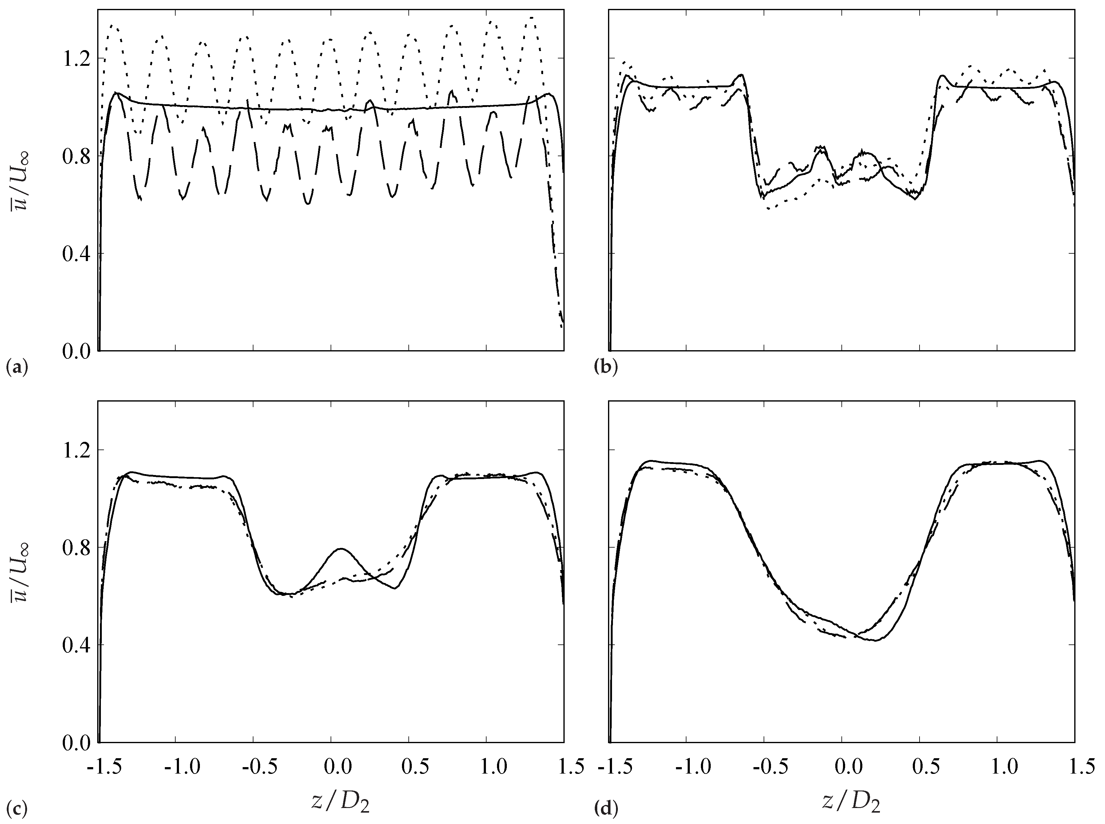
Average velocity profiles evidence some of these features. The spatial heterogeneity induced by the grid in the mean flow can be observed in Figure 7a, which shows a spanwise profile upstream of the first turbine. The difference in the mean velocity at hub height between the cases with the grid is due to the different vertical arrangement of the horizontal bars. In the non-uniform grid case, the velocity profile happens to be in the wake of one of the horizontal bars (Figure 5).
At a distance of downstream of the first turbine (Figure 7b), the streaky pattern generated by the grid is still visible in the near wake, although partly homogenized by the wake structures. Further downstream at a distance of from the first rotor (Figure 7c), the spanwise gradients have been diffused. Across both the external flow and the wake, the profiles of the two grids are hardly distinguishable from each other. However, the impact of the grids on the evolution of the wake is noticeable compared to the case without grid at the inlet. The wake is not fairly symmetric as in the no-grid case, but is skewed towards a side. Due to the merger of the regions of accelerated flow around the nacelle (visible also in Figure 7b), the central jet is not observed when a grid is present at the inlet, but is rapidly diffused by the background mixing.
The similarity between the two grid cases is even more remarkable after the second rotor, while some residual differences persist with the case without grid (Figure 7d). Comparing Figure 7c,d, it seems that an asymptotic “self-similar” profile is achieved earlier upstream for the cases with a grid at the inlet, even before the second turbine.
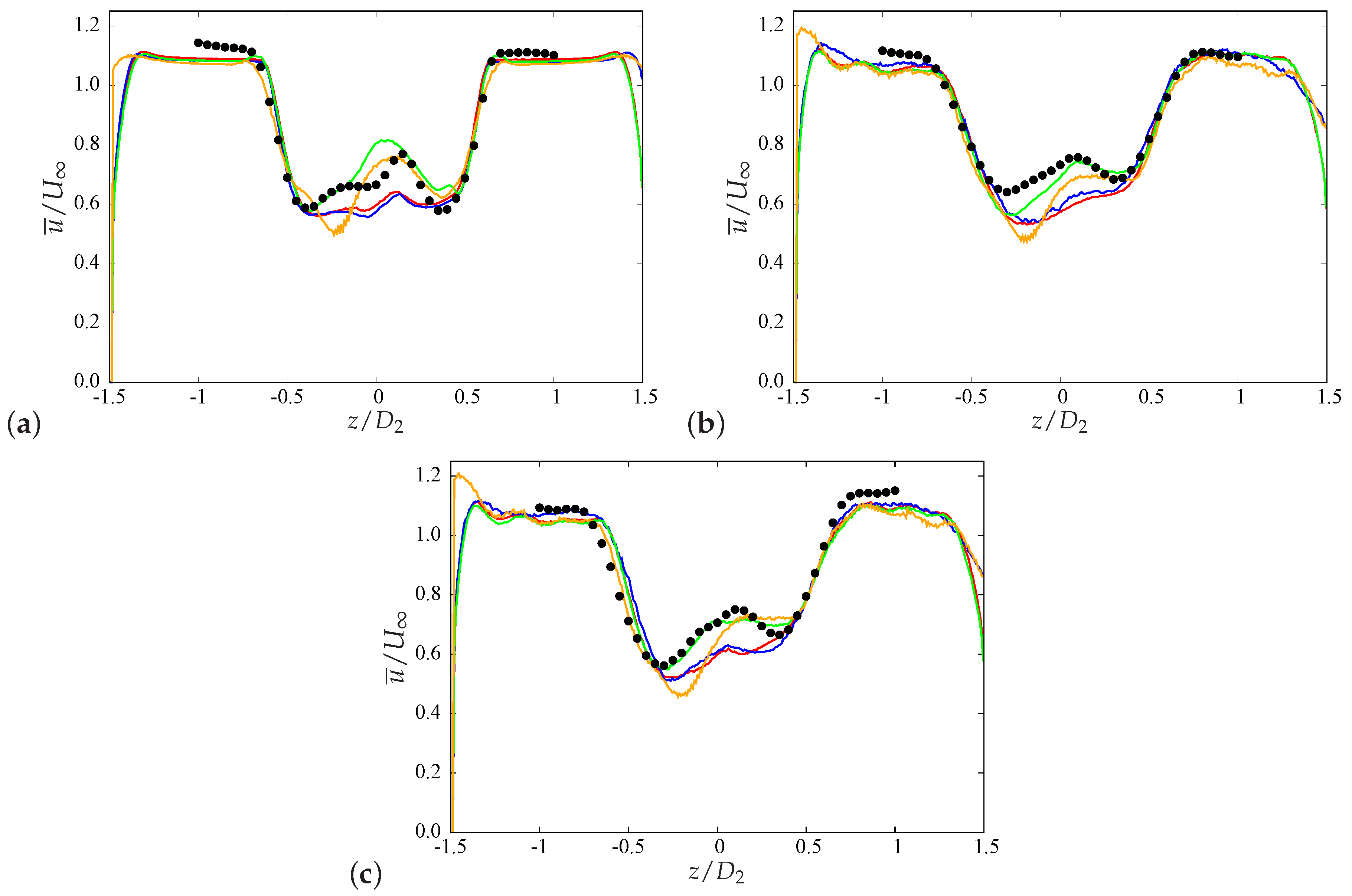
Figure 8 compares the present LES results obtained with different sub-grid scale models with the experimental measurements. It shows a spanwise profile of the mean velocity downstream of the first rotor. Overall, LES results provide a reasonable agreement with the experimental data. While the external shear layers are accurately predicted by the various simulations, some differences are observed in the wake core. Figure 8 suggests that the impact of the turbine model is predominant on that of the SGS modeling, which is consistent with previous studies (e.g., [49]).
The RADM generally provides a more symmetric and uniform field in the wake of the turbine. This is due to the force spreading, which smoothes out small-scale wake characteristics. Consistently, when the RADM is employed, the use of different SGS models results only in minor changes to the velocity profile. On the other hand, when the ALM is adopted, a more detailed and accurate description of the flow can be achieved. The LES with ALM and Smagorinsky model () provides the best results throughout the three experimental setups. The sensitivity to the sub-grid model is also increased with the ALM. Large differences can be observed in the core of the wake when the model constant is changed from to (an almost no-model configuration).
The present results suggest that the effects of the SGS modeling on low-order statistics and global flow features are limited. However, the amount of introduced dissipation seems to have a significant impact—at least combined with ALM. Furthermore, it is interesting that the sensitivity to SGS modeling is practically independent of the inflow conditions. Consistently with the present results, Sarlak et al. [49] found the impact of the SGS on the flow structures and on the predicted power performance to be small compared to that of rotor modeling, although for a different configuration and simulation setup.
4.2.2. Turbulent Kinetic Energy
Figure 9 shows a visualization of the turbulent kinetic energy (TKE) in the horizontal plane at hub height. The TKE is defined as:
The grid at the entrance of the wind tunnel generates a large amount of TKE. As observed for the velocity field (Figure 5), the TKE is not uniform over the tunnel cross-section, but is modulated by the geometry of the inlet grid.
In the wake of the first turbine, high values of TKE are observed at the edges of the wake. These are due to the thin shear layer caused by the velocity deficit, and to the periodic passage of tip vortices shed by the blade. A large turbulent intensity is also found in the core of the near wake, due to the presence of tower and nacelle. The wake of the tower and nacelle is tilted laterally because of the swirl imparted by the rotor to the flow [50]. Proceeding downstream, the wake of the tower is advected towards the edge of the rotor. The interaction with the tip vortices causes the vortex breakdown and increases the value of the TKE.
For the cases with the grid, the levels of TKE in the wake are generally higher. The interaction between the wake from the nacelle and the tip vortex occurs earlier upstream. The lateral distortion of the wake is more evident in the cases with grid also from the mean velocity profiles (Figure 7).
Nonetheless, the inflow to the second turbine is similar among the three cases. The wake from the first turbine is also undergoing a transition to turbulence in the “clean” inlet case, although not uniformly across the rotor span. Minor differences can be observed in the evolution of wake past the second rotor.
Moreover, the turbulence generated by the grid at the inlet is decaying along the streamwise direction. The flow surrounding the wake region has a quite low turbulence intensity downstream of the second turbine, compared to levels outside the wake of the first turbine. This limits the mean kinetic energy entrainment in the wake. As shown in Figure 6, the recovery of the second turbine wake is rather unaffected by the presence of the grid at the tunnel entrance.
In Figure 10, spanwise profiles at hub height of TKE obtained from the different LES simulations are compared with the experimental data acquired at the same location of the velocity measurements (Figure 8); that is, downstream of the first turbine. The shape of the profile is correctly predicted (especially by the ALM simulations), although the TKE is generally underpredicted. This could be expected since only the resolved part of TKE is explicitly obtained in LES and is plotted in Figure 10. Compared to the velocity measurements, the agreement with the experiments is slightly worse.
The sensitivity to the simulation parameters (rotor and sub-grid scale models) generally follows the same trend observed for the mean velocity profiles. However, the impact of the rotor model appears to be a little more moderate, especially for the cases with inlet grids (Figure 10b,c). The large-scale heterogeneity of the incoming turbulence overcomes the effects of the individual blade motion, which are of a smaller scale. Hence, the shortcomings of the RADM are reduced in the cases with the grid.
Analogously, the different sub-grid scale models (-model and Smagorinsky model, coupled with RADM) do not significantly affect the results. As expected, reducing the Smagorinsky constant from to allows more energy to be retained in the resolved field, and the profiles are closer to the measurements. Overall, the TKE is affected by the SGS model to a larger degree than the mean velocity.
4.2.3. Wake Structures
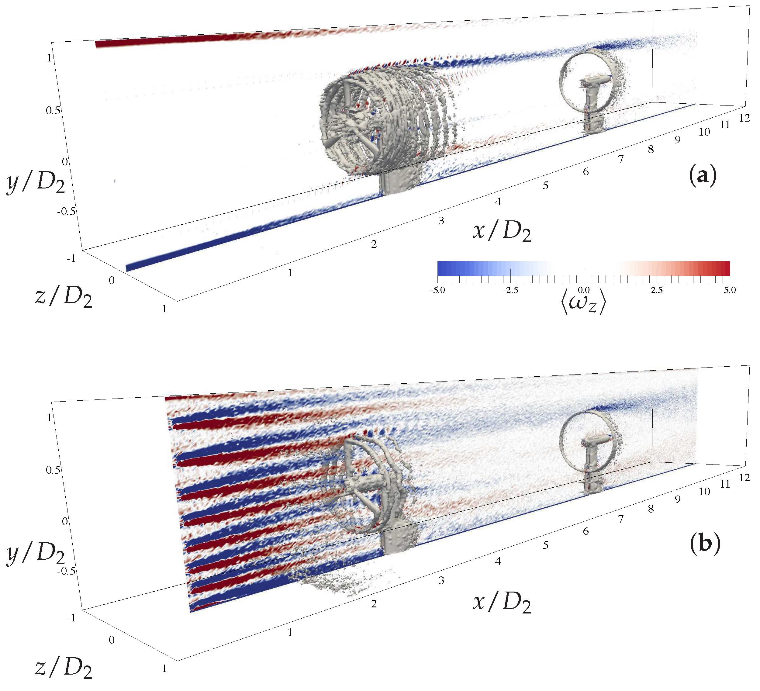
The presence of the grids at the inlet also affects the evolution of the flow in a qualitative manner. Figure 11 shows the impact of the flow patterns generated by the grid on the coherent structures in the wake of the first turbine. The coherent structures in the wake are educed using phase-averaged vorticity [51]. A phase average for the ith vorticity component is here defined as:
where denotes an instant in time for which one of the blades of the first turbine is parallel to the tower axis and points upwards. indicates the total number of fields for which this condition occurs. Note that an analogous phase-average can be defined considering the position of the downstream turbine blades when sampling the time instant for the phase-average, rather than the first turbine rotor. In this way, one would focus on the coherent structures in the wake of the second turbine (see Figure 12).
The iso-surfaces of in Figure 11 at the rotor plane evidence the disposition of the first turbine blades for the phase selected. The trace of the blade positions of the second turbine is not observed. At the time instants , they can occupy any azimuthal position, and the presence of the bound vorticity over the blade is not retained on average.
The visualisations show that the breakdown of the tip vortex helicoidal path occurs earlier (i.e., more upstream) in the presence of the non-uniform grid at the inlet. The entrainment of mean kinetic energy into the wake is enhanced after the tip vortex breakdown [50]. Thus, the wake recovery is faster for the non-uniform grid case than the “clean” inlet case (Figure 6).
The contours of phase-averaged spanwise vorticity in the vertical plane show that the alternating grid pattern persists past the rotor of the first turbine for some distance downstream before being eventually smoothed by turbulent diffusion and by the interaction with the turbine wake. This feature has also been observed for the mean velocity profile in the near wake of the first turbine (Figure 7b).
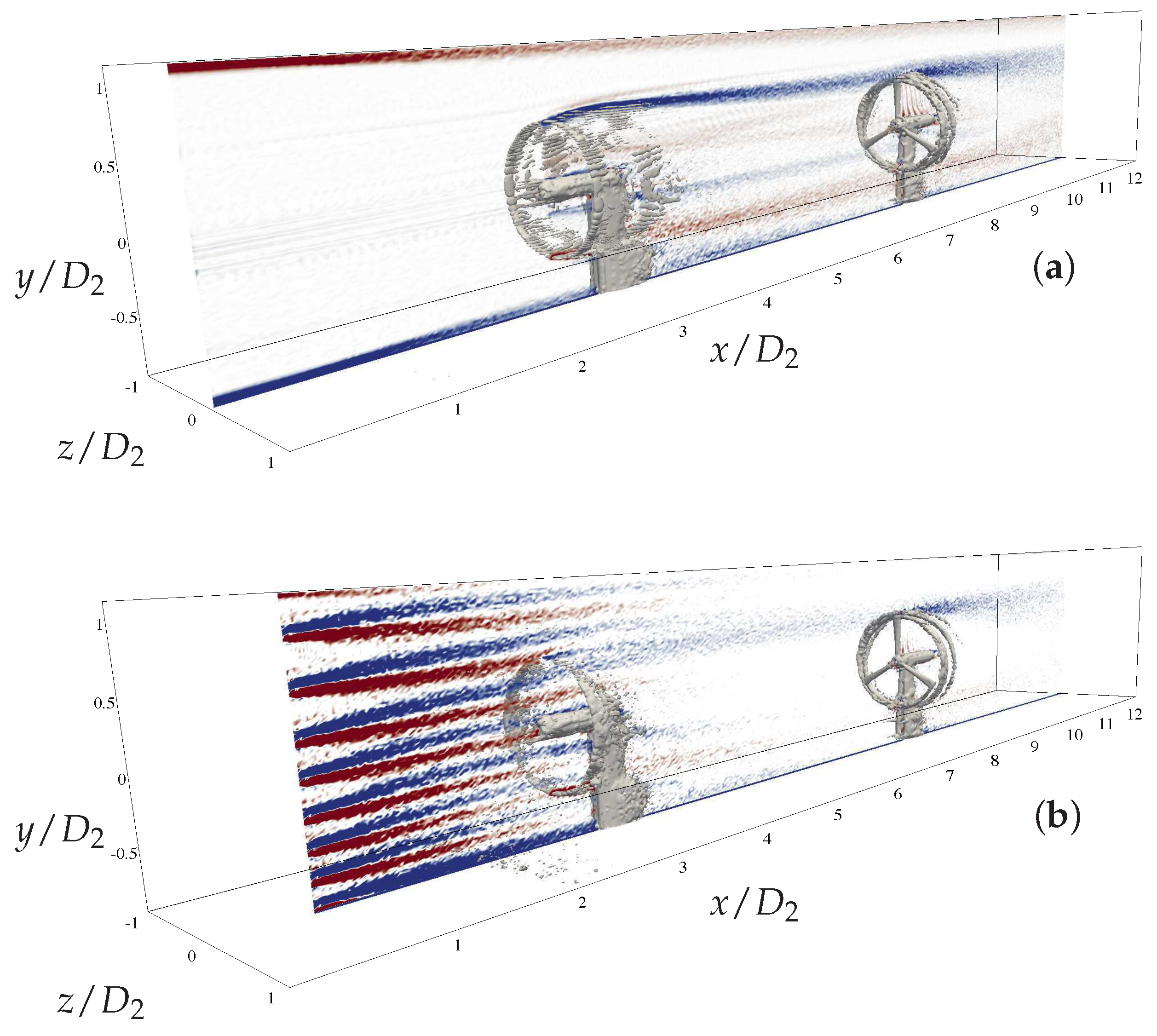
Figure 12 shows visualisations of the phase-averaged vorticity for the second turbine. That is, the average is performed as defined in (21), but the condition on the time instant is now that a blade of the second turbine is in the vertical position. Compared to Figure 11, the imprint of the blades is visible on the second rotor, while it is filtered on the first turbine.
The coherent structures of the second turbine are not much affected by the grid. The incoming flow is similar in both cases and is turbulent. The helicoidal pattern breaks down quite rapidly after a few revolutions, similarly in both cases (Figure 12).
4.2.4. Performances
The performances of the wind turbines are described in terms of power and thrust coefficients:
where is the power produced by the ith turbine, and is the thrust force—that is, the integral of the aerodynamic forces on the rotor in the axial direction. is the rotor area of the ith turbine. Figure 13 shows the comparison of the numerical results with the values of and measured experimentally. The agreement is rather good for the power production, while the thrust coefficient is generally under-predicted. The sensitivity to the rotor model is quite limited—especially on the first turbine. Larger differences are found on the second turbine. The actuator line model is generally closer to the experiments, probably because of a more accurate description of the wake evolution.
As for the SGS modeling, the predictions of the -model and the Smagorinsky model coupled with RADM do not change significantly. Larger discrepancies are observed on the ALM for the two different values of the Smagorinsky constant. This changes the level of SGS dissipation, which influences the wake evolution as observed for the mean velocity and TKE (Figure 8 and Figure 10).
The presence of the grid affects the turbine performances. The power production of the first turbine is reduced compared to the no-grid reference case. This can be related to the incoming turbulence intensity of the grid cases. The tip-speed ratio assumes instantaneous off-design values because of wind fluctuations.
The close distance from the grid also contributes to the downgraded performances. The time-averaged incoming velocity shows a strong spatial heterogeneity. This affects the distribution of angle of attack, which is shown in Figure 14a. Even if on average the turbine is working at the ideal tip-speed ratio (), the mean angle of attack is different from the design conditions (which are represented by the no-grid case).
Figure 14b shows the time-averaged angle of attack along a blade of the second turbine. Departures from the ideal conditions are also observed in this case. However, due to the faster wake recovery of the grid cases (Figure 6), the efficiency of the second turbine is increased compared to the reference case.
The turbulence intensity generated by the grid promotes the recovery, but inevitably induces fluctuating loads on the turbines. Figure 15 shows the RMS fluctuations of the angle of attack along the blade span. The first turbine is directly exposed to the grid turbulence, and the fluctuations increase significantly. In the absence of the grid, the fluctuations at the root are caused by the disturbances induced by the nacelle and the blade geometry. The sharp transition from the cylinder that connects the blade to the nacelle and the airfoil section induces flow separation, and thus local unsteadiness. In the ALM and RADM, this is accounted for by the different aerodynamic coefficients at the various sections of the blade.
Conversely, the conditions on the second turbine are not much changed in terms of by the inlet grid. The fluctuations in the angle of attack are mostly determined by the unsteadiness of the incoming wake, which dominates over the background turbulence.
The fluctuations in the angle of attack give rise to unsteady loads, which can reduce the structural integrity of the turbine. Although a rigorous and detailed analysis of the fatigue behavior requires a fluid-structure interaction simulation, nonetheless the aerodynamic loads obtained from LES provide qualitative information and relative assessments. A standard measure of the fatigue damage is the damage equivalent load (DEL) [52]. The DEL is the constant amplitude of an equivalent alternating load that produces the same fatigue damage as the actual load time history [52,53]. Figure 16 shows the DEL for the axial force on the first and second turbine in the three cases considered. The fatigue load on the first turbine is increased by almost an order of magnitude when the grids are placed upstream of the wind tunnel. The DEL is almost of the mean axial load, which is comparable to the level of the second turbine. The fatigue loads induced by the presence of the grid are nearly the same as those of a waked turbine. The influence of the grids on the second turbine fatigue loads is marginal, consistently with the previously observed trends. From a practical point of view, this limited dependence on the upstream inflow conditions observed on the second turbine may be positively regarded in an actual wind farm for scheduling maintenance procedures. In fact, it may be inferred from the present results that turbines which mostly operate in waked conditions would have similar fatigue damage regardless of the position in the wind farm.
Figure 17 shows the spectra of the power production of the two turbines. Only the cases without the grid and with the non-uniform grid are shown to avoid crowding.
On the first turbine (Figure 17a), a clear peak at three times the turbine rotational frequency () is observed in both cases. However, when the grid is placed at the inlet of the wind tunnel, the peak is not as sharp as in the no-grid case, but is smoothed out. This may be related to the instantaneous variations of the effective tip-speed ratio due to the wind fluctuations.
At high frequency, the no-grid case follows a Kolmogorov scaling [54]—a feature which has been found to characterize wind turbine power outputs in actual wind farms [55]. This is not the case for the non-uniform grid spectra. Further downstream, on the second turbine (Figure 17b), both signals adjust to the slope.
The spectra of the second turbine are similar for both configurations. The peak related to the turbine rotational frequency () is smoothed over a range of frequencies. A spectral contribution connected with the angular frequency of the first turbine also contributes to the spreading of the peak. The low-frequency peak is probably related to the large-scale meandering of the wake of the first turbine.
5. Conclusions
Numerical simulations reproducing a wind tunnel experiment on two in-line wind turbines have been performed. Following the reference experimental configuration, the inflow conditions have been varied by using grids at the inlet, which were simulated using the immersed boundary method.
The turbulence generated by the grid has a significant effect on the flow and the array performances. The grids degrade the performance of the first turbine, increasing the wind fluctuations over the blade. Because of the close distance from the grid, a strong heterogeneity characterizes the mean field. The not-fully-developed state of turbulence at the first rotor positions also affects the power spectra, which does not show a characteristic Kolmogorov slope.
On the contrary, the second turbine benefits from an increased recovery rate of the first turbine wake, which results in increased efficiency. The ambient turbulence intensity due to the grid promotes entrainment of mean kinetic energy, anticipating the tip vortex breakdown. Because of the decay of grid turbulence with the streamwise direction, the recovery of the second turbine wake is similar to the case with no grid.
The presence of the grid has a rather limited influence on the second turbine, besides the increase in the incoming wind speed. A residual signature can be observed from the mean distribution of the angle of attack, which may be affected by a slight tilting of the first turbine wake in the cases with the grid. On the other hand, the fluctuating angle of attack is not much changed on the blade of the second turbine.
Consequently, the fatigue loads on the second turbine also maintain a quite similar level for the various simulations. On the contrary, the fatigue damage considerably increases on the first turbine when it operates downstream of the grid.
Such limited influence of the grid on the second turbine may be explained by the fact that the characteristic feature of the grid persists only in the near wake of the second turbine. The interaction with the wake of the first turbine and the natural decay of the grid flow contributes to the dissipation of such structures by the time the position of the downstream turbine is reached. The independence of the second turbine from the inlet conditions suggests that a two-turbine may be viewed as “minimal unit” to study wake interactions. For example, LES of wind farms in the literature [9] report that the power production of the wind turbines (when the wind direction is such that a column of wake is formed) seems to reach a plateau after the second row. However, further investigations are necessary to provide stronger support about the validity and generality of this hypothesis.
The comparison with experimental results is satisfactory. The wind turbine performances are predicted quite well. A good agreement with the measurements was observed for the mean velocity profiles. On the other hand, the turbulent kinetic energy in the wake was generally underestimated.
As far as the LES modeling is concerned, the present results confirm general trends observed in the literature. The actuator line model provides the best accuracy, but the shortcomings of the rotating disk are reduced in the cases with the grids. The larger integral length scale of the incoming flow shadows the disadvantages of the larger force spreading. This may be helpful from a practical point of view, because the rotating disk allows for larger simulation time steps, although the entrainment is somewhat underpredicted. As for the subgrid tensor, a limited sensitivity of the global flow features and of the turbine performances to SGS modeling was observed, although the results highlight the importance of the introduced SGS dissipation, at least in combination with ALM. It is interesting that the impact of the SGS modeling remains limited independently of the inflow conditions. A larger impact of SGS modeling could be expected for a more detailed analysis of small-scale flow features and dynamics, which is beyond the scope of the present work. More advanced SGS models would probably also improve the TKE prediction in the wake.
Acknowledgments
Stefano Leonardi was supported by NSF PIRE WINDINSPIRE (grant No. 1243482).
Author Contributions
Authors contributed equally.
Conflicts of Interest
The authors declare no conflict of interest.
References
- Barlas, T.K.; van Kuik, G.A.M. State of the art and prospectives of smart rotor control fow wind turbines. J. Phys. Conf. Ser. 2007, 75, 012080. [Google Scholar] [CrossRef]
- Van Wingerden, J.W.; Hulskamp, A.W.; Barlas, T.; Marrant, B.; van Kuik, G.A.M.; Molenaar, D.-P.; Verhaegen, M. On the proof of concept of a ‘smart’ wind turbine rotor blade for load alleviation. Wind Energy 2008, 11, 265–280. [Google Scholar] [CrossRef]
- Lackner, M.A.; van Kuik, G. A comparison of smart rotor control approaches using trailing edge flaps and individual pitch control. Wind Energy 2010, 13, 117–134. [Google Scholar] [CrossRef]
- Katić, I.; Højstrup, J.; Jensen, N.O. A simple model for cluster efficiency. In Proceedings of the European Wind Energy Association Conference and Exhibition, Rome, Italy, 7–9 October 1986. [Google Scholar]
- Larsen, G.C. A Simple Wake Calculation Procedure; Technical Report Risø-M-2760; Risø National Laboratory: Roskilde, Denmark, 1988. [Google Scholar]
- Ainslie, J.F. Calculating the flowfield in the wake of wind turbines. J. Wind Eng. Ind. Aerodyn. 1988, 27, 213–224. [Google Scholar] [CrossRef]
- Frandsen, S.; Barthelmie, R.; Pryor, S.; Rathmann, O.; Larsen, S.; Højstrup, J. Analytical modelling of wind speed deficit in large offshore wind farms. Wind Energy 2006, 9, 39–53. [Google Scholar] [CrossRef]
- Calaf, M.; Meneveau, C.; Meyers, J. Large eddy simulation study of fully developed wind-turbine array boundary layers. Phys. Fluids 2010, 22, 015110. [Google Scholar] [CrossRef]
- Churchfield, M.; Lee, S.; Moriarty, P.; Martinez, L.; Leonardi, S.; Vijayakumar, G.; Brasseur, J. A large-eddy simulation of wind-plant aerodynamics. In Proceedings of the 50th AIAA Aerospace Sciences Meeting, Nashville, TN, USA, 9–12 January 2012. [Google Scholar]
- Wu, Y.T.; Porté-Agel, F. Atmospheric turbulence effects on wind-turbine wakes: An LES study. Energies 2012, 5, 5340–5362. [Google Scholar] [CrossRef]
- Nilsson, K.; Ivanell, S.; Hansen, K.S.; Mikkelsen, R.; Sørensen, J.N.; Breton, S.-P.; Henningson, D. Large-eddy simulation of the Lillgrund wind farm. Wind Energy 2015, 18, 449–467. [Google Scholar] [CrossRef]
- Angelidis, D.; Chawdhary, S.; Sotiropoulos, F. Unstructured Cartesian refinement with sharp interface immersed boundary method for 3D unsteady incompressible flows. J. Comput. Phys. 2017. [Google Scholar] [CrossRef]
- Simms, D.; Schreck, S.; Hand, M.; Fingersh, L.J. NREL Unsteady Aerodynamics Experiment in the NASA-Ames Wind Tunnel: A Comparison of Predictions to Measurements; NREL Technical Report NREL/TP-500-29494; National Renewable Energy Laboratory: Pittsburgh, PA, USA, 2001.
- Schepers, J.G.; Boorsma, K.; Munduate, X. Final Results from Mexnext-I: Analysis of detailed aerodynamic measurements on a 4.5 m diameter rotor placed in the large German Dutch Wind Tunnel DNW. J. Phys. Conf. Ser. 2014, 555, 012089. [Google Scholar] [CrossRef]
- Krogstad, P.-Å.; Eriksen, P.E. “Blind test” calculations of the performance and wake development for a model wind turbine. Renew. Energy 2013, 50, 325–333. [Google Scholar] [CrossRef]
- Pierella, F.; Krogstad, P.-Å.; Sætran, L. Blind Test 2 calculations for two in-line model wind turbines where the downstream turbine operates at various rotational speeds. Renew. Energy 2014, 70, 62–77. [Google Scholar] [CrossRef]
- Krogstad, P.-Å.; Sætran, L.; Adaramola, M.S. “Blind Test 3” calculations of the performance and wake development behind two in-line and offset model wind turbines. J. Fluids Struct. 2015, 52, 65–80. [Google Scholar] [CrossRef]
- Sætran, L.; Bartl, J. Invitation to the 2015 “Blind Test 4” Workshop—Combined Power Output of Two In-Line Turbines at Different Inflow Conditions; Technical Report; Department of Energy and Process Engineering, NTNU: Trondheim, Norway, 2015. [Google Scholar]
- Bartl, J.; Sætran, L. Blind test comparison of the performance and wake flow between two in-line wind turbines exposed to different turbulent inflow conditions. Wind Energy Sci. 2017, 2, 55–76. [Google Scholar] [CrossRef]
- Li, Q.; Murata, J.; Endo, M.; Maeda, T.; Kamada, Y. Experimental and numerical investigation of the effect of turbulent inflow on a Horizontal Axis Wind Turbine (Part I: Power performance). Energy 2016, 113, 713–722. [Google Scholar] [CrossRef]
- Li, Q.; Murata, J.; Endo, M.; Maeda, T.; Kamada, Y. Experimental and numerical investigation of the effect of turbulent inflow on a Horizontal Axis Wind Turbine (Part II: Wake characteristics). Energy 2016, 113, 1304–1315. [Google Scholar] [CrossRef]
- Chamorro, L.P.; Lee, S.-J.; Olsen, D.; Milliren, C.; Marr, J.; Arndt, R.E.A.; Sotiropoulos, F. Turbulence effects on a full-scale 2.5 MW horizontal-axis wind turbine under neutrally stratified conditions. Wind Energy 2015, 18, 339–349. [Google Scholar] [CrossRef]
- Chamorro, L.P.; Porté-Agel, F. A wind-tunnel investigation of wind-turbine wakes: Boundary-layer turbulence effects. Bound.-Layer Meteorol. 2009, 132, 129–149. [Google Scholar] [CrossRef]
- Zhang, W.; Markfort, C.D.; Porté-Agel, F. Near-wake flow structure downwind of a wind turbine in a turbulent boundary layer. Exp. Fluids 2012, 52, 1219–1235. [Google Scholar] [CrossRef]
- Porté-Agel, F.; Lu, H.; Wu, Y.-T. A large-eddy simulation framework for wind energy applications. In Proceedings of the Fifth International Symposium on Computational Wind Engineering, Chapel Hill, NC, USA, 23–27 May 2010. [Google Scholar]
- Troldborg, N.; Sørensen, J.N.; Mikkelsen, R. Actuator line simulation of wake of wind turbine operating in turbulent inflow. J. Phys. Conf. Ser. 2007, 75, 012063. [Google Scholar] [CrossRef]
- Talavera, M.; Shu, F. Experimental study of turbulence intensity influence on wind turbine performance and wake recovery in a low-speed wind tunnel. Renew. Energy 2017, 109, 363–371. [Google Scholar] [CrossRef]
- Batchelor, G.K. The Theory of Homogeneous Turbulence; Cambridge University Press: Cambridge, UK, 1953. [Google Scholar]
- Comte-Bellot, G.; Corrsin, S. The use of a contraction to improve the isotropy of grid-generated turbulence. J. Fluid Mech. 1966, 48, 273–337. [Google Scholar] [CrossRef]
- Mydlarski, L.; Warhaft, Z. On the onset of high-Reynolds-number grid-generated wind tunnel turbulence. J. Fluid Mech. 1996, 320, 331–368. [Google Scholar] [CrossRef]
- Krogstad, P.-Å.; Davidson, P.A. Is grid turbulence Saffman turbulence? J. Fluid Mech. 2010, 642, 373–394. [Google Scholar] [CrossRef]
- Orlandi, P.; Leonardi, S. DNS of turbulent channel flows with two- and three-dimensional roughness. J. Turbul. 2006, 7, N73. [Google Scholar] [CrossRef]
- Foti, D.; Yang, X.; Campagnolo, F.; Maniaci, D.; Sotiropoulos, F. On the use of spires for generating inflow conditions with energetic coherent structures in large eddy simulation. J. Turbul. 2017, 18, 611–633. [Google Scholar] [CrossRef]
- Smagorinsky, J. General circulation experiments with the primitive equations. Mon. Weather Rev. 1963, 91, 99–164. [Google Scholar] [CrossRef]
- Nicoud, F.; Baya Toda, H.; Cabrit, O.; Bose, S.; Lee, J. Using singular values to build a subgrid-scale model for large eddy simulations. Phys. Fluids 2011, 23, 085106. [Google Scholar] [CrossRef]
- Sørensen, J.N.; Shen, W.Z. Computation of wind turbine wakes using combined Navier-Stokes/actuator-line Methodology. In Proceedings of the European Wind Energy Conference, Nice, France, 1–5 March 1999. [Google Scholar]
- Martínez-Tossas, L.A.; Churchfield, M.J.; Leonardi, S. Large eddy simulations of the flow past wind turbines: Actuator line and disk modeling. Wind Energy 2014, 17, 657–669. [Google Scholar] [CrossRef]
- Ciri, U.; Carrasquillo, K.; Santoni, C.; Iungo, G.V.; Salvetti, M.; Leonardi, S. Effects of the subgrid-scale modeling in the lare-eddy simulations of wind turbines and wind farms. In Proceedings of the 10th Workshop of Direct and Large-Eddy Simulation, Limassol, Cyprus, 27–29 May 2015. [Google Scholar]
- Orlandi, P. Fluid Flow Phenomena: A Numerical Toolkit; Kluwer Academic Publishers: Dordrecht, The Netherlands, 2000. [Google Scholar]
- Wray, A.A. Very Low Storage Time-Advancement Schemes; Technical Report; Internal Report NASA Ames Research Center: Moffet Field, CA, USA, 1987.
- Kim, J.; Moin, P. Application of a fractional-step method to incompressible Navier-Stokes equations. J. Comput. Phys. 1985, 59, 308–323. [Google Scholar] [CrossRef]
- Van Driest, E.R. On turbulent flow near a wall. J. Aeronaut. Sci. 1956, 23, 1007–1011. [Google Scholar] [CrossRef]
- Orlanski, I. A simple boundary condition for unbounded hyperbolic flows. J. Comput. Phys. 1976, 21, 251–269. [Google Scholar] [CrossRef]
- Frenkiel, F.N. The decay of isotropic turbulence. Trans. Am. Soc. Mech. Eng. J. Appl. Mech. 1948, 70, 311–321. [Google Scholar]
- Roach, P.E. The generation of nearly isotropic turbulence by means of grid. Int. J. Heat Fluid Flow 1987, 8, 82–92. [Google Scholar] [CrossRef]
- Lumley, J.L. Computational modeling of turbulent flows. Adv. Appl. Mech. 1979, 18, 123–176. [Google Scholar]
- Smalley, R.J.; Leonardi, S.; Antonia, R.A.; Djenidi, L.; Orlandi, P. Reynolds stress anisotropy of turbulent rough wall layers. Exp. Fluids 2002, 33, 31–37. [Google Scholar] [CrossRef]
- Pope, S.B. Turbulent Flows; Cambridge University Press: Cambridge, UK, 2000. [Google Scholar]
- Sarlak, H.; Meneveau, C.; Sørensen, J.N. Role of subgrid-scale modelling in large eddy simulation of wind turbine wake interactions. Renew. Energy 2014, 77, 386–399. [Google Scholar] [CrossRef]
- Santoni, C.; Carrasquillo, K.; Arenas-Navarro, I.; Leonardi, S. Effect of tower and nacelle on the flow past a wind turbine. Wind Energy 2017, in press. [Google Scholar] [CrossRef]
- Hussain, A.K.M.F.; Reynolds, W.C. The mechanics of an organized wave in turbulent shear flow (Part 2). J. Fluid Mech. 1970, 41, 241–258. [Google Scholar] [CrossRef]
- Buhl, M., Jr. MCrunch User’s Guide for Version 1.00; NREL Technical Report NREL/TP-500-43139; National Renewable Energy Laboratory: Pittsburgh, PA, USA, 2008.
- Downing, S.D.; Socie, D.F. Simple rainflow counting algorithms. Int. J. Fatigue 1982, 4, 31–40. [Google Scholar] [CrossRef]
- Kolmogorov, A.N. The local structure of turbulence in incompressible viscous fluid for very large Reynolds numbers. Dokl. Akad. Nauk SSSR 1941, 30, 301–305. [Google Scholar] [CrossRef]
- Apt, J. The spectrum of power from wind turbines. J. Power Sources 2007, 168, 369–374. [Google Scholar] [CrossRef]
Figure 1.
(a) Blade airfoil: forces and velocity definition; (b) Thrust force distribution in the rotor plane for (left) actuator line model (ALM) and (right) rotating disk actuator model (RADM). The angular position of the blades and the rotor disk are also shown with dashed white lines.
Figure 1.
(a) Blade airfoil: forces and velocity definition; (b) Thrust force distribution in the rotor plane for (left) actuator line model (ALM) and (right) rotating disk actuator model (RADM). The angular position of the blades and the rotor disk are also shown with dashed white lines.

Figure 2.
Dimensions and setup of the computational domain.

Figure 3.
Geometry of the two wind turbines [18]: (a) first turbine; (b) second turbine. Dimensions in millimeters.
Figure 3.
Geometry of the two wind turbines [18]: (a) first turbine; (b) second turbine. Dimensions in millimeters.

Figure 4.
(a) Turbulence intensities as function of the distance from the grid: ![Energies 10 00821 i001]() ,
, ![Energies 10 00821 i002]() ,
, ![Energies 10 00821 i003]() ,
, ![Energies 10 00821 i004]() [44,45]. Symbols show measurements performed in the (empty) Norwegian University of Science and Technology (NTNU) tunnel at the location of the first () and second () turbine; denotes the distance from the grid, d is the dimension of the grid square bars. (b) Anisotropy function [46,47] along the wall-normal direction:
[44,45]. Symbols show measurements performed in the (empty) Norwegian University of Science and Technology (NTNU) tunnel at the location of the first () and second () turbine; denotes the distance from the grid, d is the dimension of the grid square bars. (b) Anisotropy function [46,47] along the wall-normal direction: ![Energies 10 00821 i005]() (),
(), ![Energies 10 00821 i006]() (),
(), ![Energies 10 00821 i007]() (),
(), ![Energies 10 00821 i008]() (). The origin of the vertical axis () is taken at the hub height when the turbines are placed in the tunnel. M is the grid mesh size.
(). The origin of the vertical axis () is taken at the hub height when the turbines are placed in the tunnel. M is the grid mesh size.
 ,
,  ,
,  ,
,  [44,45]. Symbols show measurements performed in the (empty) Norwegian University of Science and Technology (NTNU) tunnel at the location of the first () and second () turbine; denotes the distance from the grid, d is the dimension of the grid square bars. (b) Anisotropy function [46,47] along the wall-normal direction:
  (),
(),  (),
(),  (),
(),  (). The origin of the vertical axis () is taken at the hub height when the turbines are placed in the tunnel. M is the grid mesh size.
Figure 4.
(a) Turbulence intensities as function of the distance from the grid: ![Energies 10 00821 i001]() ,
, ![Energies 10 00821 i002]() ,
, ![Energies 10 00821 i003]() ,
, ![Energies 10 00821 i004]() [44,45]. Symbols show measurements performed in the (empty) Norwegian University of Science and Technology (NTNU) tunnel at the location of the first () and second () turbine; denotes the distance from the grid, d is the dimension of the grid square bars. (b) Anisotropy function [46,47] along the wall-normal direction:
[44,45]. Symbols show measurements performed in the (empty) Norwegian University of Science and Technology (NTNU) tunnel at the location of the first () and second () turbine; denotes the distance from the grid, d is the dimension of the grid square bars. (b) Anisotropy function [46,47] along the wall-normal direction: ![Energies 10 00821 i005]() (),
(), ![Energies 10 00821 i006]() (),
(), ![Energies 10 00821 i007]() (),
(), ![Energies 10 00821 i008]() (). The origin of the vertical axis () is taken at the hub height when the turbines are placed in the tunnel. M is the grid mesh size.
(). The origin of the vertical axis () is taken at the hub height when the turbines are placed in the tunnel. M is the grid mesh size.
, , , [44,45]. Symbols show measurements performed in the (empty) Norwegian University of Science and Technology (NTNU) tunnel at the location of the first () and second () turbine; denotes the distance from the grid, d is the dimension of the grid square bars. (b) Anisotropy function [46,47] along the wall-normal direction: (), (), (), (). The origin of the vertical axis () is taken at the hub height when the turbines are placed in the tunnel. M is the grid mesh size.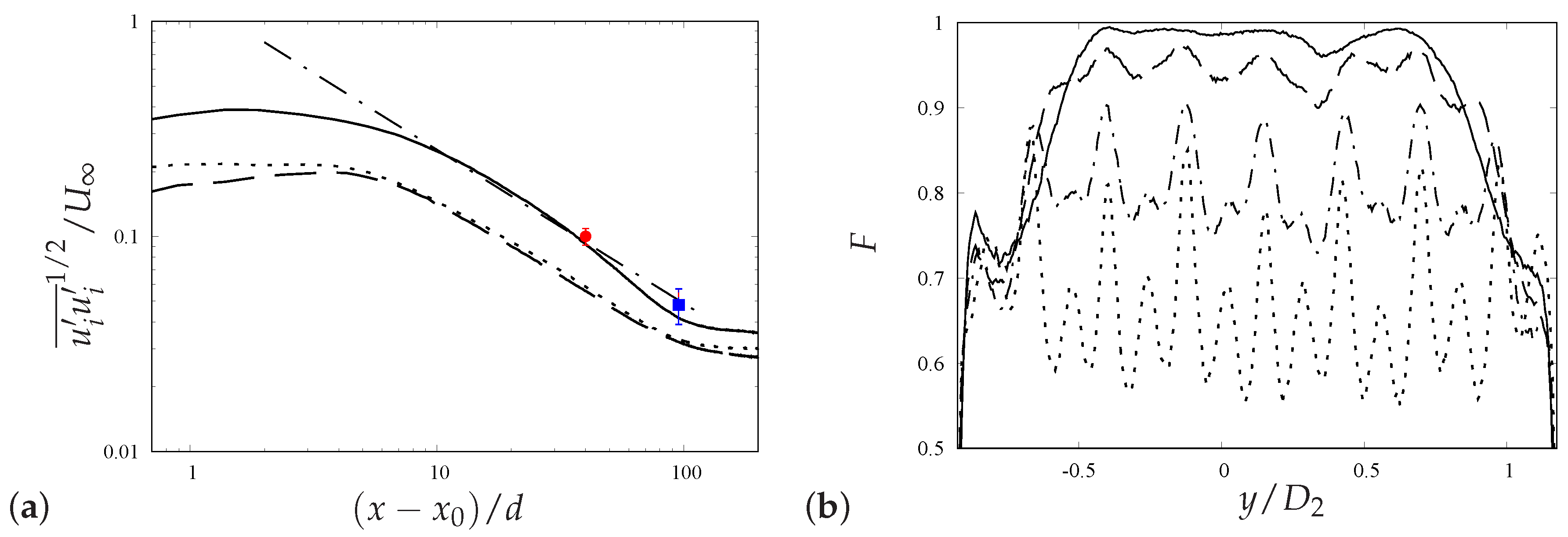
Figure 5.
Color contours of time-averaged streamwise velocity, normalized with the reference velocity , in the vertical plane passing through the tower axes: (a) no grid; (b) uniform grid; (c) non-uniform grid.
Figure 5.
Color contours of time-averaged streamwise velocity, normalized with the reference velocity , in the vertical plane passing through the tower axes: (a) no grid; (b) uniform grid; (c) non-uniform grid.

Figure 6.
Rotor-averaged streamwise velocity as funtion of the streamwise direction: ![Energies 10 00821 i009]() no grid,
no grid, ![Energies 10 00821 i010]() uniform grid,
uniform grid, ![Energies 10 00821 i011]() non-uniform grid. The vertical lines (
non-uniform grid. The vertical lines ( ![Energies 10 00821 i012]() ) denote the location of the grid and of the turbines.
) denote the location of the grid and of the turbines.
 no grid,
  uniform grid,
  non-uniform grid. The vertical lines (
  ) denote the location of the grid and of the turbines.
Figure 6.
Rotor-averaged streamwise velocity as funtion of the streamwise direction: ![Energies 10 00821 i009]() no grid,
no grid, ![Energies 10 00821 i010]() uniform grid,
uniform grid, ![Energies 10 00821 i011]() non-uniform grid. The vertical lines (
non-uniform grid. The vertical lines ( ![Energies 10 00821 i012]() ) denote the location of the grid and of the turbines.
) denote the location of the grid and of the turbines.
no grid, uniform grid, non-uniform grid. The vertical lines ( ) denote the location of the grid and of the turbines.
Figure 7.
Velocity profiles along the spanwise direction at hub height at different streamwise locations: ![Energies 10 00821 i013]() no grid,
no grid, ![Energies 10 00821 i014]() uniform grid,
uniform grid, ![Energies 10 00821 i015]() non-uniform grid; (a) ( upstream of the first turbine); (b) ( downstream of the first turbine); (c) ( downstream of the first turbine); (d) ( downstream of the second turbine).
non-uniform grid; (a) ( upstream of the first turbine); (b) ( downstream of the first turbine); (c) ( downstream of the first turbine); (d) ( downstream of the second turbine).
 no grid,
  uniform grid,
  non-uniform grid; (a) ( upstream of the first turbine); (b) ( downstream of the first turbine); (c) ( downstream of the first turbine); (d) ( downstream of the second turbine).
Figure 7.
Velocity profiles along the spanwise direction at hub height at different streamwise locations: ![Energies 10 00821 i013]() no grid,
no grid, ![Energies 10 00821 i014]() uniform grid,
uniform grid, ![Energies 10 00821 i015]() non-uniform grid; (a) ( upstream of the first turbine); (b) ( downstream of the first turbine); (c) ( downstream of the first turbine); (d) ( downstream of the second turbine).
non-uniform grid; (a) ( upstream of the first turbine); (b) ( downstream of the first turbine); (c) ( downstream of the first turbine); (d) ( downstream of the second turbine).
no grid, uniform grid, non-uniform grid; (a) ( upstream of the first turbine); (b) ( downstream of the first turbine); (c) ( downstream of the first turbine); (d) ( downstream of the second turbine).
Figure 8.
Time-averaged streamwise velocity profiles at hub height downstream of the first turbine. Exp. Data (•); -model RADM ( ![Energies 10 00821 i016]() ); Smagorinsky RADM (
); Smagorinsky RADM ( ![Energies 10 00821 i017]() ); Smagorinsky ALM (
); Smagorinsky ALM ( ![Energies 10 00821 i018]() ); Smagorinsky ALM (
); Smagorinsky ALM ( ![Energies 10 00821 i019]() ). (a) No grid; (b) uniform grid; (c) non-uniform grid.
). (a) No grid; (b) uniform grid; (c) non-uniform grid.
 ); Smagorinsky RADM (
  ); Smagorinsky ALM (
  ); Smagorinsky ALM (
  ). (a) No grid; (b) uniform grid; (c) non-uniform grid.
Figure 8.
Time-averaged streamwise velocity profiles at hub height downstream of the first turbine. Exp. Data (•); -model RADM ( ![Energies 10 00821 i016]() ); Smagorinsky RADM (
); Smagorinsky RADM ( ![Energies 10 00821 i017]() ); Smagorinsky ALM (
); Smagorinsky ALM ( ![Energies 10 00821 i018]() ); Smagorinsky ALM (
); Smagorinsky ALM ( ![Energies 10 00821 i019]() ). (a) No grid; (b) uniform grid; (c) non-uniform grid.
). (a) No grid; (b) uniform grid; (c) non-uniform grid.
); Smagorinsky RADM ( ); Smagorinsky ALM ( ); Smagorinsky ALM ( ). (a) No grid; (b) uniform grid; (c) non-uniform grid.
Figure 9.
TKE in the horizontal plane at hub height: (a) no grid; (b) uniform grid; (c) non-uniform grid.
Figure 9.
TKE in the horizontal plane at hub height: (a) no grid; (b) uniform grid; (c) non-uniform grid.

Figure 10.
Turbulent kinetic energy (TKE) profiles at hub height downstream of the first turbine. Exp. Data (•); -model RADM ( ![Energies 10 00821 i020]() ); Smagorinsky RADM (
); Smagorinsky RADM ( ![Energies 10 00821 i021]() ); Smagorinsky ALM (
); Smagorinsky ALM ( ![Energies 10 00821 i022]() ); Smagorinsky ALM (
); Smagorinsky ALM ( ![Energies 10 00821 i023]() ). (a) No grid; (b) uniform grid; (c) non-uniform grid.
). (a) No grid; (b) uniform grid; (c) non-uniform grid.
 ); Smagorinsky RADM (
  ); Smagorinsky ALM (
  ); Smagorinsky ALM (
  ). (a) No grid; (b) uniform grid; (c) non-uniform grid.
Figure 10.
Turbulent kinetic energy (TKE) profiles at hub height downstream of the first turbine. Exp. Data (•); -model RADM ( ![Energies 10 00821 i020]() ); Smagorinsky RADM (
); Smagorinsky RADM ( ![Energies 10 00821 i021]() ); Smagorinsky ALM (
); Smagorinsky ALM ( ![Energies 10 00821 i022]() ); Smagorinsky ALM (
); Smagorinsky ALM ( ![Energies 10 00821 i023]() ). (a) No grid; (b) uniform grid; (c) non-uniform grid.
). (a) No grid; (b) uniform grid; (c) non-uniform grid.
); Smagorinsky RADM ( ); Smagorinsky ALM ( ); Smagorinsky ALM ( ). (a) No grid; (b) uniform grid; (c) non-uniform grid.
Figure 11.
Iso-surfaces of phase-averaged vorticity magnitude superimposed to color contours of phase-averaged spanwise vorticity in the vertical plane through the tower axes: (a) no grid; (b) non-uniform grid. The phase-average is computed by sampling those instants for which one of the blades of the first turbine is in the vertical position pointing towards the tunnel ceiling; see Equation (21).

Figure 12.
Same as Figure 11, but the phase-average is now computed using the time instants when a blade of the second turbine is vertical and pointing upwards. Iso-surfaces: phase-averaged vorticity magnitude: . Color contours: spanwise component in the vertical plane through the tower axes. (a) No grid; (b) non-uniform grid.

Figure 13.
Performances: (a) power and (b) thrust coefficients of the the two wind turbines for the no-grid case (■), uniform grid case (•), and non-uniform grid case (▲). Open symbols, experiment; solid symbols, LES: RADM, Smagorinsky ; RADM, -model ; ALM, Smagorinsky ; ALM, Smagorinsky .
Figure 13.
Performances: (a) power and (b) thrust coefficients of the the two wind turbines for the no-grid case (■), uniform grid case (•), and non-uniform grid case (▲). Open symbols, experiment; solid symbols, LES: RADM, Smagorinsky ; RADM, -model ; ALM, Smagorinsky ; ALM, Smagorinsky .

Figure 14.
Time-averaged angle of attack along the blade span: ![Energies 10 00821 i024]() no grid,
no grid, ![Energies 10 00821 i025]() uniform grid,
uniform grid, ![Energies 10 00821 i026]() non-uniform grid; (a) first turbine; (b) second turbine.
non-uniform grid; (a) first turbine; (b) second turbine.
 no grid,
  uniform grid,
  non-uniform grid; (a) first turbine; (b) second turbine.
Figure 14.
Time-averaged angle of attack along the blade span: ![Energies 10 00821 i024]() no grid,
no grid, ![Energies 10 00821 i025]() uniform grid,
uniform grid, ![Energies 10 00821 i026]() non-uniform grid; (a) first turbine; (b) second turbine.
non-uniform grid; (a) first turbine; (b) second turbine.
no grid, uniform grid, non-uniform grid; (a) first turbine; (b) second turbine.
Figure 15.
RMS angle of attack fluctuation along the blade span: ![Energies 10 00821 i027]() no grid,
no grid, ![Energies 10 00821 i028]() uniform grid,
uniform grid, ![Energies 10 00821 i029]() non-uniform grid; (a) first turbine; (b) second turbine.
non-uniform grid; (a) first turbine; (b) second turbine.
 no grid,
  uniform grid,
  non-uniform grid; (a) first turbine; (b) second turbine.
Figure 15.
RMS angle of attack fluctuation along the blade span: ![Energies 10 00821 i027]() no grid,
no grid, ![Energies 10 00821 i028]() uniform grid,
uniform grid, ![Energies 10 00821 i029]() non-uniform grid; (a) first turbine; (b) second turbine.
non-uniform grid; (a) first turbine; (b) second turbine.
no grid, uniform grid, non-uniform grid; (a) first turbine; (b) second turbine.
Figure 16.
Thrust force damage equivalent load (DEL) for the (a) first and (b) second turbine: ■ no grid; ☐ uniform grid; ⧅ non-uniform grid.
Figure 16.
Thrust force damage equivalent load (DEL) for the (a) first and (b) second turbine: ■ no grid; ☐ uniform grid; ⧅ non-uniform grid.

Figure 17.
Power spectral density of the power production of the (a) first and (b) second wind turbine: ![Energies 10 00821 i030]() no grid case;
no grid case; ![Energies 10 00821 i031]() non-uniform grid;
non-uniform grid; ![Energies 10 00821 i032]() slope. The vertical lines indicate three times the rotational frequency of the first (
slope. The vertical lines indicate three times the rotational frequency of the first ( ![Energies 10 00821 i033]() ) and second (
) and second ( ![Energies 10 00821 i034]() ) turbine.
) turbine.
 no grid case;
  non-uniform grid;
  slope. The vertical lines indicate three times the rotational frequency of the first (
  ) and second (
  ) turbine.
Figure 17.
Power spectral density of the power production of the (a) first and (b) second wind turbine: ![Energies 10 00821 i030]() no grid case;
no grid case; ![Energies 10 00821 i031]() non-uniform grid;
non-uniform grid; ![Energies 10 00821 i032]() slope. The vertical lines indicate three times the rotational frequency of the first (
slope. The vertical lines indicate three times the rotational frequency of the first ( ![Energies 10 00821 i033]() ) and second (
) and second ( ![Energies 10 00821 i034]() ) turbine.
) turbine.
no grid case; non-uniform grid; slope. The vertical lines indicate three times the rotational frequency of the first ( ) and second ( ) turbine.

Table 1.
Large-eddy simulations (LES) parameters: sub-grid scale (SGS) model and rotor model.
| SGS Model | Model Constant | Rotor Model |
|---|---|---|
| -model | RADM | |
| Smagorinsky | RADM | |
| Smagorinsky | ALM | |
| Smagorinsky | ALM |
© 2017 by the authors. Licensee MDPI, Basel, Switzerland. This article is an open access article distributed under the terms and conditions of the Creative Commons Attribution (CC BY) license (http://creativecommons.org/licenses/by/4.0/).
Share and Cite
MDPI and ACS Style
Ciri, U.; Petrolo, G.; Salvetti, M.V.; Leonardi, S. Large-Eddy Simulations of Two In-Line Turbines in a Wind Tunnel with Different Inflow Conditions. Energies 2017, 10, 821. https://doi.org/10.3390/en10060821
AMA Style
Ciri U, Petrolo G, Salvetti MV, Leonardi S. Large-Eddy Simulations of Two In-Line Turbines in a Wind Tunnel with Different Inflow Conditions. Energies. 2017; 10(6):821. https://doi.org/10.3390/en10060821
Chicago/Turabian StyleCiri, Umberto, Giovandomenico Petrolo, Maria Vittoria Salvetti, and Stefano Leonardi. 2017. "Large-Eddy Simulations of Two In-Line Turbines in a Wind Tunnel with Different Inflow Conditions" Energies 10, no. 6: 821. https://doi.org/10.3390/en10060821
Note that from the first issue of 2016, this journal uses article numbers instead of page numbers. See further details here.