Multi-Objective Optimization of Building Energy Design to Reconcile Collective and Private Perspectives: CO2-eq vs. Discounted Payback Time


1
Department of Civil and Environmental Engineering, Norwegian University of Science and Technology, Byggteknisk, 2-236, Gløshaugen, Høgskoleringen 7A, Trondheim 7491, Norway
2
Department of Mechanical Power Engineering, Helwan University, Cairo 11790, Egypt
3
Department of Industrial Engineering, Università degli studi di Napoli Federico II, Piazzale Tecchio 80, Naples 80125, Italy
*
Author to whom correspondence should be addressed.
Energies 2017, 10(7), 1016; https://doi.org/10.3390/en10071016
Submission received: 22 May 2017
/
Revised: 26 June 2017
/
Accepted: 6 July 2017
/
Published: 18 July 2017
(This article belongs to the Special Issue Zero-Carbon Buildings)
Abstract
:Building energy design is a multi-objective optimization problem where collective and private perspectives conflict each other. For instance, whereas the collectivity pursues the minimization of environmental impact, the private pursues the maximization of financial viability. Solving such trade-off design problems usually involves a big computational cost for exploring a huge solution domain including a large number of design options. To reduce that computational cost, a bi-objective simulation-based optimization algorithm, developed in a previous study, is applied in the present investigation. The algorithm is implemented for minimizing the CO2-eq emissions and the discounted payback time (DPB) of a single-family house in cold climate, where 13,456 design solutions including building envelope and heating system options are explored and compared to a predefined reference case. The whole building life is considered by assuming a calculation period of 30 years. The results show that the type of heating system significantly affects energy performance; notably, the ground source heat pump leads to the highest reduction in CO2-eq emissions, around 1300 kgCO2-eq/m2, with 17 year DPB; the oil fire boiler can provide the lowest DPB, equal to 8.5 years, with 850 kgCO2-eq/m2 reduction. In addition, it is shown that using too high levels of thermal insulation is not an effective solution as it causes unacceptable levels of summertime overheating. Finally a multi-objective decision making approach is proposed in order to enable the stakeholders to choice among the optimal solutions according to the weight given to each objective, and thus to each perspective.
1. Introduction
During the last two decades, world primary energy consumption and carbon dioxide equivalent (CO2-eq) emissions have grown by around 50% and 40% [1], respectively, thereby raising increasing concerns over supply difficulties, exhaustion of energy resources and heavy environmental impacts (e.g., ozone layer depletion, global warming, climate change). In this framework, buildings account for about 40% of global energy uses in Europe and 32% in the World [2], and thus they are responsible for similar shares of associated polluting emissions. Therefore, it is clear that the optimization of building energy design is fundamental to face some crucial issues of present and future society, such as environmental pollution, climate change, energy poverty and economic crisis [3]. These issues are linked to two main actors that are interested in building energy performance, namely the collectivity (i.e., the public administration) and the private (i.e., the common citizen). The objectives of such actors are different and, often, divergent. Generally, the collectivity pursues the minimization of environmental impact, whereas the private pursues the maximization of financial viability. Furthermore, the proper building energy design requires to explore a huge domain of possible scenarios. Finally, it requires to solve complex multi-objective optimization problems with several design variables. Recent scientific literature offers several approaches to address such problems as shown in Section 1.1, where the focus is on Finnish case studies (see Section 1.1.1) because the current paper investigates the energy design of a residential building located in Finland. Finally, Section 1.2 elucidates aim and originality of the proposed study.
1.1. Optimization of Building Energy Design: Literature Review
Optimizing building energy design means to find the values of some design variables, related to the thermal characteristics of building envelope and/or to the types and operation schedules of energy systems, that minimize (or maximize) one or more objective functions. Generally, the possible combinations of these variables are considerable, and thus a robust optimization procedure requires to explore a wide domain of design scenarios. For each scenario, the values of the objective functions have to be reliably assessed in order to achieve worthy outcomes. To this end, proper building energy performance simulation tools, such as EnergyPlus [4], TRNSYS [5], ESP-r [6] and IDA ICE [7], have to be used. These tools perform transient energy simulations over typical years and produce reliable outcomes if the energy models are properly built and calibrated. Clearly, the computational times are not negligible being of the order of magnitude of some minutes for each simulation, depending on the building complexity. Definitely, not all possible design scenarios can be investigated by means of exhaustive researches because this would require prohibitive computational burden, and therefore the use of proper optimization algorithms is necessary. Several algorithms are available and they can be distinguished in [8] derivate-based and derivative-free ones, deterministic and stochastic ones, single-objective and multi-objective ones. The dominant algorithms for the optimization of building energy design are derivative-free, stochastic heuristic, multi-objective ones, such as genetic algorithms (GAs) [9]. This occurs for the following reasons:
- generally, the objective functions are not differentiable because they are black box functions provided, as output, by the mentioned simulation tools; therefore, only derivative-free algorithms can be used;
- stochastic heuristic algorithms are preferred because they ensure good sub-optimal solutions in reasonable computational times; in this regard, deterministic algorithms are, normally, not-effective because they require too many simulations (i.e., excessive computational times) to achieve slight improvements of the solutions;
In very recent years, several derivative-free, stochastic heuristic, multi-objective approaches for building energy design were proposed, as outlined by comprehensive review studies [14,15,16,17]. Most of these approaches were based on Pareto optimization [8] thereby aiming at the achievement of the Pareto front, that is the set of non-dominated solutions, which represent trade-off solutions among contrasting objective functions. For instance, in various studies [9,10,11,12,13], the same authors developed multi-objective optimization frameworks pursuing different aims. In [9,10,11], the GA algorithm provided by the optimization toolbox of MATLAB® (function “gamultiobj”) [18] was coupled with EnergyPlus and implemented for:
- optimizing building energy design combined with the model predictive control of HVAC (heating, ventilating and air conditioning) systems [9];
- identifying the optimal mix of renewable energy sources at the building level by minimizing primary energy consumption and investment cost [10];
- addressing building energy retrofit by minimizing thermal discomfort and primary energy consumption in order to find comfortable, energy-efficient and cost-effective solutions for different values of the available economic budget [11].
In [12,13], the mentioned GA was modified in order to reduce the required computational time and increase, at the same time, the robustness of optimal solutions. This algorithm was coupled with IDA ICE and employed to find low-emission, cost-effective design solutions for a Finnish dwelling [12]. Furthermore, the same GA was integrated within a comprehensive multi-stage optimization framework for cost-optimal and nearly zero-energy building solutions by considering as objective functions the minimization of primary energy consumption and lifecycle costs [13]. Notably, in this study, the GA was developed further to speed up the optimization process by avoiding unnecessary time consuming simulations and using post-processing when possible. Delgarm et al. [19] provided a new methodology, based on multi-objective artificial bee colony (MOABC), to optimize the design of building envelope by minimizing electricity consumption and thermal discomfort. The same aim was pursued by Yang et al. [20], who proposed a GA-based framework (denoted as MOPBEM) in order to minimize envelope construction cost, energy load and maximize window opening rate. Bre et al. [21] addressed the design optimization of a residential building by performing sensitivity analysis to screen the design variables and a GA to minimize energy consumption and discomfort hours. A GA was employed also by Brunelli et al. [22] for achieving sustainable design by setting five objectives: minimization of thermal energy demand, electric energy consumption and CO2-eq emissions as well as maximization of investment net present value (NPV) and thermal comfort. In the same vein, Fan and Xia [23] implemented a GA to address building envelope energy retrofit by considering both primary energy consumption and economic benefits (NPV and payback period). A weighted sum method was used to convert the multi-objective problem to a single-objective one. Similar objective functions were considered by Salata et al. [24] in order to compare the energy-efficiency and cost-effectiveness of different retrofit solutions for space heating and domestic hot water production. Kerdan et al. [25] developed a further simulation framework for building energy retrofit analysis and design optimization, denoted as ExRET-Opt, which allows to consider different objective functions, related to energy, exergy, economic, environmental and thermal comfort performance. Wu et al. [26] also addressed the issue of building retrofits by using a multi-objective optimization framework with the aim of reducing both lifecycle costs and CO2-eq emissions. Ascione et al. [27,28,29,30] developed a GA-based multi-stage and multi-objective framework to find cost-optimal and energy-efficient solutions concerning building design and/or retrofit. Thus, the main objective functions to be minimized were energy demands and global costs. This framework was applied to a complex reference hospital building [27] as well as to office [28], educational [29] and residential [30] buildings by considering the reduction of thermal discomfort too. Similarly, Mostavi et al. [31] proposed a comprehensive multi-objective framework to optimize building energy performance by minimizing lifecycle costs and polluting emissions while maximizing occupants’ thermal satisfaction. Finally, further recent studies, about design optimization, aimed at the minimization of objective functions related to lighting performance, such as electricity demand for artificial lighting [32] and visual discomfort [33].
1.1.1. Finnish Case Studies
Building energy needs for heating and electricity are responsible for about 30% of Finnish CO2-eq emissions [34], and thus the optimization of building energy performance can provide high potential environmental and economic benefits in Finland. In this regard, until few years ago, Finnish building regulations established that energy performance classes were based on thermal energy demand for space heating per unit of floor area. The classes addressed the energy efficiency of building envelope, heat recovery systems and heating terminals. However, they did not take account of primary energy systems as well as of the possible exploitation of renewable energy sources (RESs). Such lack of energy performance regulations in terms of specific annual primary energy or CO2-eq emission requirements together with the Finnish energy costs, which are among the lowest in the EU, led to the following drawbacks [35]: (1) electrical heating, which has the highest CO2 footprint, is widely used in the residential sector; (2) relatively low-efficient heat recovery systems and fans are used. In other words, the current Finnish building stock ensures good energy performance as concerns thermal energy demands but energy measures are necessary to reduce polluting emissions and achieve low-carbon buildings.
In this frame, in 2006 the VTT’s Energy renovation technologies project investigated the profitability of energy retrofit measures for three different building types [34], without any environmental estimations. In the same vein, Pylsy and Kalema [36] conducted a comprehensive sensitivity analysis in order to achieve low-energy cost-effective concepts for single-family houses in Finland. They assessed the impact on primary energy consumption of sundry options for insulation thickness, window type, building tightness, and efficiency of heat recovery as well as primary heating systems. However, no optimization procedures were implemented. Diversely, Hasan et al. [37] performed a mono-objective optimization in order to find the optimal combination of energy measures (e.g., additional thermal insulation, better window type, higher efficiency heating recovery type) for the minimization of lifecycle costs. Different economic assumptions were considered, but only one heating system was addressed. On the other hand, Alanne et al. [38] investigated the selection of a residential energy supply system as a multi-criteria decision-making problem involving both financial and environmental issues. They showed that micro-CHP (combined heating and power) systems are an effective alternative to traditional ones, especially from the environmental point of view. Finally, Hamdy et al. [12,39] proposed a GA-based multi-objective optimization approach combined with IDAICE (a building performance simulation program) in order to minimize CO2-eq emissions (related to heating energy consumption) and investment cost for a two-storey residential building. The type of primary heating system was addressed as a design variable besides the ventilation heat recovery type and six building envelope parameters: level of building tightness, insulation thickness of the external wall, floor and roof, type of window glazing and window shading. The main conclusions of the study were the following:
- the optimization can produce up to 32% reduction in CO2-eq emissions and up to 26% saving in investment cost;
- the influence of the thermal insulation level of the building envelope on energy performance can be reduced into an overall building U-value (Ubldg);
- too low values of to Ubldg imply the need of ventilation measures or shading options in order to avoid summer overheating.
The energy design of same building is investigated in the current study but with a different multi-objective optimization approach, which better addresses and conciliates collective and private perspectives.
1.2. Aim and Originality of This Study
It is clear that the optimization of building energy design can involve several objective functions as shown by the above literature review. These objectives are linked to the two aforementioned main perspectives that are in conflict in building energy performance, namely the collective and the private ones. Thus, which are the most proper objective functions in order to represent these two perspectives? The collectivity (i.e., the public administration) aims at minimizing the environmental impact of the building sector in order to achieve national and international targets concerning low-carbon societies and sustainable development. On the other hand, the private (i.e., the common citizen) aims at maximizing the financial viability of the investment, and thus it is particularly interested in the time that is needed to achieve an economic profit. Therefore, this study assumes that the most representative objective for the collectivity is the minimization of carbon dioxide equivalent (CO2-eq) emissions, whereas for the private is the minimization of the discounted payback time. The time value of money is evaluated considering interest, inflation, and energy price escalation rates. In order to address the described two objective functions, a GA-based bi-objective optimization approach is proposed. This allows to achieve an original aim, that is identifying Pareto trade-off solutions, concerning building energy design, that reconcile collective and private perspectives. Since low-carbon designs, with high levels of thermal insulations, could lead to summertime overheating, a constraint is set on the maximum value of discomfort hours. It should be noticed that a bi-objective optimization is conducted because considering more than two objective functions is not recommended [11], since it would increase the computational burden as well as the complexity in outcomes’ interpretation.
The described optimization procedure is applied to the Finnish single-family dwelling located in the city of Helsinki investigated by the same authors in [12,39]. The same design variables for building energy design are considered, but a different approach is employed and a more comprehensive economic and environmental analysis is performed. In order to highlight the usefulness of the new approach, the achieved outcomes are compared with those of [12]. Notably, a single-family house is explored because, at the European Union (EU) level, the residential one is the building sector that causes the largest amount of CO2-eq emissions (i.e., higher 70%) and, within it, single-family houses represent the largest share, responsible for around 60% of CO2-eq emissions, equivalent to more than 400 Mt/a [40].
2. Methodology for the Optimization of Building Energy Design
The current study proposes a bi-objective optimization approach to address building energy design. The methodology is based on the coupling between a genetic algorithm and IDA Indoor Climate and Energy (IDA ICE) [7]. This latter is a whole-building dynamic performance simulation program that addresses all issues concerning building energy design (e.g., geometry, envelope, HVAC systems, operation, lighting, equipment). IDA ICE provides simultaneous dynamic simulations of heat transfer and air flows. It is a suitable and accurate tool for the simulation of thermal comfort, indoor air quality and energy consumption in complex buildings, since it has been validated for different case studies [41,42,43].
2.1. Formulation of the Optimization Problem
The optimization problem is formulated below:
subject to
where is the vector encoding the design variables.
F is the vector of the two objective functions to be minimized, which are the difference in CO2-eq compared to a reference design (i.e., dCO2_eq) and the discounted payback time (i.e., DPB), whereas x is a vector that encodes the design variables, which can be integers or continuous. Thus, a mixed integer optimization problem is handled. Finally, a constraint is set as regards thermal comfort by establishing a maximum acceptable value for , which is a performance indicator concerning discomfort hours and it is explained in Section 2.1.3.
2.1.1. Design Variables
The design variables concern building energy design and are encoded by the vector x. Therefore, they represent energy measures that can be related to:
- thermal insulation of building opaque (i.e., vertical walls, roof and floor);
- window type;
- shading type;
- building tightness level;
- heat recovery type;
- heating, ventilating and air conditioning (HVAC) system type;
- primary energy system type.
The number of design variables is indicated with N.
2.1.2. Objective Functions
The proposed optimization approach aims to conciliate collective and private perspectives by considering two objective functions that represent the mentioned perspectives as detailed in the following subsections. The final aim is to find low-emission and cost-effective design solutions for building design.
Collective Perspective: Minimization of CO2-eq Emissions
The minimization of CO2-eq emissions is chosen as objective function in order to represent the collective perspective. It allows to assess the environmental impact of the candidate solutions. The calculations consider the CO2-eq emissions (CO2-eq) related to heating energy consumption (during a lifespan of 30 years) and the CO2-eq emissions related to the embodied energies of thermal insulation volume and window type. The lifespan of 30 years is used as recommended by current EU regulations for lifecycle assessments concerning residential buildings [44,45]. For comparison purpose, the difference (dCO2-eqi) between the CO2-eq for any case (CO2-eqi) and that for the reference design (CO2-eqref) is calculated as shown in the following equations:
where the subscripts (energy, insulation, and window) denote the emission sources, Abldg is the building gross floor area. It is highlighted that compared to [12] a more comprehensive assessment of environmental impact is performed, since [12] considered only CO2-eq energy in the calculation of CO2-eq emissions.
The annual CO2-eq emissions related to heating energy consumption (CO2-eq energy) are calculated according to Equation (3) by using primary greenhouse gas emission factors (EFs) from [46]. The emission factors were evaluated for different types of energy (electrical, light oil, district heating) supplied to the buildings of Helsinki, Finland (i.e., the location of the investigated case study). The emission factors consider three major greenhouse gases: CO2, sulphur, and nitrogen:
where Q (kWh) is the annual heating energy (space heating, system heat loss, domestic hot water heating), EF is the primary greenhouse gas emission factor, and η is the average annual efficiency of the heating system. The annual heating energy Q is calculated by using IDA ICE.
The CO2-eq emissions related to embodied energies of insulation (CO2-eq insulation) are calculated considering embodied energies factors from [47]:
where the subscripts v, r and f refer to the thermal insulation of vertical external walls, roof and basement floor, respectively, A is the surface area, X is the insulation thickness, EE is embodied energies factor, EFelectricity is the primary greenhouse gas emission factor of electricity [46].
The CO2-eq emissions related to embodied energies of windows (CO2-eq window) are calculated considering embodied energies factors from [48]:
Aw is the window surface area and EEw is the embodied energy per window area.
Private Perspective: Minimization of the Discounted Payback Time
The minimization of the discounted payback time (DPB) is chosen as objective function in order to represent the private perspective. It allows one to assess the financial viability and cost-effectiveness of the candidate solutions compared to the reference design.
It is noticed that, for a fair cost comparison between any solution and the reference one, all relevant costs (i.e., investment, operating, maintenance and replacement costs) should be taken into consideration. Moreover, because of the time value of money, the costs have to be compared on similar basis with respect to time. In this regard, several approaches can be adopted for such cost comparisons, and the most common ones are net present value (NPV), annual costs and lifecycle savings (LCS) [49].
The lifecycle saving (LCS) approach considers the difference in the present value of the costs between the reference design and any solution and determines the conditions under which that solution is advantageous. The time at which the LCS becomes zero (then it gets positive) provides the discounted payback time (DPB). In this study, DPB is used to evaluate the cost-effectiveness of the candidate solutions. It takes account of interest, inflation, and energy price escalation rates, and it is calculated by using the trial and error technique assuming ±5 € LCS as a tolerance:
being:
where:
- LCC is the lifecycle cost, the subscribe ref denotes the reference design, the subscribe x denotes any candidate solution;
- re is the real interest rate including the effect of the escalation rate of energy prices;
- r is the real interest rate not including the effect of escalation rate of the energy prices;
- i is the interest rate and f is the inflation rate.
In order to calculate the lifecycle saving LCS, there is no need to determine the LCC for the whole building. Only the differences produced by the variation of specified parameters between the reference case and any candidate solution can be used:
where dIC (€) is the difference in the initial investment cost for specified items, dOC (€) is the difference in the operating cost, dSC (€) is the difference in the service cost, and dRC (€) is the difference in the replacement cost (other than the initial difference).
In particular, dIC (€) is the sum of the differences in the initial investment cost for the N energy measures, which are represented by the design variables:
dSC is the sum of the differences due to added costs for service of the heating system in the lifespan of 30 years (other than the initial difference):
where YMC is the yearly maintenance cost as a percentage of investment cost (ICsys) of heating system, αservice is the discount factor for the services assessed over n = 30 years:
dRC is the sum of the differences due to added costs for the replacement of energy measures with lifespan lower than 30 years:
where:
being RC’j the replacement cost (not discounted) of the j-th measure that is required after nj years. No residual values for the measures are considered for avoiding of overestimating the cost-effectiveness of the investments. Furthermore, as shown in Section 3.1, the investigated energy measures have lifespans equal to either 15 or 30 years, thus no residual values have to be considered.
dOC is the present value of the difference in heating energy consumption (i.e., space heating, system heat losses, and domestic hot water production):
where E is the annual energy consumption for total heating (kWh/a), penergy is the energy price [€/kWh], αenergy is the discount factor that takes into account the effect of inflation and escalation of energy price and it is calculated from [50] over n = 30 years:
From the previous equations, it is clear that DPB is a function of the rates of interest, inflation, and energy price escalation, in addition to the lifespan of the building. In this regard, the assumptions, made in the current work concerning economic (and also environmental) factors, are discussed in Section 3 where the investigated case study is detailed.
2.1.3. Constraint: Summertime Overheating
A constraint is set, i.e., DH24 ≤ DH24limit, in order to avoid excessive summertime overheating and to not overestimate the investment effectiveness. Indeed, the HVAC energy consumption (consequently the CO2-eq emissions) depends on the criterion of thermal comfort, i.e., disregarding the summer overheating makes feasible additional thermal insulation and thus higher energy savings for space heating. Therefore, in order to avoid this and to assess the level of summertime overheating, the parameter DH24 (degree hours) is used and defined as the summation of the operative temperature degrees higher than 24 °C in the warmest zone during a one-year simulation period (8760 h), as follows:
where:
where Ti is the operative temperature (°C) at the center of the warmest zone and Δt is one hour time period (h).
dH24 = (Ti − 24) · Δt when Ti − 24 > 0
dH24 = 0 when Ti − 24 ≤ 0
The current study addresses two levels of summertime overheating. P1 and P2 are used to denote the Pareto front of the two levels, respectively. The first level (P1) disregards the summer overheating, aiming at extreme optimal trade-off relation between the two objectives: minimum DPB and maximum CO2-eq reduction. The second level (P2) considered the degree-hours DH24 value of the reference design (DH24 = 2400 °C.h) as upper limit (i.e., DH24limit).
2.2. Optimization Procedure
The optimization problem is solved implementing a modified simulation-based genetic algorithm (GA), which was proposed by the authors in [12] and is run in MATLAB® environment (MATLAB®, MATrixLABoratory—7.10.0 [18]). GAs are derivative-free, stochastic, optimization algorithms that allow both mono- and multi-objective optimization. They carry out the “Darwinian” evolution of a population of individuals (i.e., solutions) through a series of iterations (denoted as generations) by means of the processes of selection, crossover, mutation and survival of the best individuals. Finally, they provide good sub-optimal solutions when a stop-criterion is satisfied, e.g., when a maximum number of generations is reached or the change in the optimal solutions between two next generations is lower than an established tolerance.
In particular, the employed GA is called PR_GA_RF and was proposed in [12] to which readers can refer for details. It derives from a variant of NSGA-II, which is a controlled elitist non-dominated sorting genetic algorithm developed by Deb et al. [51]. In this regard, NSGA-II is appropriate to solve multi-objective problems concerning building energy design with huge solution domains [9,10,11,27,28,29,30], but it could provide low performance when the number of iterations is too low [52]. Thus, when the performed iterations are not sufficient, the achieved sub-optimal solutions could be significantly far from the real Pareto front [27,52]. This is mainly due to the random behaviour of the algorithm and the inability to keep all non-dominated solutions throughout the optimization procedure. Indeed, through each generation, NSGA-II implements elitism by keeping two populations of size s, namely the adult generation P (deriving from the previous generation) and the “child” improved population Q, which originates from P by means of the processes of crossover and mutation. The individuals of Q are selected based on a non-domination Pareto concept. When the number of achieved non-dominated solutions exceed s, the algorithm screens such solutions based on a crowding distance measure in order to ensure high population diversity, which is fundamental to converge to the real Pareto front. Thus, some non-dominated solutions can be rejected and go wasted. Finally, NSGA-II could fail when the number of performed iterations is too low. In this regard, setting the proper number of maximum iterations is not trivial because the Pareto front is not known “a priori”. The issue can be solved by performing a large (even redundant) number of iterations, but, generally, this is not feasible for building optimization because the procedure would imply prohibitive computational times. Indeed, the assessment of the objective functions for each individual requires to run building simulation tools that usually need simulation times around minutes [27].
In this study, in order to improve the performance of NSGA-II reducing the described failing chances, a passive archiving strategy and two deterministic optimization phases are added, namely the preparation phase denoted with PR and the refine phase denoted with RF. Hence, the employed genetic algorithm is called PR_GA_RF [12]. The implementation of the cited deterministic phases reduces the risk of convergence to local optimal solutions [52]. The algorithm is run by using different function of the MATLAB® optimization toolbox. In particular, the initial preparation phase (i.e., PR) provides the GA with a good initial population of solutions, rather than a stochastic sample, by employing a single-objective sequential quadratic programming algorithm, i.e., the function “fmincon”. This latter allows to minimize one objective function assuming the other as a constraint. Different constraint values are considered and the minimization is performed three times, achieving a good initial population by sorting the individuals based on the concepts of non-domination and diversity. Then, the employed variant of NSGA-II [51] is implemented by launching the function “gamultiobj”. A passive archiving strategy is used in order to avoid losing non-dominated solutions. Finally, the refine phase (i.e., RF) is carried out by launching the function “fminmax” in order to yield optimal solutions, taken from the GA outcomes, to the utopia point. This allows to avoid a large number of inefficient GA generations, thereby reducing the needed computational time, as well as to obtain a higher number of optimal Pareto solutions.
2.2.1. Optimization Scheme
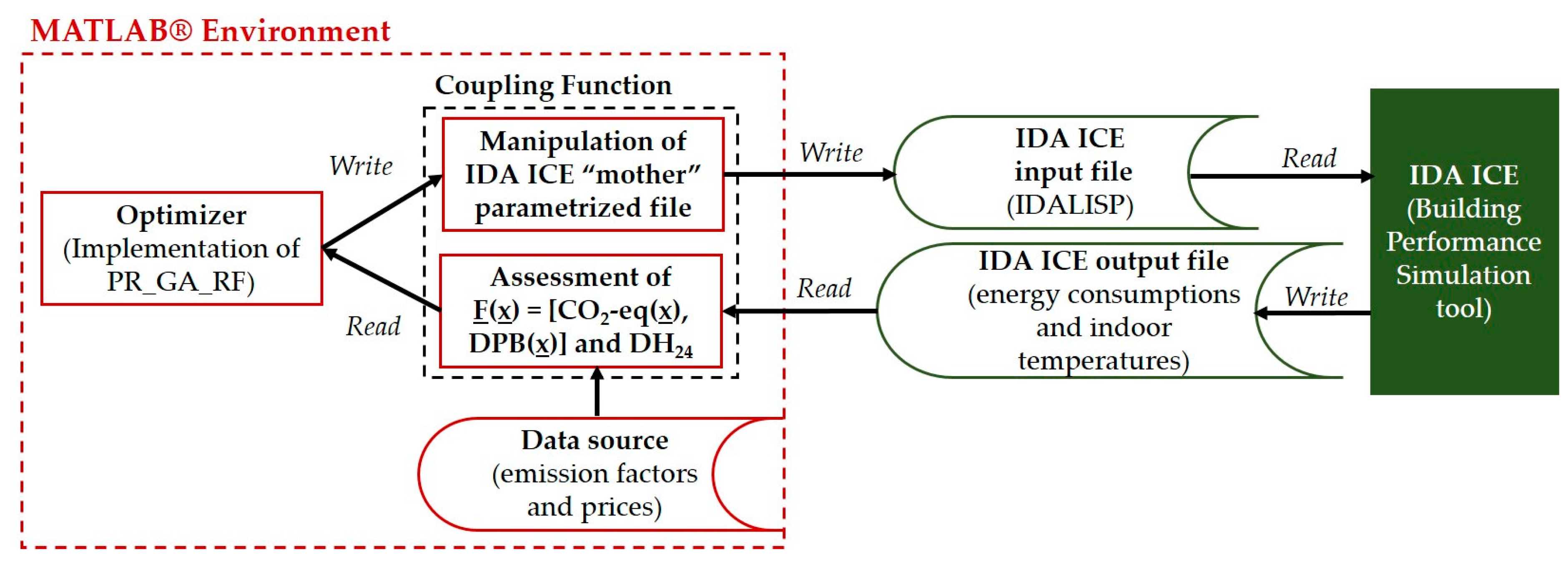
As shown in the previous subsection, all phases of the optimization algorithm PR_GA_RF are implemented under MATLAB® environment, whereas energy simulations are performed using the building performance simulation tool IDA ICE. Therefore, in order to couple MATLAB® and IDA ICE, a coupling function is written under MATLAB® environment. This function operates in two directions. On one hand, it converts the vector x of encoded design variables into an IDA ICE input file (IDALISP) by handling and manipulating a “mother” file that is parametrized. It is noticed that the vector x represents a generic energy design solution, i.e., an individual investigated by the GA. On the other hand, the coupling function converts the outputs of IDA ICE simulations, concerning energy consumptions and indoor temperatures, into the vector of objective functions F(x) = [dCO2-eq(x), DPB(x)] and the value of DH24, Therefore, the bi-directional communication between MATLAB® and IDA ICE is achieved. The described optimization scheme is proposed in Figure 1 and enables to consider any kind of discrete or continuous design variables linked to energy conservation measures that can be modeled in IDA ICE. Indeed, an proper parametrization of IDA ICE “mother” input file allows to take account of measures related to materials and thermal characteristics of the building envelope, to building use and operation (in particular occupant behavior), as well as to energy (in particular HVAC) systems. Only for example purposes, the thickness of a thermal insulation layer can be encoded in the “mother” file by a continuous parameter, to which a value is assigned by the coupling function based on x. Similarly, the heating system can be encoded by a discrete parameter, which can assume a limited set of integer values, each of them representing a plant configuration. Thus, the scheme can support the integration of the proposed robust framework for building energy optimization in comprehensive Building Information Modeling (BIM) platforms, since the described parametrization process enables to easily model and modify the main factors affecting building energy performance, from materials to systems. Definitely, this would support to handle the different design levels of development (i.e., LOD) as well as to simplify the communication among the different teams of experts involved in building design.
2.2.2. Comparison with Other Optimization Algorithms
The literature review of Section 1.1 shows that the most frequently used algorithms for the optimization of building energy design are definitely derivative-free, stochastic heuristic, multi-objective ones, such as the employed PR_GA_RF. They are simulation-based methods [8] and, in most cases, provide the Pareto front from which the final optimal solution is pick up by means of multi-criteria decision-making. As shown in [6,8,52], among these algorithms, the most proper ones for building energy optimization are: annealing, tabu search, ant colony, differential evolution, particle swarm and genetic algorithms (GAs). Indeed, they are designed to face highly complex optimisation problems, such as those concerning building design. In particular, recent years have seen an increasing interest in using GAs in order to optimize the main levers affecting building energy behaviour, namely envelope, operation and energy systems. In a literature review, Hamdy et al. [16] showed that the use frequency of GAs in recent building optimization studies is around 40%. This great diffusion is mainly due to the high performance of these algorithms with huge solution domains in terms of trade-off between outcome reliability and computational burden [27]. According to Deb [51], the variants of NSGA-II seem to be the most efficient GAs for complex multi-objective problems. Indeed, they were used in several studies addressing building design [9,10,11,12,13,20,21,27,28,29,30]. That is why a variant of NSGA-II is employed in this study. In addition, the original algorithm is modified by adding the deterministic preparation (PR) and refine phases (RF), as previously explained, in order to maximize the GA computational performance. Indeed, as argued in [12,52], the proposed multi-phase modified algorithm increases the robustness and reliability of the GA by speeding up, at the same time, the algorithm convergence. In other words, it ensures good sub-optimal (very close to optimal) solutions with a reasonable number of iterations. In this regard, in [16], the performance of a similar algorithm (i.e., the PR_GA) in addressing the design of a nearly-zero energy building was compared with the performance of other six algorithms. The comparison considered a controlled non-dominated sorting genetic algorithm with passive archive (pNSGA-II), a multi-objective particle swarm optimization (MOPSO), an elitist non-dominated sorting evolution strategy (ENSES), a multi-objective evolutionary algorithm based on the concept of epsilon dominance (evMOGA), a multi-objective differential evolution algorithm (spMODE-II), and a multi-objective dragonfly algorithm (MODA). Different indicators were investigated for the comparison, such as running time, convergence to a benchmarking optimal set, diversity and number of solutions of the Pareto front. The outcomes showed that the PR_GA provides the best trade-off among the examined performance indicators, thereby representing the best choice for building performance optimization. For this reason, a variant of PR_GA is here employed, and the refine phase is added in order to achieve a further reduction of computational times as well a higher number of optimal solutions.
3. Case Study: A Typical Finnish Dwelling
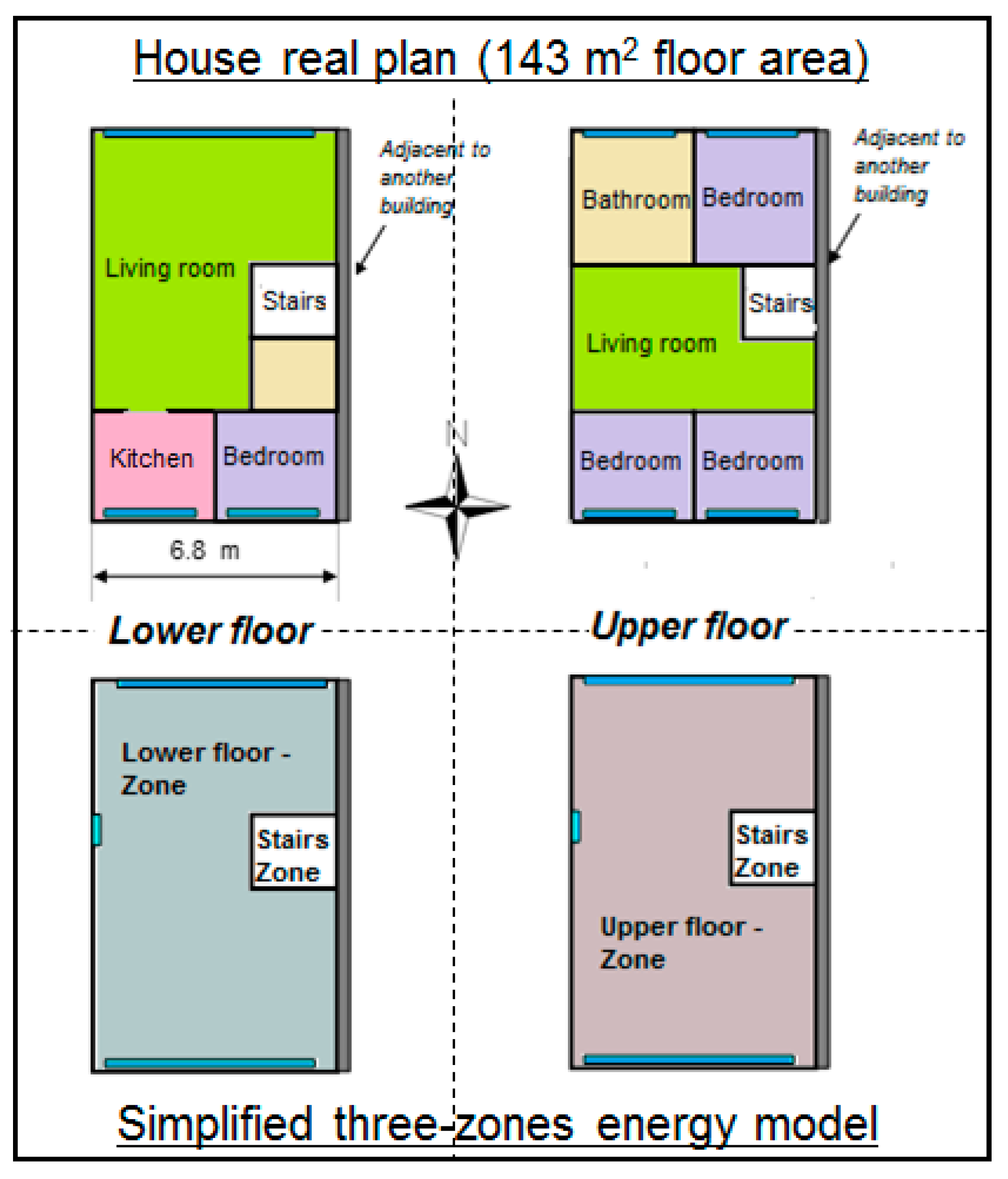
The methodology is applied to a typical Finnish two-storey dwelling, located in Helsinki, represented in Figure 2. The house gross floor area is 143 m2, the window surface is around 15% of the floor area, the internal height is 2.5 m for both storeys, which are connected by a staircase.
The energy design of the same case study was investigated by Hamdy et al. in [12] by means of a different optimization approach. Therefore, the same assumptions concerning building modeling, environmental and economic factors are made, as shown in Section 3.1, in order to compare the achieved outcomes with those of [12].
3.1. Assumptions Concerning Building Modeling, Environmental and Economic Factors
As concerns building energy modeling and analysis, IDA ICE simulations are performed by using Helsinki-Vantaa TRY2012 weather data file [53]. In order to reduce the simulation times, the dwelling is represented by means of a simplified building model (see Figure 2) with three (open plan) zones: lower floor, upper floor and staircase. On North and South exposures, a window is considered for each storey in order to achieve the total building windows’ surface (i.e., 20 m2). In addition, a small window (0.9 m2) is assumed at the middle of each storey with a special PI-controller for summer cooling purposes. In particular, these two small windows open proportionally when the outdoor temperature is lower than the indoor one and this latter is higher than 24 °C. This control logic aims to emulate the human behavior to open the window for improving thermal comfort in summertime by means of natural ventilation. The endogenous heat gains due to people, lighting and electric equipment are assumed as established by the Finnish building code D5-2007 [54] and set in IDA ICE simulations according to hourly schedules over the year. Concerning the HVAC systems, an air handling unit (AHU) supplies fresh air to bedrooms and living room and draws the exhaust air from bathrooms and kitchen to a cross air-to-air heat recovery system. The AHU supply air temperature is kept at 18 °C when the incoming outdoor air temperature is lower than this temperature. The average exhaust airflow from the house is equal to 0.65 air change per hour (ACH) (h−1), which is higher than the minimum level (0.5 h−1) required by the Finnish Building code D2-2003 [55]. All told, each IDA ICE simulation requires a computational time around 2 min by using a processor Intel® CoreTM i7 at 2.00 GHz.
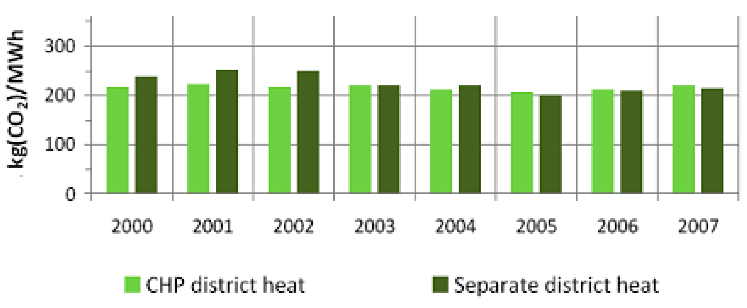
As concerns the environmental assumptions (see Section 2.1.2), the CO2-eq emissions related to heating energy consumption are calculated by using primary greenhouse gas emission factors (EF) from [46]. Although the continuous developing in energy-production technologies reduces the specific emissions, the current study assumes constant values of EF. Indeed, the Finnish statistics show that there is no significant variation in the specific CO2 emissions from district heating generation during the last decades (see for instance Figure 3 that refers to the period 2000–2007) [56].
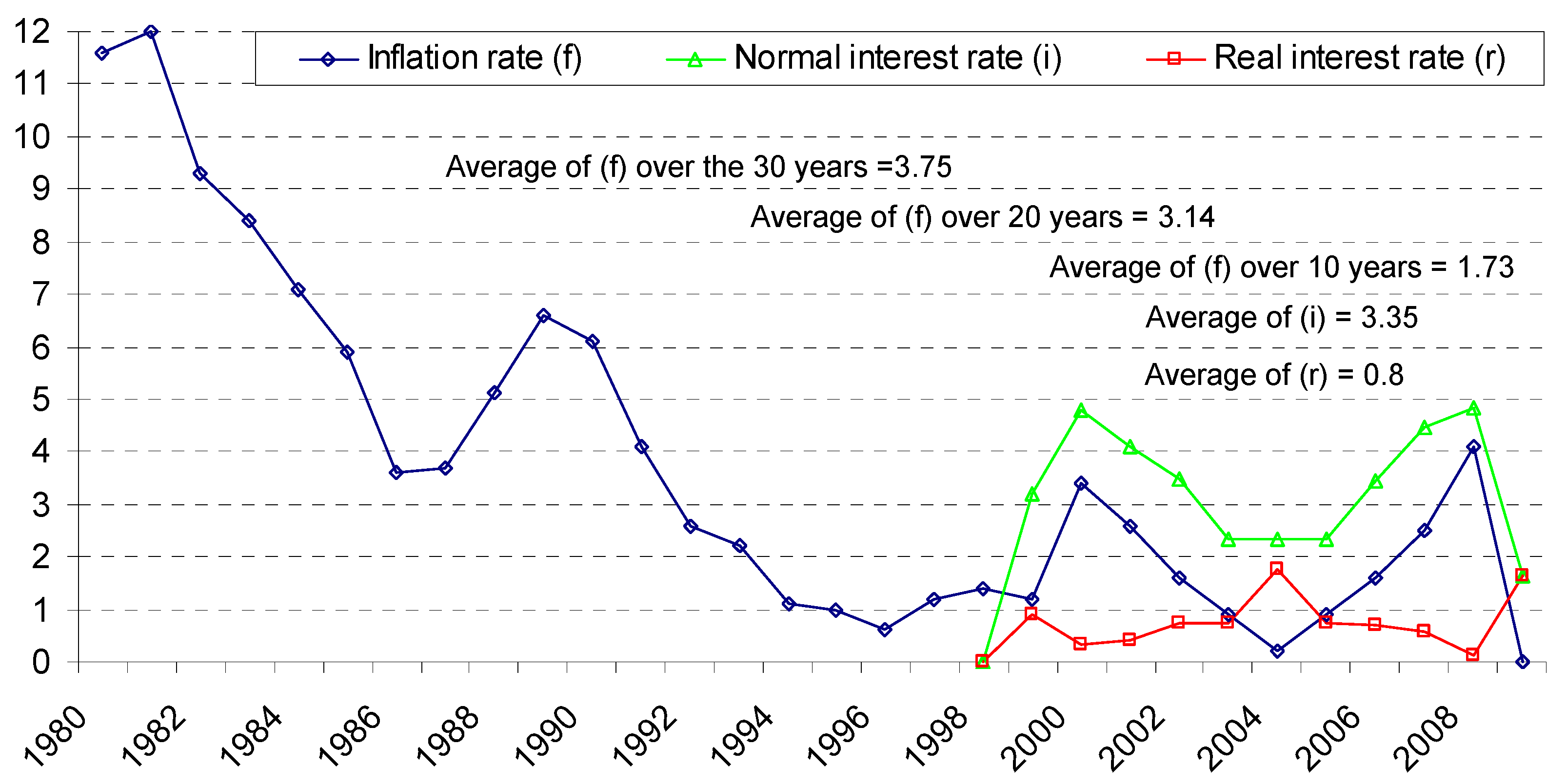
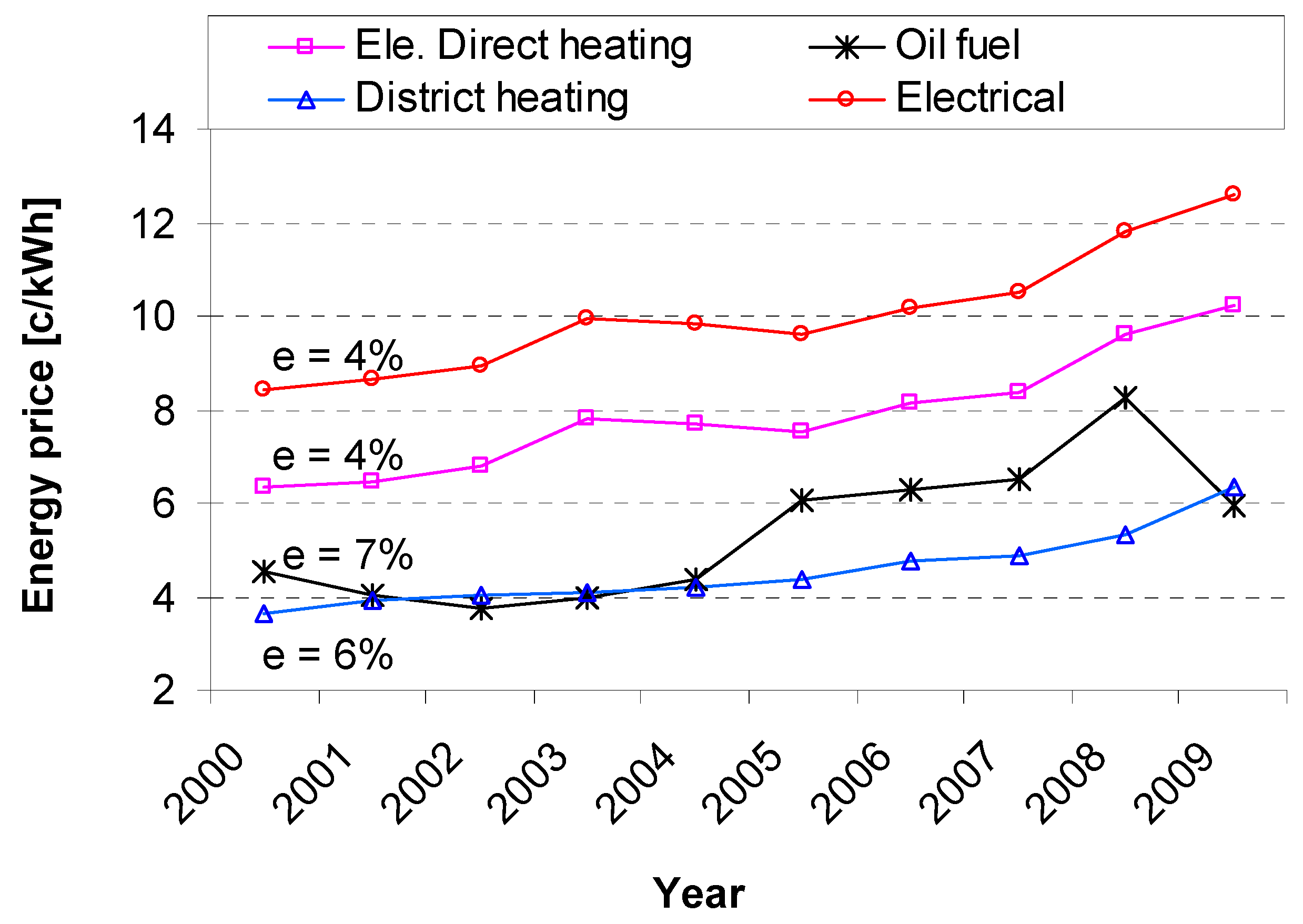
As concerns the economic assumptions, it should be noticed that different scientific studies, in the last years, addressed the economic impact of building energy design in Finland. In this regard, an important factor affecting the energy measures’ profitability is the real interest rate, which gives the increase in the buying power considering the effect of the inflation rate. Alanne et al. [38] addressed a range of real interest rates (from 2% to 6%), which were estimated based on market interest rates and the works of Manczyk [57] and Collins et al. [58]. Pylsy and Kalema [36] assumed a value equal to 3%. Hasan et al. [37] considered real interest rates of 2.94% and 4.9%, respectively, for two different investigated cases. Saari et al. [59] assumed 3% real interest rate, evaluating the payback period for a number of different energy saving design concepts for a typical house in Finland. In this frame, Figure 4 presents the normal interest rates, the inflation rates, and the real interest rates in the last years according to the Finnish statistics. Another important economic factor is the escalation rate of energy prices. In this regard, Figure 5 shows the energy price of direct electric heating, light oil, district heating, and electricity during the period from 2000 to 2009 in Finland.
All told, the discounted payback time is highly affected by the economic assumptions (real interest rate and energy price escalation rate). The literature shows that, during the last years, the energy price escalations of district heating and light oil are higher than the escalation of electricity price. The average value of the real interest rate (r) during the last ten years, in Finland, is around 1%. Hence, in the current study, two economic cases are investigated. The first case assumes high real interest rate (4%) and low energy price escalations 2%, 3.5%, 3%, and 2% for the four studied heating energy sources, i.e., direct electrical heating, oil fire boiler, district heating, and GSHP, respectively. The second case addresses lower real interest rate and higher energy price escalations (see Table 1). Case 2 is closer to the current economic situation in Finland.
3.2. Detailed Characterization of the Design Variables for Building Energy Design
The same design variables, and thus energy conservation measures, investigated in [12] are taken into account. In more detail, as concerns building envelope, thermal insulation of external vertical walls, roof and basement floor, window type, shading type as well as building tightness are taken into account. As concerns the HVAC system, ventilation heat recovery type and heating primary energy system are considered. These N = 8 design variables are detailed in the following Table 2, Table 3, Table 4, Table 5, Table 6, Table 7 and Table 8. Table 2 shows the reference values, lower and, upper bounds, as well as types (discrete or continuous) of the variables. Table 3, Table 4, Table 5, Table 6, Table 7 and Table 8 provide further details.
Heating systems are assumed oversized in order to ensure the minimum acceptable indoor temperature (21 ± 1 °C) for all building envelope solutions. The building tightness for the reference design (i.e., n50 = 4 h−1) is set according to the National Code of Finland D2-2003 [54]. The investment costs of energy measures as well as the energy prices are set equal to the values used in [12]. The lifespan of all energy measures is equal to the considered calculation period, i.e., 30 years, except for heat recovery systems that have a lifespan of 15 years (the replacement is taken into account during the investigated lifecycle).
4. Application to the Finnish Case Study: Results
The aim of the current work is to introduce low-emission cost-effective solutions for modern dwellings in the cold climate of Finland in order to conciliate collective and private perspectives. By implementing the described optimization approach (see Section 2), the environmental impact and the financial viability of 13,456 integrated building solutions are evaluated considering two cases with different economic assumptions (see Table 1). The 13,456 solutions consist of 3364 combinations among the first seven design variables (see Table 2, Table 3, Table 4, Table 5, Table 6 and Table 7) and the four considered heating systems (see Table 8).
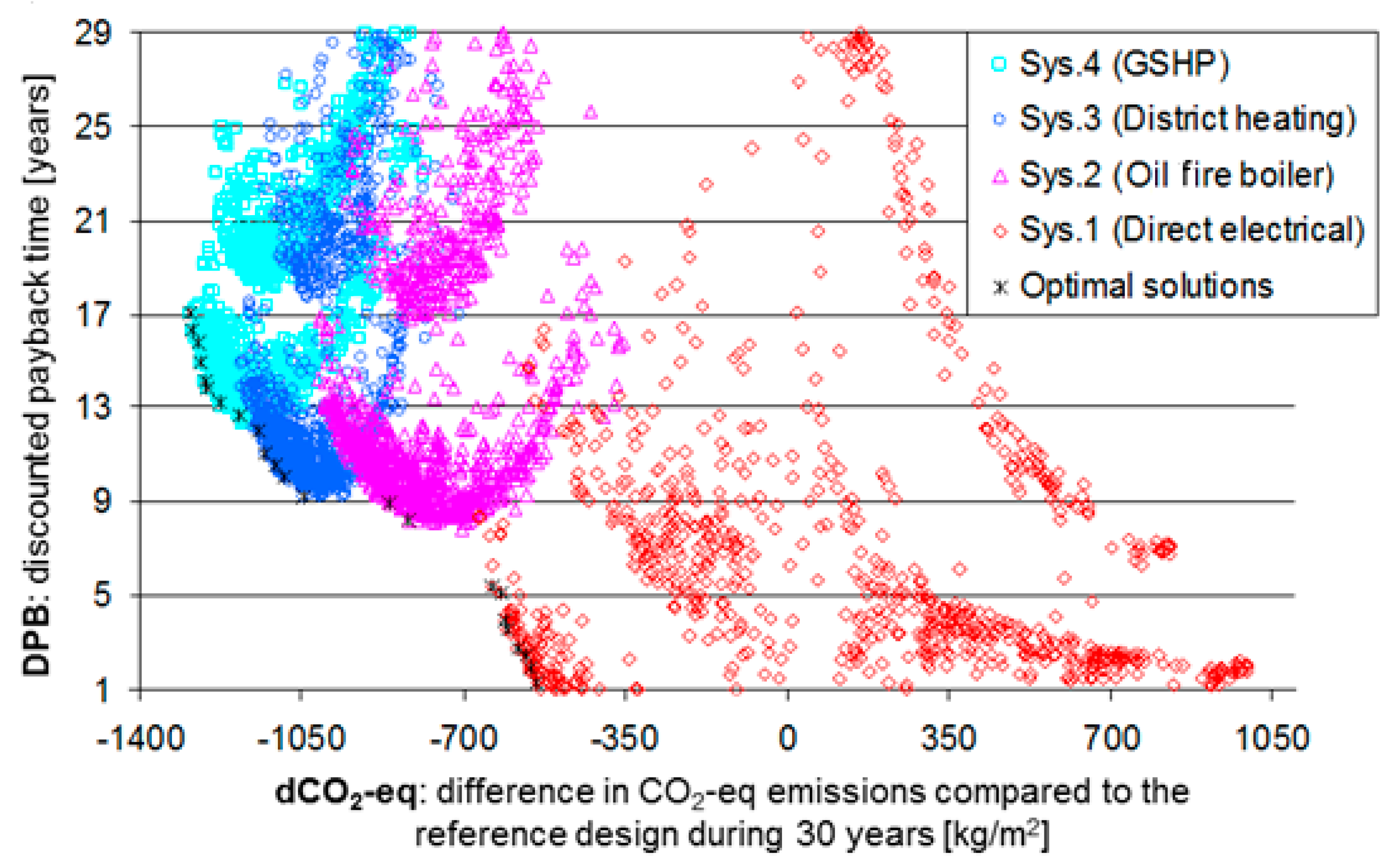
Figure 6 presents the main results achieved for Case 1 by showing the candidate solutions in terms of dCO2-eq and discounted payback time, DPB, (see Section 2.2) and classifying the solutions according to the heating energy source. In addition, the optimal solutions are highlighted on the front of the solution space, i.e., the Pareto front. These outcomes show that, during a lifespan of 30 years, the optimal solutions of the ground source heat pump (GSHP) can reduce the CO2-eq emissions by 1300 kg /m2 with a 17 year payback time or by 1180 kg /m2 with a 12.5 year payback time. Less reduction can be achieved by the district heating optimal solutions (i.e., 1150 kgCO2-eq /m2 with 12 year payback time or 1050 kgCO2-eq /m2 with 9.5 year payback time). The oil fire boiler can cut 850 kgCO2-eq/m2 with an 8.5 year payback time. If the reference design heating system (direct electrical heating) is not replaced at most 650 kgCO2-eq/m2 can be reduced by additional insulation and/or higher efficiency heat recovery types. This has a payback time of 5.5 years.
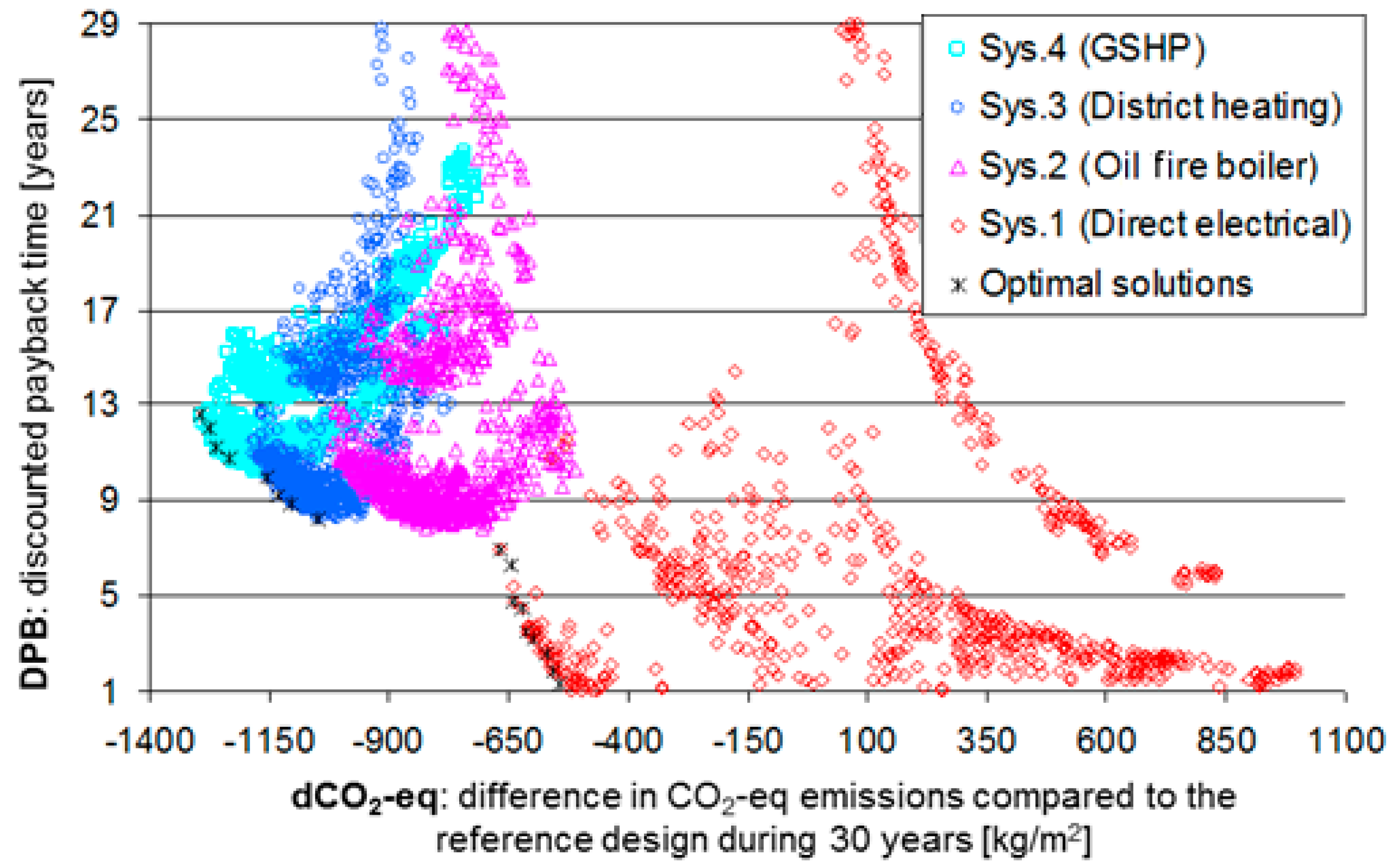
Case 1 assumes 4% real interest rate and 2%, 3.5%, and 3% energy price escalation rates for electricity, light fuel, and district heating, respectively. Case 2 assumes different rates, 1% real interest rate and 4%, 7%, and 6% energy price escalation rates. The latter rates better represent the economic situation in Finland during the last decade. Figure 7 presents the results for Case 2, showing that the payback times of Case 2 are shorter than those of Case 1.
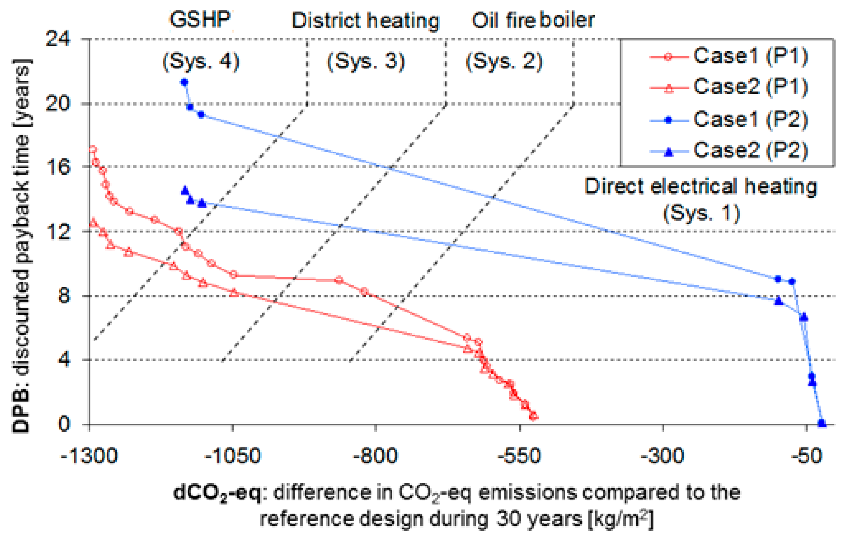
Indeed, the lower real interest rate and the higher energy-price escalation rates promote the economic viability of the investments that are spent to reduce the CO2-eq emissions. It is also worthwhile to mention that, based on the economic assumptions of Case 2, the oil fire heating system could not compete with the other heating systems. The discussed optimal solutions (Pareto fronts) of Case 1 and 2 neglect the increase in summertime overheating that can occur due to the presence of additional thermal insulation and/or tighter building envelope. Figure 8 shows the two discussed Pareto fronts, denoted as (P1) and Case 2 (P1), respectively. In the same figure, two other Pareto fronts, i.e., Case 1 (P2) and Case 2 (P2), are presented. These latter consider the summertime overheating of the reference design (DH24 = 2400 °C.h) as a constraint, i.e., an upper limit that cannot be exceed. All Pareto solutions for the four case studies are characterized in Appendix A.
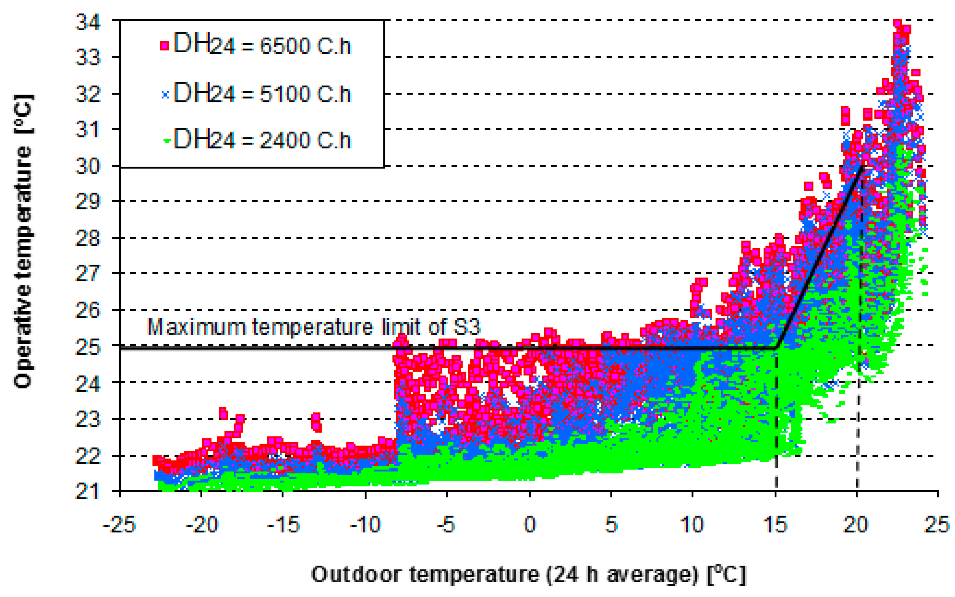
The summer overheating is assessed by the degree hours (DH24) as defined in Section 2.1.3. Higher DH24 means more summertime overheating. The optimal solutions of Case 1(P1) and Case 2(P1) have high levels of DH24 (from 5100 to 6200 °C.h vs. 2400 °C.h for the reference case). The reason is that energy saving measures (e.g., additional insulation, no shading, or tighter building envelope) are selected as low-emission cost-effective solutions, but they can exert a negative effect in summertime, i.e., the overheating effect. Indeed, if the upper limits of insulation, solar heat gain, and building tightness are used as a building envelope combination, the DH24 reaches 6500 °C.h. However for economic considerations, this combination is not selected as an optimal solution. Finally, Figure 9 presents the indoor operative air temperature for different levels of summer overheating (DH24 = 2400, 5100, and 6500 °C.h). The maximum and minimum temperature limits of S3-2008 Finnish indoor climate classification are also presented in the same figure. S3 Class is in line with the official indoor air quality set by building codes. The S3 Class defines the maximum acceptable overheating levels for buildings without mechanical cooling.
The results show that the thermal comfort level of the reference design meets the S3-2008 Finnish indoor climate classification (i.e., the operative air temperature at the warmest zone is lower than the maximum acceptable limit). However, the lowest summer overheating level (DH24 = 5100 °C.h) of Case 1 (P1) and Case 2 (P1) optimal solutions exceed the maximum temperature limit. In order to make those solutions be acceptable, additional natural ventilation measures (e.g., larger area of operable windows) should be implemented.
Case 1(P2) and Case 2(P2) consider DH24 = 2400 °C.h as a constraint. This limits the implementation of additional insulation, lower U-value window type, and/or tighter building envelope. Clearly, reducing the domain of the energy saving options increases the payback time of the available low-emission measures (better efficiency heat recovery unit and lower emission heating system). Using less energy saving measures, the oil fire heating and the district heating system could not compete with the GSHP as low-emission cost-effective optimal solutions. Notably, based on the applied constraint, the shortest payback time of the oil fire and the district heating optimal solutions is 24 years, which is longer than 22 years, i.e., the longest payback time of the GSHP optimal solutions. Thus, finally, the GSHP is the most cost-effective and low-carbon solution, which, at the same time, does not cause summer overheating. Definitely, it provides the best trade-off between collective and private perspectives. Compared to [12], the outcomes better address the mentioned perspectives because they provide more meaningful economic and environmental indicators. Indeed, diversely from [12], CO2-eq emissions take account of emissions due to embodied energies of insulation volume and windows too, thereby ensuring a more accurate evaluation of environmental burdens for the collective perspective. In addition, in [12] the second objective function was the minimization of investment cost, whereas the current study considers the minimization of payback time, which definitely provides a more appropriate assessment of investments’ cost-effectiveness for the private perspective. Most notably, this objective function allows to identify energy saving measures that are really profitable, as shown by the achieved outcomes. Indeed, these latter clearly show that the most low-carbon and cost-effective solution is the GSHP in all investigated case studies, whereas in [12] the cost-effectiveness of this system is underestimated because of the high initial investment costs.
5. Sensitivity of the Results: Discussion
The main goal of the paper was to provide a robust optimization methodology to address and guide building energy design by pursuing the best trade-off between collective and private interests. Clearly, the final choice requires multi-criteria decision-making, which is affected by the importance that is given to each objective function, and thus to each perspective. Therefore, it depends on involved stakeholders’ needs and wills, as well as on the weight of each stakeholder in the decision process. The proposed methodology supports this process by reducing the domain of possible choices, since it provides a limited number of optimal trade-off solutions. In other words, it simplifies the decision-making, which represents one of the main issues of human race. The application to the investigated case study shows such great potential. In this regard, the examined building can be considered representative of a good share of Finnish dwellings, as concerns thermal characteristics of building envelope and type of HVAC systems. Therefore, the achieved conclusions can be extended to several similar case studies, especially as regards the significant environmental and economic benefits that can be produced by the installation of GSHPs. This is particularly worthwhile because, as aforementioned, single-family houses are one of the main CO2-eq emission source in the countries of EU. Thus, the wide diffusion of GSHPs in Finland would imply a substantial reduction of greenhouse polluting emissions ensuring, at the same time, large economic benefits for the private. Definitely, the achieved outcomes are sensible to different factors, such as:
- environmental assumptions, as concerns the values of the emission factors, which are assumed fixed as justified in Section 3.1;
- economic assumptions, e.g., discount rate and energy prices, which are subjected to high volatility; this variability is taken into account by considering the two economic scenarios characterized in Table 1. Definitely, the optimal solutions are sensitive to the economic assumptions, but globally the GSHP is the best trade-off solution between collective and private perspectives;
- macro-climatic scenario, which can be affected by global warming (the worst forecasts provide an increase of average outdoor temperature of around 1.8 °C by 2050). Surely, global warming can affect building energy performance in terms of reduction of heating demand and increase of summer overheating risk. However, these effects are significant in the long period, while the influence of global warming is quite low in smaller periods (around 10–20 years), such as the payback times of the optimal energy design solutions (see Figure 8). Therefore, global warming is here neglected and a reliable average weather data file is employed. Furthermore, different scenarios should be explored to achieve a robust assessment of global warming effects, requiring substantial computational times (the optimization procedure should be implemented for each scenario). Thus, this investigation requires a dedicated analysis, which will be conducted in future studies;
- micro-climatic scenario, which depends on micro-climatic phenomena, e.g., heat island effect, and urban context, e.g., isolated or adjacent buildings. The developed methodology can take account of this variability, for instance by properly modifying the weather data file or considering the inter-building effect. However, also in this case a dedicated analysis is required because of the amount of needed computational burden;
- occupant behavior, which, in most cases, represents the most influential factor on building energy performance; however, it is characterized by high levels of uncertainty and volatility, and thus it is often unpredictable. Thus, as for the previous factors, different scenarios should be explored for a robust assessment, and this requires a dedicated analysis, which is not included among the objectives of this study.
As shown, building energy performance is affected by a large number of factors and considering all possible scenarios is prohibitive from a computational point of view when robust but time-consuming optimization methodologies are used. In addition, this study is focused on the presentation of the optimization approach for addressing building energy design, and future works will examine the sensitivity of the optimal solutions to some of the listed factors. Only the sensitivity to the macro-economic scenario is here taken into account because this can exert a substantial influence on the cost-effectiveness of energy conservation measures [29]. On the other hand, considering the sensitivity to all described factors would be prohibitive, as aforementioned, and furthermore it would imply high complexity in the interpretation of the outcomes for the stakeholders. Indeed, a huge number of sets of optimal solutions would be achieved (i.e., one set for each combination among the examined scenarios) thereby complicating the decision-making, whereas supporting the decision is the aim of the proposed methodology. In this regard, providing one or few sets of optimal solutions concerning one of few average scenarios is better than providing a huge amount of outcomes that consider the variability of the descried factors but are difficult to be interpreted.
Finally, it is noted that the methodology can be applied to different case studies as concerns building typology, use destination, climatic location, since IDA ICE enables a comprehensive energy modeling and simulation of any building type. Moreover, as delineated in Section 2.2.1, the optimization scheme allows to consider a wide set of energy conservation measures, concerning building envelope, operation, energy systems and exploitation of renewable energy sources. Thus, the proposed methodology can be employed to optimize the energy design of any new or existing building by pursuing the trade-off between collective and private perspectives. Definitely, it is not user-friendly because it requires high expertise in building energy modeling (through IDA ICE), programming (through MATLAB®) and optimization techniques. Future studies will address this issue in order to develop a powerful tool that can be used by a significant share of professionals in matter of building energy performance.
6. Conclusions
The finical viability and the environmental impact of 13,456 integrated building solutions are assessed for a single-family dwelling in the cold climate of Helsinki, Finland. The building solutions concern energy design and include different options for eight design variables: insulation thickness of external walls, floor and roof, type of window glazing, window shading, heat recovery, level of building tightness and heating systems.
The Pareto front concept is applied and a bi-objective optimization is implemented by running a modified GA in order to identify low-emission cost-effective design solutions. In particular, CO2-eq emissions and discounted payback period are minimized in order to reconcile the main actors involved in the optimization of building energy performance, namely the collectivity and the private sector. The results show that lower real interest rate and higher energy price escalation rates promote, clearly, the economic viability of low-energy low-emission measures. Notably, the type of heating energy source has a marked influence on the results. The payback time of the GSHP (ground source heat pump) optimal integrated solutions ranges from 10–22 years. This heating system can imply the highest reduction in CO2-eq emissions, around 1300 kgCO2-eq/m2, with 17 year DPB; the oil fire boiler can imply the lowest DPB, equal to 8.5 years, with 850 kgCO2-eq/m2 reduction. In addition, it is shown that lower summer-overheating solutions accept less energy saving options. This leads to longer payback times. Furthermore, the Finnish statistics state that the energy-price escalation rate of light oil and district heating is higher than the one of electricity. Hence, the oil fire boiler and the district heating need to be integrated with additional energy saving measures in order to produce significant reductions of polluting emissions and reasonable payback times thereby competing with electrical supply heating systems.
In this framework, about 60% of the Finnish detached and row house stock uses electrical heating. Thus, establishing new nuclear or renewable power stations (e.g., biofuel combined heat and power or centralized photovoltaic stations) would reduce the specific electricity price, thereby mitigating the environmental burdens of the existing building stock and enhancing the profitability of GSHPs as low-emission heating systems for new buildings.
Author Contributions
The research was carried out by both authors through a synergic collaboration and continuous reciprocal feedbacks. The authors contributed in all phases of the work.
Conflicts of Interest
The authors declare no conflict of interest.
Appendix A

Table A1.
Optimal Pareto solutions for Case 1 (P1).
| dCO2 | DPB | DH24 | dE | dIC | Ubldg | X1 | X2 | X3 | X4 | X5 | X6 | X7 | X8 |
|---|---|---|---|---|---|---|---|---|---|---|---|---|---|
| −525.8 | 0.4 | 5755.9 | −46.9 | 1.1 | 0.20 | 0.25 | 0.36 | 0.18 | 3 | 3 | 2 | 3 | 1 |
| −540.0 | 1.3 | 5764.7 | −47.7 | 5.9 | 0.18 | 0.32 | 0.19 | 0.19 | 4 | 2 | 2 | 3 | 1 |
| −558.2 | 1.9 | 5841.9 | −50.0 | 8.4 | 0.18 | 0.30 | 0.32 | 0.27 | 3 | 3 | 2 | 3 | 1 |
| −564.9 | 2.4 | 5912.1 | −51.6 | 11.2 | 0.17 | 0.32 | 0.36 | 0.29 | 3 | 3 | 2 | 3 | 1 |
| −583.2 | 2.8 | 5945.4 | −51.6 | 13.0 | 0.17 | 0.27 | 0.36 | 0.29 | 4 | 3 | 2 | 3 | 1 |
| −606.5 | 3.6 | 5952.8 | −53.3 | 17.9 | 0.18 | 0.27 | 0.36 | 0.29 | 3 | 3 | 2 | 4 | 1 |
| −611.6 | 3.9 | 6080.7 | −53.7 | 20.6 | 0.17 | 0.27 | 0.37 | 0.28 | 4 | 2 | 2 | 4 | 1 |
| −620.2 | 5.1 | 6166.1 | −57.4 | 27.4 | 0.15 | 0.35 | 0.45 | 0.36 | 3 | 3 | 2 | 4 | 1 |
| −641.4 | 5.3 | 6219.2 | −57.5 | 28.6 | 0.15 | 0.30 | 0.45 | 0.34 | 4 | 3 | 2 | 4 | 1 |
| −819.6 | 8.3 | 5111.4 | −26.8 | 39.7 | 0.25 | 0.21 | 0.15 | 0.11 | 2 | 2 | 2 | 1 | 2 |
| −862.3 | 8.9 | 5358.7 | −33.2 | 46.7 | 0.22 | 0.23 | 0.21 | 0.17 | 3 | 2 | 2 | 1 | 2 |
| −1047.1 | 9.3 | 5111.4 | −26.8 | 46.7 | 0.25 | 0.21 | 0.15 | 0.11 | 2 | 2 | 2 | 1 | 3 |
| −1087.7 | 10.0 | 5116.0 | −28.4 | 51.6 | 0.28 | 0.21 | 0.27 | 0.09 | 1 | 2 | 2 | 2 | 3 |
| −1108.9 | 10.6 | 5464.2 | −37.9 | 60.4 | 0.21 | 0.22 | 0.21 | 0.21 | 3 | 2 | 2 | 2 | 3 |
| −1129.9 | 11.0 | 5306.7 | −35.9 | 61.5 | 0.25 | 0.24 | 0.27 | 0.12 | 1 | 2 | 2 | 3 | 3 |
| −1143.6 | 12.0 | 5635.3 | −44.2 | 73.0 | 0.19 | 0.26 | 0.18 | 0.29 | 3 | 2 | 2 | 3 | 3 |
| −1184.3 | 12.7 | 5159.2 | −27.6 | 74.3 | 0.25 | 0.21 | 0.19 | 0.11 | 2 | 2 | 2 | 1 | 4 |
| −1228.5 | 13.3 | 5191.3 | −31.8 | 80.3 | 0.26 | 0.28 | 0.20 | 0.11 | 1 | 2 | 2 | 2 | 4 |
| −1254.8 | 13.8 | 5306.7 | −35.9 | 86.5 | 0.25 | 0.24 | 0.27 | 0.12 | 1 | 2 | 2 | 3 | 4 |
| −1262.9 | 14.2 | 5156.1 | −32.0 | 85.6 | 0.27 | 0.18 | 0.22 | 0.14 | 1 | 3 | 2 | 3 | 4 |
| −1269.6 | 14.9 | 5378.4 | −39.6 | 96.3 | 0.22 | 0.28 | 0.19 | 0.24 | 1 | 2 | 2 | 3 | 4 |
| −1274.4 | 15.8 | 5643.5 | −46.9 | 105.9 | 0.20 | 0.20 | 0.30 | 0.31 | 2 | 3 | 2 | 4 | 4 |
| −1287.2 | 16.3 | 5789.6 | −50.4 | 111.9 | 0.19 | 0.25 | 0.24 | 0.32 | 3 | 3 | 2 | 4 | 4 |
| −1291.9 | 17.1 | 5766.0 | −47.8 | 116.2 | 0.19 | 0.19 | 0.25 | 0.42 | 4 | 2 | 2 | 4 | 4 |
dCO2: difference in CO2-eq emissions during 30 years; DPB: discounted payback time of the additional investments compared with the reference design (years); DH24: degree hours (number of hours at which the operative temperature >24 °C); dE: difference in the annual heating energy consumption (kWh/m2); dIC: difference in investment cost (€/m2); Ubldg: overall building envelope thermal transmittance (W/m2 K); X1: thickness of the external wall insulation (m) (Table 3); X2: thickness of the roof insulation (m) (Table 3); X3: thickness of the floor insulation (m) (Table 3); X4: window type (Table 4); X5: heat recovery type (Table 5); X6: shading option (Table 6); X7: building tightness (Table 7); X8: heating system type (Table 8).
Table A2.
Optimal Pareto solutions for Case 2 (P1).
| dCO2 | DPB | DH24 | dE | dIC | Ubldg | X1 | X2 | X3 | X4 | X5 | X6 | X7 | X8 |
|---|---|---|---|---|---|---|---|---|---|---|---|---|---|
| −525.8 | 0.6 | 5755.9 | −46.9 | 1.1 | 0.20 | 0.25 | 0.36 | 0.18 | 3 | 3 | 2 | 3 | 1 |
| −540.0 | 1.3 | 5764.7 | −47.7 | 5.9 | 0.18 | 0.32 | 0.19 | 0.19 | 4 | 2 | 2 | 3 | 1 |
| −558.2 | 1.8 | 5841.9 | −50.0 | 8.4 | 0.18 | 0.30 | 0.32 | 0.27 | 3 | 3 | 2 | 3 | 1 |
| −570.3 | 2.6 | 5717.3 | −48.4 | 13.4 | 0.19 | 0.26 | 0.18 | 0.30 | 3 | 2 | 2 | 4 | 1 |
| −595.7 | 3.2 | 5789.6 | −50.4 | 15.9 | 0.19 | 0.25 | 0.24 | 0.32 | 3 | 3 | 2 | 4 | 1 |
| −611.6 | 3.5 | 6080.7 | −53.7 | 20.6 | 0.17 | 0.27 | 0.37 | 0.28 | 4 | 2 | 2 | 4 | 1 |
| −620.2 | 4.5 | 6166.1 | −57.4 | 27.4 | 0.15 | 0.35 | 0.45 | 0.36 | 3 | 3 | 2 | 4 | 1 |
| −641.4 | 4.8 | 6219.2 | −57.5 | 28.6 | 0.15 | 0.30 | 0.45 | 0.34 | 4 | 3 | 2 | 4 | 1 |
| −1047.1 | 8.3 | 5111.4 | −26.8 | 46.7 | 0.25 | 0.21 | 0.15 | 0.11 | 2 | 2 | 2 | 1 | 3 |
| −1102.4 | 8.8 | 5428.9 | −36.3 | 58.1 | 0.22 | 0.21 | 0.22 | 0.18 | 3 | 2 | 2 | 2 | 3 |
| −1129.9 | 9.3 | 5306.7 | −35.9 | 61.5 | 0.25 | 0.24 | 0.27 | 0.12 | 1 | 2 | 2 | 3 | 3 |
| −1151.9 | 9.9 | 5654.8 | −44.2 | 73.6 | 0.19 | 0.24 | 0.18 | 0.23 | 4 | 2 | 2 | 3 | 3 |
| −1231.3 | 10.8 | 5464.2 | −37.9 | 85.4 | 0.21 | 0.22 | 0.21 | 0.21 | 3 | 2 | 2 | 2 | 4 |
| −1262.9 | 11.3 | 5156.1 | −32.0 | 85.6 | 0.27 | 0.18 | 0.22 | 0.14 | 1 | 3 | 2 | 3 | 4 |
| −1274.4 | 12.0 | 5643.5 | −46.9 | 105.9 | 0.20 | 0.20 | 0.30 | 0.31 | 2 | 3 | 2 | 4 | 4 |
| −1291.9 | 12.6 | 5766.0 | −47.8 | 116.2 | 0.19 | 0.19 | 0.25 | 0.42 | 4 | 2 | 2 | 4 | 4 |
dCO2: difference in CO2-eq emissions during 30 years; DPB: discounted payback time of the additional investments compared with the reference design (years); DH24: degree hours (number of hours at which the operative temperature >24 °C); dE: difference in the annual heating energy consumption (kWh/m2); dIC: difference in investment cost (€/m2); Ubldg: overall building envelope thermal transmittance (W/m2 K); X1: thickness of the external wall insulation (m) (Table 3); X2: thickness of the roof insulation (m) (Table 3); X3: thickness of the floor insulation (m) (Table 3); X4: window type (Table 4); X5: heat recovery type (Table 5); X6: shading option (Table 6); X7: building tightness (Table 7); X8: heating system type (Table 8).
Table A3.
Optimal Pareto solutions for Case 1 (P2).
| dCO2 | DPB | DH24 | dE | dIC | Ubldg | X1 | X2 | X3 | X4 | X5 | X6 | X7 | X8 |
|---|---|---|---|---|---|---|---|---|---|---|---|---|---|
| −39.0 | 3.0 | 2390.6 | −2.9 | 0.9 | 0.30 | 0.11 | 0.24 | 0.15 | 1 | 2 | 1 | 1 | 1 |
| −72.7 | 8.8 | 2388.5 | −8.4 | 6.0 | 0.36 | 0.29 | 0.11 | 0.04 | 1 | 3 | 1 | 1 | 1 |
| −99.3 | 9.0 | 2398.3 | −10.9 | 8.2 | 0.35 | 0.29 | 0.16 | 0.04 | 1 | 3 | 1 | 1 | 1 |
| −1123.0 | 19.7 | 2390.6 | −2.9 | 96.9 | 0.30 | 0.11 | 0.24 | 0.15 | 1 | 2 | 1 | 1 | 4 |
| −1132.1 | 21.3 | 2398.3 | 0.2 | 101.6 | 0.33 | 0.10 | 0.11 | 0.21 | 1 | 2 | 1 | 2 | 4 |
Table A4.
Optimal Pareto solutions for Case 2 (P2).
| dCO2 | DPB | DH24 | dE | dIC | Ubldg | X1 | X2 | X3 | X4 | X5 | X6 | X7 | X8 |
|---|---|---|---|---|---|---|---|---|---|---|---|---|---|
| −39.0 | 2.8 | 2390.6 | −2.9 | 0.9 | 0.30 | 0.11 | 0.24 | 0.15 | 1 | 2 | 1 | 1 | 1 |
| −52.9 | 6.8 | 2378.2 | −7.0 | 5.5 | 0.36 | 0.29 | 0.11 | 0.04 | 1 | 2 | 1 | 1 | 1 |
| −99.3 | 7.7 | 2398.3 | −10.9 | 8.2 | 0.35 | 0.29 | 0.16 | 0.04 | 1 | 3 | 1 | 1 | 1 |
| −1123.0 | 14.0 | 2390.6 | −2.9 | 96.9 | 0.30 | 0.11 | 0.24 | 0.15 | 1 | 2 | 1 | 1 | 4 |
| −1132.1 | 14.7 | 2398.3 | 0.2 | 101.6 | 0.33 | 0.10 | 0.11 | 0.21 | 1 | 2 | 1 | 2 | 4 |
dCO2: difference in CO2-eq emissions during 30 years; DPB: discounted payback time of the additional investments compared with the reference design (years); DH24: degree hours (number of hours at which the operative temperature >24 °C); dE: difference in the annual heating energy consumption (kWh/m2); dIC: difference in investment cost (€/m2); Ubldg: overall building envelope thermal transmittance (W/m2 K); X1: thickness of the external wall insulation (m) (Table 3); X2: thickness of the roof insulation (m) (Table 3); X3: thickness of the floor insulation (m) (Table 3); X4: window type (Table 4); X5: heat recovery type (Table 5); X6: shading option (Table 6); X7: building tightness (Table 7); X8: heating system type (Table 8).
References
- International Energy Agency (IEA). IEA: Paris, France. Available online: https://www.iea.org/statistics/ (accessed on 8 March 2017).
- Khatib, H. IEA world energy outlook 2011—A comment. Energy Policy 2012, 48, 737–743. [Google Scholar] [CrossRef]
- Santamouris, M. Innovating to zero the building sector in Europe: Minimising the energy consumption, eradication of the energy poverty and mitigating the local climate change. Sol. Energy 2016, 128, 61–94. [Google Scholar] [CrossRef]
- US Department of Energy. Energy Efficiency and Renewable Energy Office, Building Technology Program (2013), EnergyPlus 8.0.0. Available online: https://energyplus.net/downloads (accessed on 9 March 2017).
- Solar Energy Laboratory; Klein, S.A. TRNSYS: A Transient System Simulation Program; University of Wisconsin: Madison, WI, USA, 1979. [Google Scholar]
- ESP-r. Available online: http://www.esru.strath.ac.uk/Programs/ESP-r.htm (accessed on 9 March 2017).
- IDA ICE. IDA Indoor Climate and Energy. Available online: http://www.equa.se/en/ida-ice (accessed on 9 March 2017).
- Nguyen, A.T.; Reiter, S.; Rigo, P. A review on simulation-based optimization methods applied to building performance analysis. Appl. Energy 2014, 113, 1043–1058. [Google Scholar] [CrossRef]
- Ascione, F.; Bianco, N.; De Stasio, C.; Mauro, G.M.; Vanoli, G.P. A new comprehensive approach for cost-optimal building design integrated with the multi-objective model predictive control of HVAC systems. Sustain. Cities Soc. 2017, 31, 136–150. [Google Scholar] [CrossRef]
- Ascione, F.; Bianco, N.; De Masi, R.F.; De Stasio, C.; Mauro, G.M.; Vanoli, G.P. Multi-objective optimization of the renewable energy mix for a building. Appl. Ther. Eng. 2016, 101, 612–621. [Google Scholar] [CrossRef]
- Ascione, F.; Bianco, N.; De Stasio, C.; Mauro, G.M.; Vanoli, G.P. A new methodology for cost-optimal analysis by means of the multi-objective optimization of building energy performance. Energy Build. 2015, 88, 78–90. [Google Scholar] [CrossRef]
- Hamdy, M.; Hasan, A.; Siren, K. Applying a multi-objective optimization approach for design of low-emission cost-effective dwellings. Build. Environ. 2011, 46, 109–123. [Google Scholar] [CrossRef]
- Hamdy, M.; Hasan, A.; Siren, K. A multi-stage optimization method for cost-optimal and nearly-zero-energy building solutions in line with the EPBD-recast 2010. Energy Build. 2013, 56, 189–203. [Google Scholar] [CrossRef]
- Attia, S.; Hamdy, M.; O’Brien, W.; Carlucci, S. Assessing gaps and needs for integrating building performance optimization tools in net zero energy buildings design. Energy Build. 2013, 60, 110–124. [Google Scholar] [CrossRef]
- Machairas, V.; Tsangrassoulis, A.; Axarli, K. Algorithms for optimization of building design: A review. Renew. Sustain. Energy Rev. 2014, 31, 101–112. [Google Scholar] [CrossRef]
- Hamdy, M.; Nguyen, A.T.; Hensen, J.L. A performance comparison of multi-objective optimization algorithms for solving nearly-zero-energy-building design problems. Energy Build. 2016, 121, 57–71. [Google Scholar] [CrossRef]
- Li, K.; Pan, L.; Xue, W.; Jiang, H.; Mao, H. Multi-Objective Optimization for Energy Performance Improvement of Residential Buildings: A Comparative Study. Energies 2017, 10, 245. [Google Scholar] [CrossRef]
- MATLAB®, MATrixLABoratory—7.10.0, User’s Guide; MathWorks: Natick, MA, USA, 2010.
- Delgarm, N.; Sajadi, B.; Delgarm, S. Multi-objective optimization of building energy performance and indoor thermal comfort: A new method using artificial bee colony (ABC). Energy Build. 2016, 131, 42–53. [Google Scholar] [CrossRef]
- Yang, M.D.; Lin, M.D.; Lin, Y.H.; Tsai, K.T. Multiobjective optimization design of green building envelope material using a non-dominated sorting genetic algorithm. Appl. Ther. Eng. 2017, 111, 1255–1264. [Google Scholar] [CrossRef]
- Bre, F.; Silva, A.S.; Ghisi, E.; Fachinotti, V.D. Residential building design optimisation using sensitivity analysis and genetic algorithm. Energy Build. 2016, 133, 853–866. [Google Scholar] [CrossRef]
- Brunelli, C.; Castellani, F.; Garinei, A.; Biondi, L.; Marconi, M. A Procedure to Perform Multi-Objective Optimization for Sustainable Design of Buildings. Energies 2016, 9, 915. [Google Scholar] [CrossRef]
- Fan, Y.; Xia, X. A multi-objective optimization model for energy-efficiency building envelope retrofitting plan with rooftop PV system installation and maintenance. Appl. Energy 2017, 189, 327–335. [Google Scholar] [CrossRef]
- Salata, F.; Golasi, I.; Domestico, U.; Banditelli, M.; Basso, G.L.; Nastasi, B.; de Lieto Vollaro, A. Heading towards the nZEB through CHP+ HP systems. A comparison between retrofit solutions able to increase the energy performance for the heating and domestic hot water production in residential buildings. Energy Convers. Manag. 2017, 138, 61–76. [Google Scholar] [CrossRef]
- Kerdan, I.G.; Raslan, R.; Ruyssevelt, P.; Gálvez, D.M. ExRET-Opt: An automated exergy/exergoeconomic simulation framework for building energy retrofit analysis and design optimisation. Appl. Energy 2017, 192, 33–58. [Google Scholar] [CrossRef]
- Wu, R.; Mavromatidis, G.; Orehounig, K.; Carmeliet, J. Multiobjective optimisation of energy systems and building envelope retrofit in a residential community. Appl. Energy 2017, 190, 634–649. [Google Scholar] [CrossRef]
- Ascione, F.; Bianco, N.; De Stasio, C.; Mauro, G.M.; Vanoli, G.P. Multi-stage and multi-objective optimization for energy retrofitting a developed hospital reference building: A new approach to assess cost-optimality. Appl. Energy 2016, 174, 37–68. [Google Scholar] [CrossRef]
- Ascione, F.; Bianco, N.; De Stasio, C.; Mauro, G.M.; Vanoli, G.P. CASA, cost-optimal analysis by multi-objective optimisation and artificial neural networks: A new framework for the robust assessment of cost-optimal energy retrofit, feasible for any building. Energy Build. 2017, 146, 200–219. [Google Scholar] [CrossRef]
- Ascione, F.; Bianco, N.; De Masi, R.F.; Mauro, G.M.; Vanoli, G.P. Energy retrofit of educational buildings: Transient energy simulations, model calibration and multi-objective optimization towards nearly zero-energy performance. Energy Build. 2017, 144, 303–319. [Google Scholar] [CrossRef]
- Mauro, G.M.; Menna, C.; Vitiello, U.; Asprone, D.; Ascione, F.; Bianco, N.; Prota, A.; Vanoli, G.P. A Multi-Step Approach to Assess the Lifecycle Economic Impact of Seismic Risk on Optimal Energy Retrofit. Sustainability 2017, 9, 989. [Google Scholar] [CrossRef]
- Mostavi, E.; Asadi, S.; Boussaa, D. Development of a new methodology to optimize building life cycle cost, environmental impacts, and occupant satisfaction. Energy 2017, 121, 606–615. [Google Scholar] [CrossRef]
- Delgarm, N.; Sajadi, B.; Delgarm, S.; Kowsary, F. A novel approach for the simulation-based optimization of the buildings energy consumption using NSGA-II: Case study in Iran. Energy Build. 2016, 127, 552–560. [Google Scholar] [CrossRef]
- Harmathy, N.; Magyar, Z.; Folić, R. Multi-criterion optimization of building envelope in the function of indoor illumination quality towards overall energy performance improvement. Energy 2016, 114, 302–317. [Google Scholar] [CrossRef]
- Holopainen, R.; Hekkanen, M. Energy renovation saving potentials of typical Finnish buildings. In Proceedings of the 8th Symposium on Building Physics in the Nordic Countries, Copenhagen, Denmark, 16–18 June 2008. [Google Scholar]
- Kara, M.; Syri, S.; Lehtilä, A.; Helynen, S.; Kekkonen, V.; Ruska, M.; Forsström, J. The impacts of EU CO2 emissions trading on electricity markets and electricity consumers in Finland. Energy Econ. 2008, 30, 193–211. [Google Scholar] [CrossRef]
- Pylsy, P.; Kalema, T. Research Report 1: Concepts for Low-Energy Single-Family Houses; Tampere University of Technology: Tampere, Finland, 2008. [Google Scholar]
- Hasan, A.; Vuolle, M.; Sirén, K. Minimisation of life cycle cost of a detached house using combined simulation and optimisation. Build. Environ. 2008, 43, 2022–2034. [Google Scholar] [CrossRef]
- Alanne, K.; Salo, A.; Saari, A.; Gustafsson, S.I. Multi-criteria evaluation of residential energy supply systems. Energy Build. 2007, 39, 1218–1226. [Google Scholar] [CrossRef]
- Hamdy, M.; Hasan, A.; Siren, K. Optimum design of a house and its HVAC systems using simulation-based optimisation. Int. J. Low-Carbon Technol. 2010, 5, 120–124. [Google Scholar] [CrossRef]
- Petersdorff, C.; Boermans, T.; Harnisch, J. Mitigation of CO2 emissions from the EU-15 building stock. beyond the EU directive on the energy performance of buildings. Environ. Sci. Pollut. Res. 2006, 13, 350–358. [Google Scholar] [CrossRef]
- Travesi, J.; Maxwell, G.; Klaassen, C.; Holtz, M.; Knabe, G.; Felsmann, C.; Behne, M. Empirical validation of Iowa energy resource station building energy analysis simulation models. IEA Task 2001, 22. [Google Scholar]
- Achermann, M.; Zweifel, G. RADTEST–Radiant Heating and Cooling Test Cases. A Report of Task 22, Subtask C; International Energy Agency (IEA): Luzern, Switzerland, 2003. [Google Scholar]
- Woloszyn, M.; Rode, C. Tools for performance simulation of heat, air and moisture conditions of whole buildings. Build. Simul. 2008, 1, 5–24. [Google Scholar] [CrossRef]
- EU Commission and Parliament, Directive 2010/31/EU of the European Parliament and of the Council of 19 May 2010 on the Energy Performance of Buildings (EPBD Recast). Available online: http://eur-lex.europa.eu/legal-content/EN/TXT/?uri=CELEX%3A32010L0031 (accessed on 15 July 2017).
- EU Commission, Commission Delegated Regulation (EU) No 244/2012 of 16 January 2012 Supplementing Directive 2010/31/EU of the European Parliament and of the Council on the Energy Performance of Buildings. Available online: http://www.eib.org/epec/ee/documents/comparative-methodology-epbd.pdf (accessed on 15 July 2017).
- Heljo, J.; Laine, H. Institute of Construction Economics, Report 2; Tampere University of Technology: Tampere, Finland, 2005. [Google Scholar]
- Hammond, G.; Jones, C. Inventory of Carbon and Energy (ICE), version 1.6a; University of Bath: Bath, UK, 2008. [Google Scholar]
- Asif, M.; Davidson, A.; Muneer, T. Embodied energy analysis of aluminium-clad windows. Build. Ser. Eng. Res. Technol. 2001, 22, 195–199. [Google Scholar] [CrossRef]
- Jaluria, Y. Design and Optimization of Thermal Systems; CRC Press: Boca Raton, FL, USA, 2007. [Google Scholar]
- Fuller, S.; Petersen, S. Life-Cycle Costing Manual for the Federal Energy Management Program, 1995 Edition. In NIST Handbook; NIST: Gaithersburg, MD, USA, 1996; p. 135. [Google Scholar]
- Deb, K. Multi-Objective Optimization Using Evolutionary Algorithms; John Wiley & Sons: Chichester, UK, 2001. [Google Scholar]
- Hamdy, M. Combining Simulation and Optimisation for Dimensioning Optimal Building Envelopes and HVAC Systems. Ph.D. Thesis, Aalto University, Aalto, Finland, 2012. [Google Scholar]
- Kalamees, T.; Jylhä, K.; Tietäväinen, H.; Jokisalo, J.; Ilomets, S.; Hyvönen, R.; Saku, S. Development of weighting factors for climate variables for selecting the energy reference year according to the EN ISO 15927-4 standard. Energy Build. 2012, 47, 53–60. [Google Scholar] [CrossRef]
- The National Building Code of Finland D5. Calculation of Power and Energy Needs for Heating of Buildings, Guidelines; Ministry of the Environment: Helsinki, Finland, 2007; p. 72.
- D2 Finland Code of Building Regulation. Indoor Climate and Ventilation of Buildings, Regulation and Guidelines; Ministry of Environment: Helsinki, Finland, 2003.
- Energy Statistics Finland (Calculated with Benefit Allocation Method). Available online: http://www.stat.fi/index_en.html (accessed on 25 February 2011).
- Manczyk, H. Life Cycle Cost Analysis: Selection of Heating Equipment, Manczyk Energy Consulting. 2003.
- Collins, T.; Parker, S.A.; Baxter, V. Assessment of Hybrid Geothermal Heat Pump Systems, Technology Installation Review; U.S. Department of Energy: Washington, DC, USA, 2001.
- Saari, A.; Kalamees, T.; Jokisalo, J.; Michelsson, R.; Alanne, K.; Kurnitski, J. Financial viability of energy-efficiency measures in a new detached house design in Finland. Appl. Energy 2012, 92, 76–83. [Google Scholar] [CrossRef]
- Consumer Price Index, Statistics Finland. Available online: http://www.stat.fi/index_en.html (accessed on 25 February 2011).
- Reuters (Bank of Finland). Available online: www.bof.fi/Stats/default.aspx?r=%2ftilastot%2fmarkkina_ja_hallinnolliset_korot%2feuriborkorot_kk_chrt_en (accessed on 25 February 2011).
- Finnish Statistic Office. Available online: www.stat.fi/til/ehkh/tau_en.html (accessed on 25 February 2011).
- The National Building Code of Finland C3. Thermal Insulation in a Building, Regulations; Ministry of the Environment: Helsinki, Finland, 2007; p. 9.
- Sahlin, P. Modelling and Simulation Methods for Modular Continuous System in Buildings. Ph.D. Thesis, KTH, Stockholm, Sweden, 1996. [Google Scholar]
- Aalto University School of Engineering. Environmental Aspects of Building Construction with Green Materials Case Lahti. Available online: www.adv-trade.ru/files/fenestra_windowbrochure.pdf (accessed on 25 February 2011).
- Björsell, N.; Bring, A.; Eriksson, L.; Grozman, P.; Lindgren, M.; Sahlin, P.; Vuolle, M. IDA indoor climate and energy. In Proceedings of the 6-th IBPSA Conference, Kyoto, Japan, 13–15 September 1999; pp. 1035–1042. [Google Scholar]
- Tamar on Enemmän. Available online: www.tamar.fi (accessed on 25 February 2011).
Figure 1.
Optimization scheme: coupling between MATLAB® and IDA ICE.

Figure 2.
The investigated two-storey dwelling.

Figure 3.
The specific emissions of the district heating energy [56].
Figure 3.
The specific emissions of the district heating energy [56].

Figure 4.
Year-on-year changes in the Consumer Price Index (inflation rate), normal interest rate, and real interest rate (%). These trends are taken from [60,61].

Figure 5.
The change in energy price of electrical, light oil, district heating and direct electrical heating for detached house consumers [62]. Prices include excise tax as well as a precautionary stock fee.
Figure 5.
The change in energy price of electrical, light oil, district heating and direct electrical heating for detached house consumers [62]. Prices include excise tax as well as a precautionary stock fee.

Figure 6.
The results of Case 1.

Figure 7.
The results of Case 2.

Figure 8.
The optimal (Pareto) solutions of the two studied cases. P1 does not consider the increase in the summertime overheating due to the energy saving measures, P2 considers the summertime overheating of the reference design (DH24 = 2400 °C.h) as a constraint for the feasible solutions.
Figure 8.
The optimal (Pareto) solutions of the two studied cases. P1 does not consider the increase in the summertime overheating due to the energy saving measures, P2 considers the summertime overheating of the reference design (DH24 = 2400 °C.h) as a constraint for the feasible solutions.

Figure 9.
The operative air temperature assuming different levels of summer overheating (DH24).

Table 1.
Assumptions of the two investigated cases.
| Economic Indicators | Case 1 | Case 2 |
|---|---|---|
| Real interest rate (r) (%) | 4 | 1 |
| Escalation of direct electrical energy price (%) | 2 | 4 |
| Escalation of oil energy price (%) | 3.5 | 7 |
| Escalation of district heating energy price (%) | 3 | 6 |
| Escalation of electrical energy price to GSHP (%) | 2 | 4 |
Table 2.
Characterization of the design variables for building energy design.
| Variables | Variables Type | Reference Design | Lower Bound | Upper Bound | Further Details |
|---|---|---|---|---|---|
| Thermal insulation thickness of vertical external walls (m) | Continuous | 0.124 1 | 0.024 | 0.424 | Table 3 |
| Thermal insulation thickness of roof (m) | Continuous | 0.21 1 | 0.11 | 0.51 | Table 3 |
| Thermal insulation thickness of floor (m) | Continuous | 0.14 1 | 0.04 | 0.44 | Table 3 |
| Window type | Discrete | 1 | 1 | 5 | Table 4 |
| Heat recovery type | Discrete | 1 | 1 | 3 | Table 5 |
| Shading type | Discrete | 1 | 1 | 2 | Table 6 |
| Building tightness type | Discrete | 1 | 1 | 5 | Table 7 |
| Heating system type | Discrete | 1 | 1 | 4 | Table 8 |
1 The reference design provide wall, roof, floor and window U-values consistent with the Finnish Building code C3-2007 [63].
Table 3.
Characterization of thermal insulation.
| Variables | Material | Embodied Energy 1 (MJ/kg) | Density 2 (kg/m3) | Investment Cost (€/m3) |
|---|---|---|---|---|
| External walls | Mineral wool | 16.6 | 160 | 56.3 |
| Roof | Blow-in wool | 16.6 | 160 | 32.5 |
| Floor | Polyurethane | 72.1 | 30 | 100 |
Table 4.
Window types.
| Window Type | U-Value (W/m2 K) | T (%) | G (%) | Cost (€/m2) | Description | Category 1 | EE 2 (kWh/m2) |
|---|---|---|---|---|---|---|---|
| 1 | 1.4 | 44 | 57 | 180 | Double Laminated glass Wood aluminum Frame (Air) | D | 135 |
| 2 | 1.1 | 44 | 57 | 185 | Triple Laminated glass Wood aluminum frame (Argon gas) | B | 485 |
| 3 | 1 | 34 | 46 | 205 | Triple Laminated glass Wood aluminum frame (Argon gas) | B | 485 |
| 4 | 0.85 | 29 | 42 | 240 | Triple Laminated glass Wood aluminum Frame (Argon gas) | A | 485 |
| 5 | 1.1 | 28 | 38 | 210 | Quadruple Laminated Wood aluminum frame(Argon gas) | C | 555 |
Table 5.
Heat recovery types.
| Type | Annual Efficiency (%) | Description | Cost (€/m2) |
|---|---|---|---|
| 1 | 60 | plate heat exchanger | 3172 |
| 2 | 70 | rotating wheel | 3443 |
| 3 | 80 | rotating wheel | 3715 |
Table 6.
Shading types [67].
Table 6.
Shading types [67].
| Type | MSC 1 | MSSC 1 | Description | Cost (€/m2) |
|---|---|---|---|---|
| 1 | 0.14 | 0.09 | external blind, horizontal laths | 200 |
| 2 | 1 | 1 | no shading | 0 |
1 MSC: Multiplier shading Coefficient, MSSC: Multiplier Solar shading Coefficient.
Table 7.
Building tightness options.
| Options | Specification n50 (1/h) | Price for Additional Work (€/m2) |
|---|---|---|
| 1 | 4 | 0 |
| 2 | 3 | 5 |
| 3 | 2 | 12 |
| 4 | 1 | 22 |
| 5 | 0.5 | 30 |
Table 8.
Heating system types.
| Heating Energy Source | Heating Systems | ||||||
|---|---|---|---|---|---|---|---|
| Options | Source | Emission Factor [46] (kg/kWh) | Energy Price (c€/kWh) | Heating System | η 1 (%) | Investment Cost (€/m2) | YMC 2 |
| 1 | Electricity | 0.459 | 10.3 | Direct electrical radiators | 100 | 30 | 1.2 |
| 2 | Light Oil | 0.267 | 6.3 | Oil Boiler and water radiators | 85 | 94 | 1 |
| 3 | District heating | 0.226 | 6.5 | Heat exchanger and water radiators | 100 | 101 | 0.8 |
| 4 | Geothermal and Electricity | 0.459 | 12.6 | GSHP 3 and floor heating | 250 | 126 | 1.2 |
1 The values of efficiency η are taken from the National Building Code of Finland D5-2007 [53]. 2 YMC: Yearly maintenance cost as a percentage of investment cost. 3 GSHP: ground-source heat pump.
© 2017 by the authors. Licensee MDPI, Basel, Switzerland. This article is an open access article distributed under the terms and conditions of the Creative Commons Attribution (CC BY) license (http://creativecommons.org/licenses/by/4.0/).
Share and Cite
MDPI and ACS Style
Hamdy, M.; Mauro, G.M. Multi-Objective Optimization of Building Energy Design to Reconcile Collective and Private Perspectives: CO2-eq vs. Discounted Payback Time. Energies 2017, 10, 1016. https://doi.org/10.3390/en10071016
AMA Style
Hamdy M, Mauro GM. Multi-Objective Optimization of Building Energy Design to Reconcile Collective and Private Perspectives: CO2-eq vs. Discounted Payback Time. Energies. 2017; 10(7):1016. https://doi.org/10.3390/en10071016
Chicago/Turabian StyleHamdy, Mohamed, and Gerardo Maria Mauro. 2017. "Multi-Objective Optimization of Building Energy Design to Reconcile Collective and Private Perspectives: CO2-eq vs. Discounted Payback Time" Energies 10, no. 7: 1016. https://doi.org/10.3390/en10071016
Note that from the first issue of 2016, this journal uses article numbers instead of page numbers. See further details here.