Improved Linear Active Disturbance Rejection Control for Microgrid Frequency Regulation

Abstract

The frequency regulation has become one of the major subjects in microgrid power system due to the complexity structure of microgrid. In order to solve this problem, this paper proposes an improved linear active disturbance rejection control algorithm (ILADRC) that can significantly improve system performances through changing feedback control law to reduce the disturbance estimation error of extended state observer. Then, the proposed algorithm is employed in microgrid power system frequency regulation problem, which demonstrates its effectiveness. The parameters of controllers are optimized by particle swarm optimization (PSO) algorithm improved by genetic algorithm (GA). Simulations with different disturbances including sudden and stochastic change of load demand and wind turbine generation are carried out in comparison with previous studies. And robustness testing based on Monte-Carlo approach also shows better performance. So frequency stability of microgrid power system can be well guaranteed by proposed control algorithm.

1. Introduction

Due to the urgent need to reduce pollutant emissions and energy shortages, it is critically required to substitute fossil fuel energy by large amount of renewable energy sources (RESs), which simultaneously yields the increasing uncertainty and complexity of the entire power system. In order to deal with the technological problems caused by the high-penetration of RESs, the Consortium for Electric Reliability Technology Solutions (CERTS) firstly proposed the microgrid concept in 1998, which integrates loads and microsources (e.t. diesel generator, fuel cell, wind turbine generator, photovoltaic panel) to operate as distributed generations while connecting to power grid. On the islanded mode, each unit collaborates for the stability of microgrid. Different from the traditional power grid, in renewable energy generators, the extensive use of electronic power convertors significantly reduces the rotating inertia of microgrid, and then results in greater frequency fluctuation if there exists load-generator imbalance [1], which often causes undesirable influence on the stability of the entire system. Therefore, it is of significantly practical and theoretical importance to adopt appropriate control strategies to ensure the stability of frequency regulation [2].

In the past few years, many scholars conduct intensive study for load frequency control problem [3]. Controllers based on a great variety of control algorithms such as PI, Fuzzy-PI, H∞ control and sliding mode control, are adopted to obtain better performance. Senjyu T. et al. [4] and Lee D.J. et al. [5] consider a microgrid power system based on the conventional PI controller. Although the simulation results indicate that the system has satisfactory performance, there still exists extensible space. Then, the coordination control is implemented in the autonomous microgrid power system in [6] and the validity of proposed control strategy in frequency regulation has been demonstrated. On the basis of previous research achievements, Genetic Algorithm is used for optimization the PI-based controller parameters by Das D.Ch. et al. [7] and the optimized microgrid power system has excellent performances about frequency regulation. Moreover, Bevrani H. et al. [8] adopt an intelligent frequency controller with the combination of fuzzy logic and particle swarm optimization technique to achieve better performances in frequency regulation comparing with the pure fuzzy-PI controller. Sekhar P.C. et al. use an adaptive-predictor-corrector-based neurofuzzy controller for PV to increase the system stability [9] and concern a solid oxide fuel cell-based power generation system with sliding mode control technique in [10]. Then, the decentralized multi-agent system is executed to achieve a cooperative frequency recovery in microgrid power system [11]. Moreover, the active disturbance rejection control (ADRC) algorithm is well applied to conventional power system frequency control [12] and the effectiveness of the ADRC controller and the outperformance over PI controller have been verified by the simulation results. The stability and robustness of ADRC controller are also illustrated. Then, the difficulties of tuning ADRC controller parameters motivated by Yan B. et al. to propose LADRC algorithm which only has three or two tuning parameters in general [13]. And large quantities of load frequency control problems are solved by LADRC because of its simplicity and feasibility [14].

Meanwhile, inspired by previous literatures, this paper makes a further study about the microgrid power system with configuration of variable-speed wind turbine generator (WTG), diesel generator (DG), fuel cell (FC) and aqua electrolyzer (AE). Although the actual objectives can be simplified to first-order lag transfer function model, there remains discrepancy between the simulation and the practical process. To minimize this discrepancy, the complex nonlinear mechanism models of variable-speed wind turbine generator and fuel cell are adopted. And a supplementary control loop is designed to improve system regulation ability. Based on the mentioned model, this paper proposes an improved linear active disturbance rejection control (ILADRC) algorithm. Changes about feedback control law are made to reduce part of negative effect caused by the estimation error of linear extended state observer. Then, the controller parameters are optimized by GA-based PSO algorithm, which can avoid involving into local optimum and obtain excellent performance. The simulation results are based on MATLAB/Simulink environment and have verified the superiority of the improved LADRC.

The rest of this paper is organized as follows: The dynamic model of the microgrid system is presented in Section 2. The proposed control strategy is introduced in Section 3. And Section 4 shows the simulation results and analysis. Finally, conclusions are drawn in Section 5.

2. System Configuration

This paper is concerned with the islanded microgrid with combination of variable-speed wind turbine generator (WTG), diesel generator (DG), fuel cell (FC), aqua electrolyzer (AE) and load demand. Figure 1 depicts the microgrid system configuration [15]. The first dashed box in Figure 1 includes the circuit breakers, which are used to disconnect the correspondent feeder and associated unit. The second dashed box includes microsource controllers (MC) and load controllers (LC), which are used to control the microsources and controllable loads, respectively. The combination of WTG, DG and FC provides power for load consumption. Meanwhile the AE absorbs power to produce hydrogen for FC consumption and more importantly, it can rapidly maintain frequency stability by compensating the power fluctuation. In the system stable state, units satisfy the following equation

$$P_{WTG}+P_{DG}+P_{FC}-P_{AE}=P_L$$

(1)

where $P_{WTG}$ is the power generated by WTG, $P_{DG}$ is the power generated by DG, $P_{FC}$ is the power generated by FC, $P_{AE}$ is the power absorbed by AE and $P_L$ is the load demand.

The frequency fluctuation depends on the variation of generating power. And when system power is out of balance, the frequency deviation can be calculated by

$$\Delta f=\frac{\Delta P}{k}$$

(2)

$$\Delta P=P_{WTG}+P_{DG}+P_{FC}-P_{AE}-P_L$$

(3)

where $\Delta f$ is the frequency deviation of system, $\Delta P$ is the power deviation of system and k is the system frequency characteristic constant.

When it comes to actual practice, the delay in the frequency characteristics should be considered. Hence, according to [4], the above equation can be transformed into the following equation:

$$G_{sys}=\frac{\Delta P}{\Delta f}=\frac{1}{k(Ts+1)}=\frac{1}{Ms+D}$$

(4)

where $G_{sys}$ is the system transfer function, M and D are equivalent microgrid power system inertia constant and damping constant, respectively. The values of parameters are given in

Table 1. System, DG and AE model parameters used for simulation.

Symbol	Description	Value	Unit
M	Power system inertia constant	0.1667	-
D	Power system damping constant	0.015	-
$K_{DG}$	Diesel generator gain	1/300	-
$T_G$	Valve devise time constant	0.8	s
$T_T$	Diesel generator time constant	2	s
$K_{AE}$	Aqua electrolyzer gain	1/500	-
$T_{AE}$	Aqua electrolyzer time constant	0.1	s

[5].

2.1. Diesel Generator Model

Diesel generator is an important component of the islanded microgrid power system, which can operate as the main power output of the entire microgrid once the WTG power suddenly turns to zero or the FC power is limited by the fuel quantity in storage tank. On the other hand, DG can also provide dynamic response for the imbalance of system power. In this paper, a second-order lag transfer function model of DG is concerned which can almost describe the actual model. The transfer function and parameter values are given in (5) and Table 1, respectively [5].

$$G_{DG}=K_{DG}·\frac{1}{T_{G}s+1}·\frac{1}{T_{T}s+1}$$

(5)

2.2. Aqua Electrolyzer Model

The practical aqua electrolyzer (AE) decomposes water to hydrogen and oxygen by absorbing power from grid. And the hydrolysis process is a nonlinear system. However, the electric process can be expressed by a first-order model and this is the only concerned process that can influence control performance [16]. The transfer function and parameter values are given in (6) and Table 1, respectively [5].

$$G_{AE}=\frac{K_{AE}}{T_{AE}s+1}$$

(6)

2.3. Fuel Cell Model

Fuel cell power that is generated through the electrochemical reaction with hydrogen and oxygen can be produced without noise and be controlled flexibly. The power generation process of FC is not only the simple relationship between current and voltage, but also that among the fuel flow, temperature and pressure that together affects the output voltage [17]. Although the first-order lag transfer function can roughly describe this process, the FC mechanism model including more system characteristics is closer to the actual process obviously, while introducing complexity, nonlinearity and high-order characteristic, which bring difficulties for controller design. However, the LADRC controller in this paper can solve this problem with simple structure.

Generally, FC consists of three different sections as follows [18]

• Fuel processor.
• Power section.
• Power conditioner.

In this paper, power section and power conditioner are both considered since that the fuel is supplied by AE in the microgrid.

The fuel utilization is usually calculated by

$$U=\frac{q_r^{H_2}}{q_{in}^{H_2}}$$

(7)

where U is the fuel utilization, $q_r^{H_2}$ is the input hydrogen flow, $q_{in}^{H_2}$ is the used hydrogen flow. And $q_r^{H_2}$ and $q_{in}^{H_2}$ are, respectively, (8) and (9). The restriction of current in actual practice is described by (10) [10].

Furthermore, the fuel cell and net voltage is described by Nernst’s Equation (11) which is related to temperature, partial pressure and the Gibbs free energy. And the output power is calculated by (12). The entire model of FC is depicted in Figure 2 and the parameter values during the simulation is listed in

Table 2. FC model parameters used for simulation.

Symbol	Description	Value	Unit
T	Absolute temperature	1273	K
F	Faraday’s constant	96485	C/mol
R	Universal gas constant	8314	J/(kmol·K)
$E_0$	Ideal standard potential	1.18	V
$N_0$	Number of cells in series in the stack	384	-
$K_r$	Constant, $K_r=N_0/4F$	$0.996\times {10}^{-6}$	kmol (s·A)
$U_{max}$	Maximum fuel utilization	0.9	-
$U_{min}$	Minimum fuel utilization	0.8	-
$U_{opt}$	Optimal fuel utilization	0.85	-
$r_{H-O}$	Ratio of hydrogen to oxygen	1.145	-
$t_e$	Electrical response time	0.8	s
$T_f$	Fuel flow response time	0.5	s
$K_{H_2}$	Value molar constant for hydrogen	$8.53\times {10}^{-4}$	kmol/(s·atm)
$K_{O_2}$	Value molar constant for oxygen	$2.52\times {10}^{-4}$	kmol/(s·atm)
$K_{H_{2}O}$	Value molar constant for water	$2.81\times {10}^{-4}$	kmol/(s·atm)
$t_{H_2}$	Response time for hydrogen flow	26.1	s
$t_{O_2}$	Response time for oxygen flow	2.91	s
$t_{H_{2}O}$	Response time for water flow	78.3	s
r	Ohmice resistance	0.126	Ω

.

$$q_r^{H_2}=\frac{N_0{I}_{FC}}{2F}=2K_r{I}_{REF}$$

(8)

$$q_{in}^{H_2}=\frac{2K_r{I}_{REF}}{U{C}_{\nu }}$$

(9)

$$\frac{U_{min}{q}_{in}^{H_2}}{2K_r}\le I_{FC}\le \frac{U_{max}{q}_{in}^{H_2}}{2K_r}$$

(10)

$$E_{FC}=N_0(E_0+\frac{RT}{2F}(ln\frac{P_{H_2}\sqrt{P_{O_2}}}{P_{H_{2}O}}))$$

(11)

$$P_{FC}=I_{FC}{E}_{FC}$$

(12)

where $P_{H_2}$, $P_{O_2}$ and $P_{H_{2}O}$ are the pressure of hydrogen, oxygen and water, respectively. And $I_{REF}$ denotes the reference current from controller, $P_{FC}$ denotes the net power, $E_{FC}$ denotes the net voltage and $I_{FC}$ denotes the net current.

2.4. Varaible-Speed Wind Turbine Generator Model

The application of power electronic convertors decouples rotation speed of generator from grid frequency, and this also decouples the inertia of wind turbine generator from mitigating microgrid transients [19]. Eventually, these power generators are unable to contribute to the frequency regulation as usual, which causes great reduction of power system frequency stability. Many high quality literatures focus on wind turbine generator and propose effective control strategies for frequency regulation [20,21]. And in order to solve this problem, effective control schemes based on variable-speed wind turbine control model are proposed [21,22].

The generated mechanical power in variable-speed wind turbine model is as (13)

$$P_m=\frac{\rho }{2}{A}_r{V}_{\omega }^3{C}_p(\lambda ,\theta )$$

(13)

where $\rho$ denotes air density, $V_{\omega }$ denotes wind speed, $\theta$ denotes pitch angle and $\lambda$ denotes the ratio of rotor tip speed to wind speed. And the power coefficient $C_p$ is as (14)

$$C_p(\lambda ,\theta )=\sum _{i=0}^4\sum _{j=0}^4{\alpha }_{i,j}{\theta }^i{\lambda }^j$$

(14)

On the one hand, if the power is below 0.75 p.u., the reference speed ${\omega }_{ref}$ can be obtained by measured electric power following (15). On the other hand, if the power is above 0.75 p.u., the reference speed is 1.2 p.u. [23].

$${\omega }_{ref}=-0.67P^2+1.42P+0.51$$

(15)

where P is the measured electrical power.

For the purpose of releasing the variable-speed WTG inertia and sharing the resultant energy to the grid following the grid frequency oscillation, a method about inertia control [24] is put forward, in which a supplementary control loop is added to enhance the response speed according to grid frequency deviation. The variable-speed wind turbine generator model with supplementary control loop is described in Figure 3 and parameters value used for simulation are shown in

Table 3. WTG model parameters used for simulation.

Symbol	Description	Value	Unit
$H_{WT}$	Wind turbine generator inertia	$5.19$	s
$T_{con}$	Convertor response time constant	$0.02$	s
$T_f$	Power measurement time constant	5	s
$V_{WT}$	Wind turbine generator voltage	$1.0$	p.u.
$k_{pt}$	Speed regulator proportional constant	3	-
$k_{it}$	Speed regulator integral constant	0.6	-
$k_f$	Contribution coefficient	4	s
$P_{max}/P_{min}$	Wind turbine generator output power limits	0.1∼1.2	p.u.

[24]. The supplementary control loop adds an extra power as soon as frequency deviation is detected in the power grid. And $k_f$ is the contribution coefficient of wind turbine generator in system frequency regulation. According to Figure 3, with the increasing of the value of $k_f$, the output power of wind turbine generator will increase, which improves the frequency dynamics of power system. And this paper sets $k_f$ to a fixed value 4 to compromise relative improvement of frequency regulation and prevention of the system instability.

3. Proposed Control Strategy

On the basis of aforementioned models, the whole microgrid power system control strategy is depicted in this section. And the improved LADRC theory and optimization algorithm are proposed respectively.

3.1. Traditional LADRC Theory

Due to the complexity and nonlinearity of the multi-object microgrid power system, it is extremely necessary to design a more effective controller to obtain better control performance. Then LADRC controller is considered in this paper. The active disturbance rejection control (ADRC) algorithm which is developed from nonlinear PID control inherits the advantages of conventional PID control and remedies its disadvantages simultaneously. And the ADRC widely attracts the researchers’ attention by its independence of accurate object model and the outstanding robustness for uncertain systems. Moreover, the system control precision under the influence of strong uncertain disturbance is ensured due to the powerful anti-disturbance ability of ADRC. Although there are obvious excellences in ADRC, the complexity in parameter tuning process also brings great difficulties for researchers and this motivates linear ADRC. Based on the general third-order LADRC controller which can control the high-order process [25], this paper proposes an improved LADRC algorithm. The traditional third-order LADRC structure is depicted in Figure 4 and the controlled process is followed by (16)

$$\ddot{y}=bu+f(\dot{y},y,u,d)$$

(16)

where y denotes the system output, u denotes the controller output, d denotes the system external disturbance, b denotes the process parameter with estimation value of $b_0$, and f denotes the system disturbance consisting of system external and internal disturbance.

The state space equation is in the following (17)

$$\left\{\begin{array}{cc}\hfill \dot{x_1}& =x_2\hfill \\ \hfill \dot{x_2}& =x_3+b_{0}u\hfill \\ \hfill \dot{x_3}& =\dot{f}\hfill \\ \hfill y& =x_1\hfill \end{array}\right.$$

(17)

And in order to estimate the value of y, $\dot{y}$ and f, the linear extended state observer (LESO) is described as (18)

$$\left\{\begin{array}{cc}\hfill \dot{z_1}& =z_2+{\beta }_1(y-z_1)\hfill \\ \hfill \dot{z_2}& =z_3+{\beta }_2(y-z_1)+b_{0}u\hfill \\ \hfill \dot{z_3}& ={\beta }_3(y-z_1)\hfill \end{array}\right.$$

(18)

And parameters of observer gain is given in [26] as (19)

$$[{\beta }_1,{\beta }_2,{\beta }_3]=[3{\omega }_o,3{\omega }_o^2,{\omega }_o^3]$$

(19)

where ${\omega }_o$ denotes the observer bandwidth.

In the duration of parameters tuning process, $z_1$, $z_2$, $z_3$ should track y, $\dot{y}$, f respectively. The disturbance compensation is as (20), and the control system is converted into an integral cascade as (21).

$$u=\frac{u_0-z_3}{b_0}$$

(20)

$$\ddot{y}=f+u_0-z_3\approx u_0$$

(21)

So the PD control law is as (22).

$$u_0=k_p(r-z_1)-k_d{z}_2$$

(22)

where [26]

$$\begin{array}{cc}\hfill k_p& ={\omega }_c^2\hfill \\ \hfill k_d& =2{\omega }_c\hfill \end{array}$$

(23)

where ${\omega }_c$ is the controller bandwidth.

3.2. The Improved LADRC Algorithm

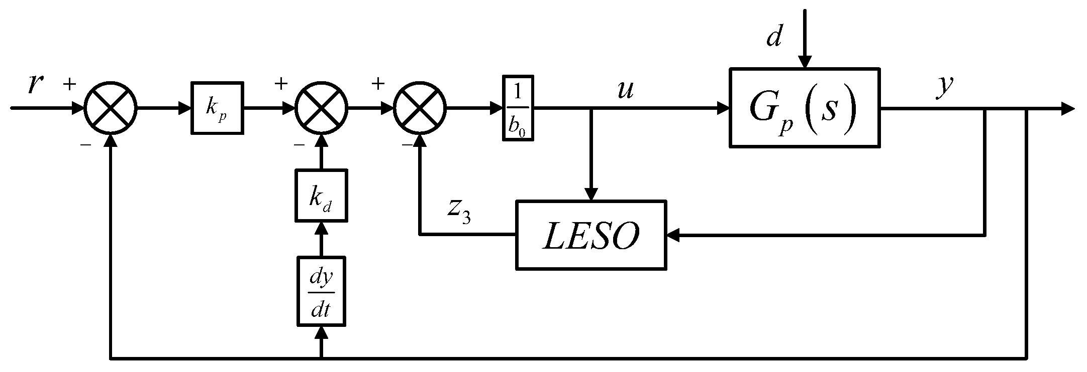
As mentioned above, $z_1$, $z_2$, $z_3$ are designed to track y, $\dot{y}$, f respectively. The core concept of LADRC is to approximate the entire system to a nth-order differential equation through estimating the system external and internal disturbance. Based on this approximation, PD control law can be easily designed to control the complex system. Although the expended state observer is proved to be stable in the long term, there still exists estimation error of state variables at the beginning of controlling process, which can adversely affect the controller performance. Therefore, it is of significantly practical and theoretical necessity to reduce the error of estimation. This paper recognizes that the LESO output $z_1$ and $z_2$, which respectively track the state y and $\dot{y}$, can be directly replaced by the system output y and the differential of y and the structure is as Figure 5. That is, the control law of (22) is replaced by (24). During this controlling process, the negative effect of the estimation error of $z_1$ and $z_2$ is avoided and the parameters only need to minimize the estimation error $z_3$, which reduces the stress of linear extended state observer and increases estimation accuracy. This modification can avoid the influence of estimation error of $z_1$ and $z_2$.

$$u_0=k_p(r-y)-k_d\dot{y}$$

(24)

Theoretically, the improved LADRC algorithm has stronger control ability with comparison of traditional LADRC algorithm, and simulation results will be analyzed in Section 4.

3.3. Supplementary Control of Aqua Electrolyzer

In the control process, it is impossible for AE to reduce its output while AE is operating at the point of zero, which will lead to degradation of system performance. Taking this situation into consideration, this paper proposes a supplementary control loop based on the original controller in Figure 6, where $u_C$ is the controller output, $u_{AE}$ is the final control output, and T is assumed to be 5 s. This control loop ensures that the output of AE can always operate at the setting point. The supplementary control loop effectively solves the aforementioned problem. More importantly, it widens the adjustment range of AE under any circumstances.

3.4. Parameter Optimization

Particle swarm optimization is widely used in optimization problems. And W. Liu et al. [27] propose the improved PSO based identification algorithm that can optimize parameters in real-time. However, for briefness, this paper employs GA-based PSO algorithm, which can avoid falling into local minima and obtain desirable parameters through searching in a wider range. The hybrid optimization algorithm includes the following six steps.

• Initialize all particles based on man-tuning parameters.
• Calculate the fitness value of the particles.
• Compare them to search for the best position pbest, choose the better half particles to the next generation and replace the rest half after genetic crossover operation.
• Update the position and velocity and find the best position gbest.
• Compare pbest with gbest and replace pbest by gbest if gbest is better. Then cycle.
• Stop the algorithm if the cycle time reaches 150 or turns to Step 3.

In order to accelerate optimization speed and enhance optimization efficiency, the fitness function is described by the rate of change of frequency (RoCoF) and the integral of time-weighted absolute value of the error (ITAE), and it is following (25)–(27).

$$ITAE=\int t|\Delta f|dt$$

(25)

$$RoCoF=\int t|\frac{df}{dt}|dt$$

(26)

$$FitnessValue=\int t|\Delta f|dt+\int t|\frac{df}{dt}|dt$$

(27)

The optimized parameters of improved LADRC, LADRC, PI and Fuzzy-PI controllers are given in

Table 4. The parameters of ILADRC controller used for simulation.

Diesel Generator			Aqua Electrolyzer			Fuel Cell
$b_0$	${\omega }_o$	${\omega }_c$	$b_0$	${\omega }_o$	${\omega }_c$	$b_0$	${\omega }_o$	${\omega }_c$
3.2270	8.4405	4.2164	73.8680	23.4958	5.7231	0.2379	14.6713	10.1203

,

Table 5. The parameters of LADRC controller used for simulation.

Diesel Generator			Aqua Electrolyzer			Fuel Cell
$b_0$	${\omega }_o$	${\omega }_c$	$b_0$	${\omega }_o$	${\omega }_c$	$b_0$	${\omega }_o$	${\omega }_c$
0.0503	11.0225	11.5792	19.0382	30.4135	7.5005	0.0490	30.1004	5.1474

and

Table 6. The parameters of PI and Fuzzy-PI controller used for simulation.

Diesel Generator		Aqua Electrolyzer		Fuel Cell
$k_p$	$k_i$	$k_p$	$k_i$	$k_p$	$k_i$
0.4395	12.9450	3.6890	14.4411	195.4674	209.2223

, respectively. The Fitness Value curve of ILADRC controller is presented in Figure 7.

3.5. The Overall Control Strategy of Microgrid Power System

Combined with the model described in Section 2 and the control strategy mentioned above, the overall control strategy of microgrid power system is depicted in Figure 8. Because of the excellent independence on the plant model and robustness of ILADRC, the general third-order ILADRC controller is employed as the controllers of DG, FC, and AE. While the system is in steady state, the deviation of frequency is expected to be 0, which means the set point of controller is 0. The frequency deviation $\Delta f$ is the input of ILADRC controller, which is equal to y in Figure 5. Through controlling the output of each energy sources to maintain the balance of active power output and load demand, the deviation of frequency can be stabilized to zero point.

4. Simulation Results and Analyses

In this section, the effectiveness of the proposed control strategy is verified by the following three simulation experiments. Microgrid power system is in steady state and each distributed unit is operating at setting point initially. All of the simulations are based on MATLAB/Simulink environment and the step time is 0.001s. The controller parameters are given in Table 4, Table 5 and Table 6.

4.1. Study on Load Power Change with Stable Wind Power

The simulations in this section are based on the model depicted in Figure 8. The controller block in Figure 8 adopts the general three-order LADRC controller described in Figure 5 with comparison of the general three-order ILADRC controller described in Figure 4, PI controller and Fuzzy-PI controller. In order to investigate the system performance with step change in load demand, the load power suddenly decreases from 1.0 p.u. to 0.8 p.u. at 1 s and increases from 0.8 p.u. to 1.0 p.u. at 1 s, respectively. And the output power of wind turbine generator is supposed to be stable.

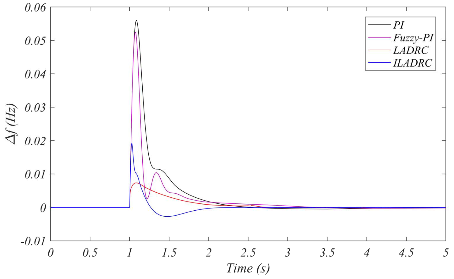
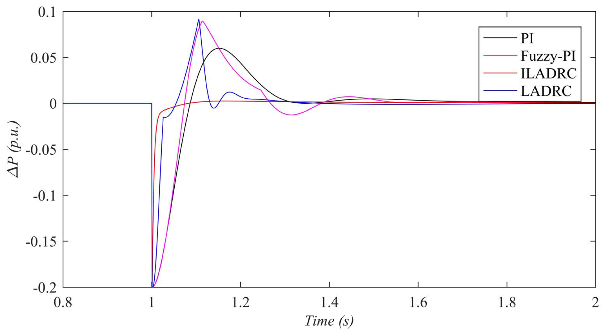
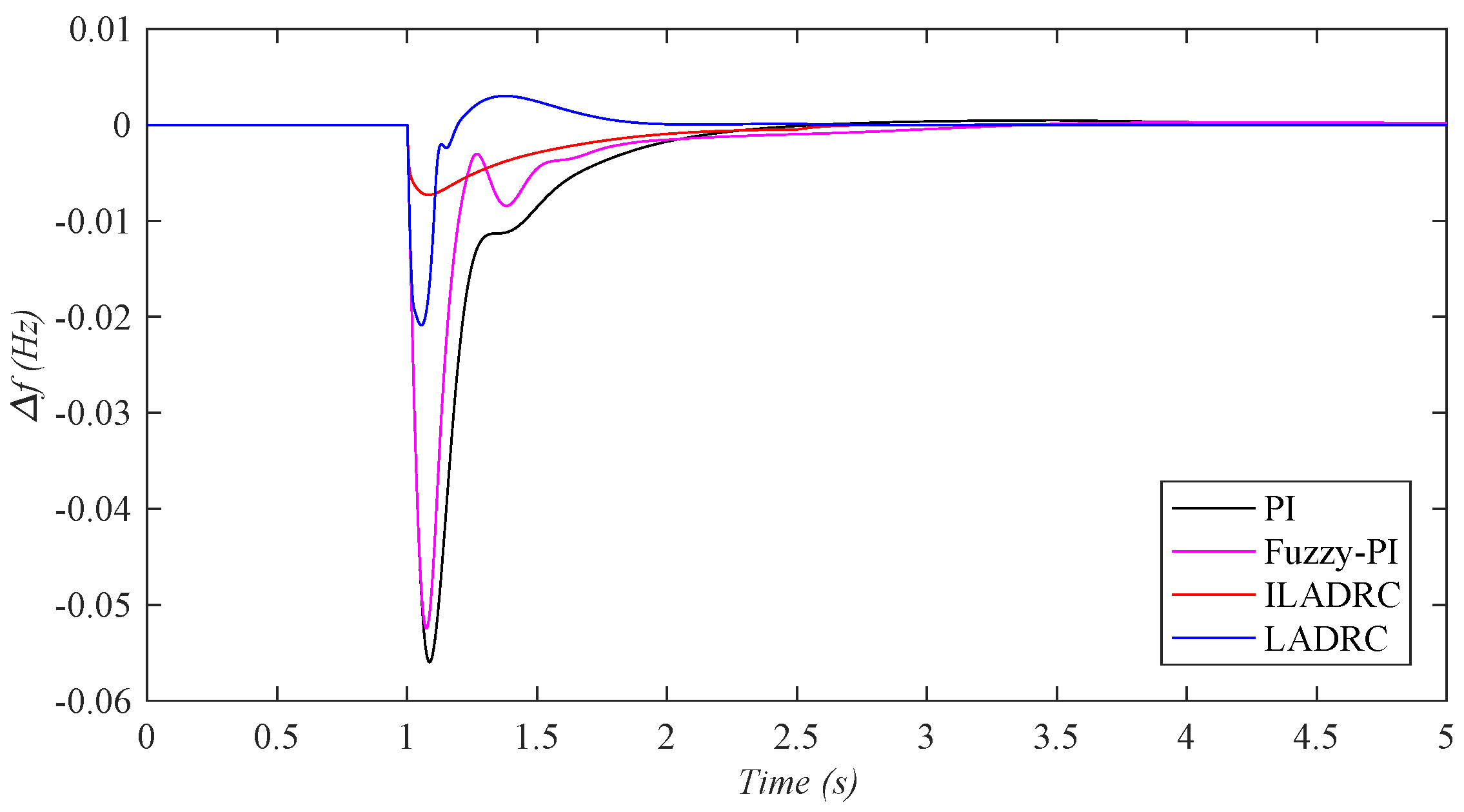
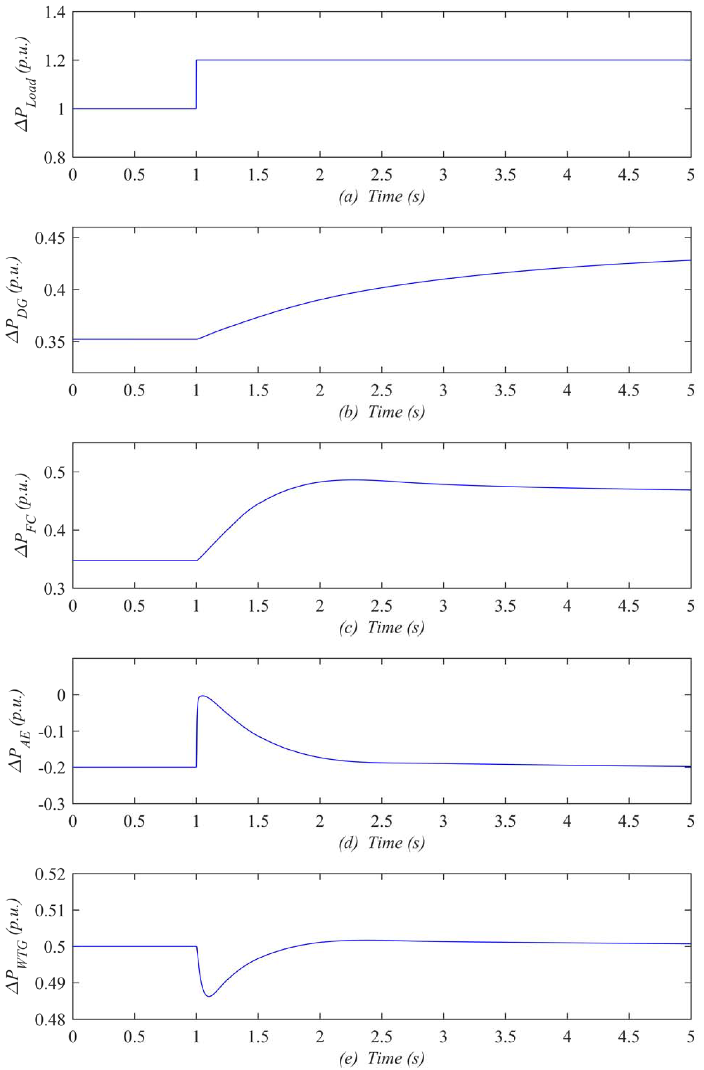
After the load demand decrease of 0.2 p.u. at 1 s, the transient response of system power exchange $\Delta P$ and system frequency deviation $\Delta f$ are described in Figure 9 and Figure 10, respectively. The comparison results of ILADRC, LADRC, PI and Fuzzy-PI are shown in

Table 7. Performance comparison with ILADRC, LADRC, PI and Fuzzy-PI controller.

Case	Controller	Overshoot	Settling Time	ITAE	RoCoF	ITAE + RoCoF
−0.2  p.u. Load Change	ILADRC	−0.0074 Hz	0.184 s	0.0092	0.0211	0.0303
	LADRC	−0.0192 Hz	0.260 s	0.0046	0.0449	0.0545
	Fuzzy-PI	−0.0525 Hz	0.470 s	0.0219	0.1317	0.1536
	PI	−0.0525 Hz	0.660  s	0.0169	0.1403	0.1572
+0.2  p.u. Load Change	ILADRC	0.0073 Hz	0.112 s	0.0081	0.0187	0.0268
	LADRC	0.0209 Hz	0.262 s	0.0045	0.0545	0.0590
	Fuzzy-PI	0.0525 Hz	0.484 s	0.1677	0.1314	0.1481
	PI	0.0560 Hz	0.659  s	0.0218	0.1316	0.1534

. With load demand decreasing, the overshoot value of ILADRC controller is −0.0074 Hz, which is considerably better than −0.0192 Hz, −0.0525 Hz and −0.0525 Hz derived by LADRC, Fuzzy-PI and PI controller, respectively. It can be obviously found that the settling time of frequency regulation based on ILADRC controller is reduced to 0.184 s and the sum of value of ITAE and RoCoF is reduced to 0.0303. All the simulation results declare the excellent performance of ILADRC controller. And the transient power responses of each energy sources based on ILADRC controller are depicted in Figure 11b–e. The simulation results with +0.2 p.u. change of load demand at 1 s are shown in Figure 12, Figure 13 and Figure 14 and Table 7, the analyses are the same to the above and this paper is not going to analyze them again.

4.2. Study on Load Power Change with Stochastic Wind Power

As aforementioned in Section 4.1, the simulations in this section are also based on the model depicted in Figure 8. The controller structure and parameters are following Figure 4 and Figure 5 and Table 4, Table 5 and Table 6. However, this case considers the stochastic characteristic of wind power and load demand.

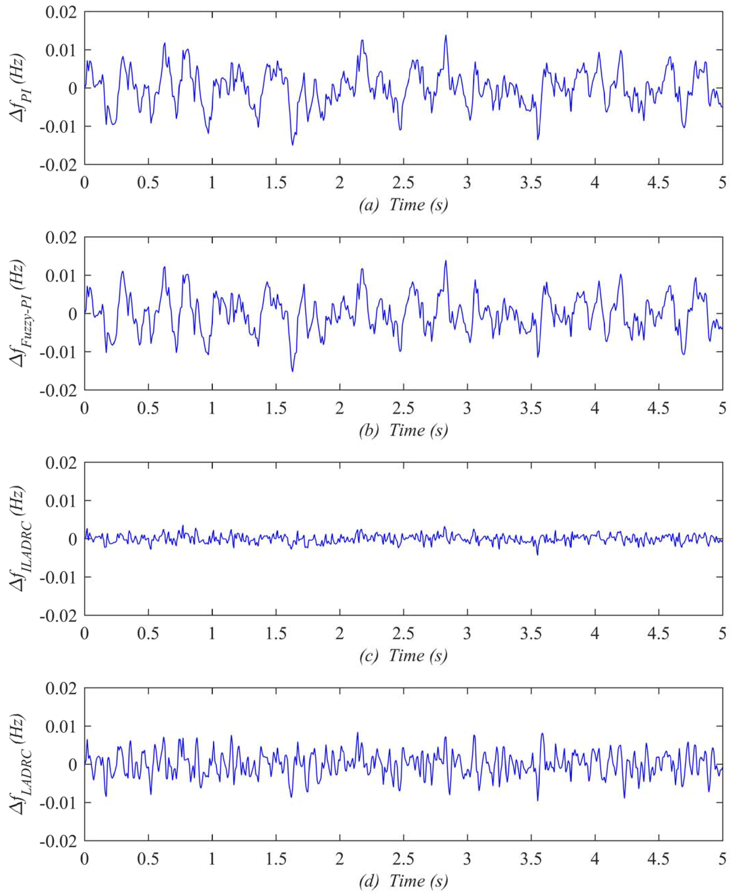
There are numerous unpredictable disturbances such as the randomness of wind speed and load power, which determines that the anti-disturbance ability is of significantly importance. First of all, the anti-disturbance analyses considering of stochastic $\Delta P_{WTG}$ and $\Delta P_L$ are studied. System frequency deviation $\Delta f$ with stochastic $\Delta P_{WTG}$ based on ILADRC, LADRC, PI and Fuzzy-PI controller are described in Figure 15a–d, respectively. And the stochastic characteristic of wind power and load demand are shown in Figure 16 and Figure 17, respectively. Same simulation results considering of the stochastic $\Delta P_L$ and both stochastic $\Delta P_{WTG}$ and $\Delta P_L$ are described in Figures Figure 18 and Figure 19, respectively. According to

Table 8. Comparison of the range of variation of $\Delta f$ with ILADRC, LADRC, PI and Fuzzy-PI controller under different disturbances.

Controller	The Range of Variation of $\mathbf{\Delta }\mathit{f}$
	With Stochastic ${\mathit{P}}_{\mathit{WTG}}$	With Stochastic ${\mathit{P}}_{\mathit{L}}$	With Stochastic ${\mathit{P}}_{\mathit{WTG}}$ and ${\mathit{P}}_{\mathit{L}}$
ILADRC	−0.0044 Hz∼0.0036 Hz	−0.0034 Hz∼0.0036 Hz	−0.0044 Hz∼0.0054 Hz
LADRC	−0.0097 Hz∼0.0084 Hz	−0.0070 Hz∼0.0065 Hz	−0.0104 Hz∼0.0102 Hz
Fuzzy-PI	−0.0150 Hz∼0.0139 Hz	−0.0097 Hz∼0.0095 Hz	−0.0172 Hz∼0.0189 Hz
PI	−0.0153 Hz∼0.0139 Hz	−0.0097 Hz∼0.0103 Hz	−0.0173 Hz∼0.0190 Hz

, the frequency fluctuation of microgrid system with the ILADRC is in an extremely smaller range than others, and average frequency fluctuation is also the smallest. It is obviously that the ILADRC controller has the best anti-disturbance capability.

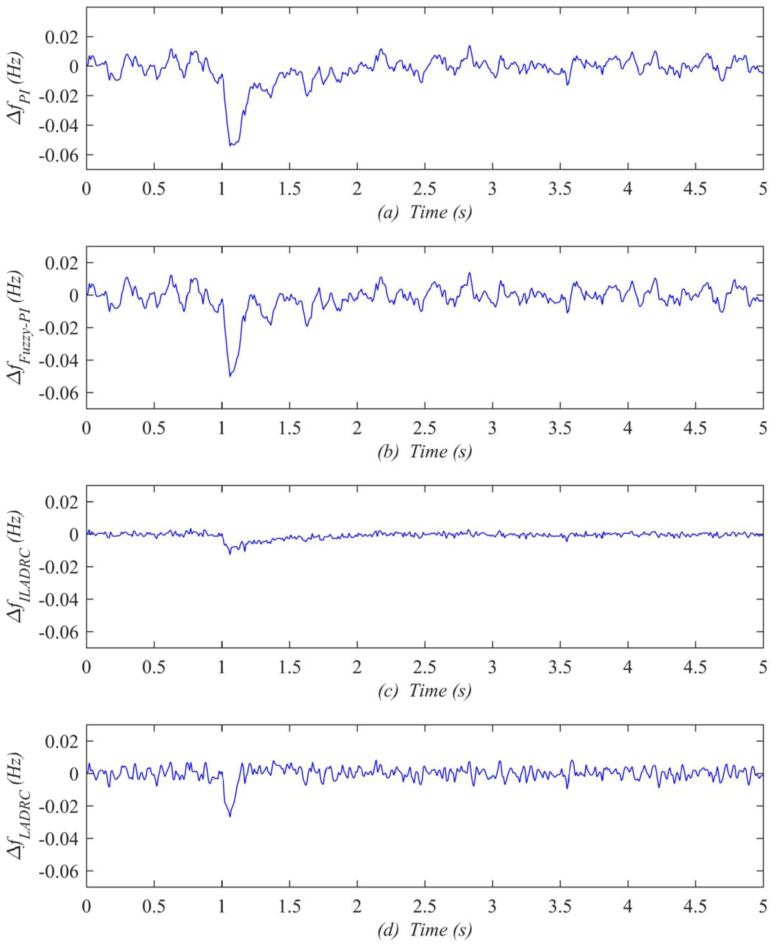
Furthermore, this paper researches the circumstance with stochastic power of wind turbine generator and +0.2 p.u. change of load demand at 1 s. The simulation results are presented in Figure 20 and

Table 9. Performance comparison with ILADRC, LADRC, PI and Fuzzy-PI controller under stochastic power of wind turbine generator and +0.2 p.u. change of load demand.

Controller	Overshoot	ITAE
ILADRC	−0.0127 Hz	0.0131
LADRC	−0.0269 Hz	0.0304
Fuzzy-PI	−0.0503 Hz	0.0551
PI	−0.0542 Hz	0.0551

. It is easy to observe that the performance of ILADRC controller is better than others. Its overshoot −0.0127 Hz and ITAE 0.0131 are both better than those with LADRC, Fuzzy-PI and PI. However, the value of RoCoF is meaningless because the stochastic characteristic of wind power can cause tremendous variability of frequency and power.

4.3. Robustness Analysis

Based on the aforementioned system model and control strategy, this section studies the robustness capability of ILADRC algorithm. The complexity and uncertainty of the microgrid composition determines that the parameters of the microgrid system may vary within an uncertainty range. And if the controller is difficult to deal with the variety of parameters, undesirable challenges and even collapse will be encountered. Consequently, it is of great importance to evaluate the ability of the system to tackle this situation. As previously analyzed, Monte-Carlo experiment is carried out to verify the robustness of system. With system parameter M and D variation within 10% for 200 times, the simulation results are presented in Figure 21. The changes of system with the ILADRC approach is almost negligible. However, traditional LADRC, Fuzzy-PI and PI based system have wider distribution. The result indicates that the ILADRC has better robustness capability.

5. Conclusions

This paper studies on the microgrid power system with configuration of variable-speed wind turbine generator, diesel generator, fuel cell, aqua electrolyzer and load demand. The ILADRC algorithm can greatly improve the stability and robustness of system. Furthermore, the supplementary control loop of aqua electrolyzer is also proposed to enhance system control ability. And the parameters of controllers are optimized by GA-based PSO algorithm. Then, in order to increase the optimization efficiency, this paper adopts the sum of the rate of change of frequency (RoCoF) and the integral of time-weighted absolute value of the error (ITAE) to be the fitness value. Adequate simulation experiments are completed to demonstrate the effectiveness of the proposed algorithm and the results indicate that improved LADRC controller can provide better performances comparing with traditional LADRC, PI and Fuzzy-PI controller. Moreover, the results also reveal the capability of anti-disturbance and excellent robustness of system with the proposed ILADRC algorithm.

Nowadays, DC microgrid is demonstrating the advantages over AC microgrid [28]. The higher system efficiency, higher system stability, and lower system cost make DC microgrid become an increasingly popular solution for small-scale power systems. Theoretically, the proposed ILADRC algorithm in this paper also has the potential to be adopted into DC microgrid. Moreover, because of the interaction between frequency regulation and voltage regulation, it is meaningful to take consideration of this situation in the future work.

References

- Palizban, O.; Kauhaniemi, K.; Guerrero, J.M. Microgrids in active network management—Part II: System operation, power quality and protection. Renew. Sustain. Energy Rev. 2014, 36, 440–451. [Google Scholar] [CrossRef]
- Olivares, D.E.; Mehrizi-Sani, A.; Etemadi, A.H.; Canizares, C.A. Trends in microgrid control. IEEE Trans. Smart Grid 2014, 5, 1905–1919. [Google Scholar] [CrossRef]
- Pandey, S.K.; Mohanty, S.R.; Kishor, N. A literature survey on load–frequency control for conventional and distribution generation power systems. Renew. Sust. Energy Rev. 2013, 25, 318–334. [Google Scholar] [CrossRef]
- Senjyu, T.; Nakaji, T.; Uezato, K.; Funabashi, T. A hybrid power system using alternative energy facilities in isolated island. IEEE Trans. Energy Convers. 2005, 20, 406–414. [Google Scholar] [CrossRef]
- Lee, D.J.; Wang, L. Small-signal stability analysis of an autonomous hybrid renewable energy power generation/energy storage system part I: Time-domain simulations. IEEE Trans. Energy Convers. 2008, 23, 311–320. [Google Scholar] [CrossRef]
- Nayeripour, M.; Hoseintabar, M.; Niknam, T. Frequency deviation control by coordination control of FC and double-layer capacitor in an autonomous hybrid renewable energy power generation system. Renew. Energy 2011, 36, 1741–1746. [Google Scholar] [CrossRef]
- Das, D.C.; Roy, A.K.; Sinha, N. GA based frequency controller for solar thermal–diesel–wind hybrid energy generation/energy storage system. Int. J. Electron. Power Energy Syst. 2012, 43, 262–279. [Google Scholar] [CrossRef]
- Bevrani, H.; Habibi, F.; Babahajyani, P.; Watanabe, M. Intelligent Frequency Control in an AC Microgrid: Online PSO-Based Fuzzy Tuning Approach. IEEE Trans. Smart Grid 2012, 3, 1935–1944. [Google Scholar] [CrossRef]
- Sekhar, P.C.; Mishra, S. Storage free smart energy management for frequency control in a diesel-pv-fuel cell-based hybrid AC microgrid. IEEE Trans. Neural Netw. Learn. Syst. 2016, 27, 1657–1671. [Google Scholar] [CrossRef] [PubMed]
- Sekhar, P.C.; Mishra, S. Sliding mode based feedback linearizing controller for grid connected multiple fuel cells scenario. Int. J. Electron. Power Energy Syst. 2014, 60, 190–202. [Google Scholar] [CrossRef]
- Liu, W.; Gu, W.; Sheng, W.; Meng, X.; Wu, Z.; Chen, W. Decentralized Multi-Agent System-Based Cooperative Frequency Control for Autonomous Microgrids With Communication Constraints. IEEE Trans. Sustain. Energy 2014, 5, 446–456. [Google Scholar] [CrossRef]
- Dong, L.; Zhang, Y.; Gao, Z. A robust decentralized load frequency controller for interconnected power system. ISA Trans. 2012, 51, 410–419. [Google Scholar] [CrossRef] [PubMed]
- Yan, B.; Tian, Z.; Shi, S.; Weng, Z. Fault diagnosis for a class of nonlinear systems via ESO. ISA Trans. 2008, 47, 386–394. [Google Scholar] [CrossRef] [PubMed]
- Tang, Y.; Bai, Y.; Huang, C.-Z.; Du, B. Linear active disturbance rejection-based load frequency control concerning high penetration of wind energy. Energy Convers. Manag. 2015, 95, 259–271. [Google Scholar] [CrossRef]
- Kaur, A.; Kaushal, J.; Basak, P. A review on microgrid central controller. Renew. Sustain. Energy Review. 2016, 55, 338–345. [Google Scholar] [CrossRef]
- Aouali, F.Z.; Becherif, M.; Ramadan, H.S.; Emziane, M.; Khellaf, A.; Mohammedi, K. Analytical modelling and experimental validation of proton exchange membrane electrolyzer for hydrogen production. Int. J. Hydrogen Energy 2017, 42, 1366–1374. [Google Scholar] [CrossRef]
- Sanz-Bermejo, J.; Muñoz-Antón, J.; Gonzalez-Aguilar, J.; Romero, M. Part load operation of a solid oxide electrolysis system for integration with renewable energy sources. Int. J. Hydrogen Energy 2015, 40, 8291–8303. [Google Scholar] [CrossRef]
- Zhu, Y.; Tomsovic, K. Development of models for analyzing the load-following performance of microturbines and fuel cells. Electron. Power Syst. Res. 2002, 62, 1–11. [Google Scholar] [CrossRef]
- Dreidy, M.; Mokhlis, H.; Mekhilef, S. Inertia response and frequency control techniques for renewable energy sources: A review. Renew. Sustain. Energy Rev. 2017, 69, 144–155. [Google Scholar] [CrossRef]
- Bonfiglio, A.; Delfino, F.; Invernizzi, M.; Procopio, R. Modeling and Maximum Power Point Tracking Control of Wind Generating Units Equipped with Permanent Magnet Synchronous Generators in Presence of Losses. Energies 2017, 10, 102. [Google Scholar] [CrossRef]
- Gonzalez-Longatt, F.M.; Bonfiglio, A.; Procopio, R.; Verduci, B. Evaluation of inertial response controllers for full-rated power converter wind turbine (Type 4). In Proceedings of the IEEE Power and Energy Society General Meeting, Boston, MA, USA, 17–21 July 2016; pp. 1944–9933. [Google Scholar]
- Mauricio, J.M.; Marano, A.; Gomez-Exposito, A.; Martinez Ramos, J.L. Frequency regulation controbution through variable-speed wind energy conversion systems. IEEE Trans. Power Syst. 2009, 24, 173–180. [Google Scholar] [CrossRef]
- Modirkhazeni, A.; Almasi, O.N.; Khooban, M.H. Improved frequency dynamic in isolated hybrid power system using an intelligent method. Int. J. Electron. Power Energy Syst. 2016, 78, 225–238. [Google Scholar] [CrossRef]
- Bhatt, P.; Ghoshal, S.P.; Roy, R. Coordinated control of TCPS and SMES for frequency regulation of interconnected restructured power systems with dynamic participation from DFIG based wind farm. Renew. Energy 2012, 40, 40–50. [Google Scholar] [CrossRef]
- Chai, S.J.; Li, D.H.; Yao, X.L. Active disturbance rejection controller for high-order system. In Proceedings of the 2011 30th Chinese Control Conference, Yantai, China, 22–24 July 2011; pp. 3798–3802. [Google Scholar]
- Gao, Z.Q. Active disturbance rejection control: A paradigm shift in feedback control system design. In Proceedings of the 2006 American Control Conference, Minneapolis, MN, USA, 14–16 June 2006; pp. 2399–2405. [Google Scholar]
- Liu, W.; Liu, L.; Chung, I.Y.; Cartes, D.A. Real-time particle swarm optimization based parameter identification applied to permanent magnet synchronous machine. Appl. Soft Comput. 2011, 11, 2556–2564. [Google Scholar] [CrossRef]
- Han, Y.; Chen, W.; Li, Q. Energy Management Strategy Based on Multiple Operating States for a Photovoltaic/Fuel Cell/Energy Storage DC Microgrid. Energies 2017, 10, 136. [Google Scholar] [CrossRef]
Figure 1.
Islanded AC Microgrid Power System.