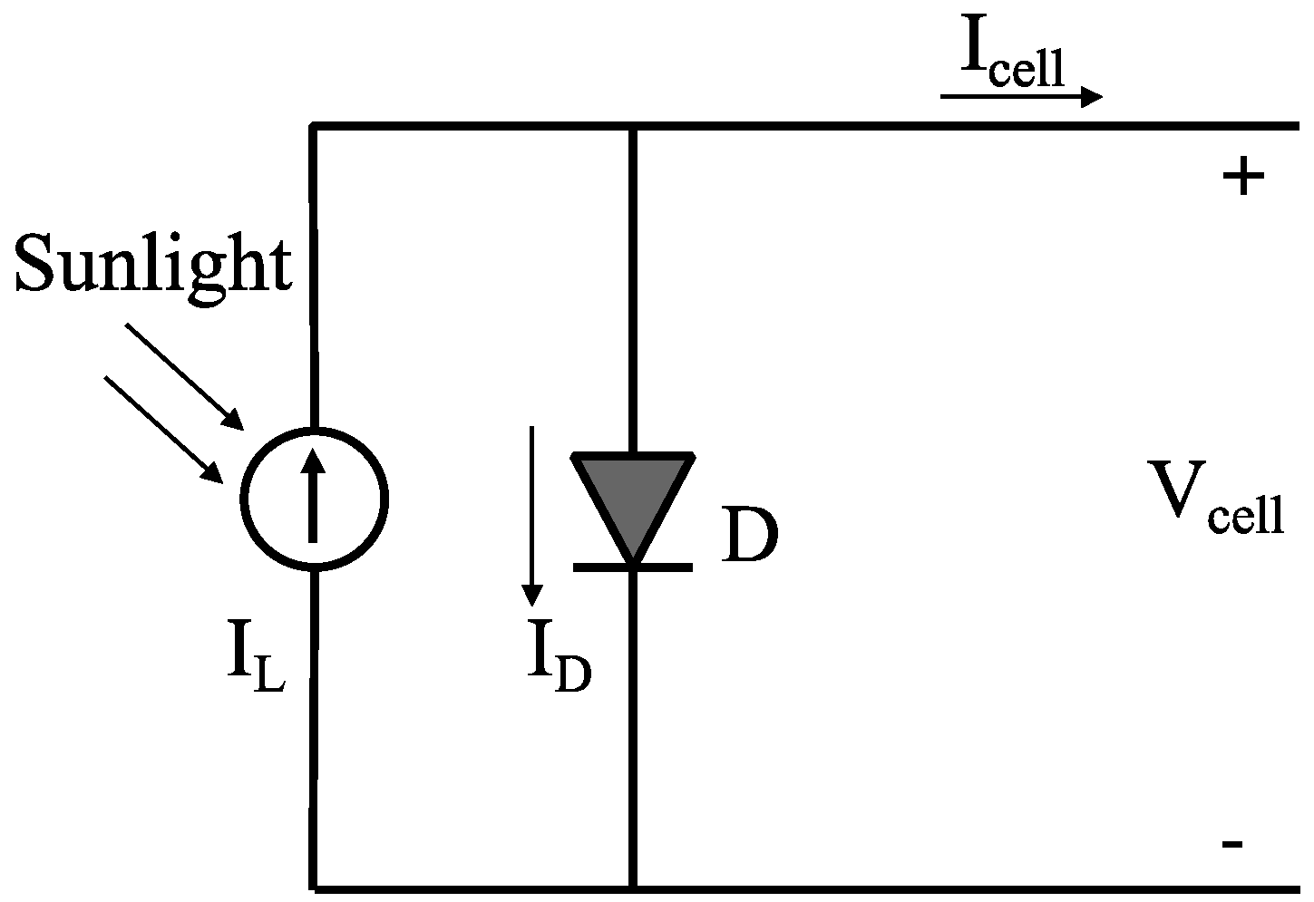
Figure 1.
Ideal circuit model of a photovoltaic cell.
Figure 1.
Ideal circuit model of a photovoltaic cell.
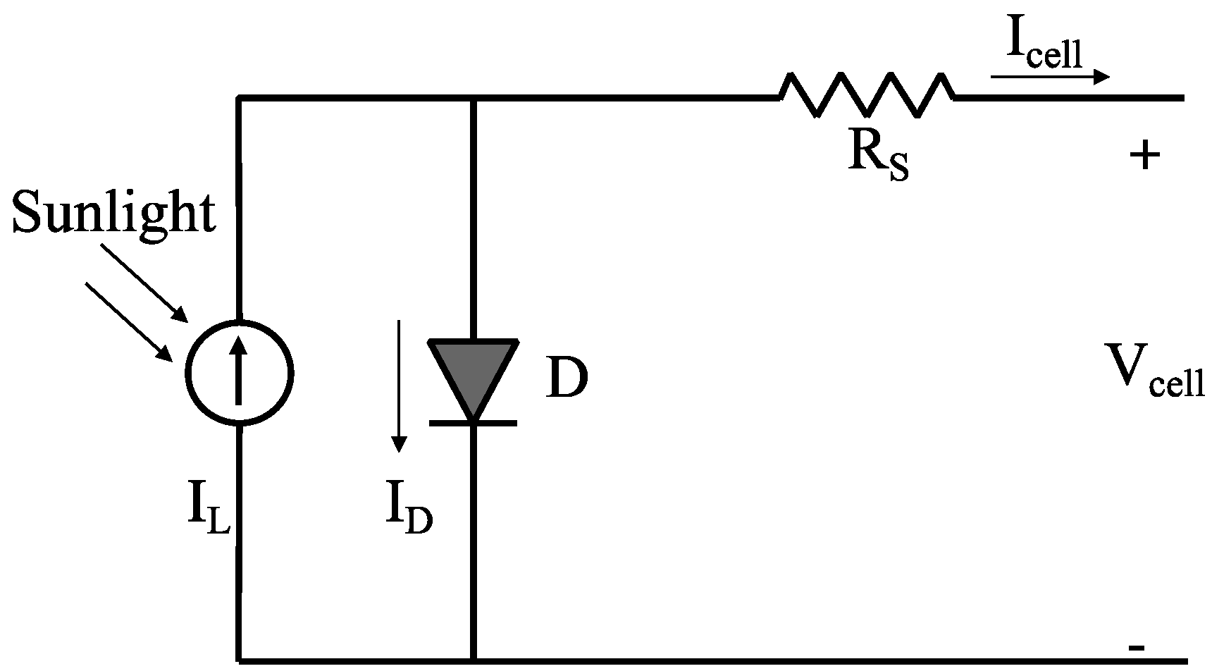
Figure 2.
Single-Diode model of a photovoltaic cell, showing the added lumped series resistor .
Figure 2.
Single-Diode model of a photovoltaic cell, showing the added lumped series resistor .
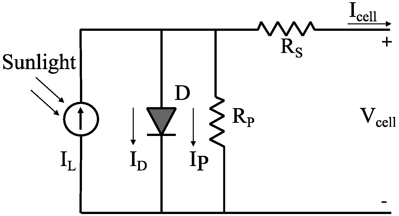
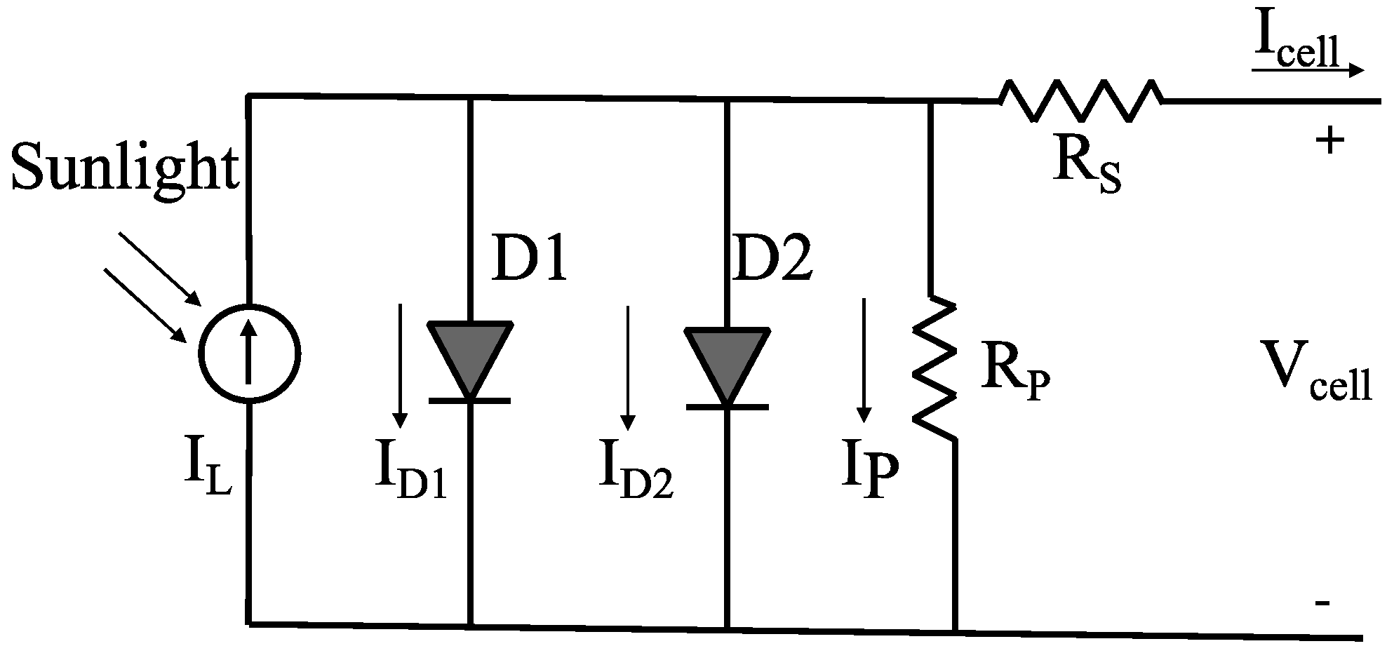
Figure 3.
Single-diode model of a photovoltaic cell, which includes both a lumped series resistor and a shunt resistor .
Figure 3.
Single-diode model of a photovoltaic cell, which includes both a lumped series resistor and a shunt resistor .
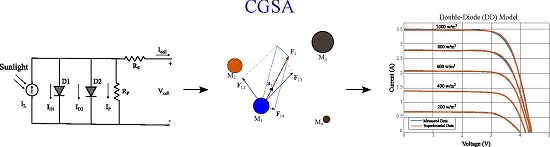
Figure 4.
Double-diode model of a photovoltaic cell.
Figure 4.
Double-diode model of a photovoltaic cell.
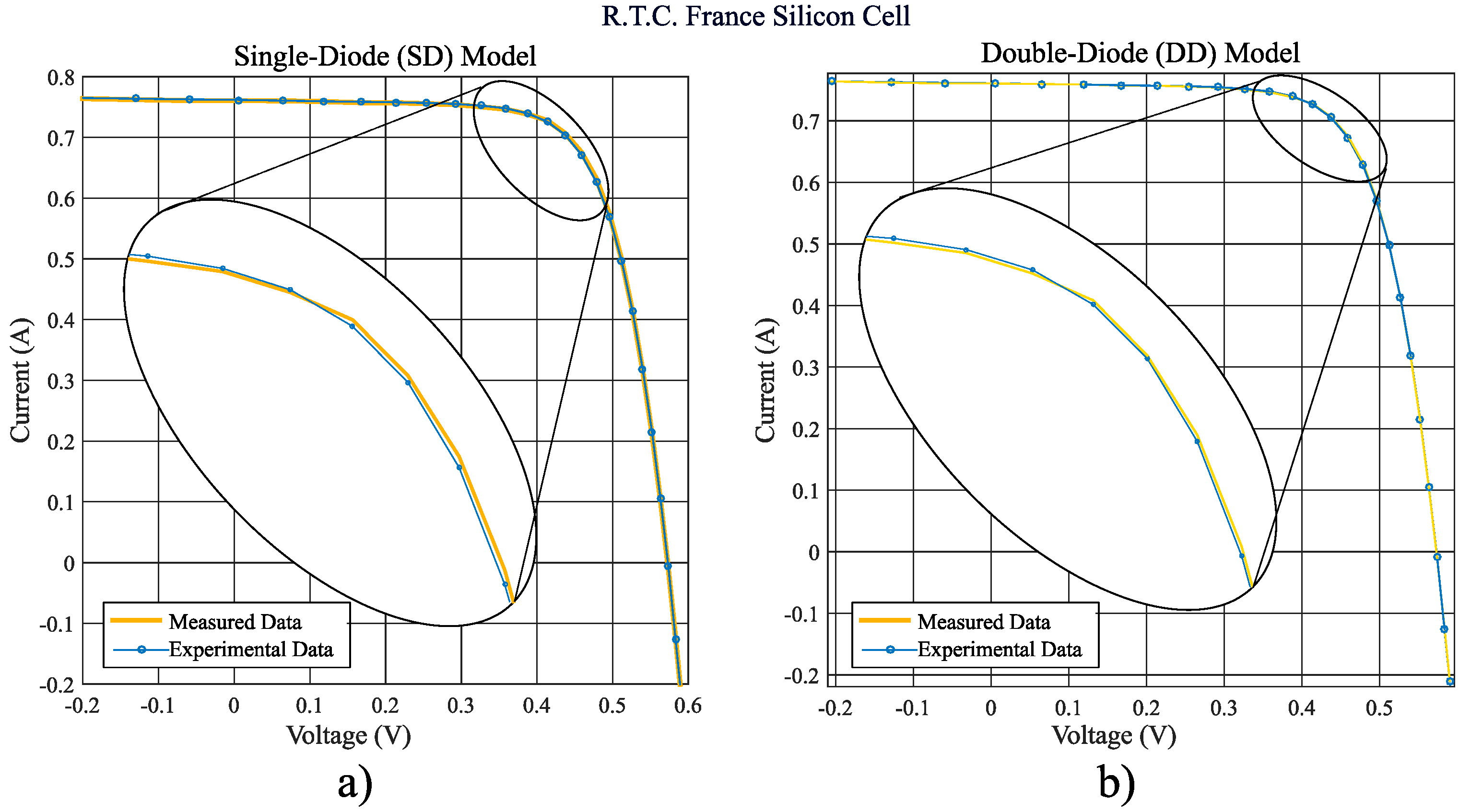
Figure 5.
PV Cell’s measured and estimated I-V characteristics for (a) SD model and (b) DD model under specific test conditions ( and ).
Figure 5.
PV Cell’s measured and estimated I-V characteristics for (a) SD model and (b) DD model under specific test conditions ( and ).
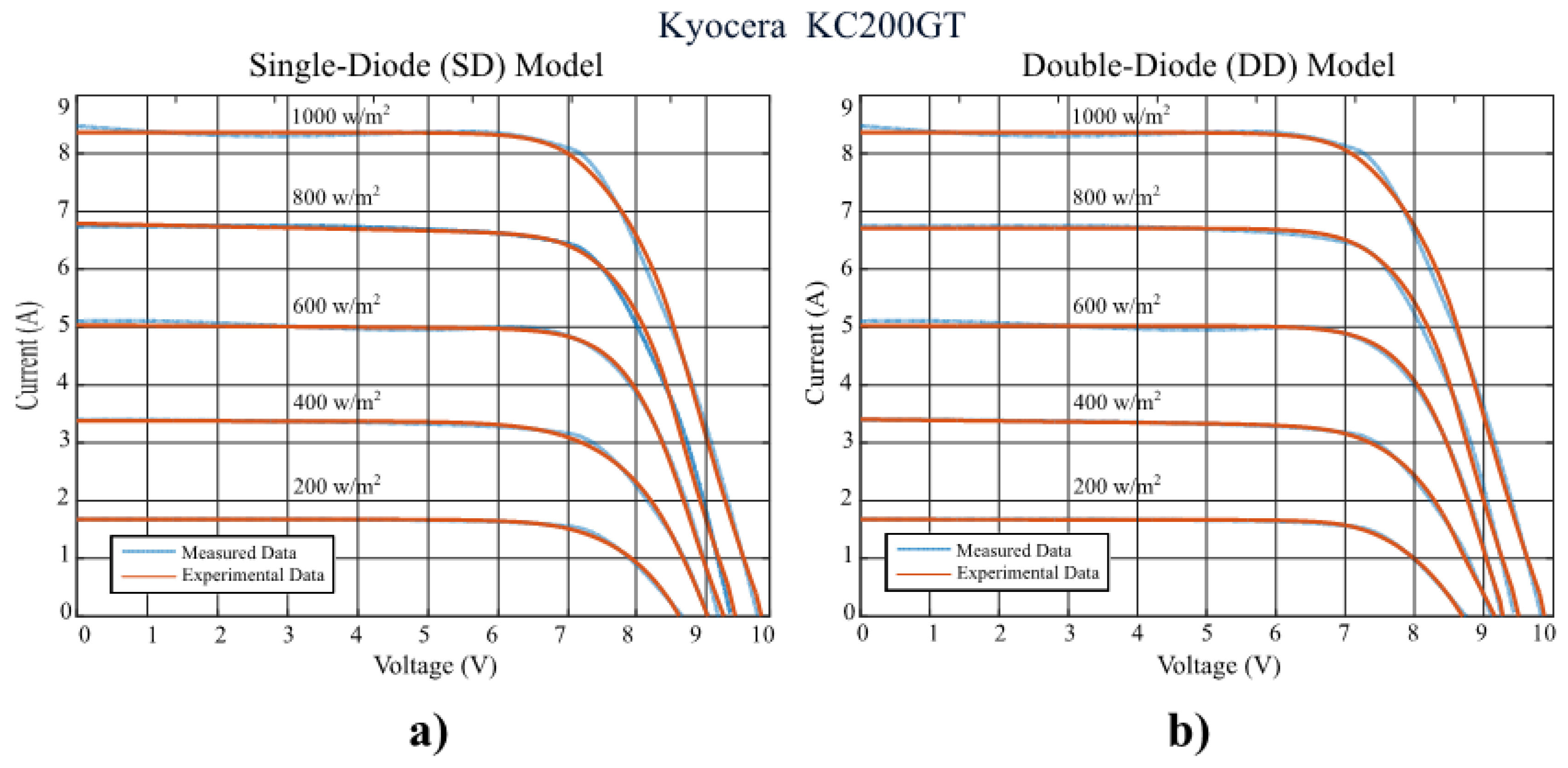
Figure 6.
Estimated I-V characteristics curves at different irradiance levels (200, 400, 600, 800 and 1000 ) and fixed cell temperature ( ) for an individual cell from a Kyocera KC200GT Solar Panel. (a) SD model and (b) DD model.
Figure 6.
Estimated I-V characteristics curves at different irradiance levels (200, 400, 600, 800 and 1000 ) and fixed cell temperature ( ) for an individual cell from a Kyocera KC200GT Solar Panel. (a) SD model and (b) DD model.
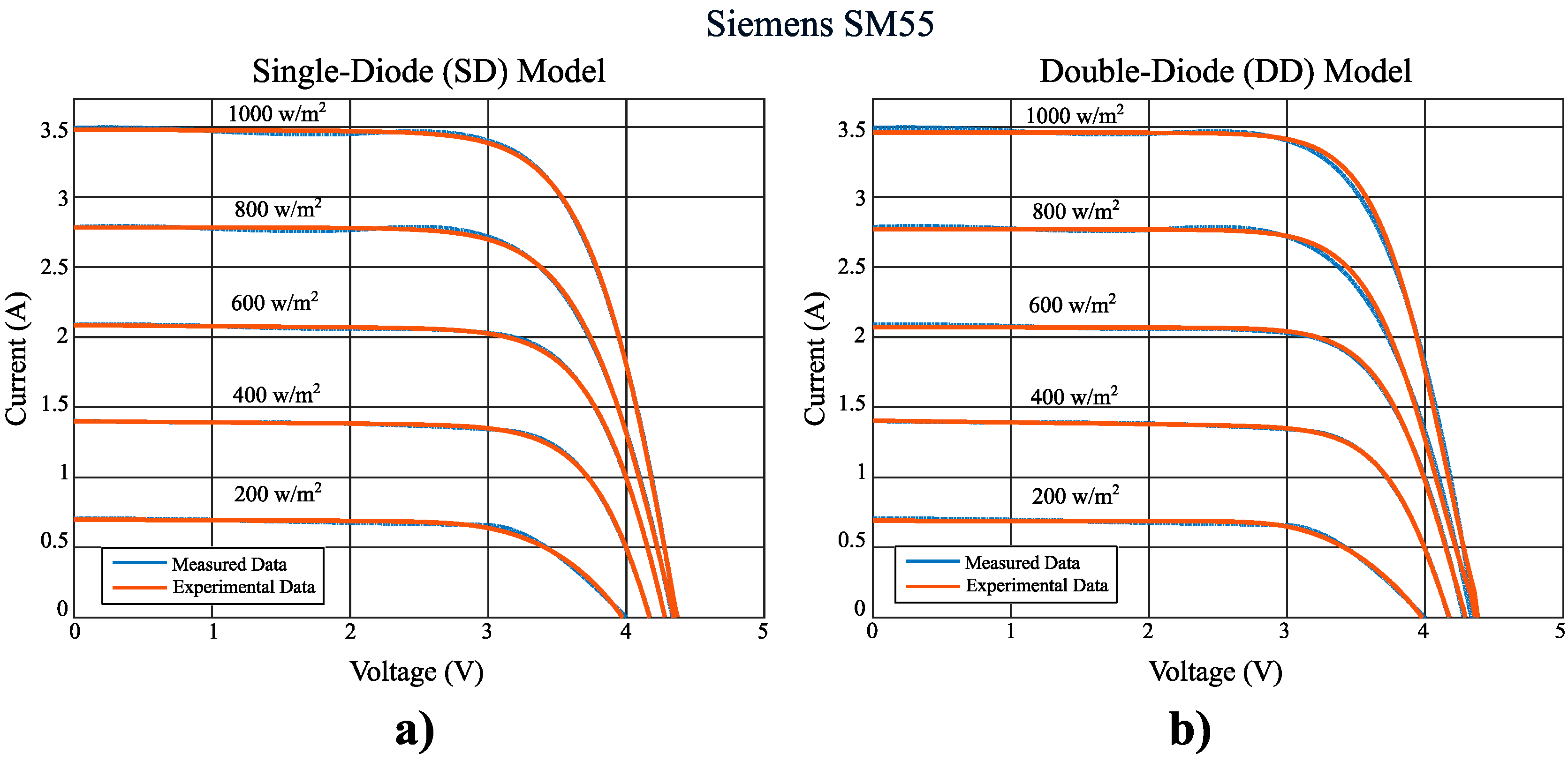
Figure 7.
Estimated I-V characteristics curves at different irradiance levels (200, 400, 600, 800 and 1000 ) and fixed cell temperature ( ) for an individual cell from a Siemens SM55 Solar Panel. (a) SD model and (b) DD model.
Figure 7.
Estimated I-V characteristics curves at different irradiance levels (200, 400, 600, 800 and 1000 ) and fixed cell temperature ( ) for an individual cell from a Siemens SM55 Solar Panel. (a) SD model and (b) DD model.
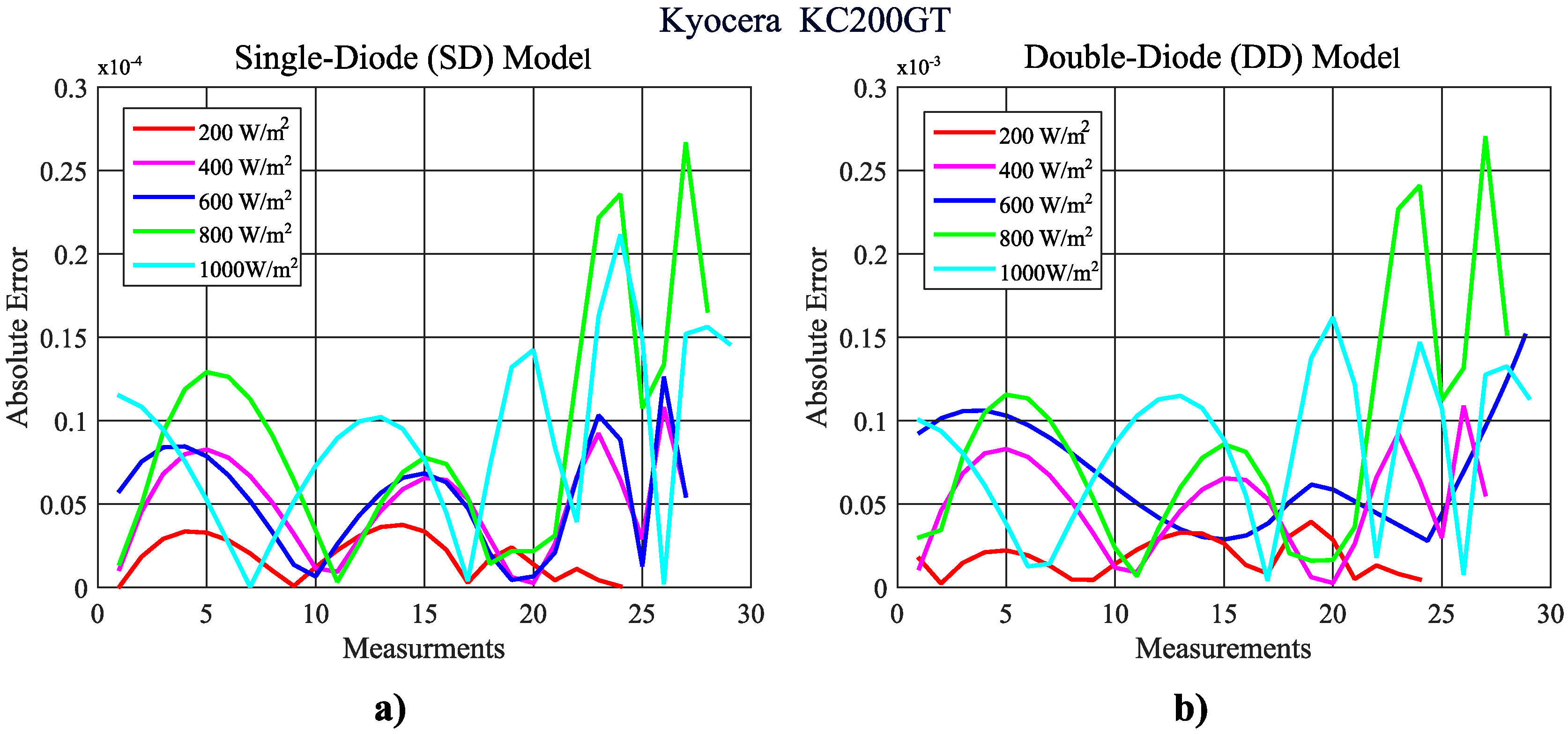
Figure 8.
Absolute error curves between the measured and experimental I-V data at different irradiance levels (200, 400, 600, 800 and 1000 ) and fixed cell temperature ( ) for an individual cell from a Kyocera KC200GT Solar Panel. (a) SD model and (b) DD model.
Figure 8.
Absolute error curves between the measured and experimental I-V data at different irradiance levels (200, 400, 600, 800 and 1000 ) and fixed cell temperature ( ) for an individual cell from a Kyocera KC200GT Solar Panel. (a) SD model and (b) DD model.
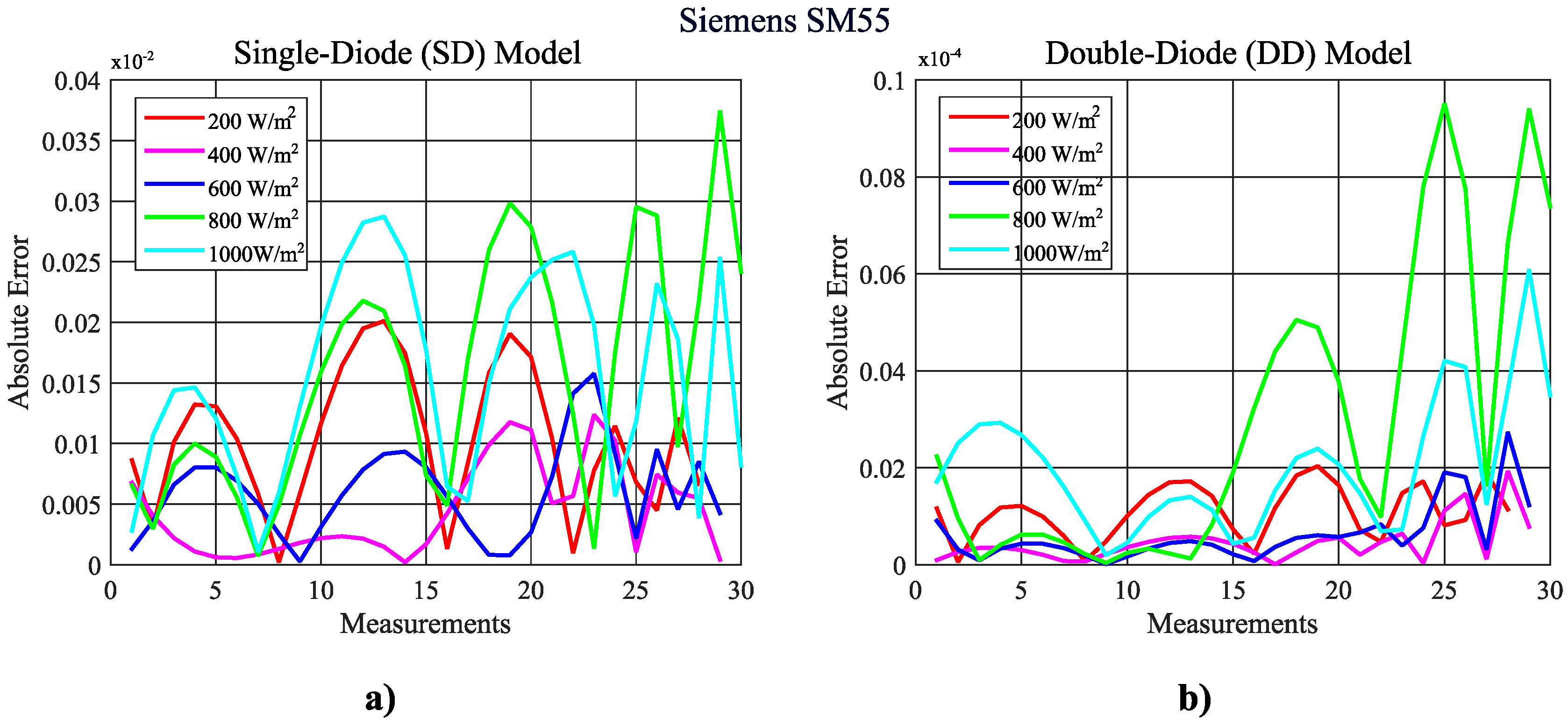
Figure 9.
Absolute error curves between the measured and experimental I-V data at different irradiance levels (200, 400, 600, 800 and 1000 ) and fixed cell temperature ( ) for an individual cell from a Siemens SM55 Solar Panel. (a) SD model and (b) DD model.
Figure 9.
Absolute error curves between the measured and experimental I-V data at different irradiance levels (200, 400, 600, 800 and 1000 ) and fixed cell temperature ( ) for an individual cell from a Siemens SM55 Solar Panel. (a) SD model and (b) DD model.
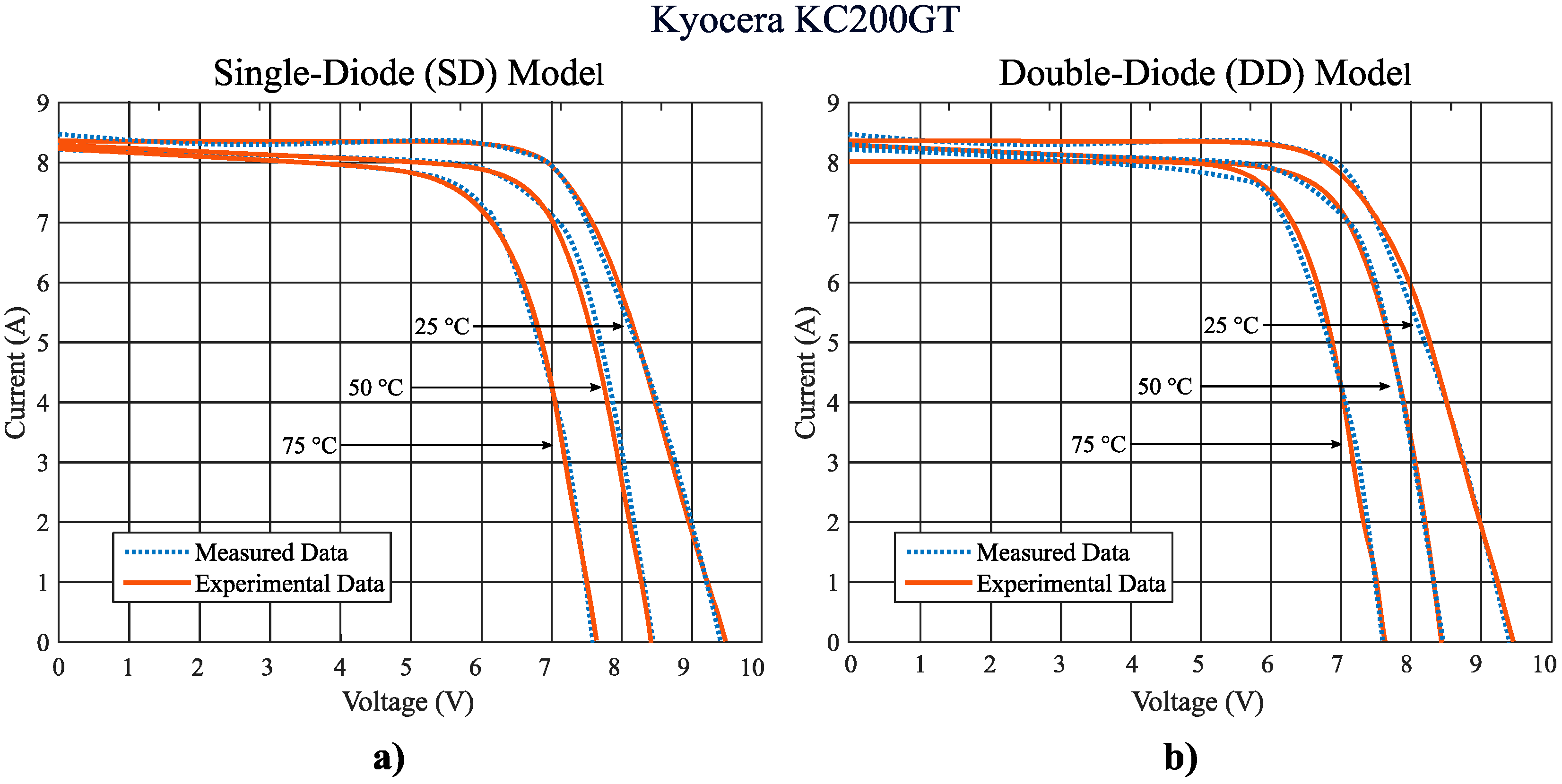
Figure 10.
Estimated I-V characteristics curves at different cell temperatures (25, 50 and 75 ) and fixed solar irradiance ( ) for an individual cell from a Kyocera KC200GT Solar Panel. (a) SD model and (b) DD model.
Figure 10.
Estimated I-V characteristics curves at different cell temperatures (25, 50 and 75 ) and fixed solar irradiance ( ) for an individual cell from a Kyocera KC200GT Solar Panel. (a) SD model and (b) DD model.
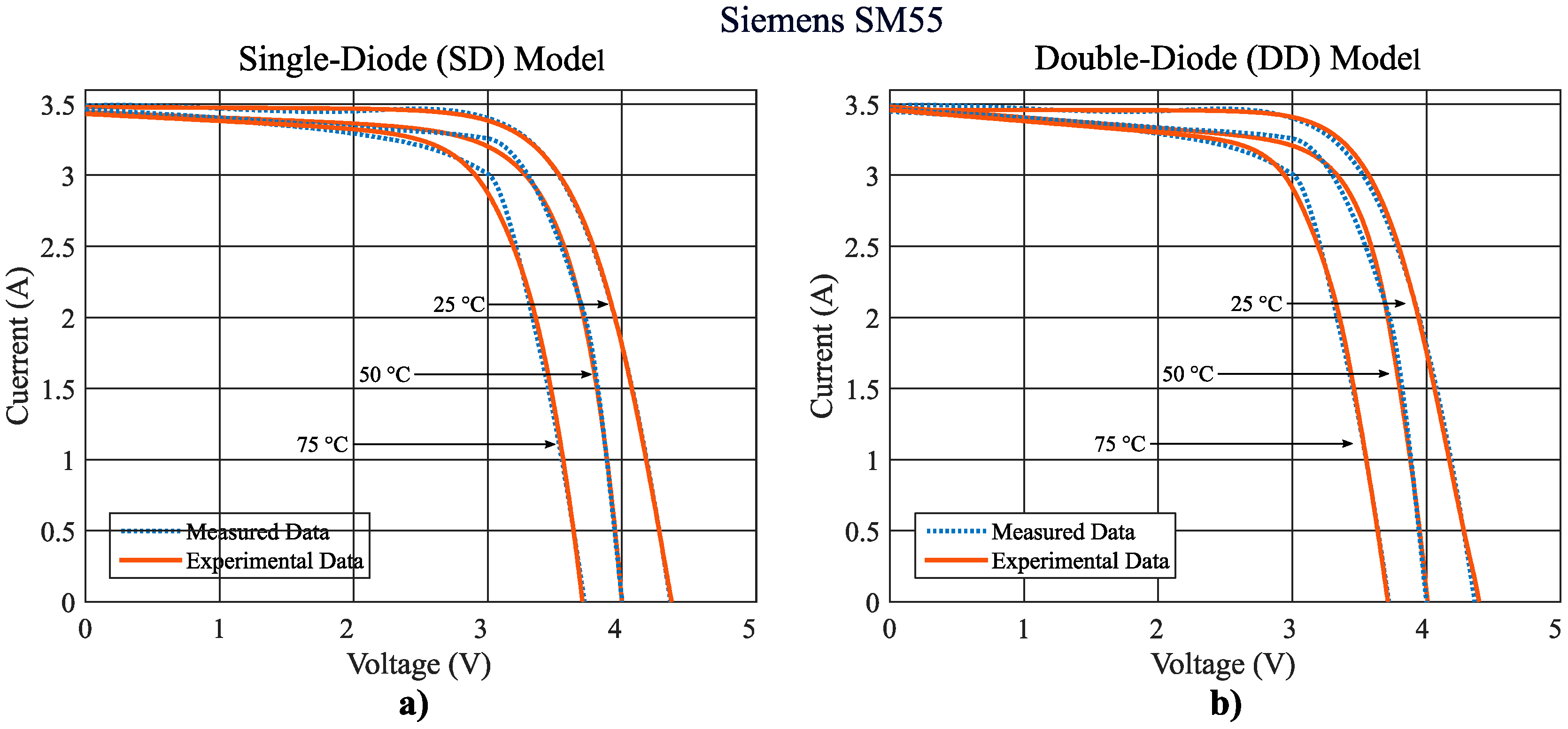
Figure 11.
Estimated I-V characteristics curves at different cell temperatures (25, 50 and 75 ) and fixed solar irradiance ( ) for an individual cell from a Kyocera KC200GT Solar Panel. (a) SD model and (b) DD model.
Figure 11.
Estimated I-V characteristics curves at different cell temperatures (25, 50 and 75 ) and fixed solar irradiance ( ) for an individual cell from a Kyocera KC200GT Solar Panel. (a) SD model and (b) DD model.
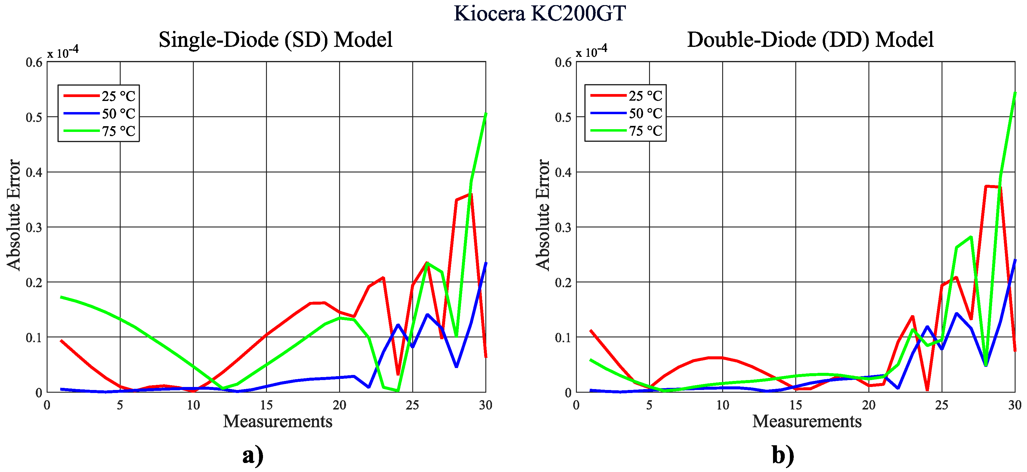
Figure 12.
Absolute error curves between the measured and experimental I-V data at different cell temperatures (25, 50 and 75 ) and fixed solar irradiance ( ) for an individual cell from a Kyocera KC200GT Solar Panel. (a) SD model and (b) DD model.
Figure 12.
Absolute error curves between the measured and experimental I-V data at different cell temperatures (25, 50 and 75 ) and fixed solar irradiance ( ) for an individual cell from a Kyocera KC200GT Solar Panel. (a) SD model and (b) DD model.
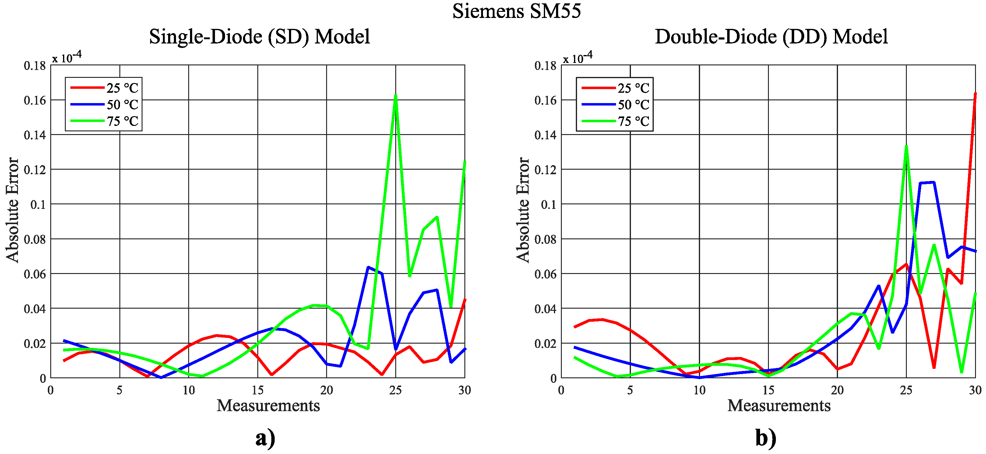
Figure 13.
Absolute error curves between the measured and experimental I-V data at different cell temperatures (25, 50 and 75 ) and fixed solar irradiance ( ) for an individual cell from a Siemens SM55 Solar Panel. (a) SD model and (b) DD model.
Figure 13.
Absolute error curves between the measured and experimental I-V data at different cell temperatures (25, 50 and 75 ) and fixed solar irradiance ( ) for an individual cell from a Siemens SM55 Solar Panel. (a) SD model and (b) DD model.
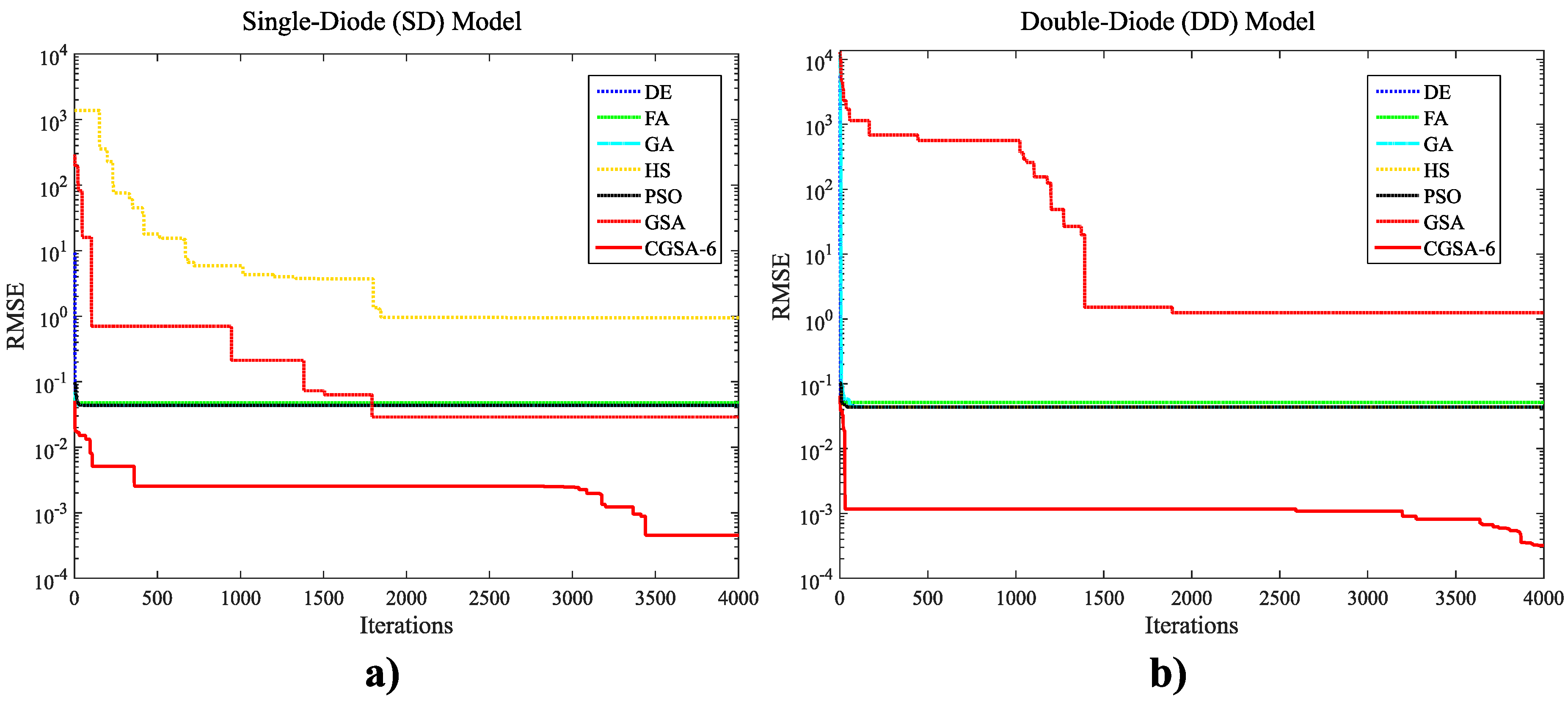
Figure 14.
Evolution curves for (a) SD Model and (b) DD Model, obtained by applying DE, FA, GA, HS, PSO, GSA and CGSA-6.
Figure 14.
Evolution curves for (a) SD Model and (b) DD Model, obtained by applying DE, FA, GA, HS, PSO, GSA and CGSA-6.
Table 1.
CGSA minimization results for the SD and DD models (with and ), for 30 individual runs (with iterations each and search agents). Note that the best outcomes for each of the simulated solar cell models are boldfaced.
Table 1.
CGSA minimization results for the SD and DD models (with and ), for 30 individual runs (with iterations each and search agents). Note that the best outcomes for each of the simulated solar cell models are boldfaced.
| Method | Embedded Chaotic Map () | Single-Diode (SD) Model | Double-Diode (DD) Model |
|---|
| | | | | |
|---|
| CGSA-1 | (Chebyshev) | 4.38 | 3.41 | 5.58 | 12.7 | 10.3 | 4.99 |
| CGSA-2 | (Circle) | 2.77 | 1.60 | 6.69 | 40.6 | 52.4 | 6.81 |
| CGSA-3 | (Gauss/Mouse) | 1.34 | 3.38 | 1.23 | 53.9 | 53.9 | 4.12 |
| CGSA-4 | (Iterative) | 7.31 | 8.98 | 6.27 | 39.6 | 41.7 | 5.23 |
| CGSA-5 | (Logistic) | 1.34 | 1.24 | 5.94 | 92.6 | 87.9 | 1.68 |
| CGSA-6 | (Piecewise) | 7.05 | 7.32 | 6.10 | 3.22 | 2.63 | 1.63 |
| CGSA-7 | (Sine) | 5.14 | 4.39 | 7.16 | 84.3 | 70.7 | 2.53 |
| CGSA-8 | (Singer) | 7.05 | 3.73 | 4.74 | 7.28 | 6.15 | 9.39 |
| CGSA-9 | (Sinusoidal) | 1.98 | 3.58 | 6.52 | 55.4 | 60.4 | 1.85 |
| CGSA-10 | (Tent) | 2.56 | 4.56 | 6.20 | 18.5 | 27.5 | 2.77 |
Table 2.
CGSA-6 absolute and relative error values for the SD and DD models with regard to the extracted PV cell I-V measurements at specific test conditions ( and ).
Table 2.
CGSA-6 absolute and relative error values for the SD and DD models with regard to the extracted PV cell I-V measurements at specific test conditions ( and ).
| Measurements | Measured Voltage (V) | Measured Current (A) | Single-Diode (SD) Model | Double-Diode (DD) Model |
|---|
| Estimated Current (A) | Absolute Error | Relative Error (%) | Estimated Current (A) | Absolute Error | Relative Error (%) |
|---|
| 1 | −0.2057 | 0.7640 | 0.7643 | 2.8067 | 0.0367 | 0.7651 | 1.0669 | 0.1029 |
| 2 | −0.1291 | 0.7620 | 0.7630 | 1.0210 | 0.1340 | 0.7639 | 1.7823 | 0.0998 |
| 3 | −0.0588 | 0.7605 | 0.7619 | 1.3646 | 0.1794 | 0.7626 | 2.1029 | 0.0969 |
| 4 | 0.0057 | 0.7605 | 0.7608 | 3.0200 | 0.0397 | 0.7615 | 1.0189 | 0.0942 |
| 5 | 0.0646 | 0.7600 | 0.7598 | 1.7127 | 0.0225 | 0.7605 | 5.2526 | 0.0917 |
| 6 | 0.1185 | 0.7590 | 0.7589 | 7.2747 | 0.0096 | 0.7596 | 6.0257 | 0.0890 |
| 7 | 0.1678 | 0.7570 | 0.7581 | 1.0693 | 0.1412 | 0.7587 | 1.7186 | 0.0857 |
| 8 | 0.2132 | 0.7570 | 0.7572 | 1.8295 | 0.0242 | 0.7578 | 7.9334 | 0.0806 |
| 9 | 0.2545 | 0.7555 | 0.7561 | 6.4155 | 0.0849 | 0.7567 | 1.1865 | 0.0720 |
| 10 | 0.2924 | 0.7540 | 0.7546 | 6.4702 | 0.0858 | 0.7551 | 1.0781 | 0.0571 |
| 11 | 0.3269 | 0.7505 | 0.7522 | 1.6731 | 0.2229 | 0.7524 | 1.9165 | 0.0324 |
| 12 | 0.3585 | 0.7465 | 0.7478 | 1.2585 | 0.1686 | 0.7477 | 1.2147 | 0.0059 |
| 13 | 0.3873 | 0.7385 | 0.7399 | 1.4468 | 0.1959 | 0.7395 | 1.0101 | 0.0590 |
| 14 | 0.4137 | 0.7280 | 0.7265 | 1.5279 | 0.2099 | 0.7256 | 2.4359 | 0.1250 |
| 15 | 0.4373 | 0.7065 | 0.7053 | 1.2021 | 0.1702 | 0.7039 | 2.5711 | 0.1941 |
| 16 | 0.459 | 0.6755 | 0.6730 | 2.4956 | 0.3694 | 0.6713 | 4.2027 | 0.2537 |
| 17 | 0.4784 | 0.6320 | 0.6283 | 3.7150 | 0.5878 | 0.6265 | 5.5017 | 0.2844 |
| 18 | 0.496 | 0.5730 | 0.5698 | 3.2231 | 0.5625 | 0.5682 | 4.7716 | 0.2718 |
| 19 | 0.5119 | 0.4990 | 0.4982 | 7.5105 | 0.1505 | 0.4972 | 1.7792 | 0.2063 |
| 20 | 0.5265 | 0.4130 | 0.4134 | 4.3597 | 0.1056 | 0.4131 | 1.3916 | 0.0718 |
| 21 | 0.5398 | 0.3165 | 0.3184 | 1.9494 | 0.6159 | 0.3189 | 2.3934 | 0.1394 |
| 22 | 0.5521 | 0.2120 | 0.2140 | 1.9730 | 0.9307 | 0.2150 | 3.0083 | 0.4838 |
| 23 | 0.5633 | 0.1035 | 0.1043 | 8.3512 | 0.8069 | 0.1056 | 2.1143 | 1.2260 |
| 24 | 0.5736 | −0.0100 | −0.0074 | 2.5833 | 25.8330 | -0.0065 | 3.5048 | 12.4252 |
| 25 | 0.5833 | −0.1230 | −0.1258 | 2.7619 | 2.2455 | -0.1256 | 2.6384 | 0.0983 |
| 26 | 0.59 | −0.2100 | −0.2110 | 9.5888 | 0.4566 | -0.2120 | 2.0566 | 0.5204 |
| RMSE (Measured VS Estimated Data) | 4.6897 | 3.0179 |
Table 3.
PV cell parameters for the SD and DD models, extracted by applying the proposed CGSA-6 approach.
Table 3.
PV cell parameters for the SD and DD models, extracted by applying the proposed CGSA-6 approach.
| Single-Diode (SD) Model | Double-Diode (DD) Model |
|---|
| Parameter | Value | Parameter | Value |
|---|
| (Ω) | 0.0319 | (Ω) | 0.0336 |
| (Ω) | 59.5804 | (Ω) | |
| (A) | 0.7620 | (A) | |
| (μA) | 8.45 | (μA) | 2.13 |
| 1.5858 | (μA) | 5.93 |
| - | - | | 1.8871 |
| - | - | | 1.5458 |
Table 4.
RMSE values between the measured and estimated I-V characteristics at different solar irradiance levels (200, 400, 600, 800 and 1000 ) and fixed cell temperature ( ), extracted from an individual PV cell from both the Kyocera KC200GT and Siemens SM55 Solar Panels.
Table 4.
RMSE values between the measured and estimated I-V characteristics at different solar irradiance levels (200, 400, 600, 800 and 1000 ) and fixed cell temperature ( ), extracted from an individual PV cell from both the Kyocera KC200GT and Siemens SM55 Solar Panels.
| Solar Irradiance () | Kyocera KC200GT () | Siemens SM55 () |
|---|
| Single-Diode (SD) Model | Double-Diode (DD) Model | Single-Diode (SD) Model | Double-Diode (DD) Model |
|---|
| 200 | 8.6164 | 9.1310 | 3.8232 | 3.7282 |
| 400 | 2.5204 | 2.5440 | 1.8303 | 1.2043 |
| 600 | 3.1025 | 2.0321 | 2.3460 | 4.0115 |
| 800 | 4.4104 | 4.7491 | 4.5745 | 9.1752 |
| 1000 | 4.8793 | 4.8801 | 4.5589 | 1.0381 |
Table 5.
SD model PV cell parameters at different solar irradiance levels (200, 400, 600, 800 and 1000 ) and fixed cell temperature ( ), extracted by considering an individual PV cell from both the Kyocera KC200GT and Siemens SM55 Solar Panels.
Table 5.
SD model PV cell parameters at different solar irradiance levels (200, 400, 600, 800 and 1000 ) and fixed cell temperature ( ), extracted by considering an individual PV cell from both the Kyocera KC200GT and Siemens SM55 Solar Panels.
| Single-Diode (SD) Model () |
|---|
| Kyocera KC200GT |
| Solar Irradiance () | (Ω) | (Ω) | (A) | (μA) | |
| 200 | 4.2433 | 158.4481 | 1.6715 | 1.1715 | 1.8813 |
| 400 | 2.6891 | 6.1693 | 3.4373 | 1.9518 | 1.9533 |
| 600 | 1.5950 | 414.4098 | 5.0228 | 3.5778 | 2.0 |
| 800 | 1.6710 | 4.8187 | 6.8122 | 1.1162 | 1.9111 |
| 100 | 1.9828 | 477.4431 | 8.3612 | 1.6264 | 2.0 |
| Siemens SM55 |
| Solar Irradiance () | (Ω) | (Ω) | (A) | (μA) | |
| 200 | 8.3263 | 38.2415 | 0.7001 | 6.5351 | 1.6005 |
| 400 | 1.8277 | 21.1100 | 1.4006 | 1.4490 | 1.6851 |
| 600 | 1.7189 | 24.7559 | 2.0857 | 2.6572 | 1.7511 |
| 800 | 1.9223 | 499.6838 | 2.7819 | 1.0671 | 1.9067 |
| 100 | 1.3889 | 44.9859 | 3.4807 | 1.0461 | 1.8861 |
Table 6.
DD model PV cell parameters at different solar irradiance levels (200, 400, 600, 800 and 1000 ) and fixed cell temperature ( ), extracted by considering an individual PV cell from both the Kyocera KC200GT and Siemens SM55 Solar Panels.
Table 6.
DD model PV cell parameters at different solar irradiance levels (200, 400, 600, 800 and 1000 ) and fixed cell temperature ( ), extracted by considering an individual PV cell from both the Kyocera KC200GT and Siemens SM55 Solar Panels.
| Double-Diode (DD) Model () |
|---|
| Kyocera KC200GT |
| Solar Irradiance () | (Ω) | (Ω) | (A) | (μA) | (μA) | | |
| 200 | 4.5609 | 230.8024 | 1.6709 | 2.9690 | 9.8390 | 1.7665 | 1.8685 |
| 400 | 2.7970 | 285.2671 | 3.3561 | 3.2445 | 4.4788 | 2.0 | 1.7147 |
| 600 | 1.5041 | 5.1980 | 5.1186 | 3.5308 | 9.9806 | 2.0 | 1.9809 |
| 800 | 1.6433 | 161.0079 | 6.7092 | 3.0386 | 6.0391 | 2.0 | 1.9955 |
| 100 | 1.9833 | 388.8951 | 8.3616 | 2.6188 | 1.6193 | 1.9215 | 2.0 |
| Siemens SM55 |
| Solar Irradiance () | (Ω) | (Ω) | (A) | (μA) | (μA) | | |
| 200 | 0.1029 | 499.4715 | 0.6900 | 2.69203 | 4.55723 | 1.3379 | 1.7990 |
| 400 | 2.56063 | 13.2527 | 1.4065 | 9.42853 | 1.81753 | 1.4421 | 1.9917 |
| 600 | 2.35263 | 297.4967 | 2.0699 | 8.06543 | 9.93913 | 1.4736 | 1.5282 |
| 800 | 2.65863 | 186.3662 | 2.7700 | 3.60713 | 9.99453 | 1.3452 | 1.4530 |
| 100 | 1.95903 | 415.5791 | 3.4597 | 2.51183 | 9.99713 | 1.4258 | 1.4714 |
Table 7.
RMSE values between the measured and estimated I-V characteristics at different cell temperatures (25, 50 and 75 ) and fixed solar irradiance ( ), extracted from an individual PV cell from both the Kyocera KC200GT and Siemens SM55 Solar Panels.
Table 7.
RMSE values between the measured and estimated I-V characteristics at different cell temperatures (25, 50 and 75 ) and fixed solar irradiance ( ), extracted from an individual PV cell from both the Kyocera KC200GT and Siemens SM55 Solar Panels.
| Cell Temperature () | Kyocera KC200GT () | Siemens SM55 () |
|---|
| Single-Diode (SD) Model | Double-Diode (DD) Model | Single-Diode (SD) Model | Double-Diode (DD) Model |
|---|
| 25 | 4.8793 | 4.8801 | 4.5490 | 9.7603 |
| 50 | 3.1599 | 3.1626 | 8.7597 | 1.3058 |
| 75 | 5.7532 | 1.0944 | 1.6080 | 1.1646 |
Table 8.
SD model PV cell parameters at different cell temperatures (25, 50 and 75 ) and fixed solar irradiance ( ), extracted by considering an individual PV cell from both the Kyocera KC200GT and Siemens SM55 Solar Panels.
Table 8.
SD model PV cell parameters at different cell temperatures (25, 50 and 75 ) and fixed solar irradiance ( ), extracted by considering an individual PV cell from both the Kyocera KC200GT and Siemens SM55 Solar Panels.
| Single-Diode (SD) Model () |
|---|
| Kyocera KC200GT |
| Cell Temperature Tc (°C) | (Ω) | (Ω) | (A) | (μA) | |
| 25 | 1.9828 | 477.4431 | 8.3612 | 1.6264 | 2.0 |
| 50 | 7.9339 | 2.1511 | 8.3255 | 5.1797 | 1.8146 |
| 75 | 7.1330 | 1.7953 | 8.2661 | 2.3448 | 1.9999 |
| Siemens SM55 |
| Cell Temperature Tc (°C) | (Ω) | (Ω) | (A) | (μA) | |
| 25 | 1.4107 | 37.8178 | 3.4814 | 8.9007 | 1.8662 |
| 50 | 5.4227 | 4.4091 | 3.4442 | 7.4646 | 1.9964 |
| 75 | 9.8848 | 3.3479 | 3.4424 | 1.7497 | 1.6678 |
Table 9.
DD model PV cell parameters at different cell temperatures (25, 50 and 75 ) and fixed solar irradiance ( ), extracted by considering an individual PV cell from both the Kyocera KC200GT and Siemens SM55 Solar Panels.
Table 9.
DD model PV cell parameters at different cell temperatures (25, 50 and 75 ) and fixed solar irradiance ( ), extracted by considering an individual PV cell from both the Kyocera KC200GT and Siemens SM55 Solar Panels.
| Double-Diode (DD) Model () |
|---|
| Kyocera KC200GT |
| Cell Temperature Tc (°C) | (Ω) | (Ω) | (A) | (μA) | (μA) | | |
| 25 | 1.9833 | 388.8951 | 8.3616 | 2.6188 | 1.6193 | 1.9215 | 2.0 |
| 50 | 7.8702 | 2.1365 | 8.3272 | 2.6724 | 3.4995 | 1.8760 | 1.8066 |
| 75 | 9.4247 | 476.3930 | 8.0211 | 1.5302 | 9.9997 | 1.6951 | 1.7047 |
| Siemens SM55 |
| Cell Temperature Tc (°C) | (Ω) | (Ω) | (A) | (μA) | (μA) | | |
| 25 | 1.9279 | 139.7075 | 3.4613 | 9.9180 | 6.5290 | 1.4783 | 1.4832 |
| 50 | 7.7897 | 2.2004 | 3.4952 | 9.9996 | 8.0770 | 1.7329 | 1.3135 |
| 75 | 1.6458 | 2.1069 | 3.4868 | 3.7651E | 3.8184 | 1.1735 | 1.6896 |
Table 10.
Minimization results for the SD and DD models by applying DE, FA, GA, HS, PSO, GSA and CGSA-6. Each set of results consider 30 individual runs (with iterations each and search agents). Note that the best outcomes for each of the simulated solar cell models are boldfaced.
Table 10.
Minimization results for the SD and DD models by applying DE, FA, GA, HS, PSO, GSA and CGSA-6. Each set of results consider 30 individual runs (with iterations each and search agents). Note that the best outcomes for each of the simulated solar cell models are boldfaced.
| Method | Single-Diode (SD) Model | Double-Diode (DD) Model |
|---|
| | | | | |
|---|
| DE | 4.37 | 4.77 | 6.80 | 4.37 | 3.77 | 2.77 |
| FA | 4.78 | 5.79 | 6.60 | 4.78 | 3.92 | 5.51 |
| GA | 4.37 | 4.77 | 6.76 | 4.37 | 4.77 | 4.59 |
| HS | 9.43 | 8.27 | 6.84 | 6.26 | 6.53 | 7.33 |
| PSO | 4.37 | 5.77 | 6.91 | 4.37 | 4.48 | 6.42 |
| GSA | 5.27 | 5.81 | 6.98 | 4.04 | 3.99 | 3.68 |
| CGSA-6 | 7.05 | 7.32 | 6.10 | 3.22 | 2.63 | 1.63 |
Table 11.
PV cell parameters for the SD model, extracted by applying CGSA-6, DE, FA, GA, HS, PSO and GSA. Note that best RMSE value from among the applied methods is boldfaced.
Table 11.
PV cell parameters for the SD model, extracted by applying CGSA-6, DE, FA, GA, HS, PSO and GSA. Note that best RMSE value from among the applied methods is boldfaced.
| Parameter | CGSA-6 | DE | FA | GA | HS | PSO | GSA |
|---|
| (Ω) | 0.0304 | 0 | 0 | 0 | 0.0170 | 0 | 0.0601 |
| (Ω) | 65.3951 | 1.1489 | 0.8850 | 1.1650 | 88.0908 | 1.1489 | 10.1123 |
| (A) | 0.7891 | 0.8368 | 1 | 0.8329 | 0.9992 | 0.8368 | 0.6653 |
| (μA) | 1.41 | 0 | 0 | 0 | 2.07 | 0 | 0.0451 |
| 1.9593 | 1.8923 | 1 | 1.8598 | 1.9983 | 1 | 1.9855 |
| 4.57 | 4.37 | 4.78 | 4.37 | 9.43 | 4.37 | 2.88 |
Table 12.
PV cell parameters for the DD model, extracted by applying CGSA-6, DE, FA, GA, HS, PSO and GSA. Note that best RMSE value from among the applied methods is boldfaced.
Table 12.
PV cell parameters for the DD model, extracted by applying CGSA-6, DE, FA, GA, HS, PSO and GSA. Note that best RMSE value from among the applied methods is boldfaced.
| Parameter | CGSA-6 | DE | FA | GA | HS | PSO | GSA |
|---|
| (Ω) | 0.0336 | 0 | 0 | 0 | 0.0072 | 0 | 0.0286 |
| (Ω) | 60.7589 | 1.1489 | 1.0567 | 1.1586 | 2.7991 | 1.1489 | 59.3050 |
| (A) | 0.7613 | 0.8368 | 1 | 0.8344 | 0.9981 | 0.8368 | 0.4865 |
| (μA) | 2.13 | 0 | 0 | 0 | 1.12 | 0 | 1.29 |
| (μA) | 5.93 | 0 | 0 | 0 | 1.42 | 0 | 3.59 |
| 1.8872 | 1.9243 | 2 | 1.4022 | 1.9992 | 1 | 1.9894 |
| 1.5459 | 1 | 1 | 1.7970 | 1.9822 | 1 | 1.9420 |
| 3.22 | 4.37 | 5.16 | 4.37 | 6.26 | 4.37 | 2.50 |

 ,
, 


