Modeling Noise Sources and Propagation in External Gear Pumps


1
Maha Fluid Power Research Center, Purdue University, 1500 Kepner dr., Lafayette, IN 47905, USA
2
Casappa SpA, Via Balestrieri 1, Lemignano di Collecchio, 43044 Parma, Italy
*
Author to whom correspondence should be addressed.
Energies 2017, 10(7), 1068; https://doi.org/10.3390/en10071068
Submission received: 21 June 2017
/
Revised: 8 July 2017
/
Accepted: 20 July 2017
/
Published: 22 July 2017
(This article belongs to the Special Issue Energy Efficiency and Controllability of Fluid Power Systems)
Abstract
:As a key component in power transfer, positive displacement machines often represent the major source of noise in hydraulic systems. Thus, investigation into the sources of noise and discovering strategies to reduce noise is a key part of improving the performance of current hydraulic systems, as well as applying fluid power systems to a wider range of applications. The present work aims at developing modeling techniques on the topic of noise generation caused by external gear pumps for high pressure applications, which can be useful and effective in investigating the interaction between noise sources and radiated noise and establishing the design guide for a quiet pump. In particular, this study classifies the internal noise sources into four types of effective load functions and, in the proposed model, these load functions are applied to the corresponding areas of the pump case in a realistic way. Vibration and sound radiation can then be predicted using a combined finite element and boundary element vibro-acoustic model. The radiated sound power and sound pressure for the different operating conditions are presented as the main outcomes of the acoustic model. The noise prediction was validated through comparison with the experimentally measured sound power levels.
1. Introduction
Oil hydraulics is the best technology for transmitting mechanical power in many engineering applications due to its advantages in power density, ease of control, layout flexibility, and efficiency. Due to these advantages, hydraulic systems are present in many different applications from aerospace to construction and agriculture. Particularly for applications in close proximity to humans, noise is one of the main constraints to the acceptance and spread of the fluid power technology. In order to increase the range of applications where fluid power is advantageous, the noise generation must be better understood and ultimately reduced. Besides environmental concerns, decreasing the noise generation of hydraulic components has potential additional benefits of smoothing control and increasing machine life and reliability.
As the key component in mechanical to fluid power transfer, positive displacement machines often represent the major sources of noise in hydraulic systems. In many cases, the limiting factor in the implementation of hydraulic systems is the amount of noise and vibration introduced into the environment by the displacement machines, as opposed to the noise from valves, loads, and other hydraulic sources. Thus, investigation into the sources of noise is focused on the displacement machines and discovering strategies to reduce noise is a key part of applying fluid power systems to a wider area of applications. The present work focuses on noise generation from displacement machines through simulation techniques.
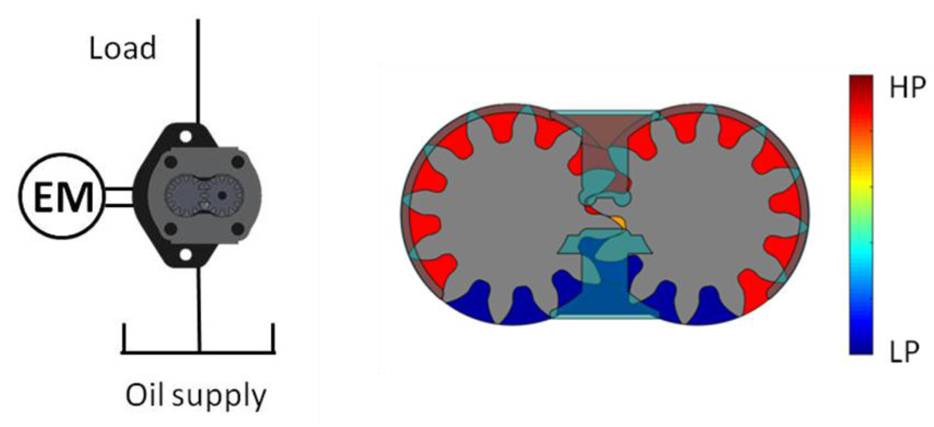
The mechanics of noise generation are very similar between all types of positive displacement machines due to the physics behind the displacing action realized by the machine and the nature of the oscillatory loads acting on the internal parts. A widely used type of displacement machine, the external gear machine (EGM) is taken as a reference for this study with the particular case of the external gear pump (EGP), as shown in Figure 1. The displacing action in an EGM is achieved by the meshing of two gears, which causes the changes of the volume inside every tooth space volume (TSV) in each gear. The fluid is brought into the TSVs on the inlet side; it is then carried around the sides of the gears by the teeth. The displacing action occurs in the meshing zone, where the fluid in the TSV is delivered to the output port, then the new fluid is drawn from the inlet port.
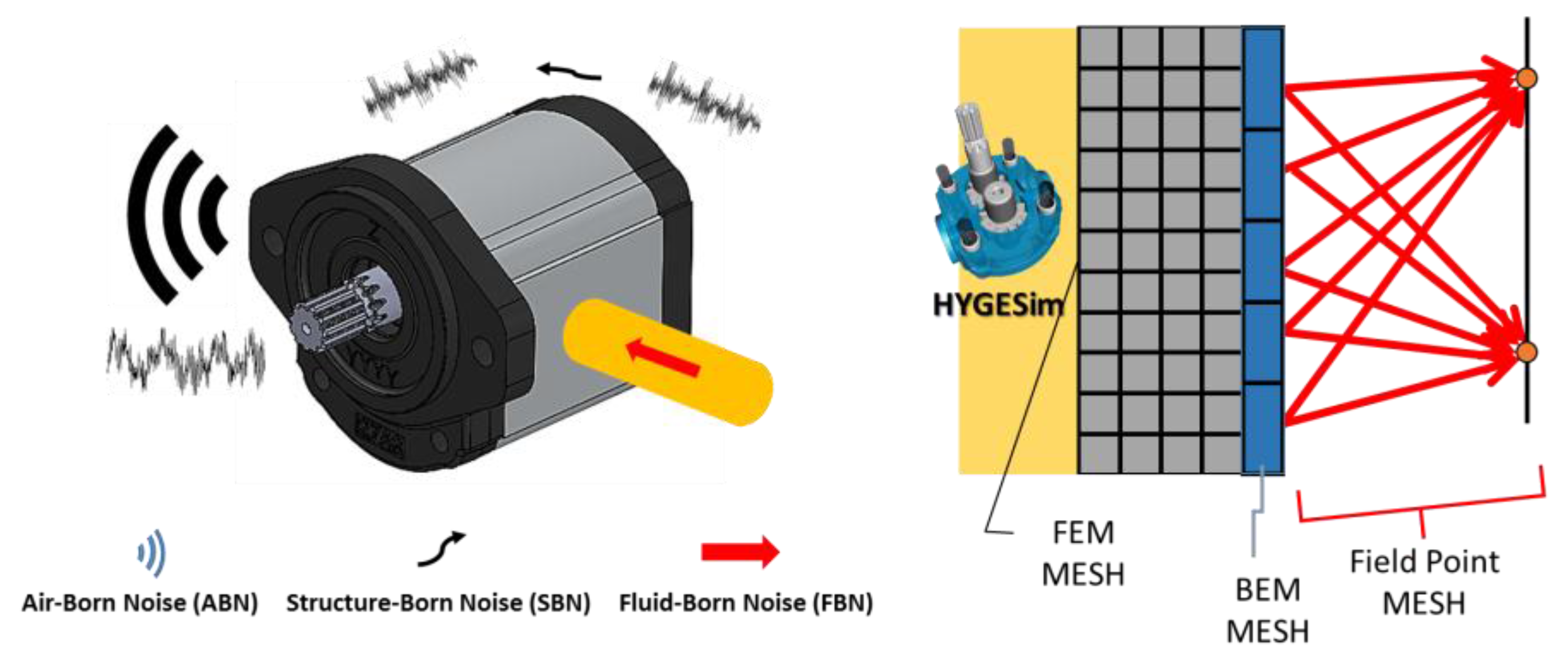
Study of the physical phenomena of noise is typically separated into three categories: fluid, structure, and air-borne noise [1]. The fluid-borne noise (FBN) can be composed of a variety of different phenomena. Primarily, there are large scale pressure fluctuations caused by the displacing action and the resulting loading forces. Additional point sources of noise can be localized cavitation, pressure peaks, and dynamic pressure gradients within the TSVs. As the loads applied by the unit operation interact with the solid body of the pump, the structure-borne noise (SBN) can be separated into two main aspects. The structure is typically considered both as impedance for the transmission of FBN to the environment, and also transmits its own sources of noise in the forms of forces and moments carried by the solid components. Many approaches are available to study the air-borne noise (ABN) for general acoustic applications, while it is difficult to simulate the mechanisms of noise generation in hydrostatic units to predict the fluid-borne noise and structure-borne noise sources.
There have been many studies aimed at reducing the noise in positive displacement machines. While some works focus on reducing internal sources of SBN [2], the main focus in most research on noise in hydraulic pumps is on reducing the magnitude of the pressure ripple oscillations at the outlet port [3,4,5,6,7,8]. For EGMs, this effort has resulted in the formulation of design solutions that involve tooth profile modifications able to reduce the kinematic flow oscillations: Manring and Huang formulated criteria suitable for standard involute designs [6,9]; Negrini introduced the so-called dual-flank principle, a zero-backlash solution currently adopted by several manufacturers that permits to increase the number of displacement chambers [4] to reduce the flow oscillations. Most recent efforts involved the research of non-standard gear profiles—such as asymmetric [10,11], cycloidal-involute [12,13,14,15] able to minimize the kinematic flow oscillations associated with the meshing of the gears. The effects of fluid compressibility on the outlet flow oscillations in EGMs was considered by several researchers, such as Mucchi [5], Casoli et al. [16], Borghi et al. [17], and criteria for minimizing their impact on the flow oscillations through design optimization of recesses facing the gear in the meshing area were provided in several studies, such as [18,19,20]. The source impedance method to characterize FBN through outlet flow oscillations, introduced by Edge et al. [21], was also recently used for EGMs [22]. Despite these efforts, the interaction between pressure ripples and ABN has yet to be clearly investigated [23]. Thus, from the perspective of a quiet pump design, a comprehensive modeling approach is needed in order to investigate the relationship between all the internal sources of FBN including outlet pressure ripples and the SBN and resultant ABN.
In this regard, several authors have addressed different approaches to comprehensively model the acoustic behaviors of EGP. Tang et al. predicted the pump noise based on the combined computational fluid dynamics (CFD) method and the Lighthill’s acoustic analogy (LAA) algorithm, but they only considered the low delivery pressure cases below 3.3 bar [24]. There has been also the numerical-experimental integrated approach that receives the experimentally measured acceleration as an input and calculates the sound field using combined finite element method (FEM) and boundary element method (BEM) [25,26]. Although their approach is simple and useful at the industrial level, preliminary experimental measurements are always required to predict the noise emissions of the pump. A significant contribution was also made by Mucchi et al. who implemented a lumped-parameter model to compute FBN and FEM/BEM model to investigate SBN and ABN [27,28]. Although based on different modeling assumptions particularly related to the determination of the FBN, this latter work is similar to the approach used in this paper. This work also contributes to identifying the different FBN sources and determining their contribution to the overall ABN. This evaluation of FBN noise sources is expected to be useful and effective in seeking the interaction between noise sources and actual noise in the future. Furthermore, in this study, the noise measurements for the model validation were taken inside the semi-anechoic chamber, which can provide more strict and precise determination of sound power levels.
The proposed model takes advantage of a simulation tool for EGM specifically developed by the authors’ research team: HYdraulic GEar machine Simulator (HYGESim) [29]. This simulator provides the accurate dynamic pressure and force information in the fluid (FBN) acting on the pump casing. These predicted noise sources are then classified into four types of load functions (pressures at (1) inlet, (2) outlet, (3) TSV pressure regions, and (4) journal bearing regions) and applied to the corresponding surfaces of the pump structure in a realistic way. After that, the analyses of SBN and ABN are performed by combining a modal analysis performed in ANSYS and an acoustic simulation in LMS Virtual.Lab. Normalized sound power spectra, sound power level (SWL), and sound pressure level (SPL) distributions for the four different operating conditions will be presented as the main outcomes of the acoustic model. The model is validated by showing fairly good agreements with the experimentally measured SWLs. The past work done by the authors’ research team [30] focused on the outlet pressure ripple among all possible noise sources, and partially confirmed the common assumption that outlet pressure ripple is the primary noise source is valid at some shaft speeds. However, the predicted ABN showed a large difference with the measured ABN. The current numerical model is improved by mapping noise sources to the structures in a more realistic way, and the predicted results showed the acceptable difference with the experimental results.
2. Vibro-Acoustic Model of External Gear Pump
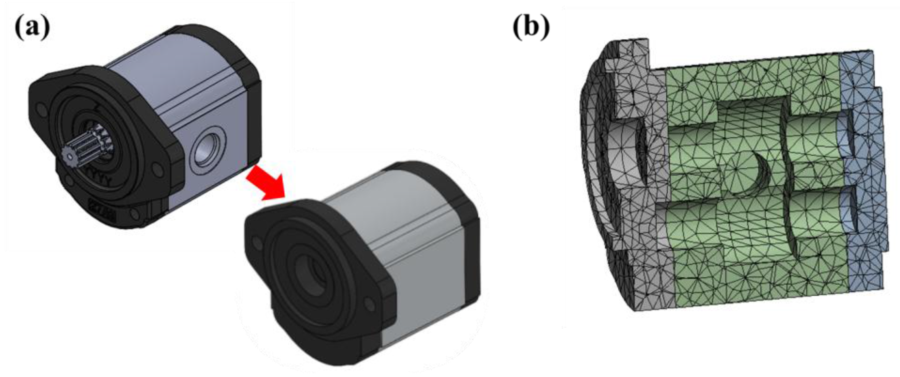
The reference pump considered for this research is a 22 cc/rev commercial no-backlash dual-flank contact gear pump produced by Casappa (model PLP20QW, Parma, Italy). Details of this 12 teeth pump are shown in Figure 2. The pump body is typically composed of three pieces which enclose the gears and have machined ports for connecting the pump to a hydraulic system. The pressure compensated lateral bushings are used for sealing and axial balance. The chosen reference pump is among the most successful designs in mobile hydraulic applications, within pressure ranges up to 300 bar.
2.1. Modeling Approach
The modeling approach follows the three categories of noise generation: fluid-borne noise (FBN), structure-borne noise (SBN), and air-borne noise (ABN), according to the basic idea of the left side of Figure 3. In order to fully model the loading forces (FBN), the structure response (SBN), and the transmission to the air (ABN), a model is needed for each domain.
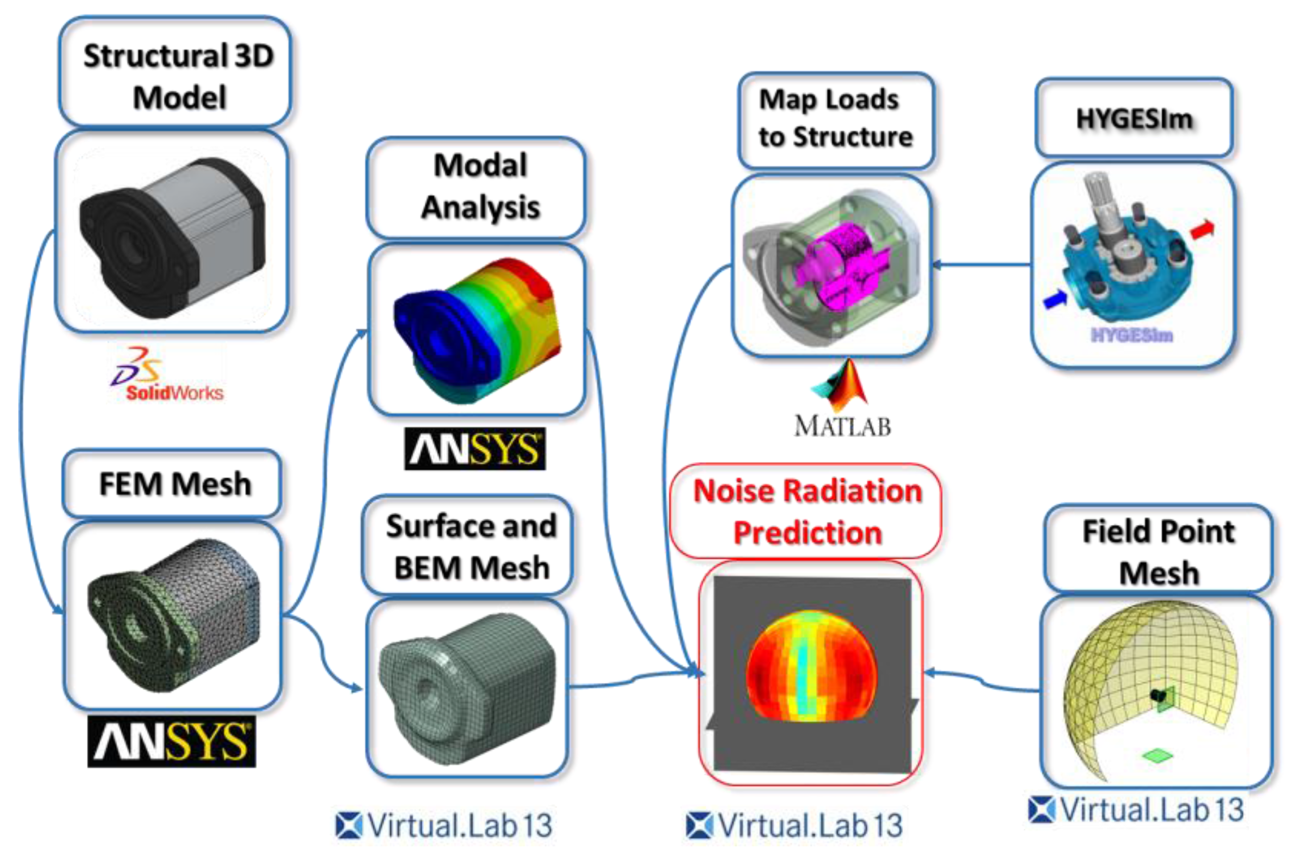
The HYGESim model provides the pressure fluctuations in the fluid (FBN). The predicted dynamic pressure forces in the form of frequency function are used as loading functions to the structure. Then, combined finite element method (FEM) and boundary element method (BEM) approach are used to predict SBN and ABN. The FEM/BEM approach was chosen due to its efficiency and accuracy in predicting the ABN radiated from noise sources; FEM models are widely accepted for the structural vibration, and BEM is accepted as the best for modeling the near-field acoustic effects in models that are placed in unbounded environments. The model type considers the interaction of the load conditions with the mode shapes to investigate the structural vibration of the pump (SBN). Processing the fluid dynamic results involves selecting load and surfaces and mapping loads onto the correct areas of a structural FEM mesh, made in ANSYS. Then, the BEM wrapper mesh technique is used for calculation of the transmission of sound from the pump surface mesh out to the field (ABN). The main structure of the model is adapted from the BEM acoustics methodology for LMS Virtual.Lab Acoustics. A scheme of the sound transmission is represented on the right side of Figure 3, and an overview of the acoustic model is shown in Figure 4. The details of the model will be described in the following sections.
2.2. Model of Internal Fluid-Borne Noise Sources
This section provides a simplified description of the fluid dynamic model of HYGESim, used in this research for the evaluation of the FBN sources.
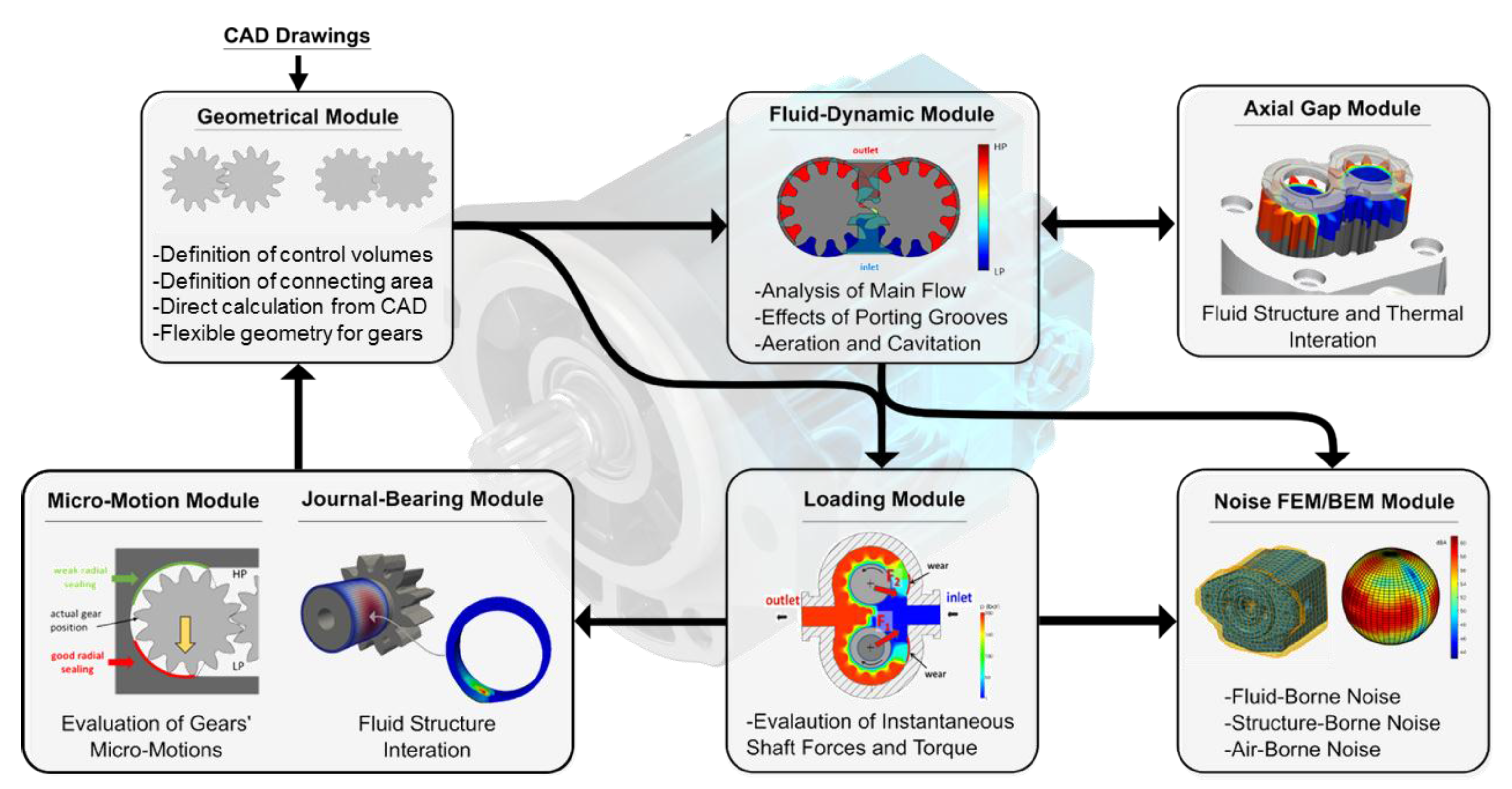
HYGESim is a simulation tool to study for EGMs developed over the last decade at the authors’ research center [31]. As represented in Figure 5, the model can simulate a unit starting from the CAD drawings of the machine. With different modules, HYGESim solves the main flow through the unit considering the radial micro-motions of the gears caused by the pressure forces and contact forces and the behavior of the journal bearings. This is performed through a lumped parameter approach for the solution of the flow displacing action realized by the gears [29], coupled with a numerical solution of the journal bearings [32]. The geometrical model and the control volume schematization, suitable for a large variety of gear profiles, are documented in [33]. For a complete pump simulation, the lubricating gap flow at gear lateral surfaces along that results from the instantaneous position of the floating lateral bushings (Figure 2), a fluid-structure interaction model was developed to run in co-simulation with the solution of the main flow through the EGM [31,34]. Except for the acoustic FEM/BEM module, which will be described in the next sections, all the HYGESim modules are written in C++ language, taking advantage of O-Foam libraries. Only a simplified formulation of the main fluid dynamic model for the analysis of the displacing action is detailed in the following, since it provides the instantaneous pressure used for the loading function of the acoustic simulation of this paper. However, more details on HYGESim can be found in the above-mentioned papers. The acoustic simulation module—represented by the bottom right box in Figure 5—complements the other modules to obtain an omni-comprehensive model capable of predicting the acoustic noise of an EGM.
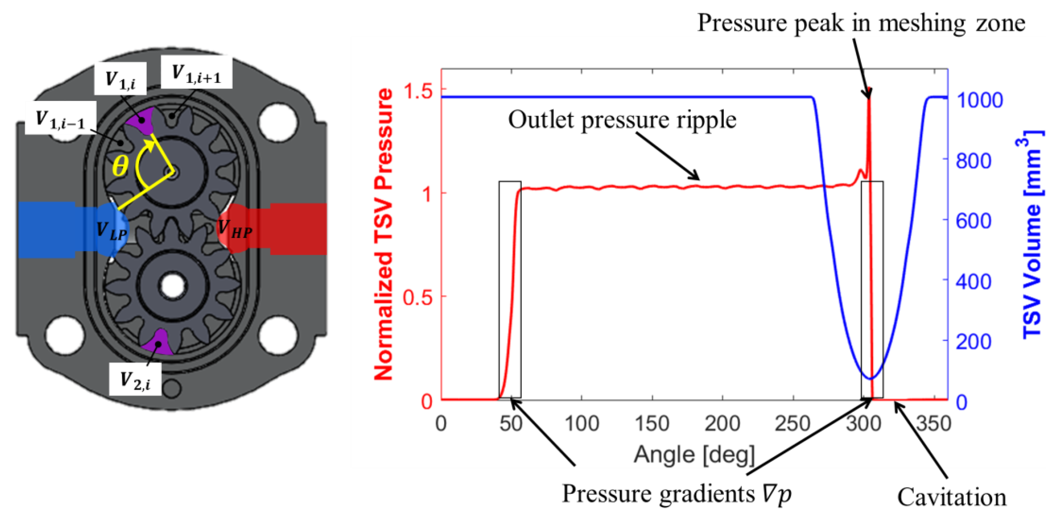
The main fluid dynamic model involves four main control volume groups (as shown in Figure 6). They are the inlet port volume (), the outlet port volume (), the set of control volumes for the TSVs in the drive gear (), and the set of volumes for the TSVs in the slave gear (). The pressure inside the control volumes as a function of fluid properties, geometric volume variation and the net mass transfer with the adjacent control volumes can be given by the pressure build up equation [29]:
where is the pressure, is the time, is the volume, is the variation of the volume with shaft rotation during the meshing process, is the density of the fluid, and and are the mass flow rates entering and leaving the control volume, respectively. In particular, the symbols with the subscript j represent the corresponding quantities inside the j-th control volume. Proper lumped parameter flow equations (orifice flow equation, laminar flow equations for internal leakages) are used to determine the mass flow rate terms entering or leaving each control volume [29].
The fluid dynamic results of HYGESim, in terms of pressures, are used to evaluate the sources of FBN. To better understand how noise sources propagate and what the dominant noise sources are, the key physical phenomena for noise sources need to be understood. As far as the authors are concerned, previous research on acoustic modeling of external gear pump did not clearly define or classify the internal noise sources. Thus, this section describes all possible internal noise sources in the external gear pump that can be observed from the hydrodynamic results of the HYGESim and the noise sources that are concerned in the current acoustic model.
Figure 6 shows the working volume and pressure inside a particular tooth space volume (TSV) calculated by HYGESim, according to the angular convention shown on the left side of the same figure. A single TSV is at full volume for approximately 270° of the gear rotation, and decreases down to minima at the center of the meshing zone. The resulting pressure in that TSV (normalized with the delivery pressure in the order of magnitude of 100 bar) is shown in Figure 6 (red line). A pressure peak results from the compression of the TSV, and its value is mitigated by the internal connections realized in the lateral bushings of Figure 2. This is consistent with what already observed in previous fluid dynamic simulations done by the authors’ team [16,17,29]. Likewise, from 305° through 320°, when the TSV volume increases, the pressure in the TSV falls below atmospheric, causing a little onset of localized aeration [35]. The figure also highlights steep pressure gradients that occur when the TSV pressurizes and decompresses between the high pressure (HP) and low pressure (LP) values respectively at the inlet and at the outlet ports. The TSV pressurization can occur through leakages and/or through proper connections with the outlet port purposely realized on the floating elements, as visible in Figure 7. This latter is the case of the reference unit considered in this work. The whole course of the TSV pressure in Figure 6 is considered as FBN source, applied to a proper region of the casing to be shown in Figure 7.
Another point of noise sources in the figure is given by the outlet pressure fluctuations. It can be noted that for the reference pump the TSV pressure almost coincides with the outlet pressure due to the internal connection to the outlet HP previously mentioned port via the pressurization groove along the edge of the lateral plate (see right side of Figure 7).
Among the mentioned noise sources, the contribution of possible localized cavitation inside the TSV (around 310°) is not considered in the current ABN evaluation, although pressure fluctuations at the inlet port are considered. This simplification reduces implementation complexity, and it is partially justified by the fact that these sources do not directly act on the pump case.
Other noise sources that do not appear in Figure 6, but which are calculated by HYGESim and applied to the structure, are the inlet pressure ripple and the total net radial forces acting on the gears that are carried by the journal bearing regions.
All these noise sources were applied to the structure in order to model the acoustic noise of the EGM. First of all, the basic assumption that all forces must pass through the pump casing in order to radiate out to the surroundings is made. The advantage of this assumption is that if the forces on the interior of the casing separating the interior moving parts from the casing can be accurately modeled, then the moving parts can be removed from the acoustic simulation. Thus, the internal pump components such as the gears are included only in the generation of the loading conditions, but not in the current acoustic propagation model. This simplification also neglects the influence of forces transmitting through the drive gear and coupling into the electric motor or other prime movers.
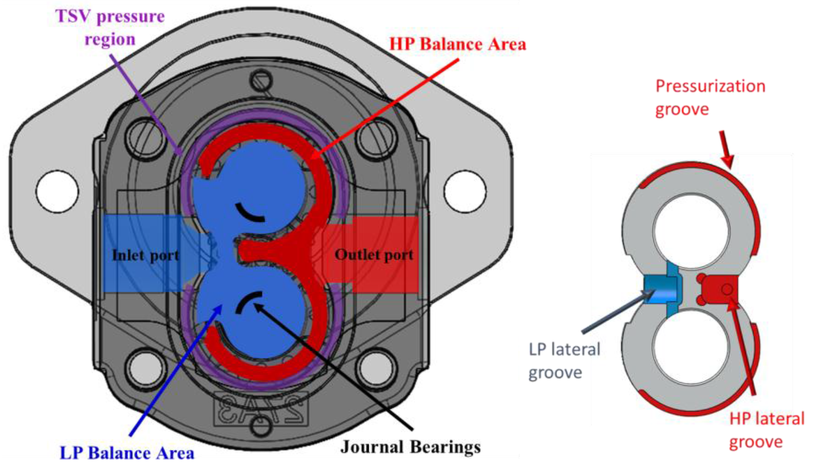
Figure 7 shows the regions exposed to the dynamic pressure in the EGMs, and in this study, these regions are subdivided into 4 areas. First, the case contact with outlet pressure in red occurs at the outlet port and the high-pressure balance area on the lateral bushing. Likewise, the case contact with inlet pressure in blue occurs at the inlet port and the low-pressure balance area on the lateral bushing. In addition, the journal bearing regions in black carry the gear loads. That is, the journal bearing must react all the forces put on the gears by fluid pressures and gear contact forces. Finally, there is a region in purple which is the portion of the case in contact with fluctuating pressure at the whole TSV.
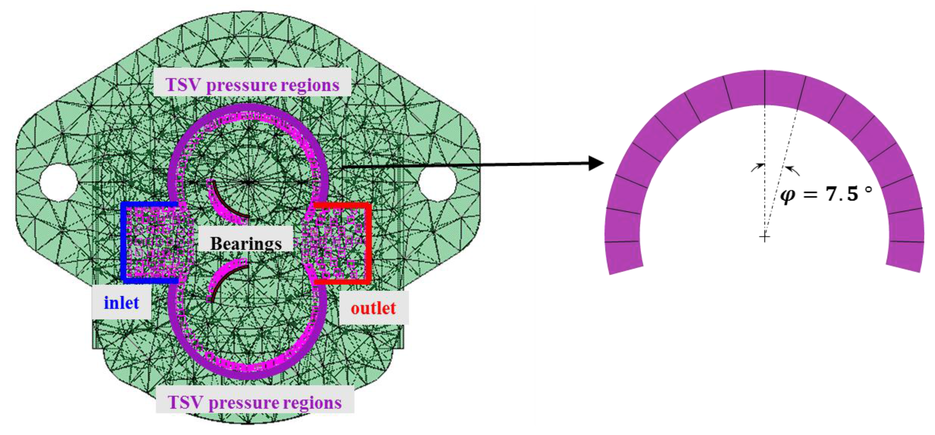
The load area selection on the mesh of the pump geometry corresponding to these areas in the model is shown in Figure 8. All the regions exposed to fluid fluctuations are concerned; the outlet pressure region of the pump is shown in red on the right, the inlet in blue on the left, the TSV pressure regions in a purple arc, and the bearing load areas in black. Specifically, in order to properly map the whole TSV pressure, the circumferential parts of the case are discretized with 7.5 degrees of the angular interval (φ) as shown on the right side of Figure 8. This angular interval was determined based on the sensitivity study which will be discussed in Section 2.5.
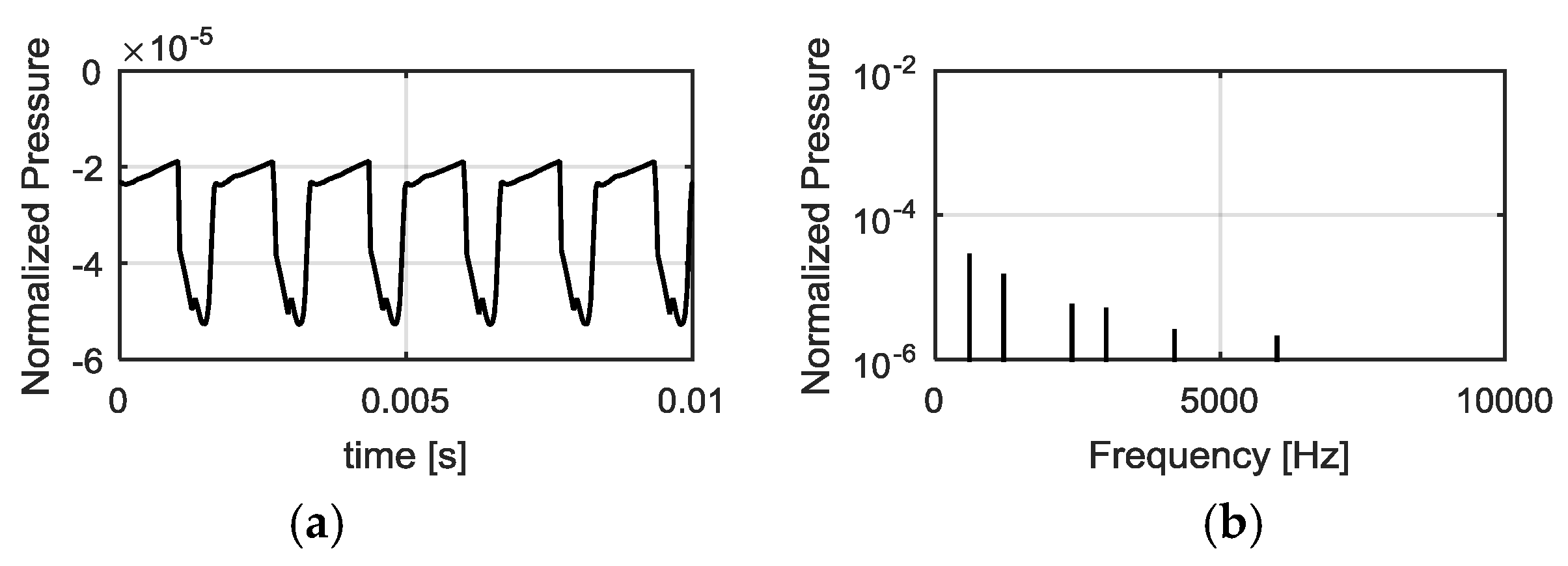
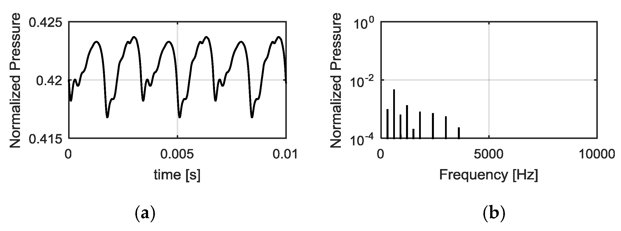
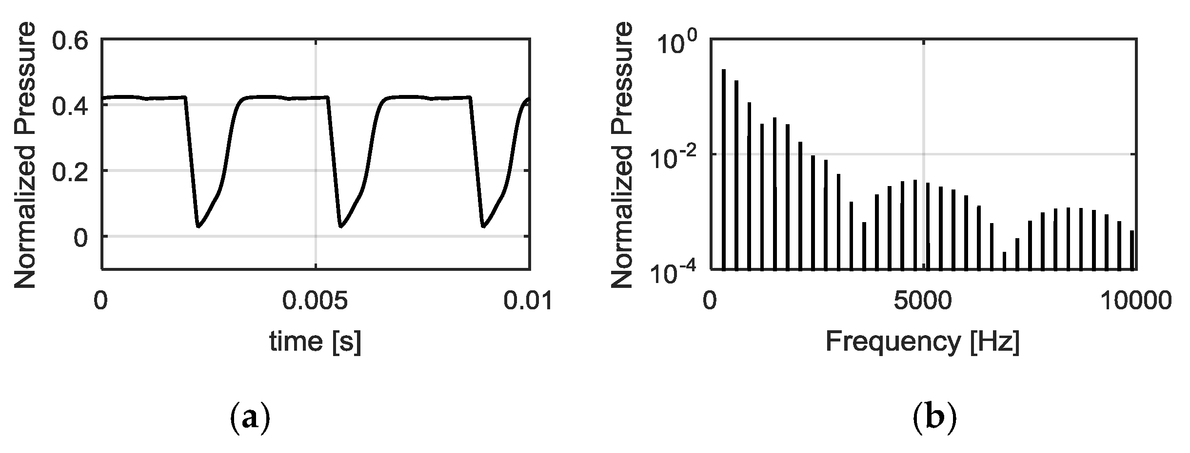
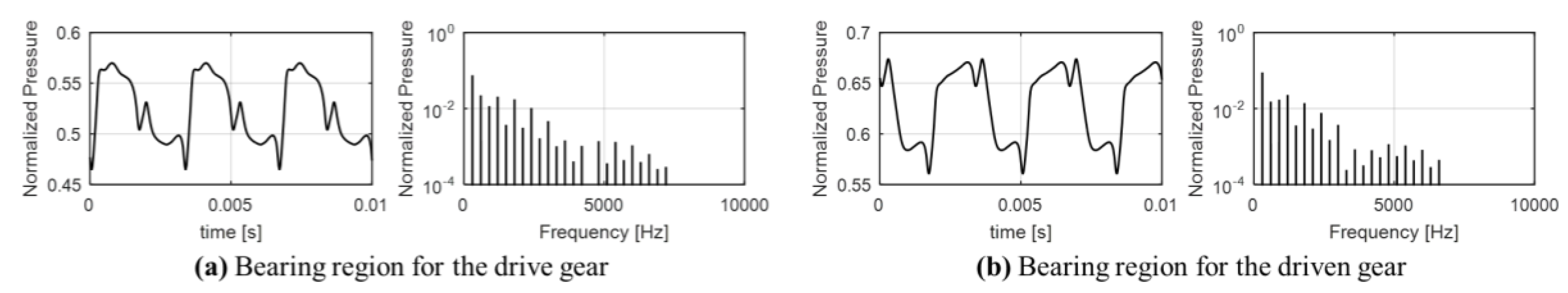
The methodology for load creation is completed in Matlab. The simulated loads that occur at specific surfaces on the model for the operating condition of 1500 rpm shaft speed 100 bar outlet pressure are shown in the following figures (Figure 9: inlet, Figure 10: outlet, Figure 11: TSV pressure regions, and Figure 12: journal bearing regions). The left side of these figures shows the normalized pressure fluctuation depending on time, and the right side of the figures shows Fourier transform of the normalized pressure fluctuation. For brevity, among many discrete points in the TSV pressure regions, only the load on the significant point associated with the pressurization is presented in Figure 11. Note that all the pressure functions in these figures are normalized with the maximum pressure of interest in this study. The loads were applied to the corresponding areas of Figure 8 as functions of frequency. From the figures, it appears that the dynamic pressures acting on the journal bearings and on certain locations of the TSV pressure are larger in magnitude than the outlet pressure ripple, although they are applied to limited area regions. Furthermore, these regions show larger high-frequency components that can be responsible for the high-frequency components of the resultant noise while the outlet pressure ripple seems to only excite the low-frequency noise. This can be supported by the experimental results of a previous research work published by the authors’ team [36]. In this past work, the authors considered only outlet pressure oscillations as FBN source, surface vibrations as SBN, and the radiated airborne noise as ABN. These quantities were measured for shaft speeds ranging from 500 to 2100 rpm, and cross-correlations of FBN-SBN, FBN-ABN, and SBN-ABN were considered. The results showed that there is a very weak correlation between FBN-SBN and FBN-ABN especially at high-frequency regions while the correlation of SBN-ABN is strong through a wide range of frequencies. Thus, both numerical and experimental results imply that the outlet pressure ripple alone can hardly contribute to the high-frequency components of the radiated noise.
2.3. Structural Model of Pump Body Response
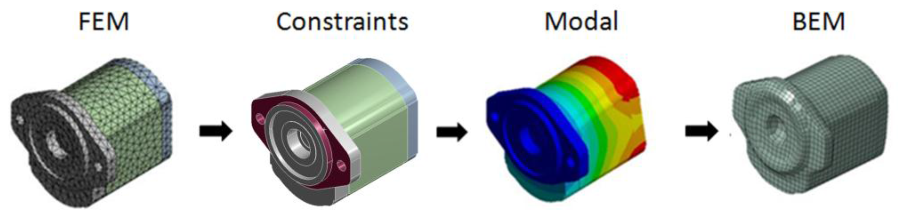
The structural model of the pump is required for determining the potential resonant behavior and the vibrations at the surface of the pumps under operating loads. The modeling approach for predicting SBN is structured in three steps as shown in Figure 13. Starting from the 3 D CAD of the component, the FEM mesh is generated. Next, the modal analysis is performed with a preliminary pump constraining. The final step is the BEM model, with the introduction of a wrapper mesh.
The finite element method (FEM) is a numerical technique for finding approximate solutions to boundary value problems for partial differential equations. The goals for the FEM mesh are to accurately model the modal harmonics and the surface vibration of the pump body. Before generating FEM mesh, the internal pump components such as the gears and shafts were removed because of the assumption that all forces must pass through the pump casing in order to radiate out to the surroundings as described in Section 2.2. Furthermore, the structural model for the reference pump was simplified by eliminating small structural details such as the fillets, grooves, and plaques as shown in Figure 14a. This was done because small structural details have little impacts on the interaction between the low-frequency loading functions and the structure. Furthermore, the quality of FEM mesh can be increased because it prevents the concentration of the nodes and elements near small features on the pump. After the simplification of the pump geometry, the structural meshes were created in ANSYS using a patch-independent tetrahedral mesh as shown in Figure 14b. This mesh allows for the accurate definition of small features while also giving an efficient mesh across large areas. The meshing parameters were determined through the mesh sensitivity study until convergence in the modal frequencies was reached. The detailed information about FEM mesh is given in Table 1. Particularly, the “mapped face meshing” method was applied to the area corresponding to the TSV pressure regions to obtain an even discretization when the meshes were generated.
After that, a modal analysis was performed because it determines the vibration characteristics (natural frequencies and mode shapes) of a structure or a machine component. It can also serve as a starting point for another, more detailed, dynamic analysis, such as a transient dynamic analysis, a harmonic analysis, or a spectrum analysis. The natural frequencies and mode shapes are important parameters in the design of a structure for dynamic loading conditions. Modal frequencies are the frequencies that structural components will react at most strongly if the structure is excited periodically. Mode shapes are the forms the structure will take when it vibrates at a modal frequency. The geometry was tested with constraints, following the real mounting of the pump on a test-rig or commercial/industrial application as shown in the middle of Figure 13: the holes on the flange and the mounting area are fixed and the structures are bounded along the axial direction. The natural frequencies (normalized with respect to the first mode) are shown in Table 2. All these 16 modes are in the audible frequency range and considered in the acoustic model.
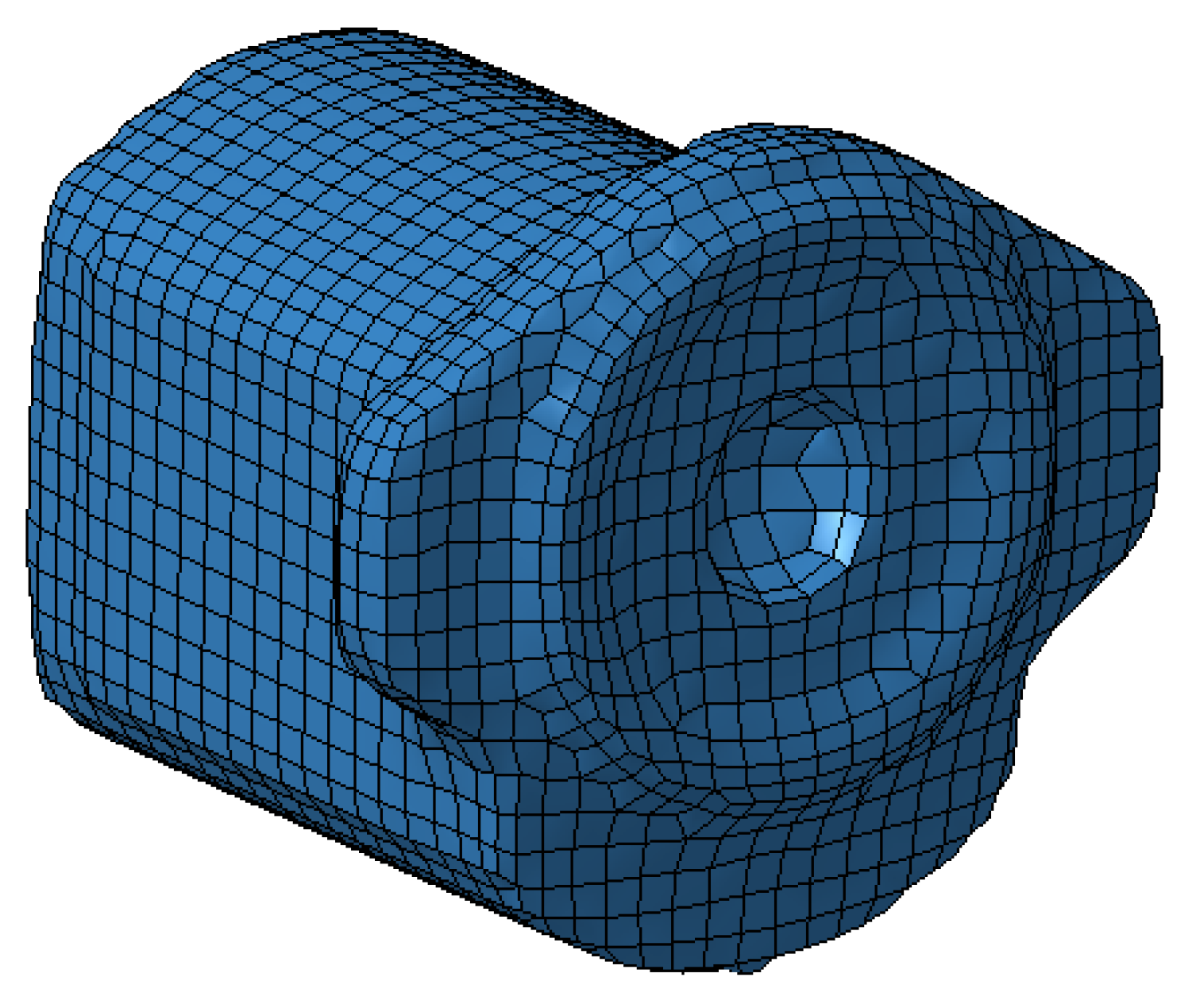
The final step to the structural model is to generate the boundary element surface mesh made in LMS Virtual.Lab Acoustics as shown in Figure 15. The BEM mesh size was chosen to 5 mm maximum element size in order to achieve a material maximum frequency up to 10 kHz (the maximum element size was determined to satisfy that the number of elements per the shortest wavelength is 6). The size of the boundary elements is regularly distributed across the whole mesh. The number of quadrilateral elements and nodes of BEM mesh were 2453 and 2451 respectively.
2.4. Acoustic Model
The next step for predicting the acoustic noise of the pumps is to model the acoustic environment for the exterior domain. To do this, the field point mesh (FPM) and two reflecting planes were introduced as shown in Figure 16 in order to mimic the environments of the semi-anechoic chamber where noise measurements were conducted for the model validation (as it will be seen in Section 3.2). Two reflecting planes represent the floor and wall inside the sound chamber. Because the floor and wall are assumed to be rigid, the so-called image method is used in the software; two symmetry planes generate the mirror images of noise sources against the planes and the boundaries are removed, which are acoustically equivalent to the presence of the rigid planes. This method can make the problems simpler and allow more efficient computation. In addition, the FPM is a visualization mesh, which is used to compute and represent the acoustic results in space around the vibrating pumps. This mesh does not influence the acoustical solution but simply limits the number of environmental solution points (each point of FPM can be regarded as the microphone). To get the mesh geometry in Figure 16, a spherical mesh of 1-meter radius from the center of the pump was first generated and then, mesh elements located below the floor and behind the wall were removed.
After creating FPM and reflecting planes, a modal superposition vibro-acoustic response simulation type is run in LMS Virtual.Lab. This type sets up and solves the coupled FEM/BEM equation involving both the structural displacements () and the acoustic pressure (: pressure at the nodes of coupling interface, : pressure at the remaining nodes) as unknowns:
where is the stiffness matrix, is the damping matrix, is the mass matrix, is the coupling matrix, is the transformation matrix that relates the normal velocity to the displacement, and are the matrices that relate nodal pressure values to the nodal normal velocity, and are the vectors that contain the prescribed structural and acoustical the boundary conditions set, is the angular frequency, and is the density of the air. The details of the equations put into practice in the model can be found in the works done by Desmet et al. [37]. This model form allows to compute the response of the system using a modal model and a given load data set. This case assumes the modal damping matrix to be purely diagonal, and does not make an actual projection of the system of equations onto the modal basis.
2.5. Sensitivity Study on the Angular Interval for Discretization of the TSV Pressure Region
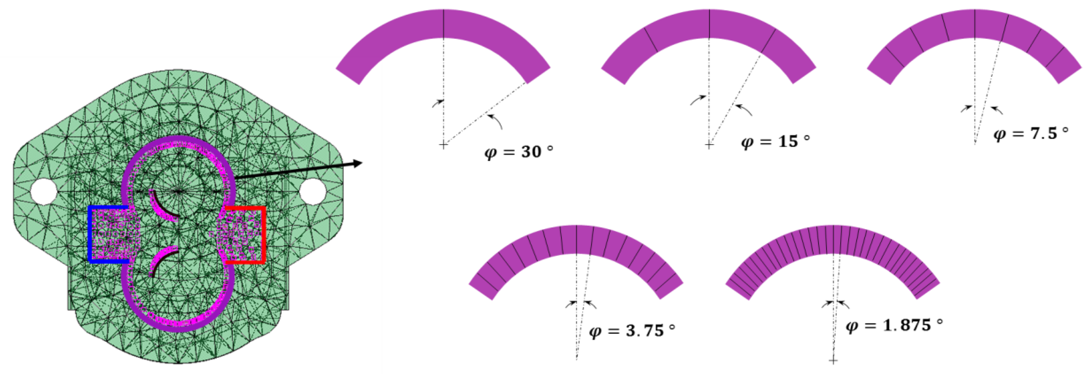
In this work, the area of the EGM case next to the TSV pressure region (Figure 7) was discretized to properly map the pressure of the moving TSV to the stationary pump case. If this region is not divided into enough number of sections, high spatial discontinuity of the loads brings the acoustic model far from realistic. While the larger number of split sections in the TSV pressure region enables the gentler and more realistic spatial variation of the loads, it increases computing time and efforts. Thus, a sensitivity study was performed to determine the reasonable angular interval for discretization of the TSV pressure region. (Smaller angular interval means larger number of split sections in the TSV pressure region).
Figure 17 shows the overview of the sensitivity study cases. First, the angular interval of a TSV (30°, for a 12 teeth unit) was chosen as the largest angular interval for discretization of the TSV pressure region. Then, finer angular intervals were considered by progressively reducing by half, until it reached 1.875 degree. Consequently, 5 cases were considered with the following angular intervals: 30, 15, 7.5, 3.75, and 1.875 degrees, which means that the numbers of split sections in one TSV angle are 1, 2, 4, 8, and 16. Then, the acoustic results of 5 cases for the operating condition of 1500 rpm shaft speed and 100 bar outlet pressure were compared.
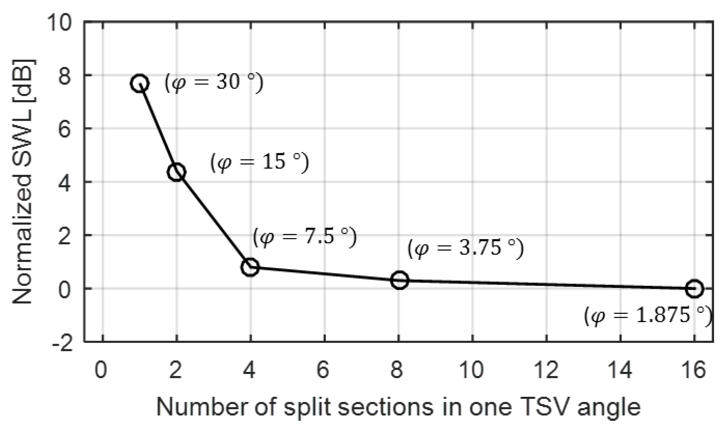
Figure 18 shows the normalized SWLs for the five considered cases (the reference was set to the SWL for the case of 1.875 degree of the angular interval). The figure shows how the simulated SWL decreases as the number of sections in the TSV pressure region is increased. The spatially gentle variation of the loads in this region caused by increasing the number seems to bring lower SWL. More notable is the amount of change in SWL over the number of split sections. While SWL greatly decreases as the number of split sections in one TSV angle increases up to 4, the SWL variations become almost negligible (less than 1 dB) as the number is larger than 4. This leads to the conclusion that 7.5° (corresponding angle to 4 split sections in one TSV angle) is small enough for the angular interval for discretization of TSV pressure region.
3. Acoustic Results
3.1. Numerical Results
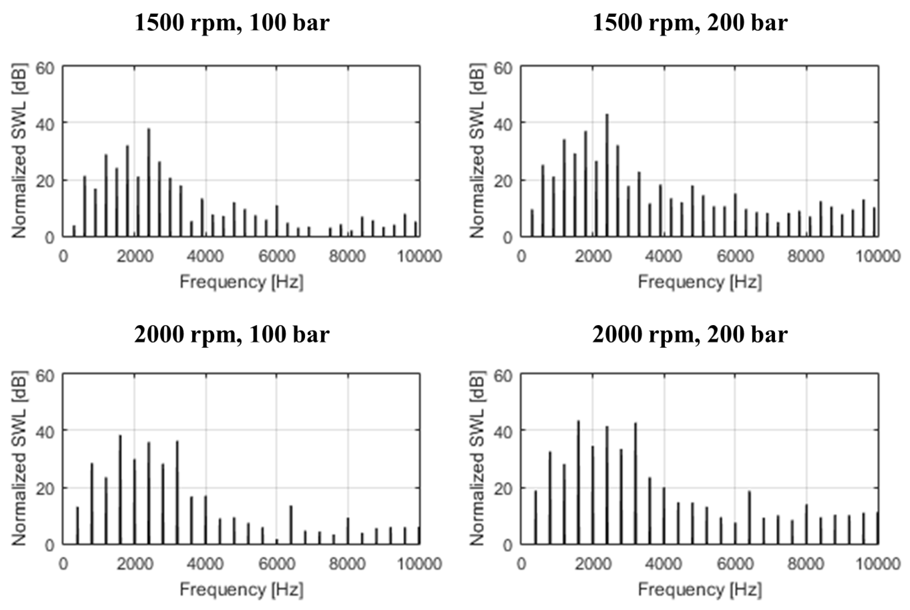
SWL and SPL are considered for four different operating conditions as the main output of the acoustic model. These were calculated every 15 Hz (for 1500 rpm shaft speed) and 20 Hz (for 2000 rpm shaft speed) between 0 and 10 kHz.
The resulting normalized sound power spectra are shown in Figure 19. Note that the normalized SWL was referenced to the sound power of the experimentally measured mean noise floor inside the semi-anechoic chamber (experimental measurements for validation were taken as will be described in Section 3.2). It means that the noise level corresponding to the measured mean noise floor was designated as 0 dB. Because coupling with the electric motor or other prime mover was not considered in the model, harmonics of the shaft rotational frequency (fundamentals of 1500 and 2000 rpm are 25 and 33.3 Hz, respectively) are not effective. Taking into account that the number of gear teeth is 12 and so the fundamentals of meshing frequency are 300 and 400 Hz, harmonics of the meshing frequency are dominant in the sound power spectra. The fundamental of meshing frequency () was calculated by Equation (3):
where is the number of gear teeth and is the shaft speed in rpm. Another observation one can make is that the noise level at the second harmonic is higher than the level at the first harmonic. This can be explained by the zero backlash (dual flank) nature of the displacing action of the considered EGM.
By integrating each frequency component, it is possible to obtain a value identifying the overall sound power level. Table 3 shows the normalized overall sound power levels for the four operating conditions. Note that the overall SWLs were also referenced to the same value used for the calculation of sound power spectra in Figure 19.
Increasing the outlet pressure from 100 to 200 bar at the shaft speed of 1500 rpm, the SWL rises by 5.1 dB. Keeping the same outlet pressure of 100 bar, and increasing the shaft speed to 2000 rpm results in 2.6 dB increase in the noise level. Finally, increasing shaft speed and outlet pressure at the same time, the SWL enhances by 8.1 dB compared to the initial condition of 1500 rpm, 200 bar.
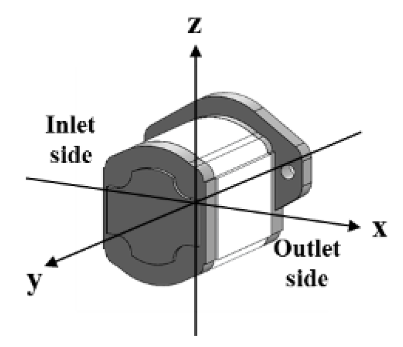
Next, consider the SPL distribution. Figure 20 shows the coordinate system for the SPL distribution. Positive and negative x directions represent the inlet and outlet side, respectively. The back side and the flange side are set to the positive and negative y directions.
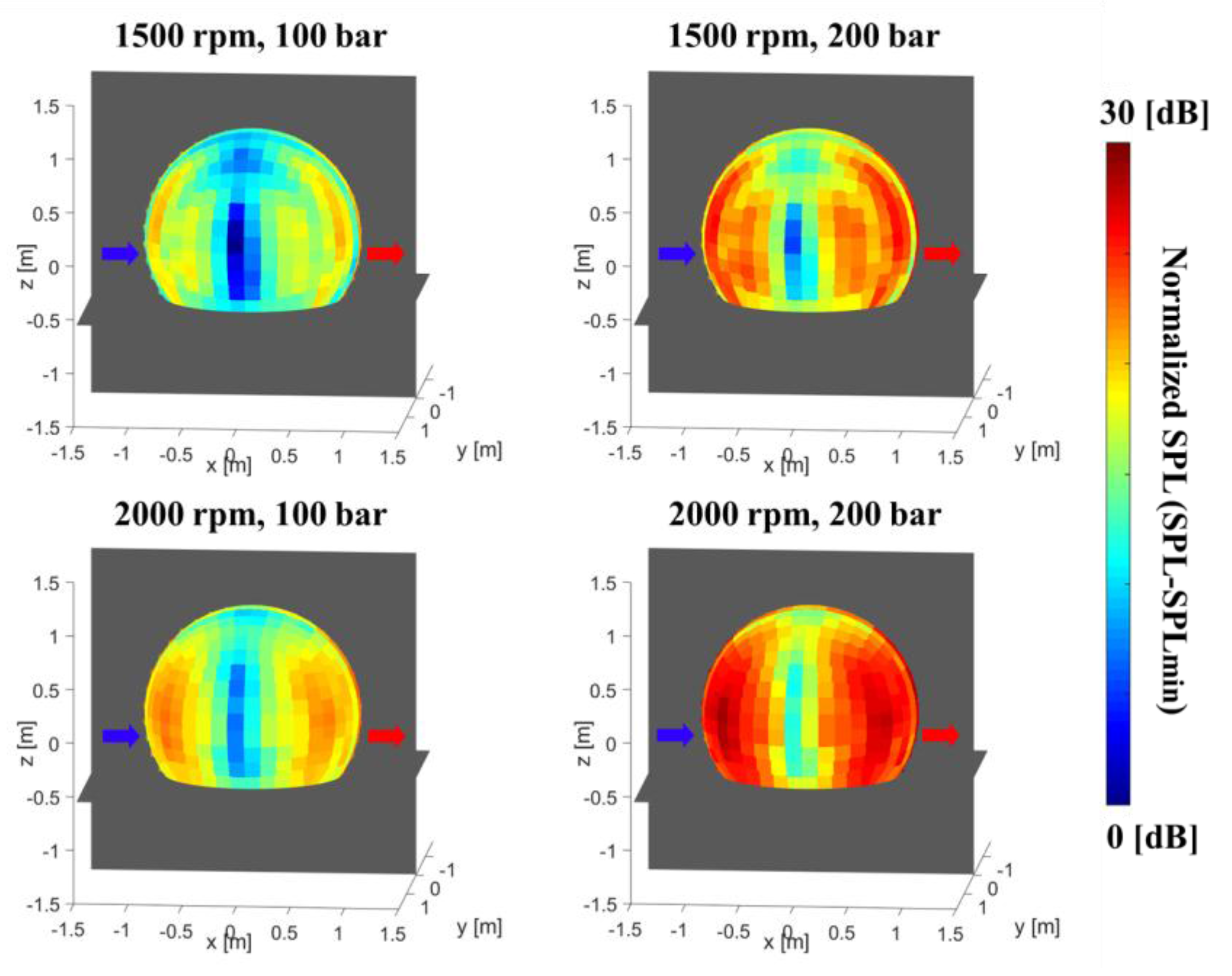
Figure 21 shows the SPL distribution at the distance of 1 m from the pump for 4 different operating conditions. The pump is located at the origin. The blue arrow indicates the inlet side of the pump while the red arrow indicates the outlet side. Two reflecting planes for the wall and floor are represented in gray. Note that SPLs are normalized with the global minimum SPL of the entire results. In each case, there are crucial red areas on the inlet and outlet sides (positive and negative x-direction). Furthermore, the effect of increasing speed shaft and outlet pressure is quite similar, as confirmed from the analysis of SWL; changing both the shaft speed and outlet pressure, it is possible to observe an increase and an enlargement of the dark red zone on the mesh.
3.2. Experimental Validation
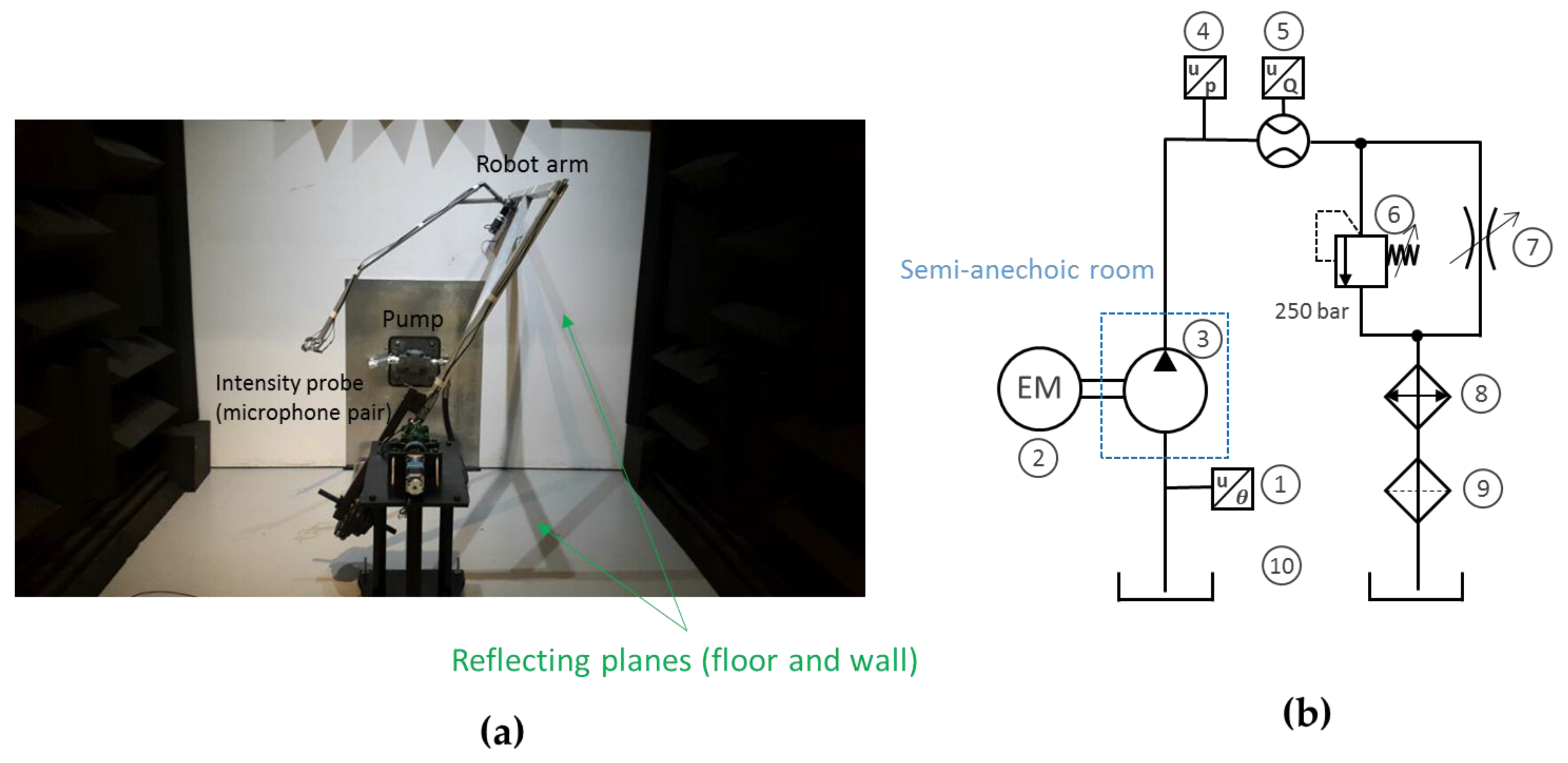
To validate the presented acoustic model, experimental noise measurements were taken using the semi-anechoic chamber available at the Maha Fluid Power Research Center of Purdue University as shown in Figure 22a. The open hydraulic circuit used for the experiments is shown in Figure 22b, with further details reported in Table 4. The pump under testing and short connecting lines were inside of the sound chamber, while the driving electric motor and other hydraulic components were isolated behind reflecting walls. The measurement procedure used for the tests can be summarized as follows. The electric motor was started at the desired shaft speed and the variable orifice at the pump outlet is gradually closed until the desired outlet pressure was reached. After that, the cooling circuit was adjusted to maintain the inlet temperature constant at 50 °C (under an accuracy of 1 °C). Then, noise measurements were taken as soon as steady state conditions of inlet temperature were achieved.
The sound power levels of pump noise at 4 different operating conditions were determined closely following ISO 9614-1: 1993 [38]. The measurement surface was chosen the same with the geometry of field point mesh in Figure 16, which was the remaining parts of the sphere of 1-meter radius from the pump excluding the areas behind the wall and below the floor. The measurement points were evenly distributed by the number of 107 over the surface enclosing the sound source. The number of 107 points was determined by the grid study with a different number of measurement points, which showed the reasonable accuracy and measuring time.
The sound intensities at discrete points were measured over the selected surface. Theoretically, it is ideal for the sound intensity to be measured at multiple points at the same time using multiple intensity probes. Due to the cost constraint, however, one sound intensity probe composed of three microphones (GRAS, three microphones Type 40A0—Sensitivity 0.2 dB ref 20 , ½“ diameter) was moved to the corresponding measurement points using the robot arm under the assumption that the noise emission remains unchanged during the steady-state operating condition. The sound intensity was calculated based on the cross-spectral density of the sound pressure signals measured at two microphones using the following equation:
where is the sound intensity in r direction, is the density of air, is the angular frequency of interest, is the distance between two microphones, and is the cross-spectral density of sound pressures measured at microphone 1 () and 2 (). The details of sound intensity calculation can be found in [39]. Lastly, sound power was obtained by integrating the measured sound intensity over the measurement surface.
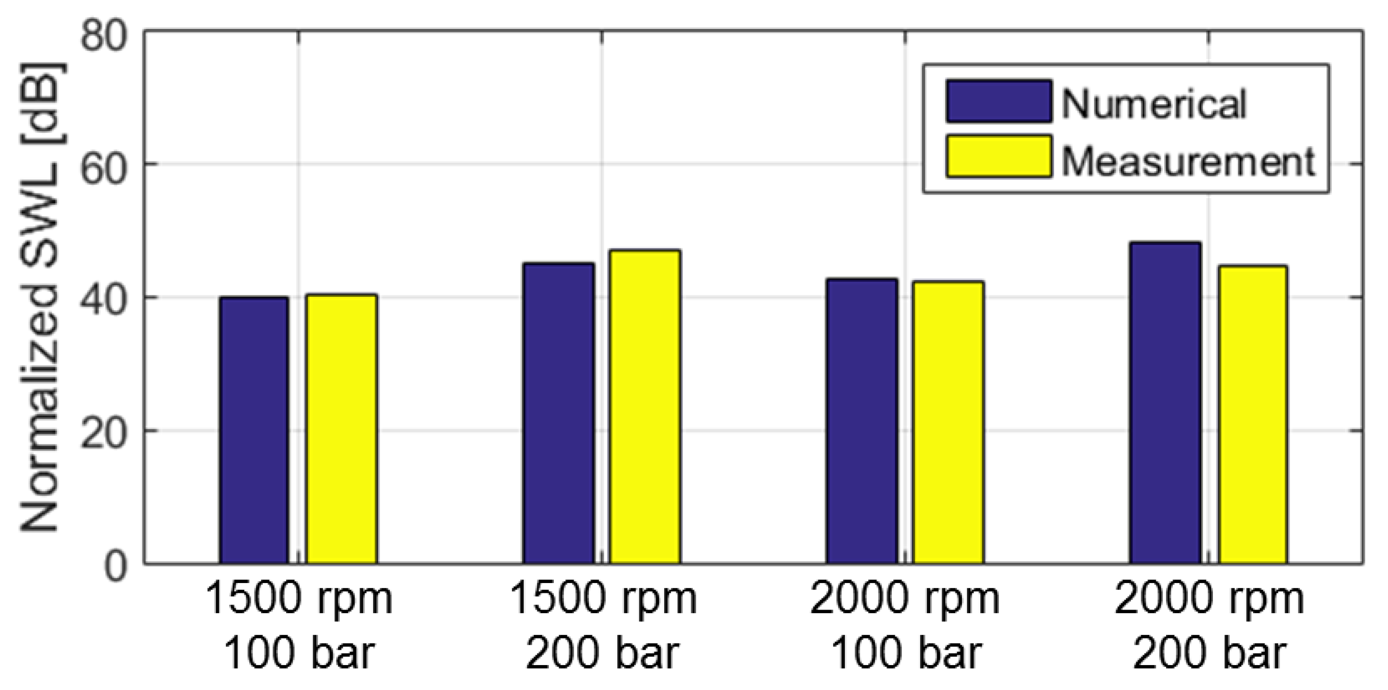
The normalized overall SWLs of experimental results for 4 different operating conditions obtained by the procedure mentioned above were compared with the numerical results as shown in Figure 23 and Table 5. Note that the reference of SWL is the same value used in Section 3.1. Similar trends of numerical results can be seen in the experimental results; as the delivery pressure and the shaft speed are increased, overall SWL tends to be increased. However, this trend is found not to be always true. In the experiments, SWL for the operating conditions of 1500 rpm 200 bar showed the higher value than 2000 rpm 200 bar. This may be because resonant behaviors of the pump and attached structures can be changed by different shaft speeds as the shaft speed determines the system excitation frequency. Furthermore, it can be seen that numerical and experimental results are very close to each other within the acceptable ranges of noise level differences; while the noise level difference of 3.4 dB for 2000 rpm, 200 bar is a little high, the difference for other 3 operating conditions are less than 2 dB. This result can support the validity of our acoustic model.
In terms of SPL distributions, trends similar to the numerical results of Figure 21 were observed in the experimental results. In particular, noisy areas are present near the inlet and outlet sides. Furthermore, an increase of the delivery pressure does not greatly change the overall shapes of the SPL distributions, but it results in an increment of the overall noise level. However, the agreement between the experimental and numerical results that pertains to the SPL distributions is not as close as the one related to the SWL comparison. There are multiple reasons for a possible mismatch related to the experimental environment. For instance, the coupling with the electric motor, the presence of the robot, and the properties of the walls in the anechoic room were neglected or approximated by the model. However, the main discrepancies between numerical and experimental results seem to come from the absence of the structures attached to the pump in the acoustic model. While the standalone pump was considered in the acoustic model, the actual noise can come from the vibration of structures attached to the pump such as lines and plates as well as the vibrations of the pump itself. Including the attached structures can change the resonant behavior of the whole system. Thus, by further developing the current acoustic model, the effects of different mounting situations on noise emissions can be studied in the future. These considerations will also allow for a better accuracy of the results pertaining the SPL distributions representative of noise directionality. However, the current model can predict the “total” sound energy radiated by the pump per unit time (overall SWL) with a fairly good accuracy. Thus, the current acoustic model shows the potentials to investigate the dominant noise sources in a deeper level and serve for future studies aimed at designing quieter pumps.
4. Conclusions
This paper presented a numerical model for the evaluation of the noise emitted by EGMs along with its experimental validation. The sources of fluid-borne noise (FBN) were evaluated taking advantage of the results provided by the authors’ HYGESim (HYdraulic GEar machine Simulator) model. In particular, a procedure to evaluate the dynamic pressure forces acting on the pump case was defined for the outlet pressure region, the inlet pressure region, the tooth space volume (TSV) pressure region and the region of the journal bearings. Vibration and sound radiation were then predicted using a combined finite element and boundary element vibro-acoustic model.
Considering a commercial pump as reference unit, normalized sound power spectra, sound power level (SWL), and the sound pressure level (SPL) distributions for the different operating conditions were discussed. The results showed the general trends that both SWL and SPL increase with both the shaft speed and the outlet pressure.
An experimental activity was performed using a semi-anechoic room at the Maha Fluid Power Research Center, and the numerical results were compared with the experimentally measured SWL to validate the acoustic model. The numerically predicted SWL showed similar values than the experimental results conducted in the semi-anechoic chamber.
The proposed model shows how an accurate prediction of the noise emitted by an EGM is possible with a good accuracy on the base on an acoustic model that considers all the most important FBM noise sources. In future, the presented model can serve studies related to the design of quieter EGMs. For this purpose, it is worthwhile to observe that alternative simulation packages could be used to implement a similar simulation workflow for the analysis of FBN, SBN and ABN. Additionally, the authors believe that the software interfacing presented in this work might also be useful to advance the development of commercial software towards the simulation of noise emissions in positive displacement machines.
Acknowledgments
The authors would like to express their gratitude to Siemens for the use of AMESim and LMS Virtual.Lab.
Author Contributions
Sangbeom Woo, Timothy Opperwall, and Andrea Vacca conceived the simulation model, designed and performed the validation experiments performed at the Maha Fluid Power Research Center of Purdue University. Manuel Rigosi provided all technical data of the reference pump, and he also provided technical assistance in all activities of the project. All the authors analyzed the data and wrote the paper.
Conflicts of Interest
The authors declare no conflict of interest.
References
- Fiebig, W. Location of noise sources in fluid power machines. Int. J. Occup. Saf. Ergon. 2007, 13, 441–450. [Google Scholar] [CrossRef] [PubMed]
- Bonanno, A.; Pedrielli, F. A study of the structure borne noise of hydraulic gear pumps. In Proceedings of the 7th JFPS International Symposium on Fluid Power, Toyama, Japan, 15–18 September 2008; pp. 641–646. [Google Scholar]
- Edge, K.A. Designing quieter hydraulic systems—Some recent developments and contributions. In Proceedings of the Fourth JHPS International Symposium on Fluid Power, Tokyo, Japan, 15–17 November 1999; pp. 3–27. [Google Scholar]
- Negrini, S. A gear pump designed for noise abatement and flow ripple reduction. In Proceedings of the International Fluid Power Exposition and Technical Conference, Chicago, IL, USA, 23–25 April 1996. [Google Scholar]
- Mucchi, E.; Dalpiaz, G.; Del Rincon, A.F. Elastodynamic analysis of a gear pump. Part I: Pressure distribution and gear eccentricity. Mech. Syst. Signal Proc. 2010, 24, 2160–2179. [Google Scholar] [CrossRef]
- Manring, N.D.; Kasaragadda, S.B. The theoretical flow ripple of an external gear pump. ASME J. Dyn. Syst. Meas. Control 2003, 125, 396–404. [Google Scholar] [CrossRef]
- Harrison, K.A.; Edge, K.A. Reduction of axial piston pump pressure ripple. Proc. Inst. Mech. Eng. Part I J. Syst. Control Eng. 2000, 214, 53–64. [Google Scholar] [CrossRef]
- Opperwall, T.; Vacca, A. Modeling noise sources and propagation in displacement machines and hydraulic lines. In Proceedings of the 9th JFPS International Symposium on Fluid Power, Matsue, Japan, 28–31 October 2014. [Google Scholar]
- Huang, K.J.; Chen, C.C. Kinematic displacement optimization of external helical gear pumps. Chung Hua J. Sci. Eng. 2008, 6, 23–28. [Google Scholar]
- Morselli, M.A. Geared Hydraulic Machine and Relative Gear Wheel. U.S. Patent 20150330387 A1, 19 November 2015. [Google Scholar]
- Devendran, R.S.; Vacca, A. Design potentials of external gear machines with asymmetric tooth profile. In Proceedings of the ASME/Bath Symposium on FPMC 2013, Sarasota, FL, USA, 8–11 October 2013; p. 12. [Google Scholar]
- Nagamura, K.; Ikejo, K.; Tutulan, F.G. Design and performance of gear pumps with a non-involute tooth profile. Proc. Inst. Mech. Eng. Part B J. Eng. Manuf. 2004, 218, 699–711. [Google Scholar] [CrossRef]
- Zhou, Y.; Hao, S.; Hao, M. Design and performance analysis of a circular-arc gear pump operating at high pressure and high speed. Proc. Inst. Mech. Eng. Part C J. Mech. Eng. Sci. 2016, 230, 189–205. [Google Scholar] [CrossRef]
- Morselli, M.A. A Positive-Displacement Rotary Pump with Helical Rotors. EP Patent 1132618 B1, 30 April 2008. [Google Scholar]
- Lätzel, M.; Schwuchow, D. An innovative external gear pump for low noise applications. In Proceedings of the 8th International Fluid Power Conference (IFK), Dresden, Germany, 26–28 March 2012. [Google Scholar]
- Casoli, P.; Vacca, A.; Franzoni, G.; Guidetti, M. Effects of some relevant design parameters on external gear pumps operating: Numerical predictions and experimental investigations. In Proceedings of the 6IFK Internationales Fluidtechnisches Kolloquium, Dreden, Germany, 31 March–2 April 2008. [Google Scholar]
- Borghi, M.; Milani, M.; Zardin, B.; Patrinieri, F. The influence of cavitation and aeration on gear pump and motors meshing volume pressures. In Proceedings of the ASME International Mechanical Engineering Congress & Exposition, Chicago, IL, USA, 5–10 November 2006; pp. 47–56. [Google Scholar]
- Wang, S.; Sakurai, H.; Kasarekar, A. The optimal design in external gear pumps and motors. IEEE/ASME Trans. Mechatron. 2011, 16, 945–952. [Google Scholar] [CrossRef]
- Mucchi, E.; Tosi, G.; D’Ippolito, R.; Dalpiaz, G. A robust design optimization methodology for external gear pumps. In Proceedings of the ASME 2010 10th Biennial Conference on Engineering Systems Design and Analysis ESDA 2010, Istanbul, Turkey, 12–14 July 2010; pp. 1–10. [Google Scholar]
- Devendran, R.S.; Vacca, A. Optimal design of gear pumps for exhaust gas aftertreatment applications. Simul. Model. Pract. Theory 2013, 38, 1–19. [Google Scholar] [CrossRef]
- Edge, K.A.; Johnston, D.N. The “secondary source” method for the measurement of pump pressure ripple characteristics Part 1: Description of method. Proc. Inst. Mech. Eng. Part A J. Power Energy 1990, 204, 33–40. [Google Scholar] [CrossRef]
- Nakagawa, S.; Ichiyanagi, T.; Nishiumi, T. Experimental investigation on effective bulk modulus and effective volume in an external gear pump. In Proceedings of the BATH/ASME 2016 Symposium on Fluid Power and Motion Control, Bath, UK, 7–9 September 2016. [Google Scholar]
- Hartmann, K.; Harms, H.H.; Lang, T. A model based approach to optimize the noise harmonics of internal gear pumps by reducing the pressure pulsation. In Proceedings of the 8th International Fluid Power Conference (IFK) 2012, Dresden, Germany, 26–28 March 2012. [Google Scholar]
- Tang, C.; Wang, Y.S.; Gao, J.H.; Guo, H. Fluid-sound coupling simulation and experimental validation for noise characteristics of a variable displacement external gear pump. Noise Control Eng. J. 2014, 62, 123–131. [Google Scholar] [CrossRef]
- Carletti, E.; Miccoli, G.; Pedrielli, F.; Parise, G. Vibroacoustic measurements and simulations applied to external gear pumps: An integrated simplified approach. Arch. Acoust. 2016, 41, 285–296. [Google Scholar] [CrossRef]
- Miccoli, G.; Carletti, E.; Pedrielli, F.; Parise, G. Simplified methodology for pump acoustic field analysis: The effect of different excitation boundary conditions. In Proceedings of the Inter-Noise 2016, Hamburg, Germany, 27–30 August 2016; pp. 3984–3992. [Google Scholar]
- Mucchi, E.; Dalpiaz, G. Numerical vibro-acoustic analysis of gear pumps for automotive applications. In Proceedings of the International Conference on Noise and Vibration Engineering ISMA 2012, Leuven, Belgium, 17–19 September 2012; pp. 3951–3961. [Google Scholar]
- Mucchi, E.; Rivola, A.; Dalpiaz, G. Modelling dynamic behaviour and noise generation in gear pumps: Procedure and validation. Appl. Acoust. 2014, 77, 99–111. [Google Scholar] [CrossRef]
- Vacca, A.; Guidetti, M. Modelling and experimental validation of external spur gear machines for fluid power applications. Simul. Model. Pract. Theory 2011, 19, 2007–2031. [Google Scholar] [CrossRef]
- Opperwall, T.; Vacca, A. A combined FEM/BEM model and experimental investigation into the effects of fluid-borne noise sources on the air-borne noise generated by hydraulic pumps and motors. Proc. Inst. Mech. Eng. Part C J. Mech. Eng. Sci. 2014, 228, 457–471. [Google Scholar] [CrossRef]
- Dhar, S.; Vacca, A. A fluid structure interaction-EHD model of the lubricating gaps in external gear machines: Formulation and validation. Tribol. Int. 2013, 62, 78–90. [Google Scholar] [CrossRef]
- Pellegri, M.; Vacca, A. A CFD-radial motion coupled model for the evaluation of the features of journal bearings in external gear machines. In Proceedings of the ASME/BATH 2015 Symposium on Fluid Power and Motion Control, Chicago, IL, USA, 12–14 October 2015. [Google Scholar]
- Zhao, X.; Vacca, A. Numerical analysis of theoretical flow in external gear machines. Mech. Mach. Theory 2017, 108, 41–56. [Google Scholar] [CrossRef]
- Thiagarajan, D.; Vacca, A. Mixed lubrication effects in the lateral lubricating interfaces of external gear machines: Modelling and experimental validation. Energies 2017, 10, 111. [Google Scholar] [CrossRef]
- Zhou, J.; Vacca, A.; Casoli, P. A novel approach for predicting the operation of external gear pumps under cavitating conditions. Simul. Model. Pract. Theory 2014, 45, 35–49. [Google Scholar] [CrossRef]
- Opperwall, T.; Vacca, A. A transfer path approach for experimentally determining the noise impact of hydraulic components. In Proceedings of the SAE Commercial VEC 2015, Rosemont, IL, USA, 6–8 October 2015. [Google Scholar]
- Desmet, W.; Sas, P.; Vandepitte, D. Numerical Acoustics Theoretical Manual; LMS International: Lueven, Belgium, 2012. [Google Scholar]
- Acoustics—Determination of Sound Power Levels of Noise Sources using Sound Intensity. Part 1: Measurement at Discrete Points; International Standardization Organization (ISO): Geneva, Switzerland, 1993.
- Fahy, F.J. Sound Intensity, 2nd ed.; E & FN Spon: London, UK, 1995. [Google Scholar]
Figure 1.
External gear pumps (EGP), and typical TSV pressure distribution for an EGP for high pressure applications.
Figure 1.
External gear pumps (EGP), and typical TSV pressure distribution for an EGP for high pressure applications.

Figure 2.
Reference external gear pump.

Figure 3.
Transmission of sound from working fluid to field points.

Figure 4.
Overview of the vibro-acoustic model.

Figure 5.
HYGESim model.

Figure 6.
Instantaneous volume of a tooth space chamber (TSV) (blue) and TSV pressure (red) obtained from HYGESim. On the left, the angular convention, where θ defines the TSV position with respect to the start of the internal casing.
Figure 6.
Instantaneous volume of a tooth space chamber (TSV) (blue) and TSV pressure (red) obtained from HYGESim. On the left, the angular convention, where θ defines the TSV position with respect to the start of the internal casing.

Figure 7.
Regions exposed to the pressure in external gear pumps.

Figure 8.
Load areas considered in the model (left) and discretization of TSV pressure region (right).
Figure 8.
Load areas considered in the model (left) and discretization of TSV pressure region (right).

Figure 9.
Inlet pressure ripple depending on time (a) and frequency (b).

Figure 10.
Outlet pressure ripple depending on time (a) and frequency (b).

Figure 11.
Pressure ripples at the TSV pressure regions at θ = 51° for the drive gear depending on time (a) and frequency (b).
Figure 11.
Pressure ripples at the TSV pressure regions at θ = 51° for the drive gear depending on time (a) and frequency (b).

Figure 12.
Pressure ripples at the bearing region for the (a) drive gear and (b) driven gear depending on time (left) and frequency (right).
Figure 12.
Pressure ripples at the bearing region for the (a) drive gear and (b) driven gear depending on time (left) and frequency (right).

Figure 13.
Structural model path.

Figure 14.
(a) Simplification of the geometry of the reference pump and (b) FEM mesh.

Figure 15.
Boundary element surface mesh.

Figure 16.
Field Point Mesh and reflecting planes.

Figure 17.
Overview of the sensitivity study for the determination of the angular interval for discretization of TSV pressure region.
Figure 17.
Overview of the sensitivity study for the determination of the angular interval for discretization of TSV pressure region.

Figure 18.
Normalized SWLs depending on the number of split sections in one TSV angle within the TSV pressure region.
Figure 18.
Normalized SWLs depending on the number of split sections in one TSV angle within the TSV pressure region.

Figure 19.
Normalized sound power level spectra for the four operating conditions.

Figure 20.
Coordinate system for the SPL distribution in Figure 21.
Figure 20.
Coordinate system for the SPL distribution in Figure 21.

Figure 21.
Normalized SPL distribution for the four different operating conditions.

Figure 22.
(a) Picture of semi-anechoic chamber and (b) hydraulic schematic.

Figure 23.
Comparison of measured SWLs (yellow) with the numerical SWLs (dark blue) for the four different operating conditions.
Figure 23.
Comparison of measured SWLs (yellow) with the numerical SWLs (dark blue) for the four different operating conditions.


Table 1.
FEM ANSYS meshing parameters.
| Parameter | Value |
|---|---|
| Method | Tetrahedral mesh |
| Algorithm | Patch Independent |
| Midside nodes | No |
| Minimum edge length | 0.0005 m |
| Number of elements | 17,942 |
| Number of nodes | 29,966 |
Table 2.
Numerical normalized modal frequencies.
| Mode | Normalized Modal Frequencies |
|---|---|
| 1 | 1.00 |
| 2 | 1.02 |
| 3 | 1.95 |
| 4 | 2.75 |
| 5 | 3.71 |
| 6 | 3.89 |
| 7 | 5.18 |
| 8 | 5.43 |
| 9 | 5.60 |
| 10 | 5.72 |
| 11 | 5.85 |
| 12 | 6.27 |
| 13 | 6.36 |
| 14 | 6.60 |
| 15 | 6.94 |
| 16 | 7.04 |
Table 3.
Normalized overall sound power levels for the four different operating conditions.
| Operating Conditions | Normalized Overall SWL |
|---|---|
| 1500 rpm, 100 bar | 40.0 dB |
| 1500 rpm, 200 bar | 45.1 dB |
| 2000 rpm, 100 bar | 42.6 dB |
| 2000 rpm, 200 bar | 48.1 dB |
Table 4.
Details of test rig components.
| No. | Description | Details |
|---|---|---|
| 1 | Inlet temperature sensor | Wika TR33, Temperature range 30–120 °C |
| 2 | Electric motor | SSB, 500 Nm, speed ±3000 rpm |
| 3 | Test pump | Casappa PLP20QW, 22 cc/rev |
| 4 | Outlet pressure sensor | Hydac 4745—Strain gauge type—Range: 0–400 bar |
| 5 | Outlet flow meter | Kracht VC5 24V—Fixed displacement volume (gear type) —Range: 1–191 ℓ/min |
| 6 | Pressure relief valve | Sun Hydraulics RPICKCN, Capacity: 100 gpm (378.5 ℓ/min), Maximum operating pressure: 5000 psi (344.7 bar) |
| 7 | Needle valve | Sun Hydraulics NFECKEN, Capacity: 30 gpm (113.6 ℓ/min), Maximum operating pressure: 5000 psi (344.7 bar) |
| 8 | Heat exchanger | Parker OAW 46-60, Cooling Capacity: 23–142 hp (17.2–105.9 kW) |
| 9 | Filter | Parker 50AT, Nominal Filter Rating: 10 micron, Nominal Flow Rating: 40 gpm (151.4 ℓ/min) |
| 10 | Reservoir | Buyers UR 70S, Capacity: 70 gallon (265.0 ℓ), ISO 46 oil |
ISO: International Organization for Standardization.
Table 5.
Comparison of measured SWLs with numerical SWLs for four different operating conditions.
| Operating Conditions | Numerical Normalized SWL | Measured Normalized SWL | SWL Difference |
|---|---|---|---|
| 1500 rpm, 100 bar | 40.0 dB | 40.5 dB | −0.5 dB |
| 1500 rpm, 200 bar | 45.1 dB | 46.9 dB | −1.8 dB |
| 2000 rpm, 100 bar | 42.6 dB | 42.5 dB | +0.1 dB |
| 2000 rpm, 200 bar | 48.1 dB | 45.7 dB | +3.4 dB |
© 2017 by the authors. Licensee MDPI, Basel, Switzerland. This article is an open access article distributed under the terms and conditions of the Creative Commons Attribution (CC BY) license (http://creativecommons.org/licenses/by/4.0/).
Share and Cite
MDPI and ACS Style
Woo, S.; Opperwall, T.; Vacca, A.; Rigosi, M. Modeling Noise Sources and Propagation in External Gear Pumps. Energies 2017, 10, 1068. https://doi.org/10.3390/en10071068
AMA Style
Woo S, Opperwall T, Vacca A, Rigosi M. Modeling Noise Sources and Propagation in External Gear Pumps. Energies. 2017; 10(7):1068. https://doi.org/10.3390/en10071068
Chicago/Turabian StyleWoo, Sangbeom, Timothy Opperwall, Andrea Vacca, and Manuel Rigosi. 2017. "Modeling Noise Sources and Propagation in External Gear Pumps" Energies 10, no. 7: 1068. https://doi.org/10.3390/en10071068
Note that from the first issue of 2016, this journal uses article numbers instead of page numbers. See further details here.