
Efficiency Improved Load Sensing System—Reduction of System Inherent Pressure Losses

Institute of Mobile Machines (Mobima), Karlsruhe Institute of Technology (KIT), Rintheimer Querallee 2, 76131 Karlsruhe, Germany
*
Author to whom correspondence should be addressed.
Energies 2017, 10(7), 941; https://doi.org/10.3390/en10070941
Submission received: 24 March 2017
/
Revised: 20 June 2017
/
Accepted: 28 June 2017
/
Published: 7 July 2017
(This article belongs to the Special Issue Energy Efficiency and Controllability of Fluid Power Systems)
Abstract
:Although more efficient than e.g., constant flow systems, hydraulic load sensing (LS) systems still have various losses, e.g., system inherent pressure losses (SIPL) due to throttling at pressure compensators. SIPL always occur whenever two or more actuators are in operation simultaneously at different pressure levels. This paper introduces a novel hydraulic LS system architecture with reduced SIPL. In the new circuit, each actuator section is automatically connected either to the tank or to a hydraulic accumulator in dependence of its individual and the systems load situation via an additional valve. When connected to the accumulator, the additional pressure potential in the return line increases the load on the actuator and thus reduces the pressure difference to be throttled at the pressure compensator. The new circuit was developed and analyzed in simulation. For this, the hydraulic simulation model of a hydraulic excavator was used. To validate the sub-models of both machine and new circuit, two separate test rigs were developed and used. Both valid sub-models then were combined to the model of the optimized system. The final simulation results showed, that under the applied conditions, the novel hydraulic circuit was able to decrease SIPL of the examined system by approximately 44% and thus increasing the machines’ total energy efficiency. With the successful completion of the project, the gathered knowledge will be used to further develop the proposed circuit and its components.
1. Introduction
Hydraulic LS systems equipped with variable displacement pumps are state of the art in modern mobile applications in the Western market. Compared to other systems of the past, they provide high energy efficiency combined with the possibility to operate two or more actuators at the same time. However, they still face certain losses, e.g., flow friction losses or thermodynamic losses. Especially with multiple simultaneously operated and partially loaded actuators, throttling losses at metering edges represent a significant share [1].
Various research projects were already conducted with the aim to improve the efficiency of mobile hydraulic (LS) systems, especially for excavators. Inderelst gave in [2] an overview of the possibilities to increase the energy efficiency of hydraulic systems. According to the author, efficiency can be improved through optimization, application of new system solutions, substitution and adaption of energy recovery equipment. The operator of the machine should also be taken into consideration. The most common approach, which has already made inroads into the market, is the recovery or regeneration of potential or kinetic energy. For example, measures to either recover potential energy from the boom [3] or to recover kinetic energy from the swing drive are state of the art [4].
In [5], an electro-hydraulic LS system was developed and tested. Compared to a conventional LS system, the electro-hydraulic LS system had improved efficiency, good behavior and offered additional functionalities. In [6], an optimized LS system was introduced, which was a combination of both a hydraulic-mechanic and an electro-hydraulic LS system. Depending on the swash plate angle of the variable displacement pump, the system is either controlled by the hydraulic-mechanic or by the electro-hydraulic pump controller. According to the author, the energy input of the optimized system is reduced by 13.7% compared to the conventional LS system.
In comparison to LS systems, Flow Control [7] or Flow Matching systems [8] are considered to be more energy efficient. Nevertheless, both systems still have high losses whenever the individual loads differ [7].
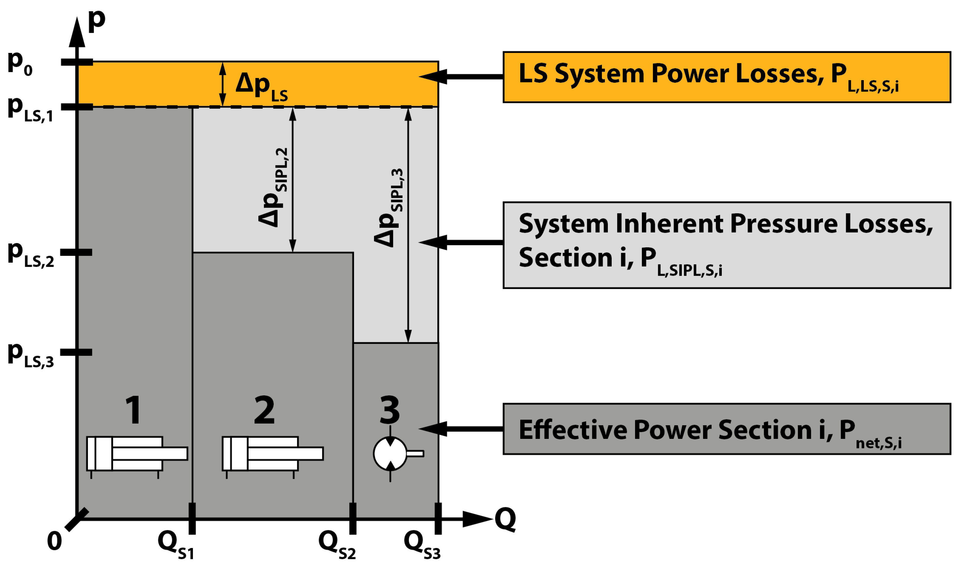
Figure 1 shows a pressure over flow rate (p/Q) diagram of a LS system with three different actuators. As typical for these systems, one actuator, in the given diagram actuator 1, defines the system pressure level supplied by the pump. is defined by the highest load pressure plus the LS pressure difference . Other actuators are supplied with their individual pressure levels (, ) which are lower than . The pressure differences and are caused by throttling at the pressure compensators. Depending on the individual section pressure levels, the pressure differences can be bigger or smaller—nevertheless they are losses and thus will be converted into heat energy, which then has to be taken out of the system again (e.g., via an additional cooling circuit). In dependence of the individual section flow rates and and the section pressure levels, energy losses for each section can be determined.
In this paper, pressure losses due to throttling at individual pressure compensators, which are not compensated by , will be referred to as system inherent pressure losses (SIPL) , see Figure 1.
Figure 1 shows that depending on the type of working activity, or in other words, depending on the kind of work cycle the machine is set to, SIPL can have a significant impact on the machine’s total energy efficiency. However, it can also be seen, that an individual load pressure close to the system pressure level leads to reduced or minimized pressure losses.
Hießl showed in [10] the results of an investigation into how SIPL can be reduced for compact excavators by splitting a single hydraulic circuit into two or even more independent circuits, each equipped with an individual LS pump. The results indicate that the losses of the examined system could be reduced by 22% by adding a second circuit. A third pump would only reduce the losses by about 7%. The potential is with respect to the mean power input. The author came to the conclusion that additional and independent hydraulic circuits can effectively reduce SIPL.
Karvonen also supports in [11] the idea of individual pumps of actuators. By using digital hydraulics, a potential of about 40% of energy savings in total was found. The research shows, that approximately 21% of the savings are achieved by reduced SIPL due to adding independent supply pressures.
Summing up, SIPL occur in all load sensing systems, whenever two or more actuators are being operated simultaneously at different load pressure levels. Bigger pressure differences between the individual load pressure levels cause higher system inherent pressure losses. High SIPL combined with high individual flow rates at the same time lead to considerable energy losses and thus to a poor overall energy efficiency of the examined system. In this paper, a novel hydraulic circuit is introduced, which reduces the system inherent pressure losses by increasing the individual load pressure level and thus reducing SIPL [12,13].
2. Research Project Outline— Approach Description and Structure of the Paper
The paper will show selected results of each step. The structure of the paper is based on the different work packages. The flowchart of Figure 2 depicts the described approach.
First, a thorough investigation into system inherent pressure losses was conducted, cf. Section 3. The aim was to define SIPL, where they occur and to determine the energy improvement potential for a specific machine in a specific work cycle. For the analysis in this paper, machine and cycle data were taken from [14].
After the research, a new hydraulic system with reduced SIPL was developed, see Section 4. In regard to predefined boundary conditions, e.g., compatibility to existing systems, performance or safety criteria, and by using CAE tools, the new circuit was further developed and the important characteristics of all key components were defined. With this first version of the new circuit, simulations were conducted in order to verify the circuit’s functionality and its performance. In this paper, early stage simulation results will not be shown.
In the next step, Section 5, the key component of the new circuit, a special valve referred to as Tank-/Accumulator-Logic Valve (T/A-LV) was developed via simulation. Since no suitable valve was available, a prototype with separate metering edges was developed. The system was examined in simulation and on the test rig. At the end of this step, the simulation model was validated with measurement data from the test rig.
In parallel to the prototype development, a hydraulic LS system test rig was set up, cf. Section 6. The system was designed as a single-circuit LS system with three actuator sections. A simulation model of the test rig was also set up. With the data from the test rig, the simulation model was validated.
Finally, in Section 7 both subsystem simulation models were merged to one optimized LS system. By comparing the simulation results of conventional and optimized LS system with a previously defined reference cycle, the functionality as well as the efficiency improvement potential of the new optimized system was verified.
3. Energy Analysis with Focus on System Inherent Pressure Losses
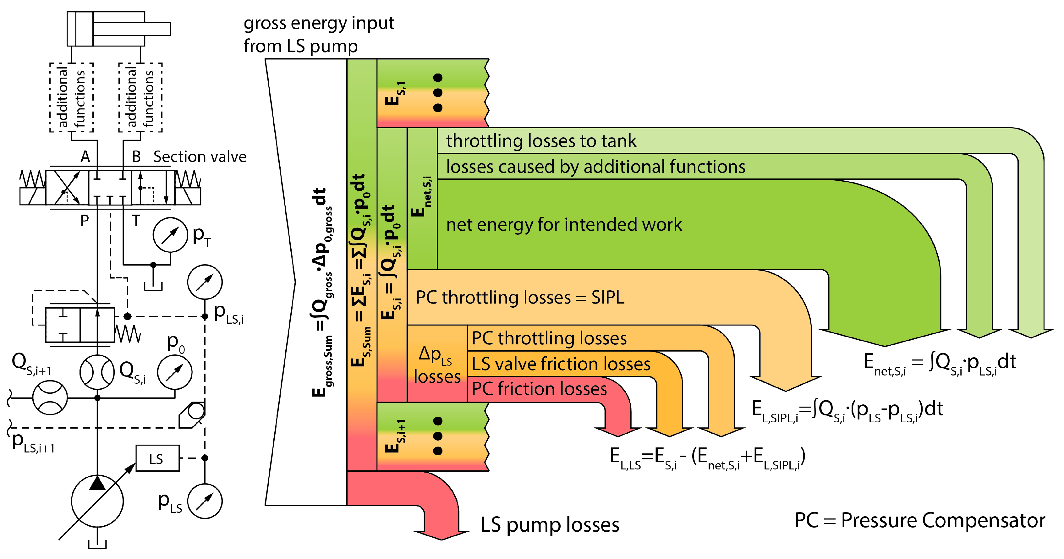
The following section shows the results of an analysis of a 90 degree digging cycle of a hydraulic excavator, taken from [14]. Before the results will be presented, the conducted analysis and the calculated quantities will be defined. Figure 3 depicts the analysis and the calculated energies.
The input of hydraulic energy into the system is referred to as , cf. Equation (1):
is calculated by using the system pressure and the individual flow rates into the load sections, thus neglecting the flow rate required for the pump controller. Pump losses will not be considered in the energy analysis of this paper, because the novel method should not have any influence on either the system pressure level or the system flow rate of the pump. Since both parameters stay the same, the energy input of the pump stays the same and thus the pump controller losses also do. If, however, the proposed method does affect the system pressure level , the additionally required energy has to be considered. does not equal the total input energy from the LS pump , which is shown here due to integrity. Instead, is the sum of all individual section energy requirements .
In each section, (Equation (2)) is the amount of energy, the actuator requires to carry out its designated function, e.g., lifting the boom of an excavator:
This is calculated by using the individual flow rate and the individual load sensing pressure of the section. Thus, always equals zero, whenever the actuator is not moving. It is important to point out, that does not equal the amount of energy, the actuator can use for its intended work function (see Figure 3, arrow labeled “net energy for intended work”). The amount of useable energy always depends on additional valves in the return line and on the load type. Nevertheless, the quantities necessary to calculate can be measured easily and will show changes caused by the proposed efficiency improvement measure.
describes the energy losses due to SIPL in each section, cf. Equation (3):
SIPL are caused by the pressure difference between the individual load sensing pressure level and the system load sensing pressure level . With primary pressure compensators, the calculated pressure difference includes only the pressure difference throttled at the pressure compensator. By using this calculation, effects e.g., caused by undersupply can be omitted. Whenever the system is in undersupply, the pressure difference drops at the section valve with the highest load—this, however, does not affect sections with lower loads.
, Equation (4), describes the losses caused by . It is calculated by subtracting the sum of and from the individual section energy requirements :
To determine the extent of inherent system pressure losses, a 90 degree digging cycle of a hydraulic excavator from [14] will be analyzed according to the previously defined quantities (Figure 3) in the following section. Figure 4 shows the movements of each actuator during the cycle.
The examined machine is a hydraulic crawler excavator with two separate load sensing circuits. Circuit 1 supplies boom and bucket, circuit 2 supplies arm and swing drive of the machine. The synchrony of all movements strongly depends on the skills of the driver, which therefore have a strong influence on the machines efficiency. The cycle data in [14] was generated by a professional driver, therefore the data were considered to be reliable and representative for hydraulic excavators.
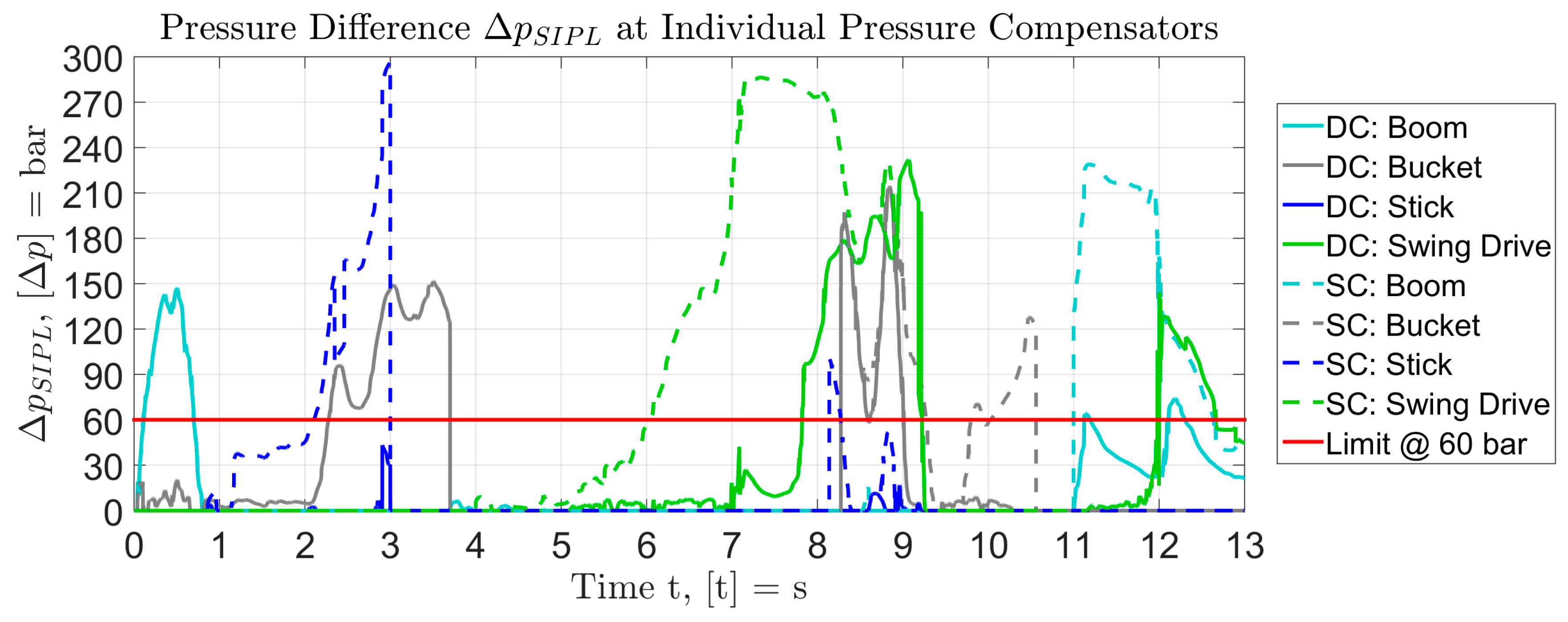
Figure 5 shows the magnitude of the pressure difference of each actuator during the load cycle. The machine was analyzed both in single-circuit (SC) and double-circuit (DC) configuration. The single-circuit data was derived by superposing both circuit LS pressure levels to one pressure trajectory consisting of the maximum pressure level at each time step. In Figure 5, all dashed lines refer to the single-circuit configuration. The red line marks a threshold of 60 bar.
For the boom of the double-circuit machine, the diagram shows that is bigger than 60 bar for approximately 6% with respect to the overall duration of 13 s. For the single-circuit machine, this duration increases up to 17%. All results of the analysis can be seen in Table 1.
Both systems were analyzed using Formulas (1)–(4). The results can be seen in Table 2. Values expressed as a percentage are with respect to in the correlating column.
The comparison shows, that the overall energy consumption of the single-circuit excavator is about 246 kJ higher. In both configurations, remains approximately the same. The difference of both percentage values is owed to the different levels of . The analysis also shows, that for the single-circuit excavator, more than 20% of the total energy input can be considered as system inherent pressure losses in the hydraulic circuit.
4. Development of the Optimized Load Sensing System
Figure 6 shows a p/Q diagram of the optimized LS system with increased load pressure levels and in Section 2 and Section 3.
Due to the new pressure levels, the system inherent pressure losses and thus power losses alike are reduced significantly. However, the individual pressure level cannot be increased up to the highest pressure level, because this would cause instabilities in the system. Increased individual load pressure levels could be achieved, for example, by increasing the work load of the machine (e.g., increasing the mass or density of the material to be moved). However, increasing the external load is not possible, since this would alter the work cycle and thus would leave it incomparable. Other options, e.g., altering the machine’s kinematics will not be considered because of the significant effort.
A more suitable option is to apply an additional pressure potential in the return line, thus clamping the actuator hydraulically. Depending on the type of actuator (double-rod or single-rod cylinder, hydraulic motor) and its pressure intensifying properties, the additional pressure potential in the return line would increase the load pressure in the inlet and thus reduce the pressure difference .
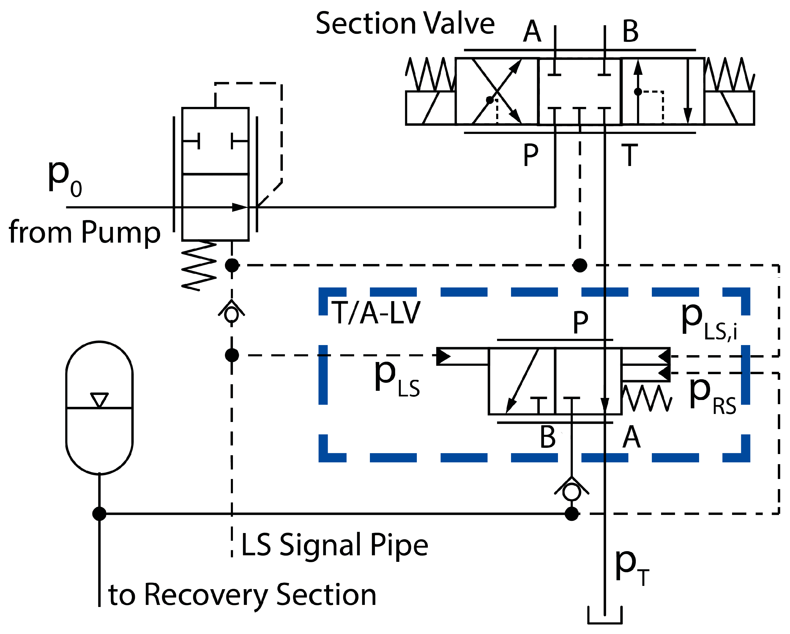
The required pressure potential will be achieved by adding a hydraulic accumulator in the return line. The accumulator however cannot be connected to the return line of all actuators at all times, because otherwise it would simply shift the systems pressure level without the benefits of reducing SIPL. In Figure 7, an optimized LS system with three actuator sections is shown.
Depicted is a conventional LS system with primary pressure compensators. The system is equipped with a variable LS pump and three parallel actuator Sections (A1–A3). Furthermore, each section is equipped with an additional 4/3 proportional spool valve. The return line of each section is not connected directly to the tank but to the Tank-/Accumulator-Logic Valve (T/A-LV). The valve itself is connected to the tank and the Recovery Section (RS). Following upstream, the RS itself consists of a check valve for each section, a hydraulic accumulator and the Recovery Unit (RU). The depicted RU basically has two tasks: it has to transform hydraulic energy into mechanical energy and reroute it back into the system, for example by way of an additional momentum applied at the shaft of the ICE. By doing so, the RU fulfills its second main task and allows for the needed pressure potential to build up.
The key component of the optimized system is the T/A-LV. In Figure 7, the valve is implemented as a 3/2 proportional spool valve with hydraulic actuation and a specific edge characteristic. It has three main tasks: with its control surfaces, the valve has to determine the individual load situation of its actuator section and then, depending on it, connecting the section return line either to the tank or to the RS. The valve furthermore has to allow for a smooth and vibration free shifting motion, so that the performance of the entire systems does not deteriorate.
Figure 8 depicts the T/A-LV in a more detailed way. As previously mentioned, the valve has three different hydraulic control surfaces which are connected to the pressure potentials , and . The valve also has a spring counteracting .
For the valve, either proportional or switching (I/O) motion is conceivable. In the project, a proportional valve was chosen. Depending on the equilibrium of forces at the spool, the connection between return line and tank can be throttled, which automatically leads to a higher pressure in the return line.
By calculating the equilibrium of forces for the valves spool, Equation (5) can be derived, where is the pressure of the LS system, is the pressure in the recovery section, is the control surface, is the individual load pressure and is the spring force. The factor is the surface ratio of the connected differential cylinder. For a double-rod cylinder or a hydraulic motor equals one, otherwise is always bigger than one:
Using (5) and , three different cases can be identified, which will be described in the following paragraphs:
Case 1, Equation (6), applies to all actuators with high or the highest loads. When an actuator fulfills this condition, raising the return line pressure would automatically alter the system pressure level and would increase energy losses unnecessarily. Thus for Case 1, system inherent pressure losses cannot be reduced. To prevent this situation from happening, the return line of the actuator with the highest load needs to be connected to the tank entirely.
Case 2, Equation (7), defines the threshold Equation (5). In this case, pressure forces on both sides of the spool create an equilibrium. The valve throttles the return line flow rate, increases the return line pressure and thus affects the individual load pressure of the actuator. Thus, the pressure losses at the pressure compensators are reduced already. Nevertheless, in Case 2 the return line pressure is still lower than the pressure in the RS and therefore no energy can be recovered. All recoverable energy is being throttled at the valve in the return line.
When an actuator of lower load satisfies the condition of Case 3, Equation (8), loss energy can be recovered. The T/A-LV tank edge is closed completely so that the return line of the actuator is fed into the recovery unit. The pressure in the recovery section now directly counteracts the supply pressure of the connected actuator(s), thus increasing the section pressure [15].
5. Development of the Tank-/Accumulator-Logic Valve (T/A-LV)
The following section describes the development of the key component T/A-LV. During the research project, no valve was available on the market, which could be used as a T/A-LV substitute.
Since the valve is crucial to the new circuit, a valve prototype was developed with separate metering edges and software open and closed loop control. Using separate metering edges offered considerable benefits: Combined with software valve control, separate metering edges are very flexible as hardware components. Furthermore, they do provide a very easy way to change valve parameters, such as valve characteristics, control surface ratios, spring stiffness etc. Figure 9 depicts the scheme of the T/A-LV prototype.
Unlike the original valve, the prototype consisted of two separate proportional throttle valves, which were connected by hydraulic tubes and hoses. Each throttle valve was controlled individually by the valve control hardware, a rapid prototyping computer (RPC, Autobox, dSPACE). The RPC was connected to the valves via a power amplifier and to all sensors. Since the prototype did not have the necessary control surfaces, pressure transducers were used for each required pressure level , and . Furthermore, the RS was equipped with flow rate sensors.
The valve control software was programmed in Matlab/Simulink. In the program, all necessary parameters, such as control surface diameters, spring data and edge characteristics were defined. The software used Equation (5) and all available valve and system parameters to compute the necessary valve signals for each metering edge.
5.1. T/A-LV Prototype: Return Line Pressure Control Valve with State Based Controller
For the control concept of the prototype, a state-based logic controller was used to detect the load condition of the actuator section (see also Section 4, Equations (6)–(8) and Figure 10).
The valve controller compares pressure levels , and by using Equation (6). Depending on the results, cases 1 to 3 was identified and the two metering edges were controlled accordingly.
The RS edge was opened completely all the time. Due to the check valve, closing the connection between the return line and the RS was not necessary. A load according to case 1 opened the tank edge completely, a load according to case 3 closed it completely. Whenever the load does not match either case 1 or case 3, a load according to case 2 was assumed. In this situation, the tank edge throttled the return flow rate in order to raise the return line pressure. The tank edge was controlled in closed loop by a PID controller, which was used to increase the return flow pressure as much as possible without switching the load case. The intention of the PID was to allow for a gradual load case transition.
5.2. T/A-LV Prototype: Development and Testing
The previously described concept was developed by simulation and tested on a test rig (see Figure 11). The simulation model was set up like the test rig and thus will not be depicted here. For the simulations the softwares DSHplus 3.9.2 and Matlab/Simulink were used. For further information, see also [9].
The test rig was designed as a single LS section. To apply load, a proportional pressure relief valve was used (PPRV-1). The valve was controlled in open loop. The flow rate of the section was adjusted by the section valve, a standard load sensing manifold for mobile hydraulics, provided by the company HYDAC (Sulzbach, Saar, Germany). The manifold was equipped with a primary pressure compensator. The system was pressurized by the central pressure supply (CPS) of Mobima. As it can be seen in Figure 11, the supply pipe of the CPS was connected to the LS port of the manifold. Therefore, the section could be operated like a section with lower load in a multi section LS system. Downstream of PPRV-1, an additional pressure relief valve (PRV-1) was added for safety reasons. The two proportional throttle valves SME-R/T and SME-R/RS were the T/A-LV prototype. Each valve was equipped with an individual flow rate sensor (Q2, Q3). While SME-R/T was connected to the tank, SME-R/RS was connected to the hydraulic accumulator and another proportional pressure relief valve (PPRV-2) via a check valve. The combination of the hydraulic accumulator and PPRV-2 represented the RS of the test rig, thus establishing the adjustable and raised pressure level in the RS. Four pressure transducers were used to measure the system pressure (p1 or ), the individual load pressure (p2 or ), the return line pressure (p3) and the RS pressure (p4 or ). Characteristics of the used sensors are listed in Table 3.
Prior to the experiment, the accumulator was charged with approximately 60 bars, PPRV-2 was set to a pressure of 60 bars as well. The section valve was set to a fixed flow rate of approximately 20 L/min in order to keep friction losses due to oil flow to a minimum. The CPS was set to keep a constant pressure level of 200 bars. PRV-1 was set to a pressure of around 300 bars. SME-R/RS was set to fully opened position. Temperature was not measured in the system.
During the used cycle, the individual section load would increase and decrease and thus changing from load case 3 (recover energy, Equation (8)) to case 2 (throttled return line, Equation (7)), to case 1 (not throttled return line, Equation (6)) and then back to case 3.
Figure 12 shows the smoothed result of the verification experiment. In the upper part of the diagram, the measured system pressure p1 (CPS, blue dashed line, ![Energies 10 00941 i001]() ), the measured section pressure p2 (black line,
), the measured section pressure p2 (black line, ![Energies 10 00941 i002]() ), the signal of the nominal load pressure (green line,
), the signal of the nominal load pressure (green line, ![Energies 10 00941 i003]() ), the return line pressure p3 (red dash-dotted line,
), the return line pressure p3 (red dash-dotted line, ![Energies 10 00941 i004]() ) and the predicted section pressure (orange dash-double-dotted line,
) and the predicted section pressure (orange dash-double-dotted line, ![Energies 10 00941 i005]() ) can be seen. Figure 12 (bottom) shows the measured flow rate Q1 (black line,
) can be seen. Figure 12 (bottom) shows the measured flow rate Q1 (black line, ![Energies 10 00941 i002]() ) and the predicted flow rate (orange dash-double-dotted line,
) and the predicted flow rate (orange dash-double-dotted line, ![Energies 10 00941 i005]() ). In the diagram, predicted trajectories show what the measured trajectories of the corresponding values were expected to look like. From the beginning of the measurement until 9.5 s, the section load pressure is increased by the pressure level of the RS (approx. 60 bar), meaning that even with the load applied by PPRV-1, valve SME-R/T is closed and the entire flow rate runs through the RS.
). In the diagram, predicted trajectories show what the measured trajectories of the corresponding values were expected to look like. From the beginning of the measurement until 9.5 s, the section load pressure is increased by the pressure level of the RS (approx. 60 bar), meaning that even with the load applied by PPRV-1, valve SME-R/T is closed and the entire flow rate runs through the RS.
 ), the measured section pressure p2 (black line,
  ), the signal of the nominal load pressure (green line,
  ), the return line pressure p3 (red dash-dotted line,
  ) and the predicted section pressure (orange dash-double-dotted line,
  ) can be seen. Figure 12 (bottom) shows the measured flow rate Q1 (black line, ) and the predicted flow rate (orange dash-double-dotted line, ). In the diagram, predicted trajectories show what the measured trajectories of the corresponding values were expected to look like. From the beginning of the measurement until 9.5 s, the section load pressure is increased by the pressure level of the RS (approx. 60 bar), meaning that even with the load applied by PPRV-1, valve SME-R/T is closed and the entire flow rate runs through the RS.
At about 9.5 s, the applied load starts to increase and the section pressure increases alike. The volume flow decreases slightly, but stays almost constant until 9.8 s. At about 9.8 s, load case 3 changes to load case 2, which means, section pressure cannot be increased by the RS pressure level without changing the systems’ pressure. Therefore, the connection between return line and tank needs to open, which can be seen in the period from roughly 10.2 s to 12 s.
Beginning at app. 9.8 s, predicted and measured p2 start to differ. The predicted pressure shows a reduction, beginning at app. 9.8 s, after which, app. 10.3 s, predicted and nominal pressure are at the same level. The predicted flow rate Q1 remains the same during the entire period. The experiment however shows, that p2 almost reaches the systems pressure level and thus the flow rate almost drops to zero (at approx. 10.2 s).
The reason for this behavior is valve SME-R/T, which is too slow and cannot open the connection as fast as required. Therefore, flow rate drops and the section pressure rises almost to system pressure level. At this point, the fact that the test rig was pressurized by a CPS with closed-loop pressure control needs to be highlighted again. If the examined sections were part of a real load sensing system, the flow rate would not change (considerably). Instead, the system pressure would rise up to the necessary level to keep the volume flow at the desired rate. The CPS however reduces the flow because of the closed loop pressure control.
Beginning at 10.2 s, the flow starts to increase again and p2 starts to drop gradually. At 12.2 s, the nominal load drops again and the flow rate returns to its nominal level. The experiment shows that the T/A-LV prototype was operational, but too slow to provide the required level of dynamic pressure adjustment at that time. The reduced dynamics were a result of different tests on the test rig. In order to establish vibration reduced operation, the valve signals had to be filtered and damped, thus reducing the dynamics of the valve control.
6. Load Sensing System Test Rig
6.1. Test Rig Configuration
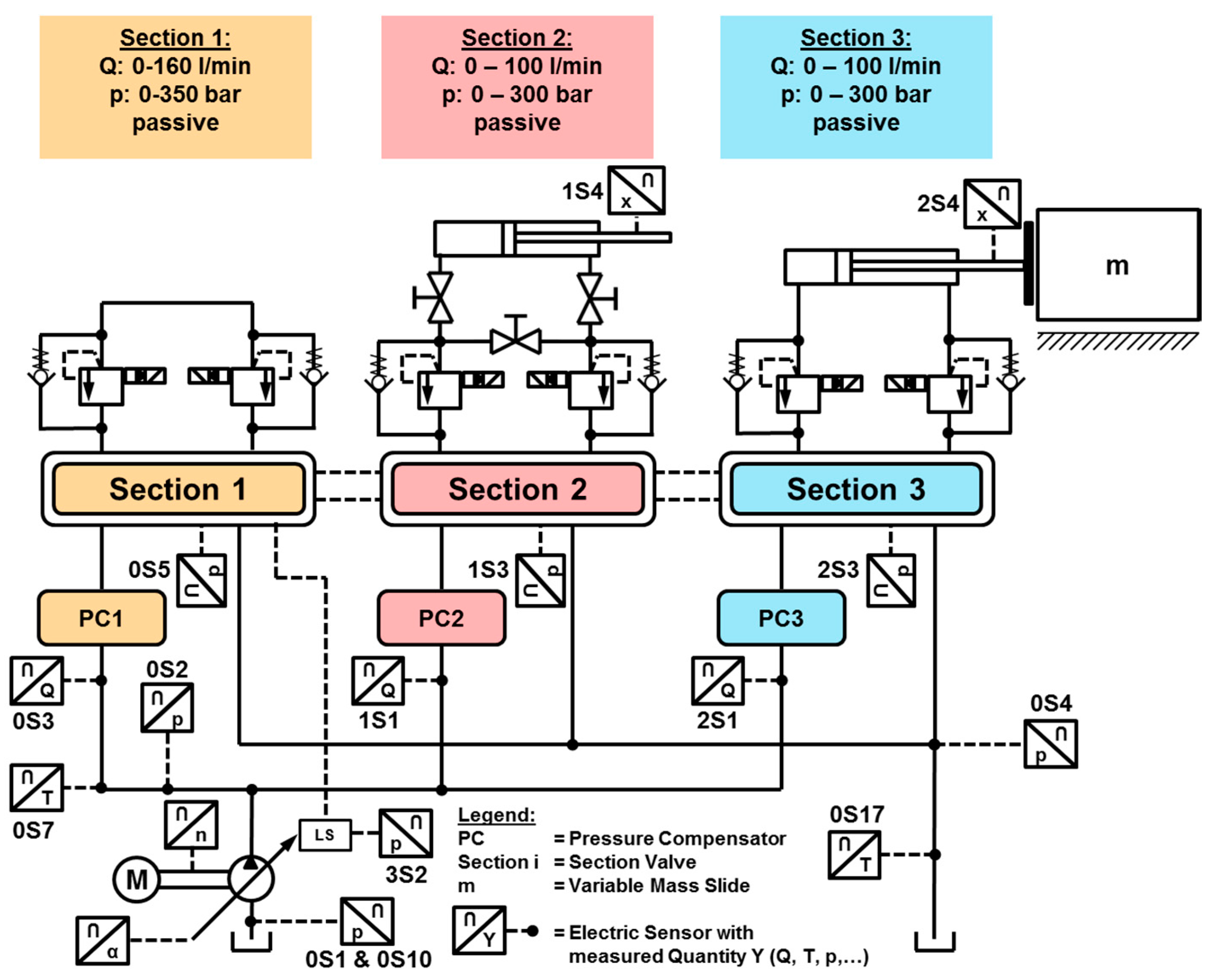
Figure 13 shows the scheme of the test rig in the project. The test rig was designed as a single-circuit LS system with three different actuator sections. The following section briefly describes the test rig and the used components – a more detailed description can be found in [9].
The test rig was equipped with a variable displacement swashplate pump, A11VO from Bosch Rexroth (Elchingen, Germany), with 95 cm³ max. stroke volume, a standard LS flow controller and a hydraulic power of up to 128 kW. The pump was driven by an electric asynchronous motor with 130 kW peak power. It was fed by the CPS of Mobima with Renolin B 15 VG 46. Therefore, the test rig did not require any additional components such as cooling and filtering circuits.
The LS manifolds (LS manifold Type LX6) were provided by HYDAC. The valves were equipped with primary pressure compensators and electric valve control. As it can be seen in Figure 13, the three load sections were separated from each other. Each manifold consisted of one single working section with an individual inlet and end plate. This setup was necessary so that all individual volume flows and pressures could be measured.
The test rig was controlled by RPC AutoBox from dSPACE (Paderborn, Germany). As common for mobile hydraulics, all valves were connected via a CAN network with components from IFM. The GUI of the test rig was implemented in ControlDesk, dSPACE and allowed for manual as well as for automated operation with time based open and closed loop cycle control for all components.
Three separate load sections were set up. For each section, load could be applied by downstream electrohydraulic proportional pressure relief valves (PPRV). Each section had a different purpose. Section 1 (Figure 13, left) only consisted of two downstream PPRVs, connected with tubes and hoses. It could be used to simulate a hydraulic motor, or simply another actuator with passive loads.
Section 2 and Section 3 were equipped with hydraulic cylinders each. In addition, the cylinder of Section 3 was connected to a mass slide to simulate inertia. Both cylinders could be charged by downstream PPRVs. For Section 3, a separate active load unit was in planning, but has not been finished. Thus, only passive loads could be applied at the test rig.
A number of sensors were installed in the test rig in order to gather all necessary data. The asynchronous motor of the LS pump was equipped with an rpm-/torque sensor. The LS pump was equipped with a swash plate angle sensor, a pressure transducer at the tank port, at the LS port and at the high pressure port. Each load section had its own flow rate sensor and LS pressure transducer. In Section 2 and Section 3, laser position sensors were attached to the pistons of the cylinders. In the high pressure gallery as well as in the test rig return line, temperature was measured. Furthermore (not depicted in Figure 13), leakage pressure of the LS manifolds and the LS pump and the supply pressure of the CPS were measured due to safety reasons.
Characteristics of the used sensors can be found in Table 4. Sensors without label in Figure 13 were not needed for the following results and will not be discussed further. The analyzed cycle was derived from the 90 degree digging cycle data from [14]. The reference system, a hydraulic excavator (1804 LC, Atlas, Ganderkesee, Germany) with about 125 kW, and the target system, the test rig, were in the same power level, however the Atlas 1804 LC had a double-circuit hydraulic LS system. Therefore and due to safety reasons the reference cycle was scaled and adjusted to a reduced power level. By superposing the pump pressure data of both circuits and taking the maximum pressure value each time, the double-circuit system was altered to a single-circuit system. For flow rate, the individual circuit flow rates were added up to a sum flow rate. Thus, the new single-circuit system supplied the previously described pressure trajectory and the cumulative flow rate. Then, the maximum flow rate and pressure values were scaled to match the dimensions of the test rig. Finally, the overall cycle time was increased in order to allow for easier measurement and cycle control. All cylinder movements were scaled equally, thus keeping the precentral distance alike.
6.2. Validation of the Test Rig Simulation Model
Measured data of the test rig are used to validate the simulation model of a conventional LS system. The simulation model is set up like the test rig (see Figure 13) with DSHplus 3.9.2 (Fluidon, Aachen, Germany). All model parameters are taken either from available datasheets of the used components, calculated or derived from single component experiments on the test rig. The parameters of the fluid are set in accordance with the parameters of the fluid in the test rig.
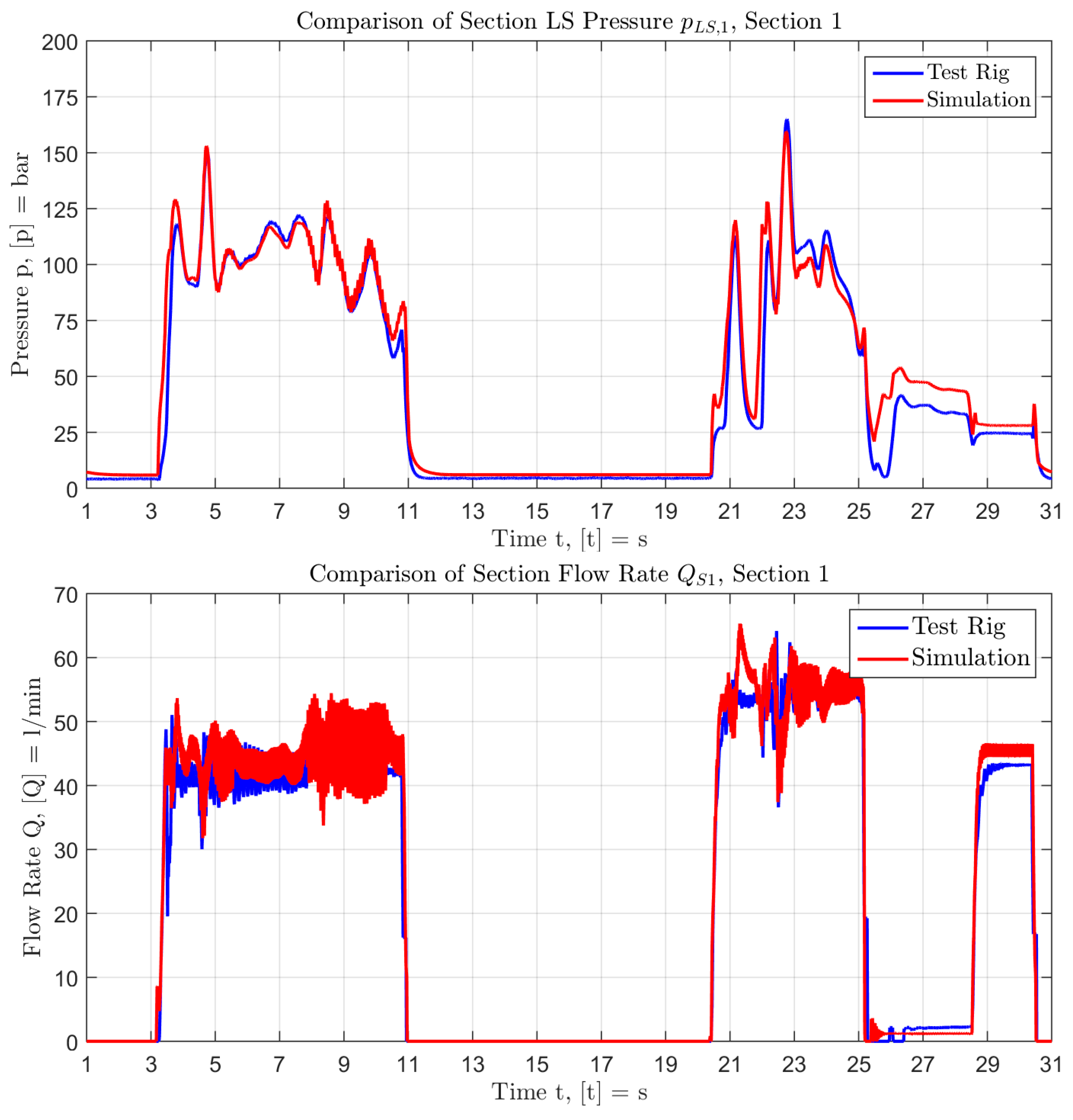
Figure 14 (top) compares the simulated (red line) and measured (blue line) of Section 1. Between 25 s and approximately 29 s pressure deviations of about 10–15 bar are visible. This is caused by unprecise parameterization of the section valves characteristic. For flow rate (see Figure 14 (bottom)), the simulation and measurement differ by approximately 5 L/min. The highest deviations are between 20 s and 25 s. For , the median absolute deviation is 1.6 bars with a median of −1.6 bars. For , is 2.6 L/min with a median of −1.9 L/min.
Figure 15, Figure 16, Figure 17 and Figure 18 display the validation results. Figure 15 depicts the same analysis for Section 2. has a of 0.8 bar with a median of -0.1 bar. The of equals to 1.5 L/min with a median of −0.1 L/min. In addition, in Figure 16 the cylinder position is shown. At the end of the cycle, the simulated cylinder position differs by less than 10 mm.
Figure 17 shows , calculated according to Equation (1). During the simulated load cycle, the simulation requires about 10 kJ more energy than the test rig, which is less than 4% of the overall energy consumption. Thus, the simulation model is considered as valid.
7. Validation of the Optimized Load Sensing System
The simulation model of the test rig and of the T/A-LV prototype were integrated into one simulation model of the optimized LS system, cf. Figure 18.
The individual return lines were equipped with the simulation model of the T/A-LV prototypes. Also the implemented valve control was added. Furthermore, the system was equipped with the RS, consisting of an accumulator and a proportional pressure relief valve.
For the final analysis, the reference cycle (see also Section 6.1) was simulated with the conventional and the optimized LS system model. Afterwards, both results were compared. The simulation model was set up in DSHplus 3.9.2 and controlled by Matlab/Simulink.
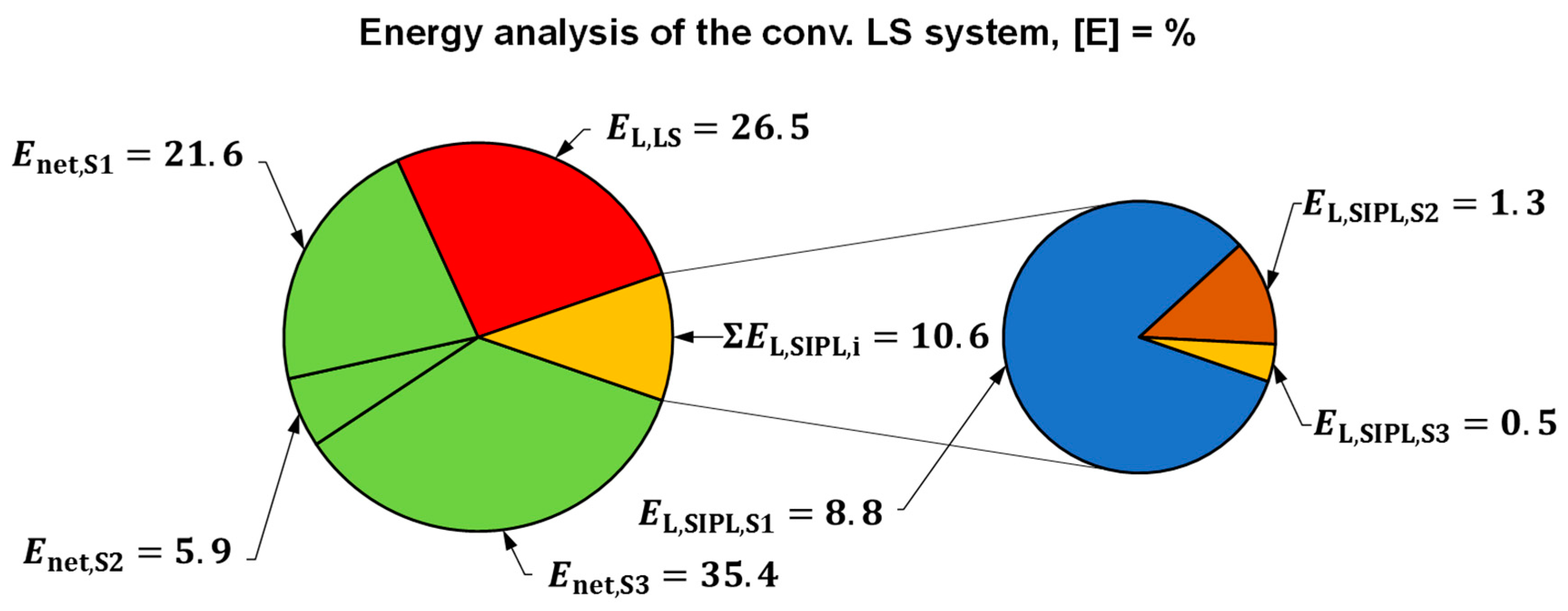
The results of the reference cycle analysis can be seen in Figure 19. The pie chart shows that approximately 37% of the energy input are losses during the load cycle. Almost 11% of these losses are system-inherent pressure losses (Figure 19, sum of SIPL). The big share of is caused by a high of about 30–40 bar, which was necessary for the test rig in order to reduce vibrations in Section 1.
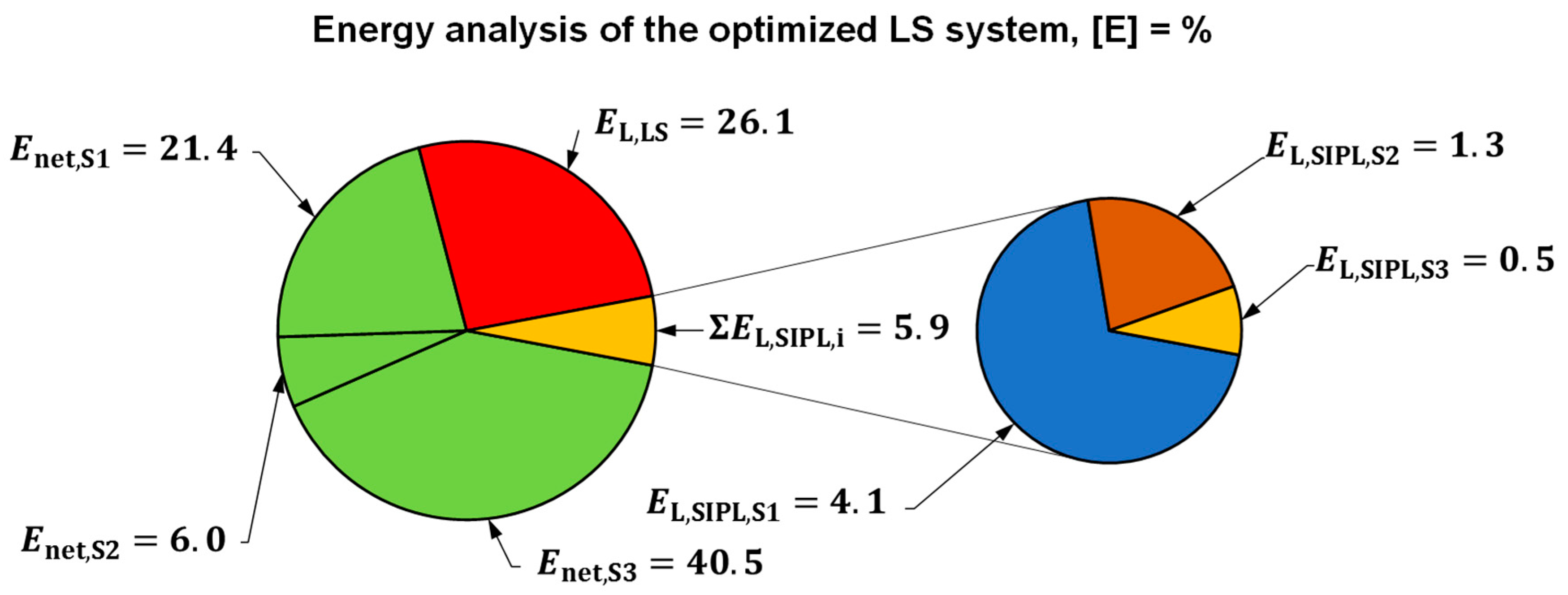
In Figure 20, the results of the analysis of the optimized LS system can be seen. The diagram shows that the sum of SIPL in Section 1 was reduced by almost 44 %. The reduction in other sections was very small and therefore neglected due to the chosen precision.
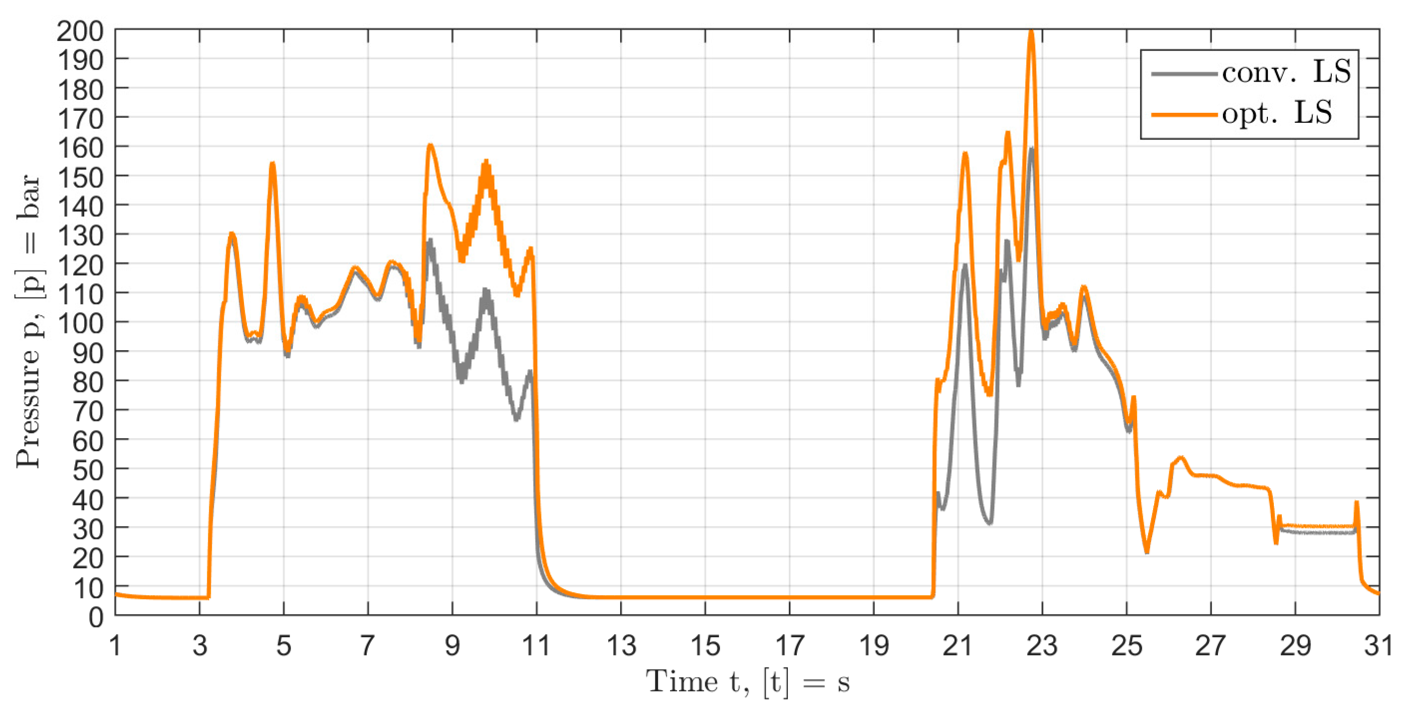
Figure 21 and Figure 22 compare the optimized and the conventional LS system. Figure 21 depicts the systems LS pressure and Figure 22 the section LS pressure , in Section 1. From beginning of the cycle until approximately 21 s, of the optimized and the conventional system match, with the LS pressure of the optimized system being slightly higher (≤3 bar). This is owed to the fact, that after adding the T/A-LVs all sections have additional friction losses in the return line. Between app. 8 s and 11 s (Figure 22) the individual section pressure of Section 1 of the optimized LS is raised by 50–60 bar compared to the conventional system, caused by the T/A-LV and a successful connection to the RU. Between 20 s and 23 s the pressure is also raised, but as it can be seen in Figure 21, the systems LS pressure is affected as well. While the first raise means reduced losses, the second raise leads to increased losses of the optimized system. The analysis of other results implicate, that this behavior is caused by the unsatisfactory dynamics of the T/A-LV prototypes and thus could be reduced by optimization loops.
Summing up, the comparison of both systems shows, that the proposed optimization measure can reduce the system inherent pressure losses of a conventional LS system. The experiment showed a pressure loss reduction of approximately 44% in the reference cycle.
With respect to the overall energy consumption of the system, this decrease correlates to a efficiency improvement of around 2%. Although modest, the result shows, that system inherent pressure losses can be reduced and do hold a considerable potential for efficiency improvement. As previously described, the potential of the proposed measure strongly depends on the share of system inherent pressure losses in the analyzed work cycle, in this case, the reference cycle. The results in [11] support this assumption as well.
Furthermore, optimizing the dynamics of the T/A-LV is also likely to have a certain influence on the efficiency improvement potential. This assumption is supported by the fact, that between 20 s and 23 s, cf. Figure 22, the system LS pressure level is affected and thus the energy input from the pump. However, this has not yet been analyzed further.
8. Conclusions
In this paper, a novel method of improving the efficiency of LS systems was introduced. The proposed approach led to increased efficiency of the system due to reduced system inherent pressure losses. In order to do this, a conventional LS system was equipped with the developed hydraulic circuit and all mentioned components: The Tank-/Accumulator-Logic Valve (T/A-LV), the Recovery Section (RS) and all required piping.
So far, a circuit was developed in simulation and investigated thoroughly. Simulation results showed, that the proposed circuit reduced the system inherent pressure losses of the examined hydraulic LS system. However, the parameters of the T/A-LV and especially its dynamics were of the essence and required further optimization.
In the paper, a T/A-LV prototype with separate metering edges and a software valve control was described, which was used to do research on the real valve. The prototype was implemented successfully on a test rig and a valid simulation model was set up. Nevertheless, the system required optimization.
To gather good evidence, a hydraulic LS test rig was set up and tested. The system of the test rig was designed like a single-circuit LS system of a hydraulic excavator. Also, a simulation model of the test rig was set up, which then was validated with measured data.
By combining the T/A-LV model and the conventional LS model, a simulation model of the optimized hydraulic system was implemented. Conducted simulations with the model of the optimized system and a derived reference load cycle showed a reduction of system inherent pressure losses of approximately 44%. Thus, despite of the unsatisfactory dynamic properties of the T/A-LV prototype, the proposed approach of reducing system inherent pressure losses can contribute to efficiency improvement of mobile machines. Further investigations related to the topic are planned.
Acknowledgments
All research and proceedings were part of the research project “Reduzierung systembedingter Energieverluste an Druckwaagen in Load-Sensing-Systemen durch Reihenschaltung eines Hydrospeichers” (Reduction of system inherent energy losses at pressure compensators of load sensing systems by means of serial connection to a hydraulic accumulator), which was conducted from October 2013 to June 2016 at the Institute of Mobile Machines (Mobima) of the Karlsruhe Institute of Technology (KIT). The project, FKM number 703050, was directly funded by the Forschungsfonds Fluidtechnik (Research Fund Fluid Power, FFF) of the Verband Deutscher Maschinen und Anlagenbau (Mechanical Engineering Industry Association, VDMA, Germany). The FFF is a member of the Forschungskuratorium Maschinenbau e.V. (FKM). Further information about the project can be found in [9]. The authors would especially like to thank the Companies Bosch Rexroth, Bucher Hydraulics GmbH, Hawe Hydraulik SE and HYDAC INTERNATIONAL GmbH. The authors furthermore acknowledge support by Deutsche Forschungsgemeinschaft and Open Access Publishing Fund of Karlsruhe Institute of Technology.
Author Contributions
Jan Siebert was leading researcher on the described project and wrote the paper. Marco Wydra developed the software control of the T/A-LV prototype and did the testing on the test rig. Marcus Geimer supervised the project as head of the Institute of Mobile Machines of the KIT in Karlsruhe.
Conflicts of Interest
The authors declare no conflict of interest.
Nomenclature
| Acronyms | |
| CAE | Computer Aided Engineering |
| CAN | Controller Area Network |
| CPS | Central pressure supply of Mobima/KIT |
| DC | Double-circuit |
| GUI | Graphical user interface |
| ICE | Internal combustion engine |
| LS | Load-Sensing |
| PC | Pressure controller |
| PPRV | Proportional pressure relief valve |
| PRV | Pressure relief valve |
| RPC | Rapid prototyping computer |
| RS | Recovery section |
| RU | Recovery Unit |
| SC | Single-circuit |
| SIPL | System inherent pressure losses |
| SME-R/RS | Separate metering edge, connecting return line with the recovery section |
| SME-R/T | Separate metering edge, connecting return line with the tank |
| T/A-LV | Tank-/Accumulator-Logic Valve |
| Symbol | Unit | Description |
| α | deg | Angle position of swing drive |
| mm² | Hydraulic control surface of a valve connected to pressure | |
| mm² | Hydraulic control surface of a valve connected to pressure | |
| mm² | Hydraulic control surface of a valve connected to pressure | |
| bar | Median absolute deviation, unit depending on the quantity referred to | |
| kJ | Energy input from LS pump of the system | |
| kJ | Energy of losses due to | |
| kJ | Energy losses due to system inherent pressure losses, section i | |
| kJ | Energy necessary in section i to carry out the designated work function | |
| kJ | Individual energy requirement of section i | |
| kJ | Input of hydraulic energy into a hydraulic system | |
| N | Spring force | |
| M | kg | Mass |
| bar | System pressure level of a Load-Sensing system | |
| bar | Pressure input from LS pump | |
| bar | Individual LS pressure level of section i | |
| bar | System LS pressure, defined by section with highest load | |
| bar | Pressure level of recovery section | |
| bar | Pressure equivalent of spring force | |
| bar | Pressure in tank | |
| l | bar | LS pressure difference at flow control valve of the LS pump |
| l | bar | Pressure difference of system inherent pressure losses at section i |
| W | Hydraulic power | |
| W | Mechanical power | |
| W | Power referring to , section i | |
| W | Power referring to | |
| W | Power referring to of section i | |
| W | Individual power of section i | |
| L/min | Flow rate, system input | |
| L/min | Recovered flow rate | |
| l | L/min | Flow Rate in return line |
| L/min | Flow rate, section i | |
| t | s | Time |
| x | mm | Position of cylinder |
| 1 | Surface ratio of a differential cylinder |
References
- Findeisen, D.; Helduser, S. Ölhydraulik: Handbuch für die hydrostatische Leistungsübertragung in der Fluidtechnik, 5th ed.; Springer: Berlin/Heidelberg, Germany, 2006; p. 32. [Google Scholar]
- Inderelst, M. Efficiency Improvements in Mobile Hydraulic Systems. Ph.D. Thesis, IFAS/RWTH Aachen, Aachen, Germany, 5 Februrary 2013. [Google Scholar]
- Joo, C.; Stangl, M. Application of Power Regenerative Boom system to excavator. In Proceedings of the 10. IFK: International Fluid Power Conference, Dresden, Germany, 8–10 March 2016; Dresdner Verein zur Förderung der Fluidtechnik e.V. Dresden: Dresden, Germany, 2016; Volume 3, pp. 175–184. [Google Scholar]
- Caterpillar Machine Product & Service Annoucements. Cat® 336E H Hydraulic Hybrid Excavator Delivers No-Compromise, Fuel-Saving Performance. Available online: http://www.cat.com/en_IN/news/machine-press-releases/cat-sup-174-sup-336ehhydraulichybridexcavatordeliversnocompromis.html (accessed on 16 May 2017).
- Lettini, A.; Havermann, M.; Guidetti, M.; Fornaciari, A. Electro-Hydraulic Load Sensing: A Contribution to Increased Efficiency through Fluid Power on Mobile Machines. In Proceedings of the 7. IFK: International Fluid Power Conference, Aachen, Germany, 22–24 March 2010; Apprimus Verlag: Aachen, Germany, 2010; Volume 3, pp. 103–114. [Google Scholar]
- Grösbrink, B.; Stamm von Baumgarten, T.; Harms, H.-H. Alternating Pump Control for a Load-Sensing System. In Proceedings of the 7. IFK: International Fluid Power Conference, Aachen, Germany, 22–24 March 2010; Murrenhoff, H., Ed.; Apprimus Verlag: Aachen, Germany, 2010; Volume 3, pp. 139–150. [Google Scholar]
- Axin, M. Mobile Working Hydraulic System Dynamics. Ph.D. Thesis, Division of Fluid and Mechatronic Systems/Department of Management and Engineering/Linköping University, Linköping, Sweden, August 2015. [Google Scholar]
- Scherer, M. Beitrag zur Effizienzsteigerung mobiler Arbeitsmaschinen: Entwicklung einer elektrohydraulischen Bedarfsstromsteuerung mit aufgeprägtem Volumenstrom. Ph.D. Thesis, Institute of mobile Machines, Karlsruhe Institute of Technology, Karlsruhe, Germany, January 2015. [Google Scholar]
- Siebert, J.; Geimer, M. Abschlussbericht zum Forschungsvorhaben: Reduzierung systembedingter Druckverluste an Druckwaagen von Load-Sensing-Systemen durch Reihenschaltung eines Hydrospeichers (RSD); Direktgefördertes Forschungsprojekt FKM-Vorhaben Nr. 703050 der Forschungsvereinigung Forschungskuratorium Maschinenbau e.V.: Karlsruhe, Germany, 2016. [Google Scholar]
- Hießl, A.; Scheidl, R. Methodical Loss Reduction in Load Sensing Systems Based on Measurements. In Proceedings of the BATH/ASME 2016 Symposium on Fluid Power and Motion Control, Bath, UK, 7–9 September 2016. [Google Scholar]
- Karvonen, M. Energy Efficient Digital Hydraulic Power Management of a Multi Actuator System. Ph.D. Thesis, Tampere University of Technology Publication, Tampere, Finland, 2016. [Google Scholar]
- Nagel, P. Hydraulisches Mehrverbrauchersystem Mit Energieeffizienter Hydraulischer Schaltung. Patent EP20140705278, 7 August 2014. [Google Scholar]
- Geimer, M. Projektantrag: Reduzierung systembedingter Energieverluste an Druckwaagen von Load-Sensing-Systemen durch Reihenschaltung eines Hydrospeichers (RSD); Eingereicht beim Forschungsfonds Fluidtechnik (FFF) des Verband Deutscher Maschinen und Anlagenbau (VDMA): Karlsruhe, Germany, 2013. [Google Scholar]
- Holländer, C. Untersuchung zur Beurteilung und Optimierung von Baggerhydrauliksystemen. Ph.D. Thesis, Technische Universität Braunschweig, Braunschweig, Germany, 1998. [Google Scholar]
- Siebert, J.; Geimer, M. Reduction of System Inherent Pressure Losses at Pressure Compensators of Hydraulic Load Sensing Systems. In Proceedings of the 10. IFK: International Fluid Power Conference, Dresden, Germany, 8–10 March 2016; Dresdner Verein zur Förderung der Fluidtechnik e.V. Dresden: Dresden, Germany, 2016; Volume 1, pp. 253–266. [Google Scholar]
- Wydra, M. Projekt RSD: Übertragung der Charakteristik des Tank-/Speicher-Logikventils auf Ein System Mit Aufgelösten Steuerkanten. Master’s Thesis, Lehrstuhl für Mobile Arbeitsmaschinen (Mobima), Karlsruhe, Germany, 2016. [Google Scholar]
- Siebert, J.; Geimer, M. Entwicklung eines effizienzgesteigerten Load-Sensing-Systems für mobile Arbeitsmaschinen durch Reduzierung systembedingter Druckverluste. In Proceedings of the 9. Kolloquium Mobilhydraulik, Karlsruhe, Germany, 22–23 September 2016. [Google Scholar]
Figure 1.
p/Q diagram of a LS system with three different actuators [9]. Reproduced with permission from the publisher.
Figure 1.
p/Q diagram of a LS system with three different actuators [9]. Reproduced with permission from the publisher.

Figure 2.
Flowchart of the research project.

Figure 3.
Energetic analysis of a hydraulic LS system, as used in the research project.

Figure 4.
90 Degree digging cycle of a hydraulic excavator, Data taken from [14].
Figure 4.
90 Degree digging cycle of a hydraulic excavator, Data taken from [14].

Figure 5.
Analysis of 90 degree digging cycle, pressure difference at pressure compensators.

Figure 6.
p/Q diagram with reduced system inherent pressure losses [9]. Reproduced with permission from the publisher.
Figure 6.
p/Q diagram with reduced system inherent pressure losses [9]. Reproduced with permission from the publisher.

Figure 7.
Load sensing system in optimized configuration. Previously disclosed in [15]. Reproduced with permission from the publisher.
Figure 7.
Load sensing system in optimized configuration. Previously disclosed in [15]. Reproduced with permission from the publisher.

Figure 8.
New circuit with T/A-LV in detail. Previously presented in [15]. Reproduced with permission from the publisher.
Figure 8.
New circuit with T/A-LV in detail. Previously presented in [15]. Reproduced with permission from the publisher.

Figure 9.
Scheme T/A-LV prototype. Previously published in [15]. Reproduced with permission from the publisher.
Figure 9.
Scheme T/A-LV prototype. Previously published in [15]. Reproduced with permission from the publisher.

Figure 10.
T/A-LV Logic Chart (see also [16]).
Figure 10.
T/A-LV Logic Chart (see also [16]).

Figure 11.
Test Rig T/A-LV. Previously reported in [17]. Reproduced with permission from the publisher.
Figure 11.
Test Rig T/A-LV. Previously reported in [17]. Reproduced with permission from the publisher.

Figure 12.
Verification of the T/A-LV prototype. Previously disclosed in [17]. Reproduced with permission from the publisher.
Figure 12.
Verification of the T/A-LV prototype. Previously disclosed in [17]. Reproduced with permission from the publisher.

Figure 13.
LS system test rig. Previously reported in [15]. Reproduced with permission from the publisher.
Figure 13.
LS system test rig. Previously reported in [15]. Reproduced with permission from the publisher.

Figure 14.
Results Section 1: LS Pressure (top), Flow Rate (bottom) [9]. Reproduced with permission from the publisher.

Figure 15.
Results Section 2: LS pressure (top), flow rate (bottom) [9]. Reproduced with permission from the publisher.


Figure 17.
Energy input of the test rig LS system [9]. Reproduced with permission from the publisher.
Figure 17.
Energy input of the test rig LS system [9]. Reproduced with permission from the publisher.

Figure 18.
Simulation Model of the optimized LS System [9]. Reproduced with permission from publisher.
Figure 18.
Simulation Model of the optimized LS System [9]. Reproduced with permission from publisher.

Figure 19.
Energy analysis of the conventional LS system during the reference cycle. Previously published in [17]. Reproduced with permission from the publisher.
Figure 19.
Energy analysis of the conventional LS system during the reference cycle. Previously published in [17]. Reproduced with permission from the publisher.

Figure 20.
Energy analysis of the optimized LS system during the reference cycle. Previously published in [17]. Reproduced with permission from the publisher.
Figure 20.
Energy analysis of the optimized LS system during the reference cycle. Previously published in [17]. Reproduced with permission from the publisher.

Figure 21.
Comparison conv./opt. LS system: LS system pressure level [9]. Reproduced with permission from the publisher.
Figure 21.
Comparison conv./opt. LS system: LS system pressure level [9]. Reproduced with permission from the publisher.

Figure 22.
Comparison conv./opt. LS system: LS pressure level in Section 1. [9] Reproduced with permission from the publisher.


Table 1.
Analysis of 90 Degree Digging Cycle, %-Share of Time of Δp being bigger than 60 bar in Figure 5.
Table 1.
Analysis of 90 Degree Digging Cycle, %-Share of Time of Δp being bigger than 60 bar in Figure 5.
| Actuator | Double-Circuit | Single-Circuit |
|---|---|---|
| Boom | 6% | 17% |
| Stick | 0% | 8% |
| Bucket | 16% | 24% |
| Swing Drive | 16% | 29% |
Table 2.
Energy Analysis of 90 Degree Digging Cycle according to Energy Formulas (1)–(4).
| Quantity | Double-Circuit | Single-Circuit |
|---|---|---|
| , Equation (1) | 1473 kJ | 1719 kJ |
| , Equation (2) | 69% | 59% |
| , Equation (3) | 11% | 22% |
| ~2.6% | ~7.6% | |
| ~0.2% | ~1.5% | |
| ~5.3% | ~6.9% | |
| ~2.9% | ~6.0% | |
| , Equation (4) | 20% | 19% |
Table 3.
Properties of sensors used for the T/A-LV Test Rig (Figure 11).
Table 3.
Properties of sensors used for the T/A-LV Test Rig (Figure 11).
| Sensor | Quantity | Range; Unit | Variance |
|---|---|---|---|
| p1 | Pressure | 600 bar | ≤±3 bar |
| p2 | 250 bar | ≤±1.25 bar | |
| p3 | 250 bar | ≤±1.25 bar | |
| p4 | 250 bar | ≤±1.25 bar | |
| Q1 | Flow Rate | 0.5–100 L/min | ≤±0.5 L/min |
| Q2 | 1.0–400 L/min | ≤±2 L/min | |
| Q3 | 1.0–400 L/min | ≤±2 L/min |
Table 4.
Properties of the sensors used for the LS system test rig (see Figure 11).
Table 4.
Properties of the sensors used for the LS system test rig (see Figure 11).
| Sensor | Quantity | Range; Unit | Variance |
|---|---|---|---|
| 0S1 | Pressure | 250 bar | ≤±1.25 bar |
| 0S10 | 250 bar | ≤±1.25 bar | |
| 0S4 | 100 bar | ≤±0.5 bar | |
| 0S5 | 400 bar | ≤±2 bar | |
| 1S3 | 400 bar | ≤±2 bar | |
| 2S3 | 400 bar | ≤±2 bar | |
| 3S2 | 400 bar | ≤±2 bar | |
| 0S2 | 600 bar | ≤±3 bar | |
| 0S7 | Temperature | −25–100 °C | ≤±1.9 °C |
| 0S17 | |||
| 0S3 | Flow Rate | 1.0–400 L/min | ≤±2 L/min |
| 1S1 | 1.0–400 L/min | ≤±2 L/min | |
| 2S1 | 1.0–400 L/min | ≤±2 L/min | |
| 1S4 | Position | 200–10000 mm | ±32 mm |
| 2S4 |
© 2017 by the authors. Licensee MDPI, Basel, Switzerland. This article is an open access article distributed under the terms and conditions of the Creative Commons Attribution (CC BY) license (http://creativecommons.org/licenses/by/4.0/).
Share and Cite
MDPI and ACS Style
Siebert, J.; Wydra, M.; Geimer, M. Efficiency Improved Load Sensing System—Reduction of System Inherent Pressure Losses. Energies 2017, 10, 941. https://doi.org/10.3390/en10070941
AMA Style
Siebert J, Wydra M, Geimer M. Efficiency Improved Load Sensing System—Reduction of System Inherent Pressure Losses. Energies. 2017; 10(7):941. https://doi.org/10.3390/en10070941
Chicago/Turabian StyleSiebert, Jan, Marco Wydra, and Marcus Geimer. 2017. "Efficiency Improved Load Sensing System—Reduction of System Inherent Pressure Losses" Energies 10, no. 7: 941. https://doi.org/10.3390/en10070941
Note that from the first issue of 2016, this journal uses article numbers instead of page numbers. See further details here.