Bandwidth and Accuracy-Aware State Estimation for Smart Grids Using Software Defined Networks


DIEE - Department of Electrical and Electronic Engineering, University of Cagliari, Piazza D’Armi, 09123 Cagliari, Italy
*
Author to whom correspondence should be addressed.
Energies 2017, 10(7), 858; https://doi.org/10.3390/en10070858
Submission received: 6 April 2017
/
Revised: 31 May 2017
/
Accepted: 21 June 2017
/
Published: 27 June 2017
(This article belongs to the Special Issue ICT for Energy)
Abstract
:Smart grid (SG) will be one of the major application domains that will present severe pressures on future communication networks due to the expected huge number of devices that will be connected to it and that will impose stringent quality transmission requirements. To address this challenge, there is a need for a joint management of both monitoring and communication systems, so as to achieve a flexible and adaptive management of the SG services. This is the issue addressed in this paper, which provides the following major contributions. We define a new strategy to optimize the accuracy of the state estimation (SE) of the electric grid based on available network bandwidth resources and the sensing intelligent electronic devices (IEDs) installed in the field. In particular, we focus on phasor measurement units (PMUs) as measurement devices. We propose the use of the software defined networks (SDN) technologies to manage the available network bandwidth, which is then assigned by the controller to the forwarding devices to allow for the flowing of the data streams generated by the PMUs, by considering an optimization routine to maximize the accuracy of the resulting SE. Additionally, the use of SDN allows for adding and removing PMUs from the monitoring architecture without any manual intervention. We also provide the details of our implementation of the SDN solution, which is used to make simulations with an IEEE 14-bus test network in order to show performance in terms of bandwidth management and estimation accuracy.

1. Introduction
Machine-to-Machine (M2M) services and Internet of Things (IoT) applications are expected to be extensively deployed in the near future, which will pose a severe stress on current communication networks and will oblige the operators to rethink and adapt the current network management procedures to satisfy the requirements of the new applications and the expectations of the new customers [1]. Smart grid (SG) will be one of the major domains in this respect as it will involve intense communications with devices on a number of utility assets as well as with home devices and users [2,3].
Not only is the communication network expected to evolve but also the devices for the management and control of the electric grid; indeed, traditional systems, like Supervisory Control And Data Acquisition (SCADA), are considered inadequate to deal with the large amount of data produced by the new intelligent electronic devices (IEDs) and other grid resources. Consider Wide Area Monitoring Systems (WAMS), one of the key building blocks of the future SG which continuously monitors the health of the grid thanks to Phasor Measurement Units (PMUs) and other IEDs, such as smart meters (SMs). PMUs can send information about the status of a given node with frequencies as high as 120 times per second [4]. For WAMS applications, these devices are typically installed in large geographic areas which should be continuously monitored, but generate huge amounts of data that can hamper the correct functioning of the communication network.
Therefore, there is the need on one side to make use of the available sensing resources in order to guarantee a certain Quality of Service (QoS) of the electric grid even in the most challenging scenarios [5]. On the other side, the need is to make the communication network smart enough to understand how to optimally manage ICT network resources, without the risk of either degrading QoS or resorting to the approach of resource overprovisioning [6].
To address these challenges, major technological changes are being studied and addressed in standardization fora. This is the case of the new 5G cellular system that is expected to face the key challenges related to these new M2M/IoT traffic types and data services [7]. Among the disruptive technologies identified [8], those enabling software defined netowrks (SDNs) are the most promising ones. The main motivation is that SDNs can help network operators to simplify the management of the networking infrastructure and enable new services while supporting the exponential traffic growth envisaged [9,10]. To do so, SDN separates the network’s control logic from the underlying Forwarding Devices (FDs) so as to introduce the capability to program the network dynamically and at runtime according to its current status as well as the status of the applications involved. Changes in the capabilities of the network do not need to change the apparatus but rather to reprogram the devices from a centralized controller.
SDN also represent a powerful solution to address the envisioned challenges introduced with the massive deployment of SG applications. However, how to use these technologies in this domain has been studied only in a few works until now. Based on these considerations, in this paper, we explore the use of SDNs in the context of advanced monitoring solutions for transmission and distribution power systems. In particular, we focus on the specific problem of state estimation (SE) of the electric grid, which requires a joint approach involving the communication and monitoring systems for a flexible management of measurement rates and relevant traffic flows.
The main contributions of the presented paper are:
- a monitoring system for the SG in which SDN automatically (i.e., without manual intervention) manages the available ICT network resources based on SE needs;
- a future-proof system that automatically adapts to changes either in the available network bandwidth or in the number of IEDs available;
- the definition of a strategy to optimize the accuracy of the SE of the electric grid based on available bandwidth resources and IEDs installed in the field;
- a detailed implementation of the adopted SDN tools;
- a number of simulations with the IEEE 14-bus test network that show performance results in terms of bandwidth management and estimation accuracy.
The rest of the paper is organized as follows: Section 2 discusses related works in the context of SDN with special regard to the SG domain; Section 3 gives an overview of SDNs in order to understand its features as well as the role it can play in the considered domain; Section 4 presents the considered system; in Section 5, the optimization problem driving network forwarding decisions is formulated; Section 6 details the implementation of the considered SDN system. Section 7 presents the test case taken into consideration and discusses the obtained results; Section 8 concludes the paper highlighting strengths, weaknesses and envisioned improvements for the use of SDN in SE.
2. Related Works
Recently, a comprehensive survey on SDN [11] has been published which thoroughly discusses all planes (data, control and management) of SDN with a bottom-up approach. Moreover, in the same paper an extensive analysis of ongoing efforts and future challenges in the context of SDN is outlined. As claimed by the authors of [11], the work has been conceived as a “living document” that gets updated and improved based on community feedbacks. For this reason, we believe it is a useful reference for newbies as well as experts in the field of SDN.
Concerning the SG domain, some works on the use of SDN in the SG and in particular in the operational management of the SG can be found, although a significant part of these works concentrate on the use of SDN in substations only. Narayanan et al. [12] outline a new yet theoretical infrastructure framework to support the communication and computing needs of the SG. Cahn et al. [13] and Molina et al. [14] propose to integrate SDN with IEC-61850-based substation automation systems. Goodney et al. [15] propose using PMUs within an SDN architecture so that the network administrator would have a global view of the computer network related to the power grid, thus making it easier to manage PMUs traffic compared to a traditional IP network. Dorsch et al. [16] demonstrate how SDN in a substation can deal with various QoS classes defined in [17]. As a matter of fact, in the system proposed in that paper, the link capacity allocated to the various classes changes when other flows pertaining to different QoS classes start. Aydeger et al. [18] investigate how SDN-enabled SG infrastructure can provide resilience to active distribution substations with self-recovery.
With regard to the existing literature, this paper is the first attempt to build a monitoring system for the SG in which an SDN network application manages the available ICT network resources in order to maximize the accuracy of the SE. The proposed network application is able to reassign resources when changes in the available bandwidth or in the number of available sensing devices occur, in order to keep the accuracy of the SE at its best. Moreover, the use of SDNs allows to add automatically a new IED and remove an idle IED releasing its assigned resources without manual intervention from a network operator.
3. SDN Overview
Traditionally, ICT networks are complex and very hard to manage. First of all, because it is very difficult to configure the network according to predefined policies and to reconfigure it to respond to faults and changes. Secondly, because the control and data planes are bundled together, so that to express high-level network policies, network operators need to configure each individual network device separately using low-level and often vendor-specific commands. This hinders innovation and evolution of the networking infrastructure.
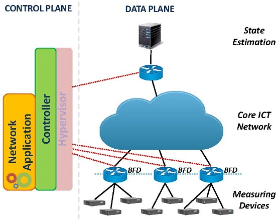
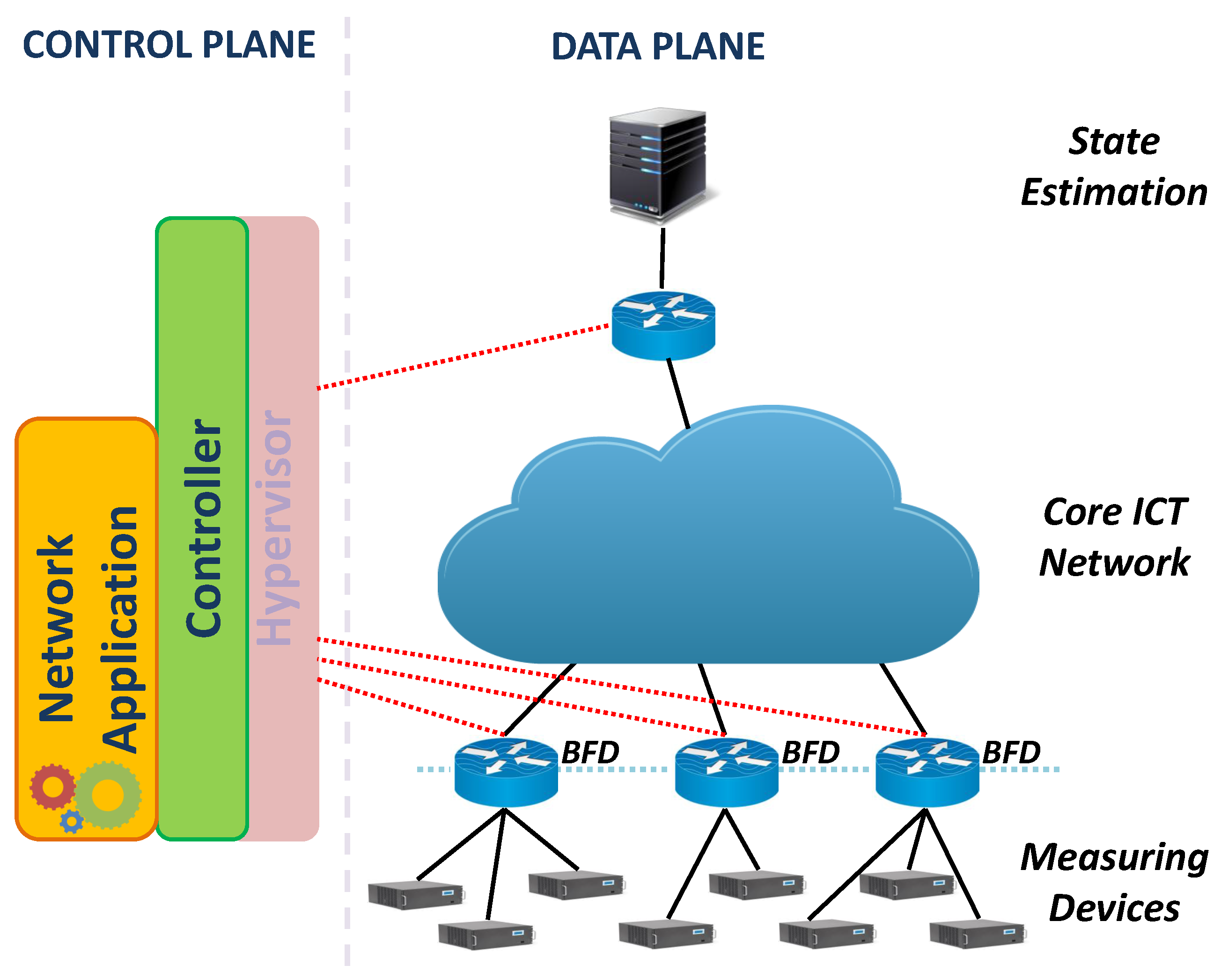
SDN rises from the need to overcome these limits. Figure 1 shows a generalized view of the SDN architecture. The lowest level, called data plane, is made of FDs specialized in managing the data traffic based on the forwarding rules installed by the SDN controller. The SDN controller translates requirements coming from network applications into control actions which are then distributed to FDs in the form of flow tables using so called southbound Application Programming Interface (API), of which Openflow is the most well-known and deployed [19,20] and it is also the one used in our test scenario. Each entry of a flow table has three parts: a matching rule, actions to be executed in case of matching, statistic counters for matching packets. Starting from OpenFlow Version 1.3, also a special kind of tables called meter tables have been introduced. Meter tables can be installed by the controller and be referenced by a flow rule, in order to meter quantities of the considered flow such as bitrate, packet rate or burst size and apply actions such as packet drop or Differentiated Services Code Point (DSCP) remark in the IP header for QoS packet classification purposes. Network Applications are the brain of the system and are responsible for coordinating the use of network resources according to the set goals. Thus, the role of the controller is to take as input the network application’s requirements and translate them into an FD understandable language (e.g., OpenFlow) in order to instruct the underlying data network. Examples of network applications are load balancing policies and network discovery protocols.
As to network resources’ availability, one of the characteristics of SDNs is the possibility to slice a single underlying physical network into many virtual (i.e., logical) networks which coexist thanks to a so called hypervisor, which allocates a slice of resources to any designated controller [21]. Many hypervisors have been developed in recent years [22]. Five slicing criteria are usually considered: bandwidth, topology, traffic, device CPU, and forwarding tables. Each network slice is managed by a controller which is allowed to act only on its own network slice. Thus, the same physical network infrastructure can be used for a mixture of applications logically independent. In our scenario, bandwidth constraints are supposed. This means that the available bandwidth for SE can either being considered as constrained by physical capacity limits of the links or by the logical link limits imposed by bandwidth virtual slicing of the hypervisor. In the latter case, the allocation of the resources could be changed (increased or decreased) dynamically by the hypervisor for the various slices. One of the case studies considered in the following takes into account such a case.
Other triggering events considered here are: the case in which a Measurement Device (MD) stops sending data, either unexpectedly or as a planned maintenance action, thus releasing its allocated resources; the case in which a new MD is installed. Either case, the data plane will communicate these changes to the control plane and the network application will be triggered in order to react promptly to these changes by reassigning network resources in an optimal manner. The next sections will detail on how these events are handled and how the optimization problem is formulated.
4. Considered System
Consider Figure 2 which represents the system under investigation and Table 1 which summarizes the symbols used. The electric network is populated by a set M of MDs with cardinality . Each MD is identified with the index m (belonging to the corresponding set of indexes) that send measurement packets about various points of the grid to a remote server estimating the state of the network. A generic has access to the core ICT network through a FD which functions as the gateway of the subnetwork. FDs placed between the access and the core network are identified with the index k and named Border Forwarding Devices (BFD). The totality of the BFDs constitute the set K while the set of MDs attached to form the set . Therefore
The bandwidth capacity allocated to for transmitting the aggregated data received from is indicated as
where is the bandwidth generated by . Let us consider the MDs to be PMUs and define and respectively as the maximum reporting frequency of the PMU and the granted reporting frequency, i.e., the number of measurement packets per second forwarded by the from to the state estimator. Moreover, for each PMU , where is the size in bytes of each packet. For the sake of simplicity, we consider to be equal for all PMUs in this system, so that and (the constraint on the packet rate at each ) differ just by a constant scale factor . These are the variables which will be used for the optimization of the accuracy. Nevertheless, the same optimization can be implemented considering as variables and as constraints. If
we say that a violation on the constraint of the reporting frequency of is present and thus a reduction (i.e., subsampling) of the reporting rate is necessary in order to let the ICT network work at its maximum without clogging.
However, some MDs such as PMUs, do not allow to change the reporting frequency at runtime and would require the operators to stop data flows to reconfigure the device. In addition, since data reported at a higher rate could serve for more than one application, it is inconvenient to set a priori the reporting frequency to a lower value. Indeed, the use of SDN would allow to create differentiated forwarding rules to serve more than one application at the same time using customized measurement reporting frequency.
The role of the network application is to optimize the resulting accuracy of the SE based on the knowledge of the considered electric network gathered from the MDs and on the knowledge of the constraints . The outcome of the accuracy Optimization Routine (OpR) consists of the values to be communicated to the various attached to using the control link shown in Figure 2 with a dashed line.
Overall, in the considered system, the controller is involved in the following runtime activities triggered by a new packet received (Figure 3):
- when the packet is received from a BFD because a data flow does not have a matching rule in its flow tables, the controller triggers a OpR passing the updated set of active MDs and waits for the updated values; then it sends a packet to the calling BFD in order to add a new meter and updates the value of all data flows already active; finally, it sends a message on new rules to be installed in the flow tables of all FDs from the MD to the data sink, in order to manage the new data flow;
- if a data flow has been idle for t seconds (the value of t is set in the design phase), a message is received from the BFD attached to the related MD to communicate that data flow has stopped; as a consequence, the controller triggers the OpR passing the updated set of active MDs and waits for the updated values; when received, it sends a message to the calling BFD in order to remove the meter associated to the expired data flow, updates the value of all data flows still active and removes the unnecessary forwarding rules from all the FDs involved;
- when a packet is received from either the hypervisor or the state estimator, concerning relevant changes of either the electric or the ICT network (e.g. MD’s degraded accuracy or allocated link’s bandwidth capacity), the controller triggers the OpR of the updated network values and then it sends a message to all BFDs involved, in order to update the meters’ value as a result of the updated optimization.
Before detailing into how these activities are implemented in a SDN, the next section discusses the formulation of the accuracy’s optimization problem which represents the network application considered.
5. Optimization’s Problem Formulation
The state estimation is the main application layer on which management and control systems of modern power network rely [23]. The SE gives a snapshot of the network operating conditions at a given time instant, by aggregating measurement data from the field along with any other available information on topology and breakers status, so that the grid can be safely operated. The SE gives knowledge about the status of the network in terms of node voltages, branch currents and power flows. It computes the quantities of interest in any node/branch of the network (in particular, the voltage profile) starting from electrical quantities measured with a given accuracy. For this reason, estimation results reflect the accuracy of measurements: the picture must be as accurate as possible since the accuracy of the estimation is decisive for SE-based decisions. Nowadays a great effort is ongoing to upgrade the monitoring infrastructure and measurement devices accuracy and, in particular, it is expected that PMU will play a crucial role in this perspective.
The SE can be formalized as an inverse problem. Its mathematical formulation depends on the relationship between measurements and state variables. For a detailed introduction to the SE paradigm and, in particular, to the estimation algorithms based on Weighted Least Squares (WLS), it is possible to refer to [23], while, for SE with PMU measurements, a thorough discussion is available in [24]. In the following, the principles are recalled and the aspects that link SE to the communication infrastructure are highlighted. The general measurement model adopted for SE can be represented as:
where: is the vector of the P measurements gathered from the network (from the devices) and of the chosen pseudo-measurements (knowledge obtained from a priori information exploited in case of a lack of sufficient number of MDs to make the system observable); is the vector of the measurement functions; is the vector of the N state variables; is the so-called measurement noise vector. is assumed to be composed of independent, zero mean random variables, with covariance matrix .
The state vector includes variables that are sufficient to derive all the other quantities of interest. Different formulations of the problem exist and efficient choices for are:
- node voltages (see, for instance, [23]): the state can be, for instance, represented in polar coordinates as ), where and are the amplitude and phase angle of the voltage of bus i and is the number of buses.
- branch currents plus a reference voltage (see, for instance, [25]): the state is typically adopted in rectangular coordinates as , where and are, respectively, the real and imaginary parts of the current phasor at branch l, is the phasor of the voltage assumed as a reference, and is the number of network branches.
The above presented expressions are referred to a single phase of the network for the sake of brevity and clearness of notation, but it should be recalled that SE typically requires a three-phase formulation. The measurements can generally include voltage and current amplitude measurements, synchronized phasor measurements from PMUs, active and reactive power measurements. Depending on the different measurement types and state formulations, the measurement functions in can be non-linear.
Different methods are available in the literature for solving the SE (see [24]). Here, a WLS approach is used and briefly explained for the sake of completeness. In the WLS-based approach, the state is estimated iteratively by means of linear system solution. In particular, the so-called normal equations are solved at each iteration to update the state vector computation as:
where is the state vector at iteration n. The stop condition for the algorithm convergence is given by , with an assumed small tolerance value , meaning that no further updates of the state vector are needed.
is the Jacobian containing the derivatives of the measurement functions with respect to the state variables and is the weighting matrix, chosen as the inverse of the covariance matrix .
is the so-called Gain matrix while its inverse, namely the covariance matrix of the estimated state vector [23] is the objective function to be minimized:
If the weighting matrix can be expressed as diagonal matrix
the uncertainty matrix can be expressed as
where is the ith row of the Jacobian matrix and is, in general, a function of the estimated state.
In this paper, measurements from PMUs are considered and (10) is exploited, by adapting it to the case of synchronized measurements obtained from PMUs at different reporting frequencies. With such an assumption, it is possible to express the measurement functions linearly [24], when the state is expressed in rectangular coordinates as , as assumed in the following. In fact, the PMU voltage phasor measurement at node j corresponds to direct measurements of the real and imaginary parts of , while the PMU current measurement at a branch l, represented by the couple of nodes , that is by its start and end nodes, can be written as:
that can be translated in the real and imaginary components:
It is there clear that the is constant and the solution of the state estimation can be performed in one WLS estimation step. The gain matrix (7) can be expressed, under the aforementioned assumptions, as a sum of matrices, each corresponding to a PMU set of measurements, as follows:
where is the weighting matrix corresponding to all the measurements from the ith PMU (all measured voltage and current phasors in rectangular coordinates) and is the submatrix corresponding to the same measurements subset.
In this paper, it is proposed to perform the SE at regular intervals (for instance, once per second), exploiting the measurement capability of PMUs. Since PMUs can work at higher reporting rates, the average of each measured quantity is used for the SE and chosen as input for the SE routine. This is an approach that can be adopted in SE estimation when high PMU reporting rates are used and also when PMU data are mixed with data from different measurement sources. The state of a power network is slowly varying with respect to the assumed SE timescale and thus the final measurement accuracy can benefit from the higher PMU data rate. It is thus proposed to use a decreasing monotonic function of the measurement rate when defining the accuracy of each PMU measurement used in SE, and consequently its weight in the WLS. For each measurement i from (that is ) the uncertainty of the average of measurements collected in a second is considered in the following. The covariance thus becomes and the weighting matrix updates as follows:
and
becomes the Gain matrix of the SE and is a function of values, that is of the PMU reporting frequencies. The covariance matrix is also a function of the reporting frequencies, and thus is linked to the bandwidth required by each PMU stream. Equation (16) can thus become the mean to optimize the accuracy of the estimator imposing the communication requirements and plays a key role in the definition of proposed objective function.
In fact, the objective function of the optimization process introduced in this paper has to reflect the overall estimation accuracy of the SE when the data flows from BFDs and MDs are subject to constraints. For this reason, it is possible to assume:
where is the vector of reporting frequencies, the dependence of the covariance matrix on the rates is made explicit and indicates the trace of the matrix. The optimization is thus conceived as the minimization of the trace of the covariance matrix (sum of the variances of the estimation errors of all the estimated quantities) depending on the set of reporting frequencies of PMUs.
As in [26], it is possible to express the optimization as a convex optimization problem by means of relaxation. By relaxing the integer property of the reporting frequencies, it is possible to write the optimization problem as an A-optimal experimental design problem, as follows:
where and define the communication constraint associated to the kth BFD, while is the cardinality of the set K. It is important to underline that each reporting frequency has lower limit 1, because observability must be guaranteed. If observability holds, such limit can be removed, thus imposing only .
As mentioned in Section 4, the communication constraints for the optimization are given by the packet rate constraints for each PMU data flow and by the reporting frequency limits. They can be expressed as
and thus , is the indicator vector of the PMU set corresponding to the kth BFD.
For the solution of the optimization, the problem (18) can be translated into a semidefinite programming (SDP) problem as follows [27]:
where is the vector of auxiliary variables, is the -size vector of ones and is the kth vector of the canonical basis. Given the optimal vector as output of the optimization process, the vector can be used to represent the set of reporting frequencies that minimizes the estimation uncertainty, expressed in terms of the sum of the covariances of state variables.
As recalled above, the state variables are the real and imaginary parts of the voltage phasors at each node of the network. In practice, the estimated voltage amplitude and phase angle (magnitude and angle of the corresponding complex phasor) at each node are required. Such estimations are obtained by the corresponding transformation. In terms of uncertainty, it is possible to transform also the covariance matrix , using the first order expansion and the law of uncertainty propagation in [28]. When an electric network is considered, the voltage amplitudes are expressed in per units with respect to the base voltage. They are thus closed to one and, since the estimation uncertainty is small, it is possible to consider, in a first order approximation, the transformation from rectangular to polar coordinates at each node as a simple rotation. For this reason, the trace of the covariance matrix is preserved and can be used to configure the data stream to minimize the impact of measurement uncertainty on voltage amplitude and phase angle profiles.
6. System Implementation
The considered system has been implemented using Mininet [29], a network emulator which creates a network of virtual hosts, switches (in the context of SDN, the term switch is equal to the term Forwarding Device used so far, rather than that of a classic level 2 networking device), controllers, and links hosted in a standard Linux OS. For this study, a machine with 2 GB RAM and a dual-core 2 GHz processor running Ubuntu 12.04 have been used. OpenFlow [20] has been chosen as communication protocol between the switches on the data plane and the controller. In particular, version 1.3 is used, since previous versions do not define the use of meter tables. Concerning the virtual switches used, ofsoftswitch13 [30,31] has been chosen. As matter of fact, while Open vSwitch [32,33] is usually employed in the Mininet environment, meter tables are an optional feature and to date, ofsoftswitch13 is the only virtual switch implementing this feature together with some commercial hardware switches.
In the control plane, for similar reasons of compatibility with OpenFlow version 1.3, a Ryu Controller [34] has been used. Ryu Controller is an open SDN Controller supported by Nippon Telegraph and Telephone Corporation providing software components in Python language, with well-defined APIs, that make it easy to develop new network management and control applications. For the sake of simplicity, a hypervisor has not been implemented (since the considered scenario deals only with a potential logical slice of the physical network which is used for State Estimation) and potential changes for the bandwidth allocated to a FD are artificially passed to the controller using the available APIs.
Each Mininet host connected to a BFD is a Linux-based host that can be seen as a stand-alone machine running its own tasks. In order to simulate the behaviour of a real PMU, in our case each Mininet host reads pre-stored data about the monitored node of the electric network and build the PMU packet according to the IEEE C37.118.2-2011 Standard for Synchrophasor Data Transfer [35]. The standard defines the possibility to use either Transmission Control Protocol (TCP) or User Datagram Protocol (UDP) at the transport level. Since in the envisioned scenario, the BFDs selectively drop part of the packets according to the meter table installed, the use of UDP is the only viable solution.
Finally, the network application has been implemented in Python, using the RYU APIs to communicate with the controller. In addition, the OpR developed leverages on the CVXOPT solver library [36] to implement the solution to the customized SDP problem formulated in (20).
Software Defined Network Data Flow Management at Runtime
Upon session establishment, the controller sends a FeaturesRequest message to all the FDs connected to it. Every FD responds with a FeaturesReply message which is handled by the Ryu controller. The messages and their structure as well as the library functions described in the followings can be found at [37]. Typically, in this phase, the controller also installs the first rule in the FD flow table using the OFPFlowMod instruction. This rule tells the FD to forward to the controller using the wildcard any packet received which does not match any of the other rules installed (see function in [37]).
Consider Figure 4, which represents the lifecycle of a data flow using a state diagram where the state is the combination of the flow state for the considered and the state of the OpR when the data flow from is included in the optimization: both can be either idle or active. Table 2 lists the events that characterize a change of state. When a new data flow enters the BFD attached to the source , the packet is forwarded to the controller. The role of the controller is to handle the received packet and learn the address of the host attached to the BFD from the source address field, in order to install forwarding rules to route the packets to the intended destination. Additionally, the controller forwards the content of the UDP packet to the network application, which takes into account the new device and its declared accuracy and runs the OpR taking into account the packet rate constraints at each BFD.
Once the OpR has been completed, the network application triggers the controller to install a new meter in the BFD attached to the new MD generating the data flow as well as to update the set packet rate for all MDs with a flow already active. Active data flow means that a certain data flow is received by the SE. To do so, the OFPMeterMod of the ryu.ofproto library [37] is used, setting the meter to compute the packet rate with the flag OFPMF_PKTPS and passing as type of control the instruction OFPMeterBandDrop with paratemer “rate” which indicates the maximum rate achievable in packets per second parsed by the OpR. In addition, a new rule is installed in the flow table of the calling BFD using the OFPFlowMod instruction which: tells the BFD where the flow should be forwarded; binds the flow to the installed meter; sets an idle_timeout value, which tells the BFD to notify the controller if that data flow has been inactive for more than idle_timeout seconds.
From this moment on, the flow is active and the SE will receive data from the newly installed MD without these packets being forwarded to the control plane. As long as the flow remains active, the only change that will take place for the considered data flow is an update of the rate value based on the following events: a new MD is installed or an idle MD is removed; the hypervisor communicates a change in the allocated bandwidth for at least one of the BFDs; a new OpR is triggered by the SE. As a matter of fact, apart from communicating the data which are necessary for the accuracy optimization at regular intervals, the SE sends a message to the controller using the OFPP_CONTROLLER wildcard in the address field to trigger a new OpR in the following cases: the accuracy of one of the PMUs has changed; the state of the electric grid is not steady; the system has been configured to run a new accuracy optimization at regular intervals.
When a MD stops sending packets to the SE either for maintenance purposes or as an unexpected behaviour, the controller is notified by the BFD attached to the MD after idle_timeout seconds, which automatically runs a new accuracy OpR, updates the rate of all the meter tables binded to active flows, and removes the meter table and the flow table rules concerning the idle MD from all interested FDs. To do so, the flag value for the meter and the flag value for the flow rules are set in the relative instruction. This represents a relevant step forward with regard to the current management of a smart grid-related ICT network, since these changes take place without requiring any manual intervention and reconfiguration from a network operator.
7. Test Case and Results
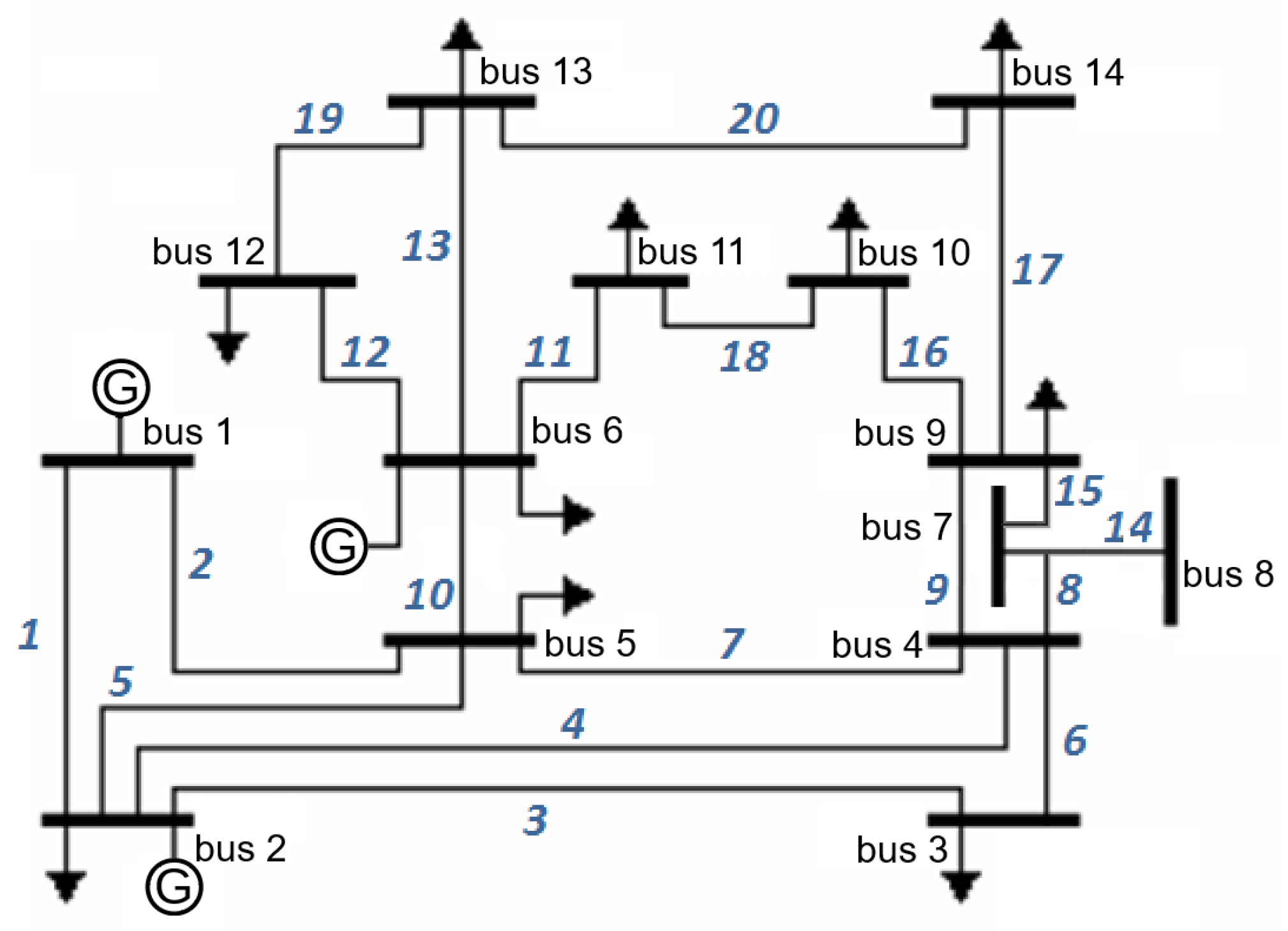
In this paper, the IEEE 14-bus network is used to verify the validity of the proposed approach. Such network represents a portion of the American Electric Power System (in the Midwestern US). It has 14 buses, 5 generators, and 11 loads. The numbers identifying all the network buses and branches are shown in Figure 5.
More details about the test case data are available in [38], where, in particular, the line parameters (resistance, reactance and shunt susceptance of the -model for each branch), along with information about loads and generators, are given. Starting from the available nominal data of power consumption and generation, the reference values for the main quantities of interest, that is the magnitudes and angles of the voltage phasors at each node of the network, have been computed, performing a power-flow, and used for all the tests. In this way, all the voltage and branch currents phasors are evaluated and can be used as reference values for PMU measurements. To define a meaningful measurement system, the observability of the system is guaranteed by using a minimum set of PMUs at nodes 2, 6, 7, 9 found by adopting the simple optimal placement method for observability in [39]. In addition, node 13 is monitored in the scenario (see Section 7.3) in which five PMUs are present. We suppose PMUs at nodes 2 and 6 to be attached to the same . Similarly, the PMUs at nodes 7, 9 and 13 are attached to . For the sake of simplicity, we assume the index m of the MD to be equal to the node where the PMU is installed and thus each PMU is directly referred to by means of its associated node index. Each PMU measures the voltage phasor at the installation node and all the current phasors of outgoing branches. Such configuration is set without loss of generality, because it is possible to choose every alternative measurement system, given that the observability constraint is satisfied. Obviously, different PMU systems can comply with different placement constraints, but the considerations in the following have general validity.
7.1. Optimization Algorithm’s Results
In a preliminary test with four PMUs, the accuracy values associated to PMUs 6, 7, 9 are considered to be and ( corresponds to and is typically used to express PMU phase angle uncertainty) for voltage amplitude and phase angle measurements, respectively, while PMU 2 has accuracies and . The measurement errors are considered as Gaussian variables with a coverage factor of 3 (the standard uncertainty is one third of the absolute accuracy). The idea is to show a scenario where the PMUs can have different accuracies, as in a real scenario, where PMUs are from different vendors, with different specifications, and/or different configurations. All the PMU can operate at the maximum reporting frequency suggested by [35] that are nowadays typical for commercial PMUs.
The amount of data generated by a PMU depends, among other aspects, on the number of channels, the device configuration, and the encapsulation protocol. For instance, with a TCP/IP packetization (in [35] a 44-byte header is, for instance, considered) for 3 three-phase measurement channels and reported sequences, the packet size (see Section 4) is 214 bytes when floating-point format is used. Such packet size does not include the other analog and digital data that can be included in practice (see [35] for details).
As a first result, Figure 6 shows an index of the average uncertainty among all the network nodes for the voltage amplitude estimations as a function of the bandwidth constraint, both in the case of equally partitioned among the participating and in the case in which the developed optimization algorithm is applied. In details, the following index is used:
where is the estimation standard deviation associated to the voltage amplitude estimation at node i. Since is in per unit, is expressed in percentage with respect to the base voltage and the coverage factor 3 is chosen according to the assumption made for the definition of the measurement errors, in order to represent an expanded uncertainty value. Table 3 shows the reporting frequency configurations corresponding to fair and optimized partitions of Figure 6.
The estimation accuracy generally worsens as the overall available packet rate is reduced, but the packet rate allocation between the two BFDs is essential to enhance the estimation accuracy. The results show how the lack of optimization can lead, in this specific case, to an increase of more than in the average uncertainty of the voltage amplitude estimations. When the optimization is performed, the rate of the most accurate PMU is typically privileged by the associated BFD, as expected, but the optimization operates at a global level, thus keeping into account the influences among the MDs, given the assumed constraints. Similar results and considerations hold also for voltage phase angle estimations, but are not reported here for the sake of brevity.
7.2. Test Case 1: Change of at the BFDs
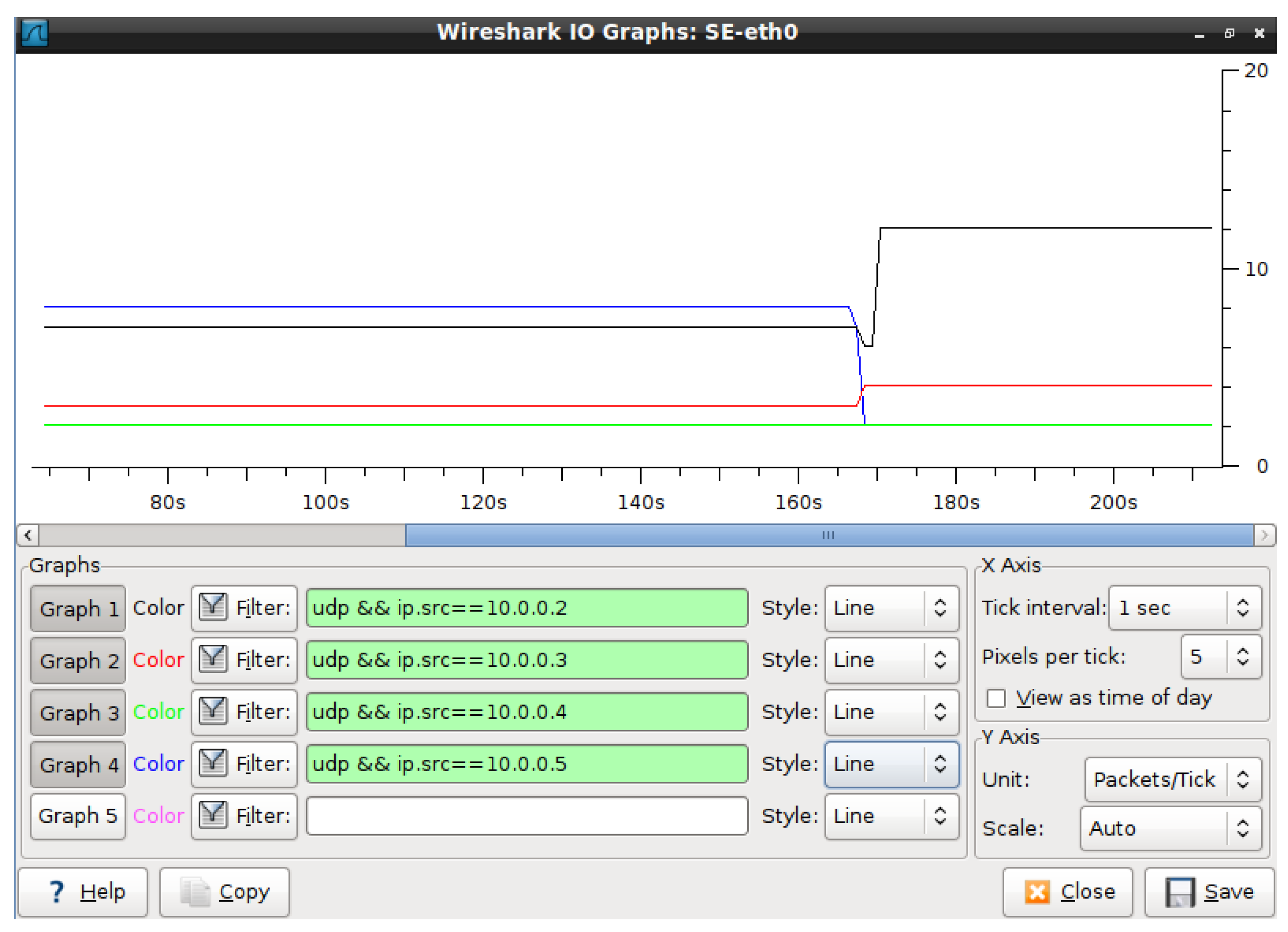
Consider Figure 7, which represents the packet rates received by the SE and captured by wireshark for the case of all PMUs with accuracy and for voltage amplitude and phase angle measurements. Initially, the constraints are . For these constraints, the network application outputs the following values: , , , . However, at second 167, the allocated bandwidth for the BFDs is changed and the constraints become . Thus, a new optimization is triggered, resulting in the following values: , , , . It can be seen that after the bandwidth change, the additional communication budget available on is split between the two PMU in in a similar way with respect to initial proportions, while keeping into account the reduced impact of the PMUs 7 and 9 on the overall accuracy. The estimation accuracy is slightly enhanced, as reported in Table 4, thus showing how the considered PMU subsets are strongly related in the case at hand.
When PMU 2 has higher accuracy ( and ), a change in the between the two BFDs, shows a more variegate behavior (Table 5). If the hypervisor changes the allocated bandwidth for the BFDs to the optimization allows a greater contribution from PMU 2 and thus a reduction greater than occurs, whereas if BFDs constraints switch in the opposite way to , the performance are strongly affected. In fact, in the latter case, the constraint change results in an increase of + in the expanded uncertainty with respect to the previous case and about + with respect to the case with equal bandwidth.
7.3. Test Case 2: Change of the Set M of MDs
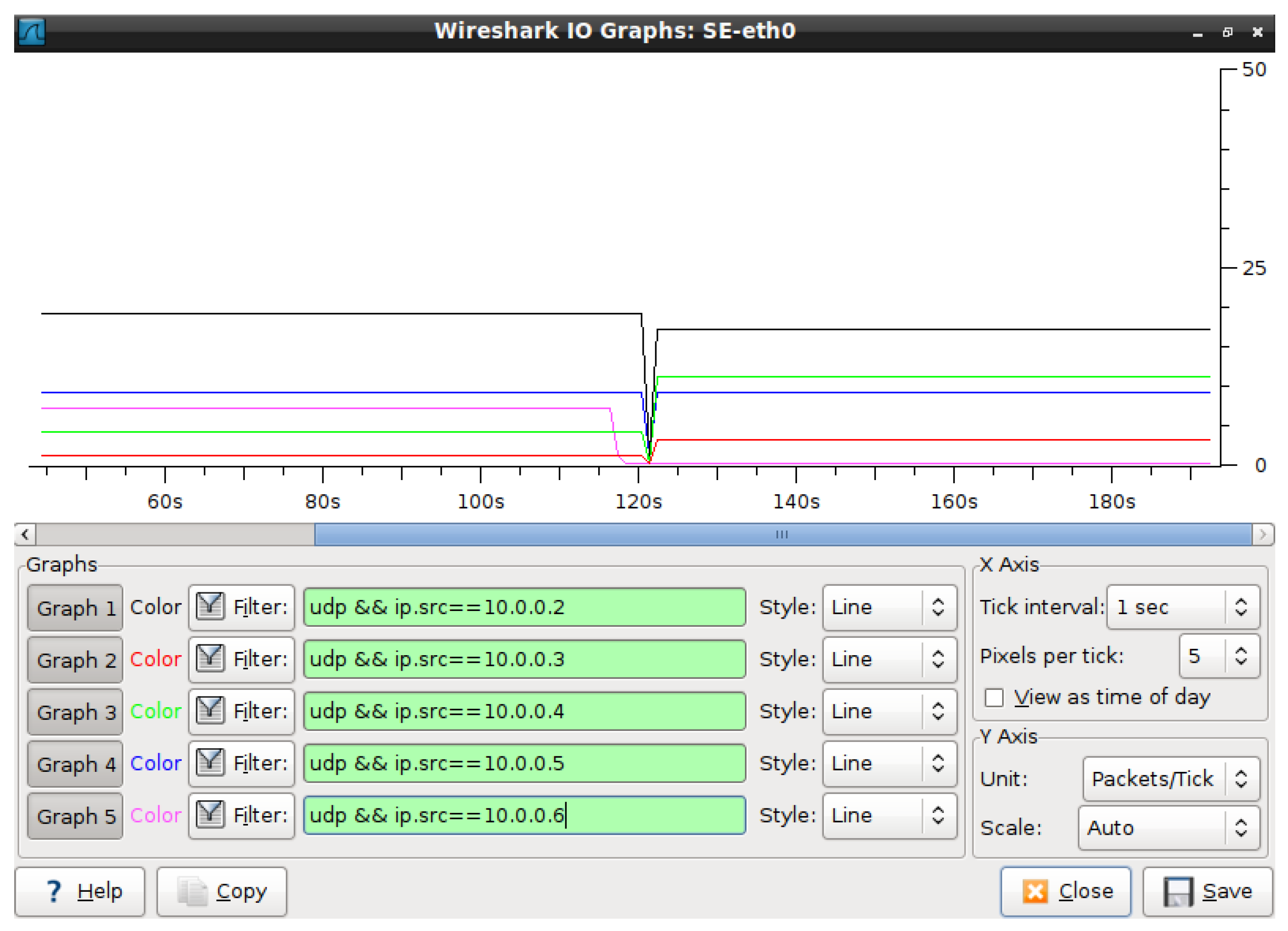
In the second test case, similarly to the first one, five PMUs are present with accuracy and for voltage amplitude and phase angle measurements, respectively. Consider Figure 8. The constraints for the two BFDs are . For these constraints, the network application outputs the following values: , for the PMUs connected to ; , , for the PMUs connected to . In our test case, the PMU at node 13 stops working at second 117. However, since the is set to 3 seconds, it can be noticed that a new optimization is triggered only at second 120, resulting in the subsequent change of the following values: , for ; , for . This can be seen in Figure 7. It is important to recall that the available resources, in terms of communication constraints, are the same before and after the event. The new optimization tries to redistribute the uncertainty budget among the remaining PMUs. For this reason, the PMU in node 6, which partially overlaps with the PMU in node 13 in terms of measured quantities, gets a higher rate to compensate the loss of information. In Table 6, the average uncertainties before and after PMU removal are reported and it is possible to note that the estimation performance is basically maintained thanks to the global reorganization.
It is interesting to higlight how such test case can also explain what happens in the presence of bad data in PMU measurements. Bad data detection and removal capability are strongly related to PMU pre-processing and to SE elaboration modules. Bad data can be, for instance, detected by the classic Chi-square test (see [23] for further details) and removed re-executing the SE routines at application level in the control center (Figure 2). When data from a given PMU are identified as a affected by gross errors, the state estimator informs the controller that considers the PMU as virtually disconnected and triggers the OpR updating the set of active MDs. The controller then sends messages to the BFDs to update values. The BFD associated to the PMU marked as bad data source is in charge of reducing its frequency to a very low rate that does not affect the communication bandwidth. If PMU 13 is undergoing problems, the results are identical to the previous test case. On the contrary, when bad data is limited to a few measurements in a data flow, it is easier to exclude them from the estimator, without altering the communication flows. The state estimation accuracy is only temporary reduced depending on the discarded measurements during the refresh time interval. For example, in previous configuration, if a single bad data is found for PMU 13, the average unceratainty of voltage amplitude becomes times higher ( if ). As above said, this is a temporary condition: if the problem persists, the optimization is triggered as described.
8. Conclusions
In this paper, the use of Software Defined Networks in the context of measurement systems for state estimation based on synchronized measurements has been presented. The goal has been to implement a strategy leveraging on the capabilities of Software Defined Networks, to optimize the accuracy of the state estimation based on the available bandwidth resources and on the knowledge of the uncertainty of the measurement devices. The results have demonstrated the potential in using an approach with Software Defined Networks to adapt promptly to changes that can occur in the electric or the telecommunications network without the need of manual intervention to update the measurement system.
As to the development of the network application, we demonstrated the advantage in assigning a different measurement reporting rate to any involved PMU, depending on the goal of the system (i.e., accuracy) and taking into account the actual importance of the measurements coming from a monitored node.
It should be noticed that the use of Software Defined Networks allows to skim the rates of the data flows in order to operate efficiently the network. Nevertheless, this process does not take directly into account the actual content (i.e., measurement) of each packet at forwarding device level and could result in the loss of insightful information in some special cases. A complementary approach, as the one presented in [40], would be to take decisions as to whether to send a measurement or not, based also on the checking of the actual measurement’s content. While current flow tables in Software Defined Networks only analyze the header of the packets, it cannot be excluded that in the future the same approach will be available for the payload, thus further boosting the convenience in using this paradigm for Smart Grid applications.
Acknowledgments
This work has been supported by Regione Autonoma della Sardegna, L.R. 7/2007: “Promozione della ricerca scientifica e dell’innovazione tecnologica in Sardegna, annualità 2012, CRP-60511”.
Author Contributions
Alessio Meloni and Paolo Attilio Pegoraro conceived the idea of exploiting sinergies between the communication and measurement infrastructures. Alessio Meloni formulated the communication problem based on SDN and implemented the infrastructure and the simulations. Paolo Attilio Pegoraro formulated the measurement problem and implemented the corresponding algorithms. Luigi Atzori contributed to the implementation of the SDN infrastructure and the overall technical revision of the paper. Sara Sulis conceived the network scenario for the test cases and contributed to the interpretation of the results.
Conflicts of Interest
The authors declare no conflict of interest.
List of Acronyms
| API | Application Programming Interface |
| BFD | Border Forwarding Device |
| DSCP | Differentiated Services Code Point |
| FD | Forwarding Device |
| IED | Intelligent Electronic Device |
| IoT | Internet of Things |
| M2M | Machine-to-Machine |
| MD | Measurement Device |
| OpR | Optimization Routine |
| PMU | Phasor Measurement Unit |
| QoS | Quality of Service |
| SCADA | Supervisory Control and Data Acquisition |
| SDN | Software Defined Network |
| SDP | Semidefinite Programming |
| SE | State Estimation |
| SG | Smart Grid |
| SM | Smart Meter |
| TCP | Transmission Control Protocol |
| UDP | User Datagram Protocol |
| WAMS | Wide Area Monitoring Systems |
| WLS | Weighted Least Squares |
References
- Gupta, A.; Jha, R.K. A Survey of 5G Network: Architecture and Emerging Technologies. IEEE Access 2015, 3, 1206–1232. [Google Scholar] [CrossRef]
- Ardito, L.; Procaccianti, G.; Menga, G.; Morisio, M. Smart Grid Technologies in Europe: An Overview. Energies 2013, 6, 251–281. [Google Scholar] [CrossRef]
- Shin, I.J.; Song, B.K.; Eom, D.S. International Electronical Committee (IEC) 61850 Mapping with Constrained Application Protocol (CoAP) in Smart Grids Based European Telecommunications Standard Institute Machine-to-Machine (M2M) Environment. Energies 2017, 10, 393. [Google Scholar] [CrossRef]
- IEEE Std C37.118.1-2011 IEEE Standard for Synchrophasor Measurements for Power Systems; Revision of IEEE Std C37.118-2005; IEEE: Piscataway, NJ, USA, 2011; pp. 1–53.
- Meloni, A.; Atzori, L. The Role of Satellite Communications in the Smart Grid. IEEE Wirel. Commun. 2017, 24, 50–56. [Google Scholar] [CrossRef]
- Erol-Kantarci, M.; Mouftah, H.T. Energy-Efficient Information and Communication Infrastructures in the Smart Grid: A Survey on Interactions and Open Issues. IEEE Commun. Surv. Tutor. 2015, 17, 179–197. [Google Scholar] [CrossRef]
- Thompson, J.; Ge, X.; Wu, H.C.; Irmer, R.; Jiang, H.; Fettweis, G.; Alamouti, S. 5G wireless communication systems: Prospects and challenges [Guest Editorial]. IEEE Commun. Mag. 2014, 52, 62–64. [Google Scholar] [CrossRef]
- Boccardi, F.; Heath, R.W.; Lozano, A.; Marzetta, T.L.; Popovski, P. Five disruptive technology directions for 5G. IEEE Commun. Mag. 2014, 52, 74–80. [Google Scholar] [CrossRef]
- Zhang, J.; Seet, B.C.; Lie, T.T.; Foh, C.H. Opportunities for Software-Defined Networking in Smart Grid. In Proceedings of the 2013 9th International Conference on Information, Communications and Signal Processing, Tainan, Taiwan, 10–13 December 2013. [Google Scholar]
- Kim, J.; Filali, F.; Ko, Y.B. Trends and Potentials of the Smart Grid Infrastructure: From ICT Sub-System to SDN-Enabled Smart Grid Architecture. Appl. Sci. 2015, 5, 706. [Google Scholar] [CrossRef]
- Kreutz, D.; Ramos, F.M.V.; Veríssimo, P.E.; Rothenberg, C.E.; Azodolmolky, S.; Uhlig, S. Software-Defined Networking: A Comprehensive Survey. Proc. IEEE 2015, 103, 14–76. [Google Scholar] [CrossRef]
- Narayanan, R.; Xu, K.; Wang, K.C.; Venayagamoorthy, G.K. An information infrastructure framework for smart grids leveraging SDN and cloud. In Proceedings of the 2016 Clemson University Power Systems Conference (PSC), Clemson, SC, USA, 8–11 March 2016. [Google Scholar]
- Cahn, A.; Hoyos, J.; Hulse, M.; Keller, E. Software-defined energy communication networks: From substation automation to future smart grids. In Proceedings of the 2013 IEEE International Conference on Smart Grid Communications (SmartGridComm), Vancouver, BC, Canada, 21–24 October 2013; pp. 558–563. [Google Scholar]
- Molina, E.; Jacob, E.; Matias, J.; Moreira, N.; Astarloa, A. Using Software Defined Networking to manage and control {IEC} 61850-based systems. Comput. Electr. Eng. 2015, 43, 142–154. [Google Scholar] [CrossRef]
- Goodney, A.; Kumar, S.; Ravi, A.; Cho, Y.H. Efficient PMU networking with software defined networks. In Proceedings of the 2013 IEEE International Conference on Smart Grid Communications (SmartGridComm), Vancouver, BC, Canada, 21–24 October 2013; pp. 378–383. [Google Scholar]
- Dorsch, N.; Kurtz, F.; Georg, H.; Hägerling, C.; Wietfeld, C. Software-defined networking for Smart Grid communications: Applications, challenges and advantages. In Proceedings of the 2014 IEEE International Conference on Smart Grid Communications (SmartGridComm), Venice, Italy, 3–6 November 2014; pp. 422–427. [Google Scholar]
- IEC TC57. IEC 61850: Communication Networks and Systems for Power Utility Automation; International Electrotechnical Commission: Geneva, Switzerland, 2010. [Google Scholar]
- Aydeger, A.; Akkaya, K.; Cintuglu, M.H.; Uluagac, A.S.; Mohammed, O. Software defined networking for resilient communications in Smart Grid active distribution networks. In Proceedings of the 2016 IEEE International Conference on Communications (ICC), Kuala Lumpur, Malaysia, 22–27 May 2016. [Google Scholar]
- McKeown, N.; Anderson, T.; Balakrishnan, H.; Parulkar, G.; Peterson, L.; Rexford, J.; Shenker, S.; Turner, J. OpenFlow: Enabling Innovation in Campus Networks. SIGCOMM Comput. Commun. Rev. 2008, 38, 69–74. [Google Scholar] [CrossRef]
- Open Networking Foundation. Available online: https://www.opennetworking.org/ (accessed on 25 March 2017).
- Chowdhury, N.M.K.; Boutaba, R. A survey of network virtualization. Comput. Netw. 2010, 54, 862–876. [Google Scholar] [CrossRef]
- Blenk, A.; Basta, A.; Reisslein, M.; Kellerer, W. Survey on Network Virtualization Hypervisors for Software Defined Networking. IEEE Commun. Surv. Tutor. 2016, 18, 655–685. [Google Scholar] [CrossRef]
- Abur, A.; Expòsito, A.G. Power System State Estimation. Theory and Implementation; Marcel Dekker: New York, NY, USA, 2004. [Google Scholar]
- Ponci, F.; Sulis, S.; Pau, M.; Angioni, A.; Pegoraro, P.A. State Estimation and PMUs. In Phasor Measurement Units and Wide Area Monitoring Systems, 1st ed.; Monti, A., Muscas, C., Ponci, F., Eds.; Elsevier, Academic Press: Cambridge, MA, USA, 2016; Chapter 6. [Google Scholar]
- Pau, M.; Pegoraro, P.A.; Sulis, S. Efficient Branch-Current-Based Distribution System State Estimation Including Synchronized Measurements. IEEE Trans. Instrum. Meas. 2013, 62, 2419–2429. [Google Scholar] [CrossRef]
- Kekatos, V.; Giannakis, G.B.; Wollenberg, B. Optimal Placement of Phasor Measurement Units via Convex Relaxation. IEEE Trans. Power Syst. 2012, 27, 1521–1530. [Google Scholar] [CrossRef]
- Boyd, S.; Vandenberghe, L. Convex Optimization; Cambridge University Press: Cambridge, UK, 2004. [Google Scholar]
- Bureau International des Poids et Mesures. Evaluation of Measurement Data—Guide to the Expression of Uncertainty in Measurement. Joint Committee for Guides in Metrology. 2008. Available online: http://www.bipm.org/en/publications/guides/gum.html (accessed on 25 March 2017).
- Mininet: An Instant Virtual Network on Your Laptop. Available online: https://www.mininet.org/ (accessed on 25 March 2017).
- Ofsoftswitch Project. Available online: http://cpqd.github.io/ofsoftswitch13/ (accessed on 25 March 2017).
- Fernandes, E.L.; Rothenberg, C.E. OpenFlow 1.3 software switch. In Salao de Ferramentas do XXXII Simpósio Brasileiro de Redes de Computadores e Sistemas Distribuıdos SBRC; UFSC: Florianópolis, Brazil, 2014; pp. 1021–1028. [Google Scholar]
- Open vSwitch. Available online: http://openvswitch.org/ (accessed on 25 March 2017).
- Pfaff, B.; Pettit, J.; Koponen, T.; Jackson, E.J.; Zhou, A.; Rajahalme, J.; Gross, J.; Wang, A.; Stringer, J.; Shelar, P.; et al. The Design and Implementation of Open vSwitch. In Proceedings of the 12th USENIX Symposium on Networked Systems Design and Implementation, Oakland, CA, USA, 4–6 May 2015; pp. 117–130. [Google Scholar]
- Nippon Telegraph and Telephone Corporation. Available online: http://osrg.github.com/ryu/ (accessed on 25 March 2017).
- IEEE Std C37.118.2-2011 IEEE Standard for Synchrophasor Data Transfer for Power Systems; Revision of IEEE Std C37.118-2005; IEEE: Piscataway, NJ, USA, 2011; pp. 1–53.
- CVXOPT. Available online: http://cvxopt.org/ (accessed on 25 March 2017).
- OpenFlow v1.3 Protocol API Reference for the Ryu Controller. Available online: http://ryu.readthedocs.io/en/latest/ofproto_v1_3_ref.html (accessed on 25 March 2017).
- Power Systems Test Case Archive. Available online: https://www2.ee.washington.edu/research/pstca/pf14/pg_tca14bus.htm (accessed on 25 March 2017).
- Xu, B.; Abur, A. Optimal Placement of Phasor Measurement Units for State Estimation; Final Project Report; PSERC: Tempe, AZ, USA, 2005. [Google Scholar]
- Pegoraro, P.A.; Meloni, A.; Atzori, L.; Castello, P.; Sulis, S. PMU-Based Distribution System State Estimation with Adaptive Accuracy Exploiting Local Decision Metrics and IoT Paradigm. IEEE Trans. Instrum. Meas. 2017, 66, 704–714. [Google Scholar] [CrossRef]
Figure 1.
Simplified view of an SDN architecture [11]. Solid lines represent data links. Dashed lines represent links between the controller and the FDs.
Figure 1.
Simplified view of an SDN architecture [11]. Solid lines represent data links. Dashed lines represent links between the controller and the FDs.
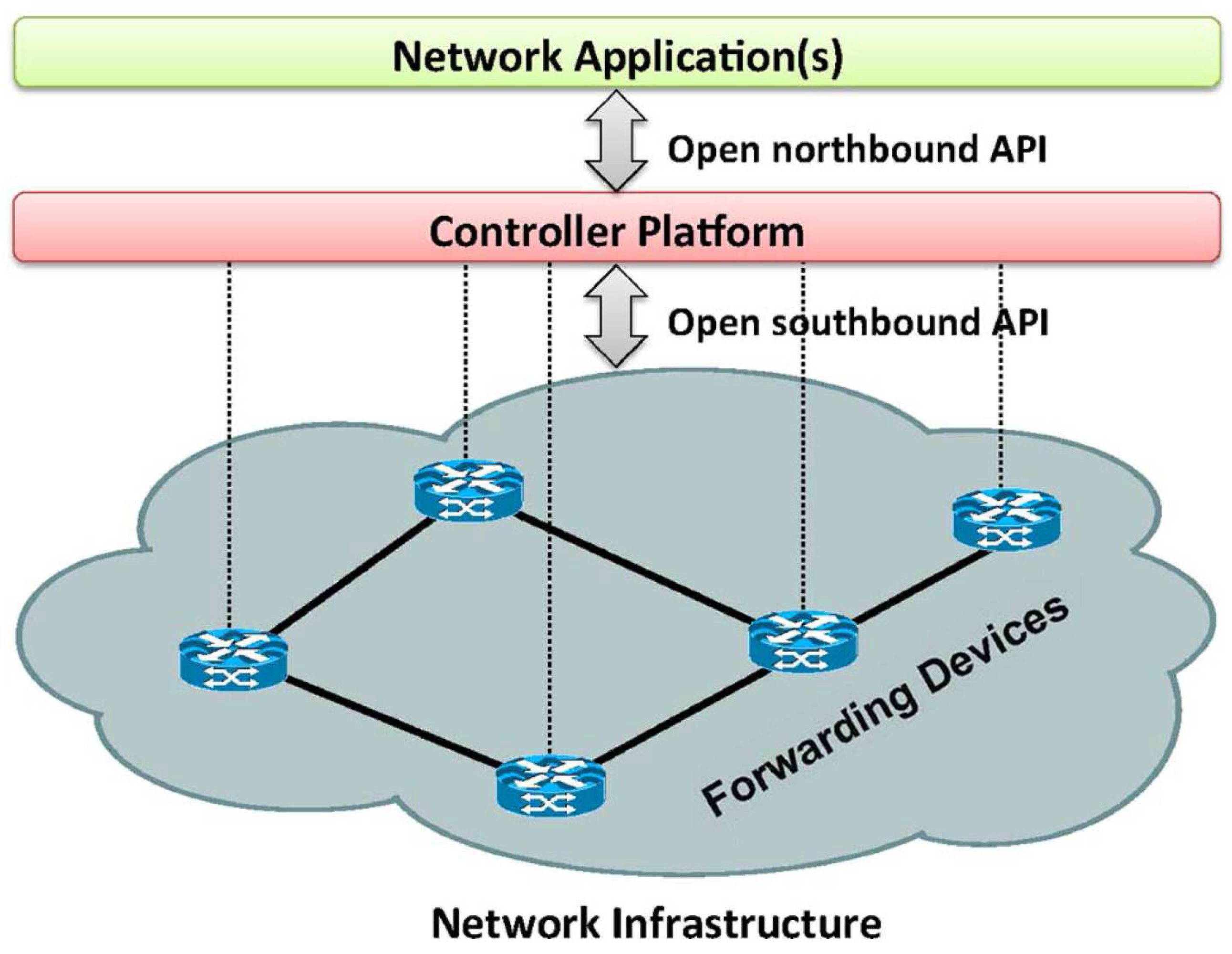
Figure 2.
Considered system. Solid lines represent data links. Dashed lines represent links between the controller and the FDs.
Figure 2.
Considered system. Solid lines represent data links. Dashed lines represent links between the controller and the FDs.

Figure 3.
Flowchart indicating controller’s activities.
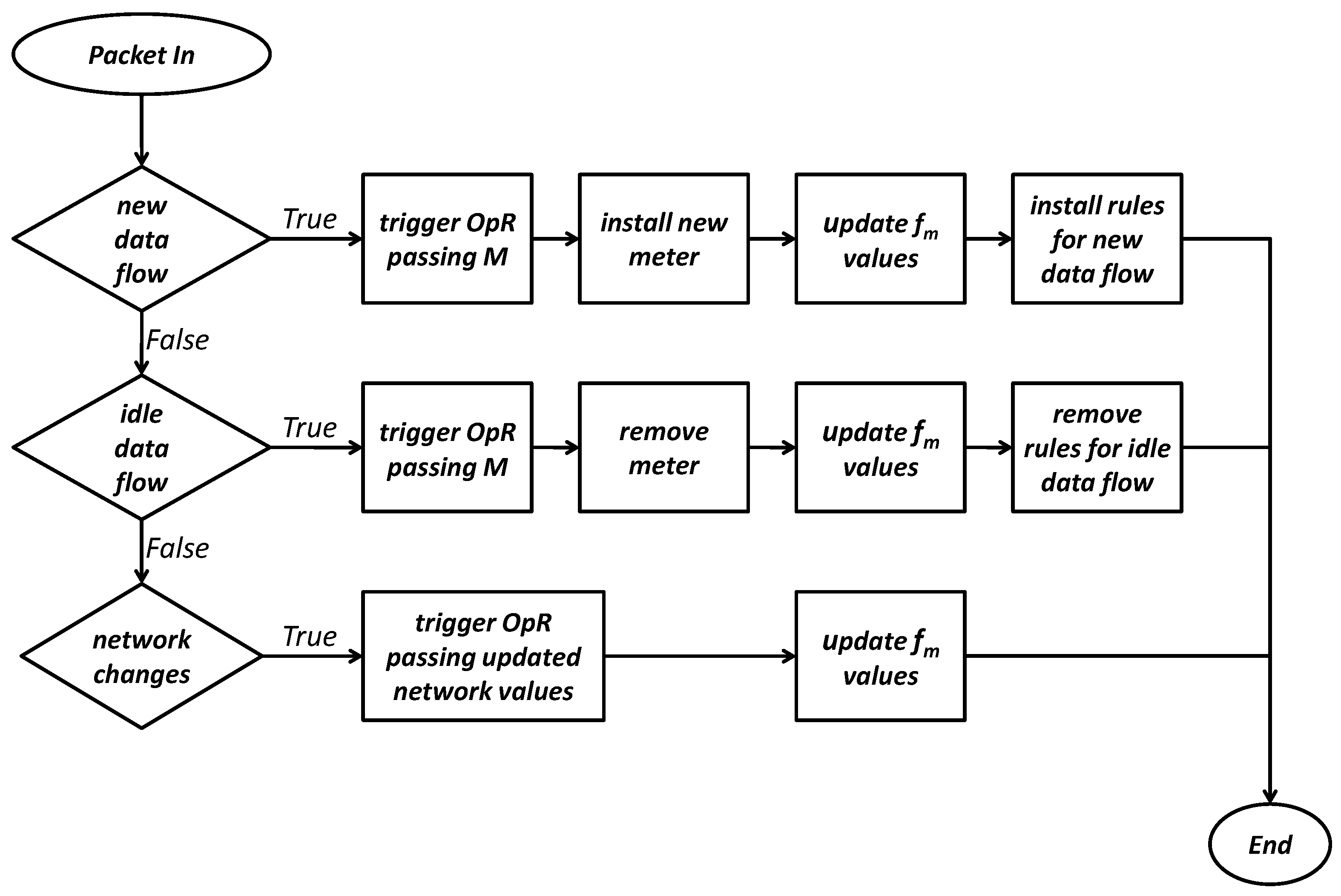
Figure 4.
Lifecycle of a data flow for a generic .
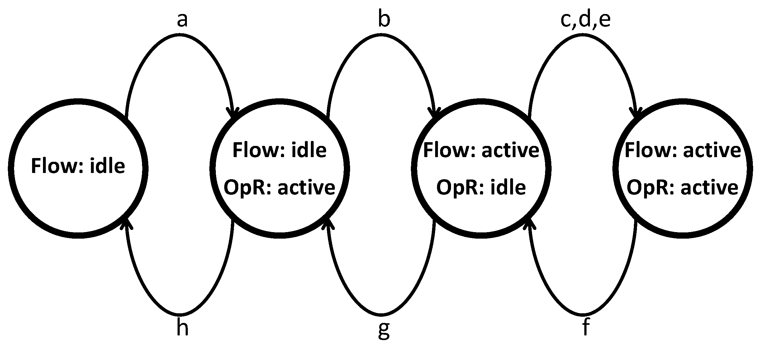
Figure 5.
IEEE 14-bus test network.

Figure 6.
Average uncertainty index for the voltage amplitude as a function of the bandwidth constraint both in the case of equally partitioned among the participating and in the case in which the developed optimization algorithm is applied.
Figure 6.
Average uncertainty index for the voltage amplitude as a function of the bandwidth constraint both in the case of equally partitioned among the participating and in the case in which the developed optimization algorithm is applied.
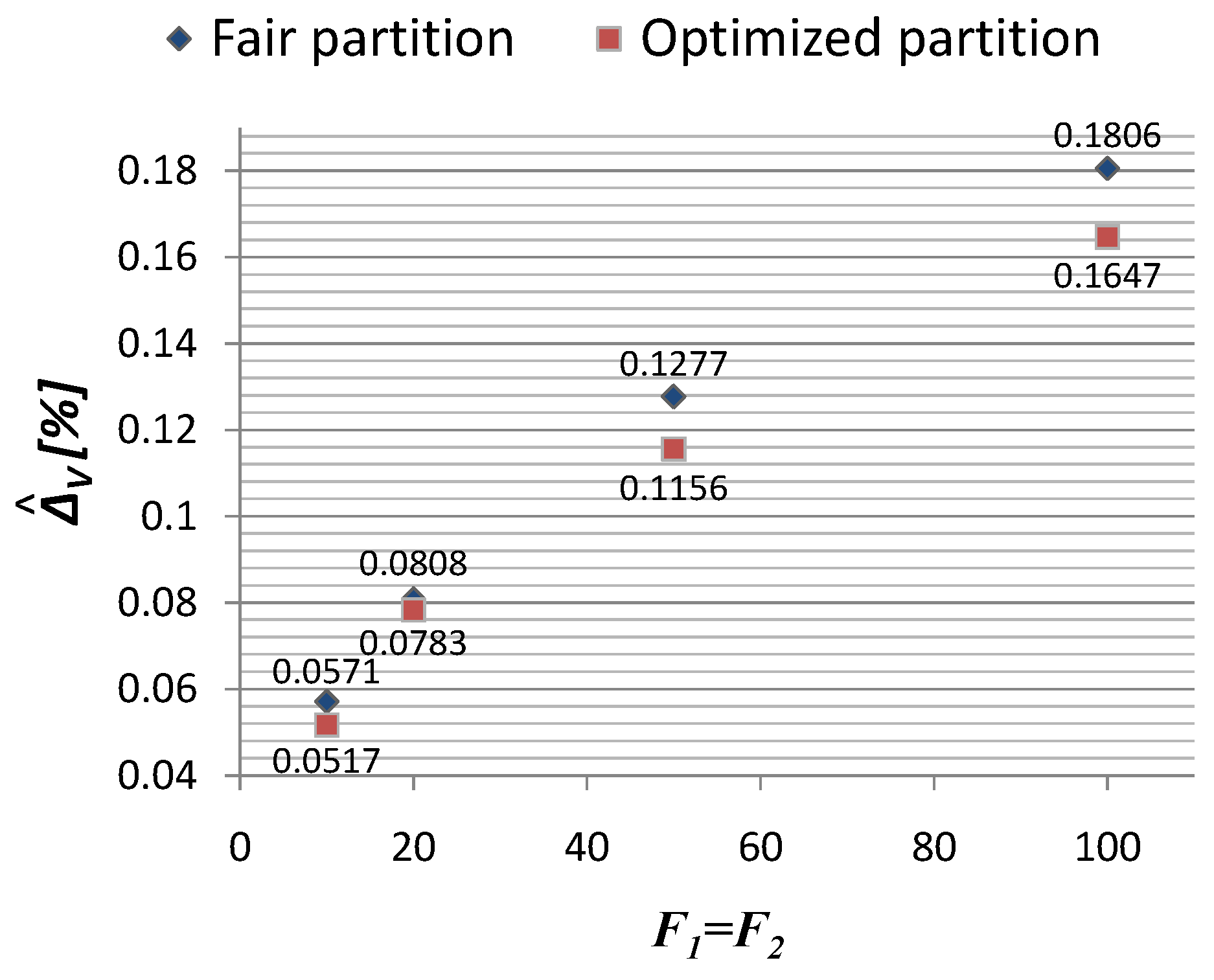
Figure 7.
Wireshark plot’s screenshot of the packet rate at the SE for the scenario with a change of at the two BFDs. PMU at node 2 has IP “”. PMU at node 6 has IP “”. PMU at node 7 has IP “”. PMU at node 9 has IP “”.
Figure 7.
Wireshark plot’s screenshot of the packet rate at the SE for the scenario with a change of at the two BFDs. PMU at node 2 has IP “”. PMU at node 6 has IP “”. PMU at node 7 has IP “”. PMU at node 9 has IP “”.

Figure 8.
Wireshark plot’s screenshot of the packet rate at the SE for the scenario in which the PMU at node 13 is removed. PMU at node 2 has IP “”. PMU at node 6 has IP “”. PMU at node 7 has IP “”. PMU at node 9 has IP “”. PMU at node 13 has IP “”.
Figure 8.
Wireshark plot’s screenshot of the packet rate at the SE for the scenario in which the PMU at node 13 is removed. PMU at node 2 has IP “”. PMU at node 6 has IP “”. PMU at node 7 has IP “”. PMU at node 9 has IP “”. PMU at node 13 has IP “”.


Table 1.
List of symbols for the considered system.
| MD with node index m | |
| M | Set of all MDs in the system |
| Cardinality of the set M | |
| Set of indexes of m | |
| BFD with index k | |
| K | Set of all BFDs in the system |
| Set of MDs attached to | |
| Bandwidth constraint on | |
| Bandwidth generated by | |
| Maximum reporting frequency of | |
| Granted reporting frequency to | |
| Size in bytes of a MD’s packet | |
| Packet rate constraint on |
Table 2.
List of events for the state diagram in Figure 4.
Table 2.
List of events for the state diagram in Figure 4.
| Events |
|---|
| a: No match for in the flow table and packet sent to the controller |
| b: Meter table installation on and flow rule installation on all involved FDs for ’s flow |
| c: A bandwidth change has been communicated by the hypervisor |
| d: A new MD different from the considered one has been installed/removed |
| e: The SE requested a new OpR run |
| f: The meter table of is updated |
| g: The idle_timeout for the flow of expired |
| h: The meter table and the flow rules for are removed |
Table 3.
PMU reporting frequency configurations in the case of both fair and optimized partitions.
| Constraints | Fair Partition | Optimized Partition |
|---|---|---|
| , | ||
| , | ||
| , | ||
| , |
Table 4.
Average uncertainty for the voltage amplitude when at the BFDs change and PMU accuracies are equal.
Table 4.
Average uncertainty for the voltage amplitude when at the BFDs change and PMU accuracies are equal.
| Constraints | Optimized Partition | [%] |
|---|---|---|
| , | ||
| , |
Table 5.
Average uncertainty for the voltage amplitude when at the BFDs change and PMU accuracies are different.
Table 5.
Average uncertainty for the voltage amplitude when at the BFDs change and PMU accuracies are different.
| Constraints | Optimized Partition | [%] |
|---|---|---|
| , | ||
| , | ||
| , |
Table 6.
Average uncertainty in case of PMU removal.
| Constraints | PMUs | Optimized Partition | [%] |
|---|---|---|---|
| , | 2,6,7,9,13 | ||
| 2,6,7,9 |
© 2017 by the authors. Licensee MDPI, Basel, Switzerland. This article is an open access article distributed under the terms and conditions of the Creative Commons Attribution (CC BY) license (http://creativecommons.org/licenses/by/4.0/).
Share and Cite
MDPI and ACS Style
Meloni, A.; Pegoraro, P.A.; Atzori, L.; Sulis, S. Bandwidth and Accuracy-Aware State Estimation for Smart Grids Using Software Defined Networks. Energies 2017, 10, 858. https://doi.org/10.3390/en10070858
AMA Style
Meloni A, Pegoraro PA, Atzori L, Sulis S. Bandwidth and Accuracy-Aware State Estimation for Smart Grids Using Software Defined Networks. Energies. 2017; 10(7):858. https://doi.org/10.3390/en10070858
Chicago/Turabian StyleMeloni, Alessio, Paolo Attilio Pegoraro, Luigi Atzori, and Sara Sulis. 2017. "Bandwidth and Accuracy-Aware State Estimation for Smart Grids Using Software Defined Networks" Energies 10, no. 7: 858. https://doi.org/10.3390/en10070858
Note that from the first issue of 2016, this journal uses article numbers instead of page numbers. See further details here.