SVR-Based Model to Forecast PV Power Generation under Different Weather Conditions

Abstract

Inaccurate forecasting of photovoltaic (PV) power generation is a great concern in the planning and operation of stable and reliable electric grid systems as well as in promoting large-scale PV deployment. The paper proposes a generalized PV power forecasting model based on support vector regression, historical PV power output, and corresponding meteorological data. Weather conditions are broadly classified into two categories, namely, normal condition (clear sky) and abnormal condition (rainy or cloudy day). A generalized day-ahead forecasting model is developed to forecast PV power generation at any weather condition in a particular region. The proposed model is applied and experimentally validated by three different types of PV stations in the same location at different weather conditions. Furthermore, a conventional artificial neural network (ANN)-based forecasting model is utilized, using the same experimental data-sets of the proposed model. The analytical results showed that the proposed model achieved better forecasting accuracy with less computational complexity when compared with other models, including the conventional ANN model. The proposed model is also effective and practical in forecasting existing grid-connected PV power generation.

1. Introduction

Energy, especially electrical energy, plays a key role in a country’s development; it also improves the living standard of people. Therefore, the demand for electrical energy has been increasing day by day due to industrialization and modernization. However, the conventional generation of electrical energy has caused global warming and significant climate changes. Subsequently, the modern world has undertaken different renewable energy initiatives to mitigate global warming and meet the growing electricity demand. Nowadays, many countries have produced a significant portion of their energy demands from renewable energy resources, particularly solar generation power plants [1]. Among the potential renewable energies, photovoltaics (PV) have undergone enormous growth over the last few years. The total installed capacity of PV systems has reached around 227 GW worldwide, an increase of more than 28% in 2015 (International Energy Agency (IEA) report, 2016); such growth is expected to continue at similar or higher rates in the future. Decreasing prices (i.e., the lowest at below $1.5/W_P for fixed tilt systems) and improved PV technology can also boost PV system installations [2,3].

However, the generation of PV power fully depends on random and ungovernable solar irradiance and other metrological factors, such as atmospheric temperature, module temperature, wind speed, wind direction, and humidity. The power output of a PV system dynamically changes with time due to the variability of environmental factors. Unpredictable PV power output adversely affects system stability and reliability, the scheduling of system operations, and related economic benefits [4,5]. Meanwhile, accurate forecasting of PV power generation can reduce the impact of PV power uncertainty on the grid, improve system reliability, maintain power quality, and increase the penetration level of PV systems [6]. Therefore, accurate forecasting of PV power generation has become an important task for researchers at present.

In a significant number of previous research, solar irradiance on different time scales was forecasted using various approaches, including numerical weather prediction methods, image-based methods, and statistical methods [7,8,9,10]. The forecasted solar irradiance and other associated data are used as inputs for PV power generation by commercial PV simulation software, such as TRNSYSM, PVFORM, and HOMER. In [11], first the fuzzy theorem was used to forecast the solar irradiance levels and then the recurrent neural network (RNN) method was used to forecast the 24 hour ahead output power of the PV system. However, most previous research on this problem employed direct methods to forecast PV power generation based on historical time-series data, such as historical PV power output and corresponding meteorological data. The research by Kudo et al. [12] demonstrated that the direct method of forecasting next-day PV power generation is better when compared with indirect methods.

In direct PV power forecasting, persistence modeling [13] is generally conducted to justify and select other models, and to decide on benchmarks. Persistence modeling is mainly used for one-hour ahead forecasting; hence, as the time range of forecasting increases, the accuracy of persistence modeling decreases [14]. Both autoregressive and moving-average modeling and their generalizations (i.e., autoregressive-moving-average models) [15] are widely used in statistical and time-series data analyses. These are based on classical time-series analysis such as following the Box–Jenkins method [16]. Yang et al. [17] proposed an autoregressive method, with an exogenous input (ARX)-based spatio-temporal (ST) model, in order to improve the accuracy of the developed PV output power forecasting technique. However, these time-series models have limitations because they require stationary data-sets [18]. A stationary time series is one whose statistical properties, such as mean, variance, and autocorrelation, are all constant over time. However, the PV power output and related meteorological data are non-stationary. By contrast, autoregressive-integrated-moving-average (ARIMA) models integrate non-stationarity elements from time-series data [19], but these models are computationally intensive because of the inclusion of a summation/integration function. The most general time series analysis model is called NARX (Nonlinear Autoregressive with Exogenous Input). In [20], NARX was chosen as a dynamic artificial neural network (ANN) to forecast the PV power generation, and the result showed that the NARX is more efficient because of its capability to learn and generalize formulas, compared with other ANN models. However, the NARX models have limitations in learning long time dependences because of the “vanishing gradient”. Furthermore, similar to any dynamical system, the models were affected by instability and lack a procedure for optimizing embedded memory. Moreover, time series models need lots of data when the model is structured, and the parameters are difficult to update when new data are uploaded.

ANN modeling is excellent for complicated and non-linear data analysis, and it does not require any prior assumption. Neural networks are widely used in PV power generation forecasting, and forecasted results are better when compared with those from regression analysis methods [21]. NARX and feed-forward neural networks with tapped delay lines have been used to forecast PV energy production, and they result in errors (MAPE) of less than 5% [22]. However, the performance of this forecasting model depends on meteorological factors and the correlation between explanatory variables and dependent variables. If the correlation factor between variables is less significant, then the forecasting result will be inaccurate. Multilayer perceptron (MLP) [23] is an example of the feed-forward NN model that has been widely deployed in PV power generation forecasting. In this model, the input of each neuron is transformed into output through the sigmoid function. The performance of this model is better than the Box–Jenkins method due to its non-linear approximation. The radial basis function neural network (RBFNN) [24] is a type of ANN model that makes use of linear combinations of radial basis functions. For the radial basis function, Gaussian functions are often used to transform inputs into outputs. If tuned accurately, the RBFNN has better performance than MLP. However, the tuning procedures of the RBFNN sometimes cause problems, such that good results are not obtained due to poor parameter adjustments. Among the ANN-based forecasting methods, back propagation NN (BPNN) has been widely used because of its excellent nonlinear mapping function, which is especially suitable for solving complex regression problems [25]. BPNN has the advantages of a complex nonlinear systems simulation ability, a strong learning ability, good approximation performance, and a large fault data tolerance. However, inherent defects are found, such as a slow convergence rate as well as a susceptibility to easily fall into local minimum values; thus BPNN is unable to obtain the global optimal solution [26].

Accuracy is a main consideration when developing models for PV power generation forecasting. For short-term forecasting, errors should be less than 20% [6]. However, for changing conditions (e.g., morning and evening, or rainy or cloudy weather), forecasting accuracy decreases to a point where the relative mean square errors (RMSE) are sometimes higher than 50%. To build better forecasting models, some studies classified forecasted days into different categories on the basis of weather conditions. Kang et al. [27] developed an algorithm by utilizing k-means clustering; Chen et al. [28] presented a RBFNN model; Shi et al. [6] proposed a model based on weather classification and support vector machines (SVM); Yang et al. [29] presented a weather-based hybrid method; and Liu et al. [26] proposed a back-propagation NN model to forecast PV power generation. All of these works classified days into different categories like sunny, cloudy, foggy, and rainy, and then built separate forecasting models for each classification. This approach implies that sub-models should be chosen on the basis of the weather condition of a forecasted day, apart from applying meteorological data to the model. However, although the accuracy is satisfactory for forecasting, sub-modeling is limited by complexity and computational costs.

In this paper, a generalized PV power forecasting model is proposed on the basis of support vector regression (SVR), historical data of PV power output, and meteorological data. In particular, SVR is supervised as a learning method and utilized for model development. In the study, PV power output characteristics and influential factors are analyzed to achieve forecasting accuracy. Subsequently, forecasted days are classified according to Malaysian weather conditions and historical PV power output data. The two types of weather in Malaysia are normal days (clear sky) and abnormal days (cloudy or rainy sky). Consequently, a generalized SVR-based model is introduced to forecast PV power generation accurately for any Malaysian weather condition. The proposed model is applied to and validated by three PV power stations situated in an institutional building of the University of Malaya in Kuala Lumpur. A generalized hourly resolution and day-ahead forecasting model is established to compare the forecasting accuracies of different weather conditions. This proposed single model, which is applicable for different weather conditions, is very simple to use and can reduce the complexities and computational costs.

The paper is organized as follows: Section 2 presents a brief description of the methods applied to forecast the PV power generation including real PV plant data collection and analysis; Section 3 indicates the performance metrics to evaluate the forecasting models; and Section 4 discusses the results of the proposed model including comparison and validations. Finally, Section 5 summarizes and concludes the study.

2. Methodology

2.1. Data Collection and Analysis

Three PV power generation systems were selected to collect PV power output and related meteorological data. These systems are located in Kuala Lumpur (latitude = 03°09′ N; longitude = 101°41′ E). The PV systems were installed on the rooftop of an institutional building of the University of Malaya.

Table 1. Details of photovoltaic (PV) power plants utilized in the study.

Data Sources	Nature of Plant	Installed Capacity	Measurement Items
Plant-1	Monocrystalline	1875 Wp (75 W × 25 pcs)	(i) PV power generation; (ii) Solar irradiance (W/m2); (iii) Atmospheric temperature (°C); (iv) PV module temperature (°C); (v) Wind speed (m/s)
Plant-2	Polycrystalline	2000 Wp (125 W × 16 pcs)
Plant-3	Thin-Film	2700 Wp (135 W × 20 pcs)

presents the details of these PV systems. The three PV plants are of monocrystalline, polycrystalline, and thin-film types with installed capacities of “1875”, “2000”, and “2700” Wp, respectively. PV power outputs were collected individually from each plant; however, meteorological data (i.e., solar irradiance, atmospheric temperature, module temperature, and wind pressure) were collected as a single dataset for all plants because of their similar geographical locations.

Table 2. Set of collected input/output variables of the PV system.

Input/Output Parameters		Unit	Resolution	Variables
Input Parameters	Solar Irradiance	W/m2	5 min	Irradiance
	Ambient Temperature	°C	5 min	Temp_amb
	Module Temperature	°C	5 min	Temp_module
	Wind Speed	m/s	5 min	Wind_speed
Output Parameter	PV Output Power	Watt	5 min	Power_pv

shows the collected data for each unit parameter identified for the study. The PV power output and related meteorological data were collected by an automatic data acquisition system in 5 min durations from 1 January 2016 to 31 December 2016.

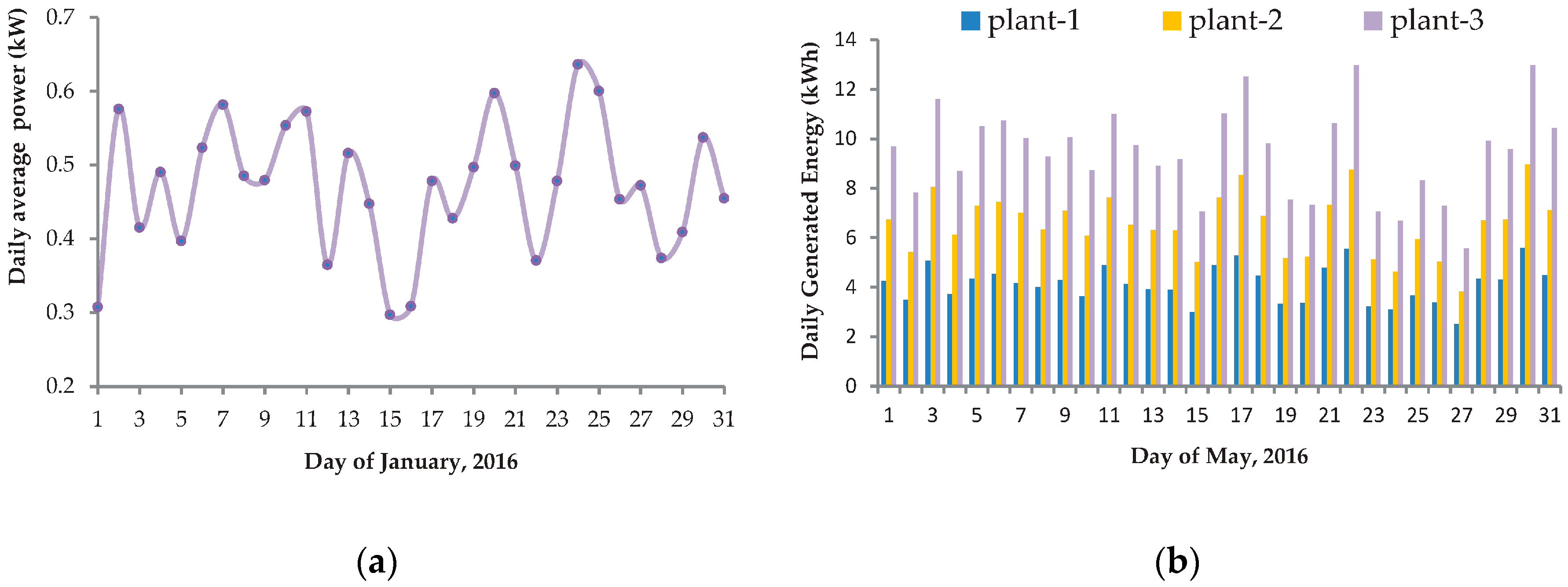
Figure 1a illustrates the mean daily PV power output generated by plant-1 for January 2016, and Figure 1b shows the daily energy generated by each PV plant for May 2016. Average power generation differed across days due to variations in the weather conditions.

For plant-1 (Figure 1a), the three days of 1, 15, and 16 January generated comparatively low power due to cloudy or rainy weather conditions (abnormal day). Meanwhile, due to clear skies (normal day), average power generation was comparatively higher for the days of 2, 7, 10, 11, 20, 24, and 25 January. In Figure 1b, the daily average PV energy production shows a rather stable fluctuation in relation to the different weather conditions in Malaysia, which suggests the potential of the country to generate PV energy.

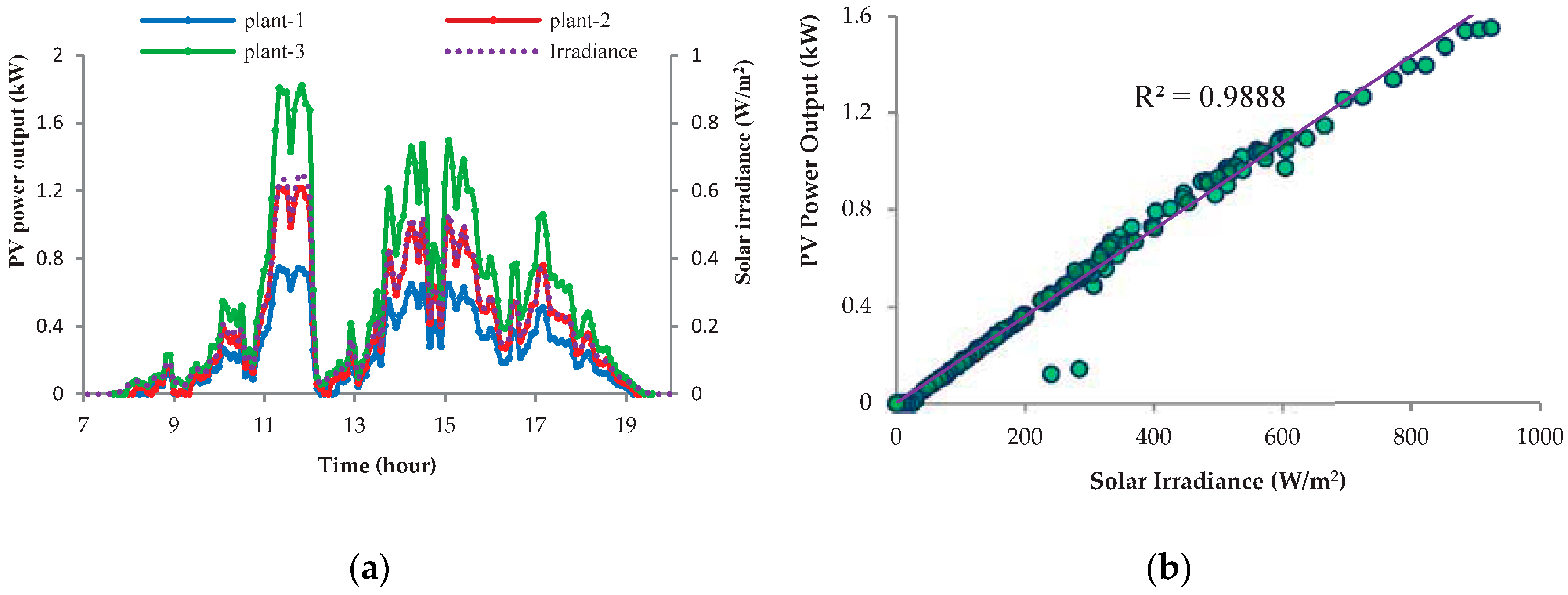
Photovoltaic power generation is closely related to meteorological parameters, such as solar irradiance, ambient/atmospheric temperature, module temperature, and wind speed, among others. Figure 2a shows the patterns of solar irradiance and PV power output of different PV plants on a particular day. During clear-sky days (normal day), PV power output very strongly matched the solar irradiance curve. Similarly, for cloudy or rainy days (abnormal day), a pattern harmony is observed between PV power output and solar irradiance as shown in Figure 2a. A similar pattern for PV power output and solar irradiance was observed for the different weather conditions because the generation of PV power fully depends on solar irradiance. If the irradiance increases, then PV power will be increased, and vice versa for any weather conditions. In Malaysian weather conditions, a linear relationship occurs between them. Therefore, a high correlation coefficient between PV power and solar irradiance has been observed. Figure 2b shows a strong positive correlation between solar irradiance and PV power output. Therefore, solar irradiance is an important input vector when developing an appropriate PV power forecasting model, as evidenced by the high correlation coefficient of R² = 0.9888.

The analytical results also indicate that the other meteorological variables, such as ambient temperature, module temperature, and wind pressure, were also correlated with PV power generation. A comparatively weak correlation was established between PV power output and atmospheric temperature, while an extremely weak correlation was observed between PV power output and wind speed. However, wind speed has been considered an input of the proposed model to build an appropriate model. By contrast, a strong correlation between PV power output and module temperature was observed. Nevertheless, it has been ignored in the selection as an input vector of the proposed model because the module temperature is highly dependent on other variables, such as atmospheric temperature, wind speed, wind direction, humidity, and the amount of PV power generation.

2.2. Data Preparation

Some meteorological variables showed extremely weak correlations with the PV power generation. In this study, the influence on PV power generation by all of the aforementioned independent meteorological variables was considered.

Sample data on actual PV power generated and related meteorological variables were collected at 5 min intervals. The obtained PV power output data and meteorological data were averaged as hourly datasets. However, during data collection, PV power output samples may be lost due to recording errors or other special events. If abnormal data are collected, the training of SVR becomes unstable. Thus, before averaging, missing data should be replaced by same-hours data from the latest similar day.

2.3. Pre-Processing of Data

The nonlinear SVR model can map nonlinear inputs into higher-dimensional space to make them linear. However, a wider data range results in imprecisions both in terms of fitting and regression. If data are pre-processed into smaller ranges before they are inputted into the model, then regression precision can be increased. A well-known solution to the aforementioned limitation is a normalization process, wherein data are restricted to the range of 0 and 1. Normalization minimizes regression error, improves precision, and maintains correlation in the data-set. The formula for normalization is [30]:

$$D_{\mathrm{Normal}}=\frac{D_{\mathrm{actual}}-D_{\min }}{D_{\max }-D_{\min }}$$

(1)

where $D_{\mathrm{Normal}}$ is the normalized input data; $D_{\mathrm{actual}}$ is the original input data (PV power output and meteorological data); and $D_{\min }$ and $D_{\max }$ are the minimum and maximum values of the utilized input data, respectively.

2.4. Support Vector Regression

SVM [31] is a supervised machine-learning method that follows the structural risk minimization principle. SVMs have greater generalization ability compared with other approaches, and they are widely used in resolving classification and regression problems. SVMs are excellent for time-series analysis due to its global minima. When applied to time-series prediction, SVM modeling is referred to as support vector regression (SVR). Forecasting PV power generation is a typical time-series analysis problem; in this case, SVR is an appropriate method.

The SVR algorithm is a nonlinear regression algorithm. Inputs from time-series data samples are mapped into high-dimensional feature space for nonlinear mapping. Subsequently, linear regression is conducted (Figure 3).

A set of training data $\left\{\left(x_1,y_1\right), \left(x_2,y_2\right),\dots \dots ,\left(x_l, y_l\right)\right\}$ is considered, where $x_i\in R^n$ is the input vector (meteorological data), and $y_i\in R^1$ is the corresponding output value (PV power output). The estimation function $f\left(x\right)$ is shown in Function (2):

$$y=f\left(x\right)=w\times \psi \left(x\right)+b$$

(2)

where $w\in R^n$ is a weight vector, and $b\in R$ is the bias term, which can be estimated by minimizing the regularized risk function.

Using the $\epsilon$-insensitive loss function in SVR, the regression problem can be changed into the following optimization problem:

$$\begin{gathered} \min : \frac{1}{2}\mathrm{ǀ}\mathrm{ǀ}w\mathrm{ǀ}{\mathrm{ǀ}}^2+C{\displaystyle \sum }_{i=1}^l\left({\xi }_i+{\xi }_i^{*}\right) \\ \text{Subject} \text{to}: y_i-f\left(x\right)\le \epsilon +{\xi }_i^{*}; f\left(x\right)-y_i\le \epsilon +{\xi }_i; \text{and} {\xi }_i^{*},{\xi }_i\ge 0 \end{gathered}$$

(3)

where $\epsilon$ is the radius of the tube (margin of tolerance), which refers to the data inside the tube that should be ignored during regression. The feature vector, which lies on the boundary of the tube, is known as the support vector.

In line with the Lagrange multiplier method, the Lagrange function is acquired as follows:

$$\begin{gathered} L\left(w,b,\xi ,{\xi }^{*},\alpha ,{\alpha }^{*},\gamma ,{\gamma }^{*}\right)=\frac{1}{2}\mathrm{ǀ}\mathrm{ǀ}w\mathrm{ǀ}{\mathrm{ǀ}}^2+C{\displaystyle \sum }_{i=1}^l\left(\xi +{\xi }^{*}\right)-{\displaystyle \sum }_{i=1}^l{\alpha }_i\mathrm{ǀ}{\xi }_i+\epsilon -y_i+f\left(x_i\right)\mathrm{ǀ} \\ -{\displaystyle \sum }_{i=1}^l{\alpha }_i^{*}\mathrm{ǀ}{\xi }_i^{*}+\epsilon +y_i-f\left(x_i\right)\mathrm{ǀ}-{\displaystyle \sum }_{i=1}^l\left({\xi }_i{\gamma }_i+{\xi }_i^{*}{\gamma }_i^{*}\right) \end{gathered}$$

(4)

where $\xi \mathrm{and} {\xi }^{*}$ are the slack variables representing the distance from actual values to the corresponding boundary values of the ε-tube. Hence, $\alpha ,{\alpha }^{*},\gamma ,{\gamma }^{*}\ge 0.$

Next, the saddle point of L is calculated. The following equations can thus be obtained:

$$\begin{gathered} \frac{\partial }{\partial w}L=0 \Rightarrow w={\displaystyle \sum }_{i=1}^l({\alpha }_i-{\alpha }_i^{*})\psi (x_i) \\ \frac{\partial }{\partial b}L=0 \Rightarrow {\displaystyle \sum }_{i=1}^l({\alpha }_i-{\alpha }_i^{*})=0 \\ \frac{\partial }{\partial {\xi }_i}L=0 \Rightarrow C-{\alpha }_i-{\gamma }_i=0 \end{gathered}$$

(5)

By substituting the original Function (4) with Equation (5), the following model can be obtained:

$$\begin{gathered} max: \overline{w}{(\alpha ,{\alpha }^{*})}_{w,b,\xi ,{\xi }^{*}}=-\frac{1}{2}{\displaystyle \sum }_{i,j=1}^l\left({\alpha }_i-{\alpha }_i^{*}\right)\left({\alpha }_j-{\alpha }_j^{*}\right)<\psi (x_i),\psi (x_j)> \\ -{\displaystyle \sum }_{i=1}^l({\alpha }_i+{\alpha }_i^{*})\epsilon +{\displaystyle \sum }_{i=1}^l({\alpha }_i-{\alpha }_i^{*})y_i \\ Subject to: {\displaystyle \sum }_{i=1}^l({\alpha }_i-{\alpha }_i^{*})=0; 0\le {\alpha }_i,{\alpha }_i^{*}\le C \end{gathered}$$

(6)

where C determines the penalties of the estimation errors.

Subsequently, the kernel function $k\left(x_i,x_j\right)$ is introduced with a mercer condition to replace the original function $<\psi \left(x_i\right),\psi \left(x_j\right)>,$ and the following model can thus be obtained:

$$\begin{gathered} max:\overline{w}{(\alpha ,{\alpha }^{*})}_{w,b,\xi ,{\xi }^{*}}=-\frac{1}{2}{\displaystyle \sum }_{i,j=1}^l({\alpha }_i-{\alpha }_i^{*})\left({\alpha }_j-{\alpha }_j^{*}\right)k(x_i,x_j) \\ -{\displaystyle \sum }_{i=1}^l({\alpha }_i+{\alpha }_i^{*})\epsilon +{\displaystyle \sum }_{i=1}^l({\alpha }_i-{\alpha }_i^{*})y_i \\ Subject to: {\displaystyle \sum }_{i=1}^l({\alpha }_i-{\alpha }_i^{*})=0; 0\le {\alpha }_i,{\alpha }_i^{*}\le C \end{gathered}$$

(7)

The kernel function is one of the key factors of SVR. The performance of SVR is largely dependent on the selection of the kernel function and its parameters. Four traditional kernel functions are commonly used in SVR:

• Liner kernel function: $k\left(x_i,x_j\right)=x_i^T{x}_j;$
• Polynomial: $k\left(x_i,x_j\right)={(\gamma x_i^T{x}_j+r)}^d, \gamma >0;$
• Gaussian RBF (radial bias function): $k\left(x_i ,x_j\right)=exp\left(-\frac{\mathrm{ǀ}\mathrm{ǀ}{x}_i-x_j\mathrm{ǀ}{\mathrm{ǀ}}^2}{2{\sigma }^2}\right)=\mathit{exp}\left(-\gamma \mathrm{ǀ}\mathrm{ǀ}{x}_i-x_j\mathrm{ǀ}{\mathrm{ǀ}}^2\right), \gamma >0;$
• Sigmoid: $k\left(x_i,x_j\right)=\mathit{tanh}\left(\gamma x_i^T{x}_j+r\right).$

The radial bias function (RBF) is often used as the kernel in SVR because it requires only one parameter and it has a wide scope of application. RBFs also have the ability to universally approximate any distribution in feature space. Therefore, the RBF was used as kernel in this study. For the RBF, ${\sigma }^2$ was set as the bandwidth of the kernel function.

To optimally solve the problems, the best ${\alpha }_i \mathrm{and} {\alpha }_i^{*}$ should be obtained. The best-fit regression function can be expressed as follows:

$$f(x)={\displaystyle \sum }_{i=1}^l({\alpha }_i-{\alpha }_i^{*})\times k\left(x_i,x_j\right)+b$$

(8)

where ${\alpha }_i$ and ${\alpha }_i^{*}$ are the Lagrange multipliers; and $k\left(x_i, x_j\right)$ is the kernel function. The nonlinear separable cases can be easily transformed into linear cases by mapping the original variable into a new high-dimension feature space using $k\left(x_i, x_j\right)$.

2.5. Proposed SVR-Based Model to Forecast PV Power Generation

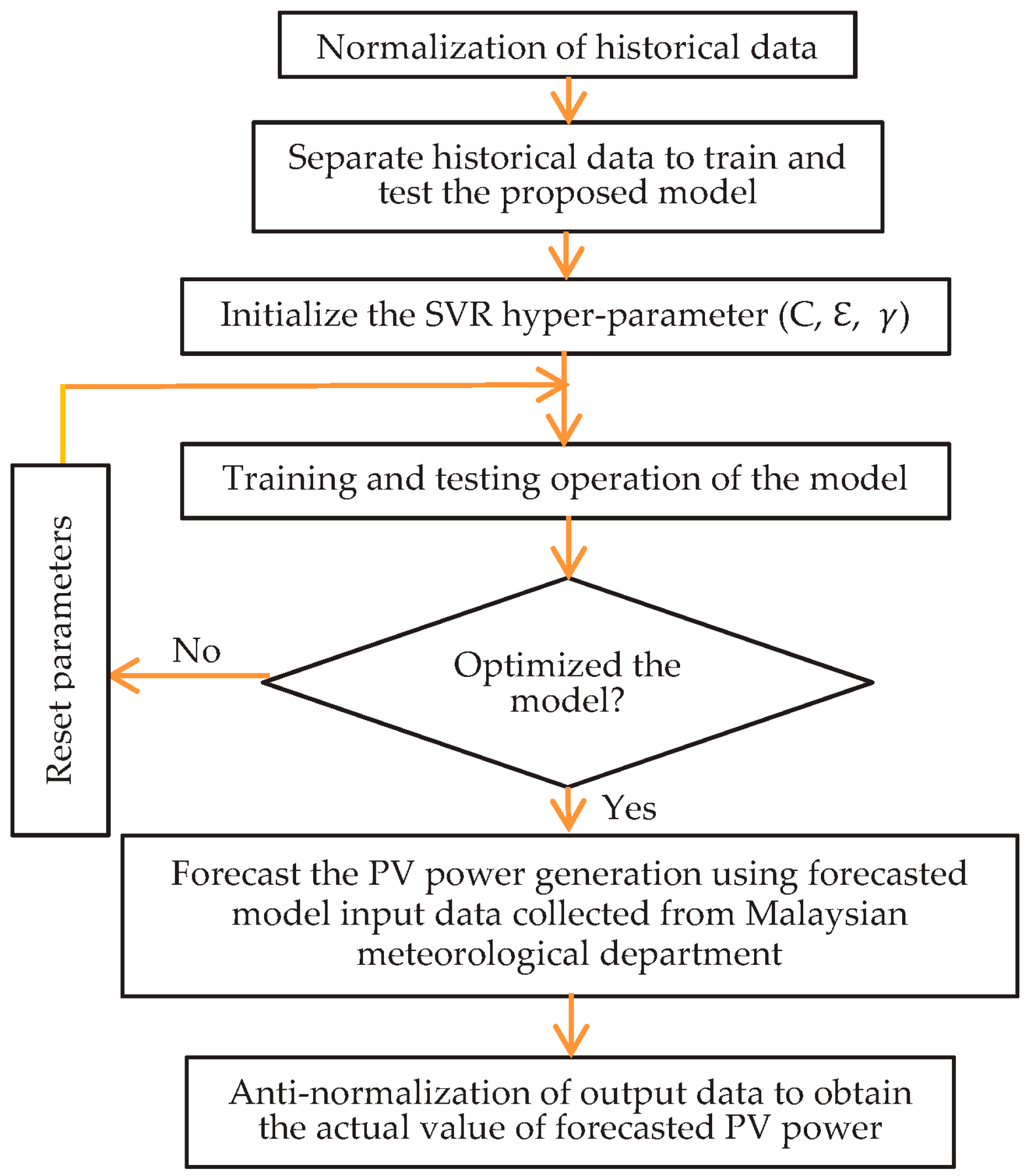
To establish the generalized SVR-based model for PV power generation forecasting, the LIBSVM package [32] proposed by Chang and Lin (2001) was adopted in present study. For the proposed generalized day-ahead hourly resolution model using the SVR approach, the average hourly data samples were considered for training and testing purposes. The diagram flow of the proposed model is shown in Figure 4.

Historical data of meteorological variables (i.e., solar irradiance, atmospheric temperature, and wind speed) were considered as the input data-set of the model. Meanwhile, historical data of PV power output were considered as the output data-set for training the proposed model. All of the original historical PV power data and meteorological data were normalized within the range of [0, 1] to minimize regression error. Subsequently, the datasets for training (i.e., more than 70% of the total data) and testing were separated. To develop the model, the initialization values of the three dominating parameters (C, $\epsilon$, and γ) in SVR should be also included. The training and the testing of the model were conducted first-time using the stipulated historical data-set. A non-optimization model implies that the dominating parameter values should be changed, and model training and testing should be conducted again; this procedure should be continued until the model is optimized. In the present study, the parameters were chosen on the basis of experience-based trial and error. An optimized model implies that PV power generation can be forecasted for a particular day. To forecast PV power generation using the proposed model, the hourly averages of normalized meteorological data for a given forecasted day (i.e., data collected from the Malaysian meteorological department or numerical predicted data) should be applied. Given that the input data of this model were normalized, the output data should be anti-normalized to extract the original values of PV power; this process consolidates the performance analysis of the proposed model.

A standard three-layer back-propagation ANN with the number of epochs set to 1000 was utilized as the alternative model for a comparative evaluation of the performance of the proposed model. To evaluate for better performance of the ANN model, the number of hidden neurons of the ANN model was changed to be between 5 and 20. To establish the benchmark of the PV power forecasting model, a persistence model was used to validate the proposed model.

3. Evaluation of Forecasting Accuracy

Several types of performance metrics were used to evaluate the accuracy of the forecasting model. In this study, normalized root-mean-square error (nRMSE) (i.e., the most commonly used metric), mean absolute error (MAE), and mean bias error (MBE) were adopted for the proposed model:

$${\mathrm{nRMSE}}_{\%}=\left(\sqrt{\frac{1}{N} {\displaystyle \sum }_{i=1}^N{\left(W_{\mathrm{Predicted}}-W_{\mathrm{actual}}\right)}^2}\right)\times 100/W_{\mathrm{actual}\left(\max \right)}$$

(9)

$$\mathrm{MAE}=\frac{1}{N}{\displaystyle \sum }_{i=1}^N\left|W_{\mathrm{Predicted}}-W_{\mathrm{actual}}\right|$$

(10)

$$\mathrm{MBE}=\frac{1}{N}{\displaystyle \sum }_{i=1}^N\left(W_{\mathrm{Predicted}}-W_{\mathrm{actual}}\right)$$

(11)

where $W_{\mathrm{predicted}}$ and $W_{\mathrm{actual}}$ are the forecasted value and actual measured value of the PV power output at each time point, respectively. In addition, $W_{\mathrm{actual}\left(\max \right)}$ is the maximum value of the actual measured PV power output, and N is the number of test data samples. The datasets for training and testing were normalized; accordingly, the forecasted PV power output data of the model have to be anti-normalized before calculating the nRMSE, MAE, and MBE.

4. Result and Discussion

In this research, a generalized forecasting model based on SVR was developed. The model was applied for hourly resolution day-ahead PV power generation forecasting. The actual PV power generation data of three different PV plants and their related meteorological data (i.e., solar irradiance, atmospheric temperature, and wind speed) were utilized in the study. In Malaysia, solar irradiance is available from 08:00 to 19:00 at almost all seasons of the year; accordingly, daily PV power outputs are received during these times only. Experimental data covering three months (January, May, and September 2016) were used to verify the proposed model. However, Malaysian weather conditions have not changed drastically over the year. Nevertheless, these three months have been selected in this analysis because all of the weather conditions throughout the year were considered. Sample data were selected randomly for training and test purposes due to different weather conditions. The forecasted PV power of the proposed model should be anti-normalized to extract the actual value of the PV power forecast. Consequently, the forecasted values of the proposed model were compared with those for the standard back-propagation NN model and the persistence model.

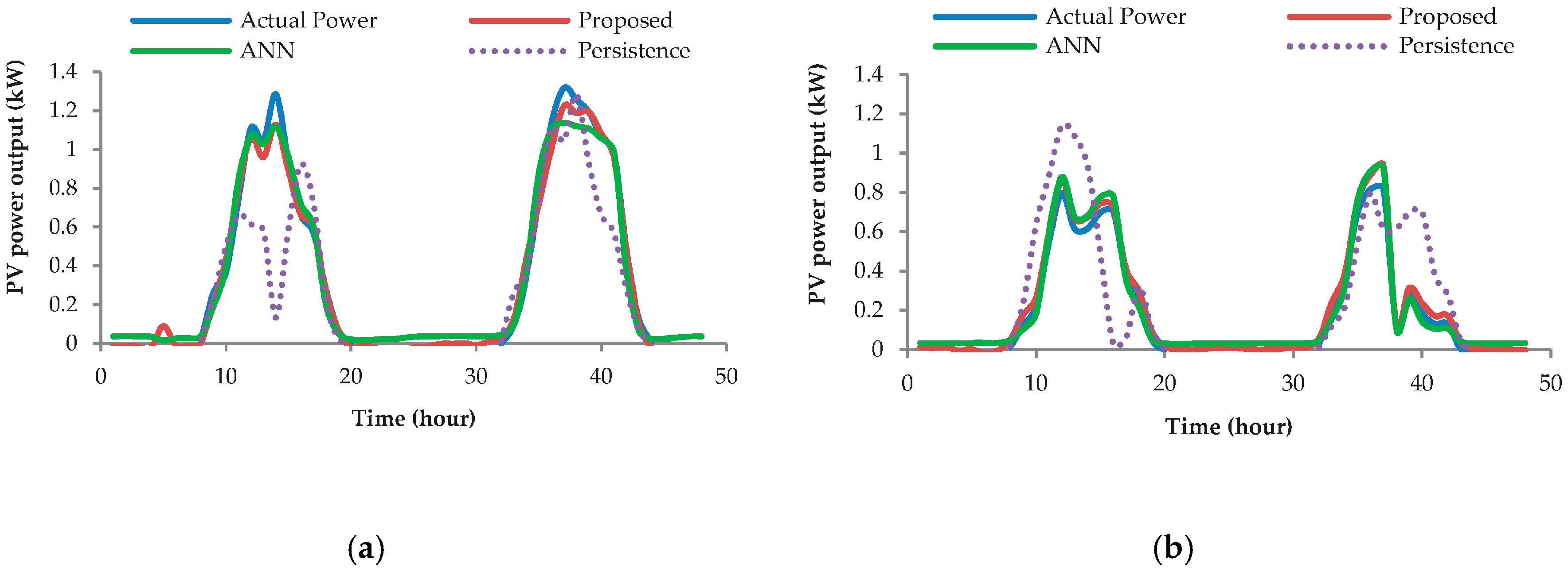
Figure 5a shows the measured PV power outputs (actual) and forecasted PV power outputs of the different models (i.e., proposed model, ANN, and persistence model) of PV plant-1 in normal weather conditions. In this case, 21 and 22 May were set as the forecast days. As shown in Figure 1b and based on the analysis of the PV power output patterns, these days (21 and 22 May) are clear-sky days (normal day). Hence, the hourly PV power output average and related metrological data of 14 days (7–20 May) were used to train the model. As shown in Figure 5a, the forecasted curve of the proposed model almost matched the actual measured curve of PV power generation.

Figure 5b represents the actual measured PV power outputs and forecasted PV power outputs of the proposed model, ANN model, and persistence model of plant-1 in abnormal weather conditions. In this figure, 26 and 27 May were set as forecast day. As shown in Figure 1b and based on the analysis of PV power output patterns, these days are cloudy or rainy days (abnormal day). Hence, the hourly PV power output average and related meteorological data of 14 days (12–25 May) were used to train the model. As shown in Figure 5b, the forecasted curve of the proposed model almost matched the actual measured curve of PV power generation. However, a significant deviation for the persistence model curve was observed, which might have been affected by abnormal weather conditions.

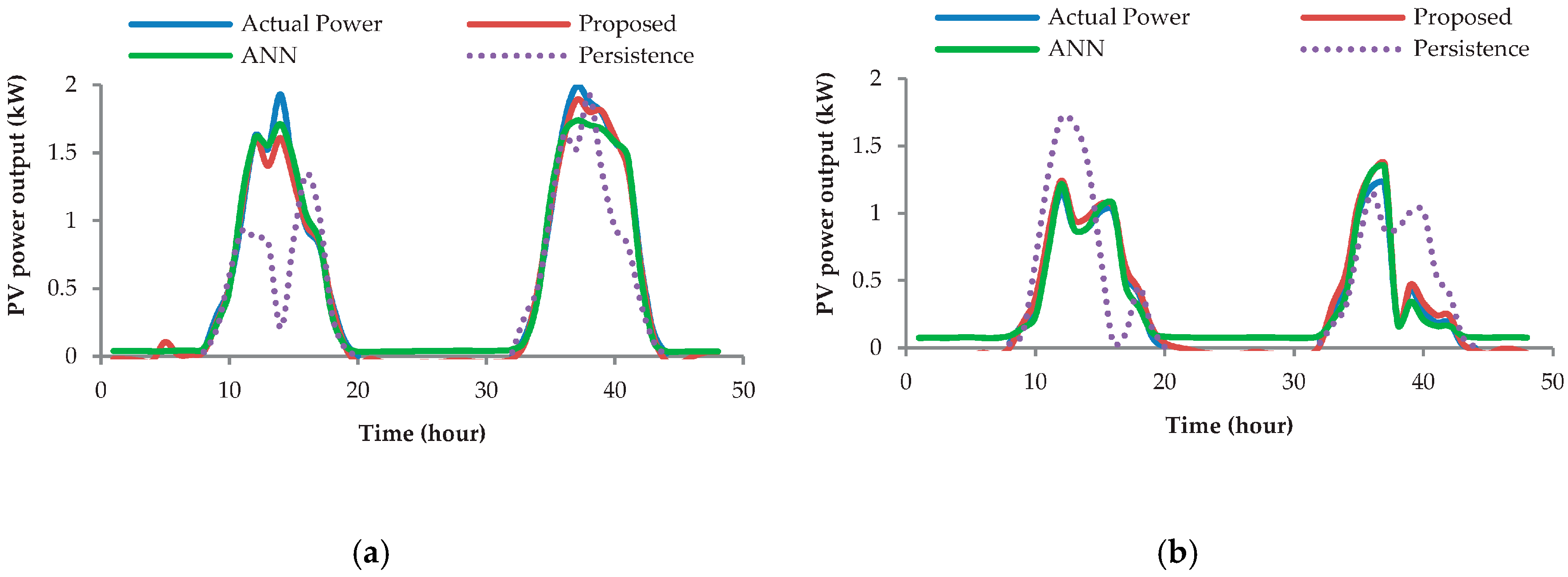
The same meteorological data-set and related PV power output data of PV plant-2 were used to train and test the models in different weather conditions. Similarly to plant-1, normal forecast days (21 and 22 May) and abnormal forecast days (26 and 27 May) were selected. Figure 6a,b shows the actual measured PV power output and forecasted PV power output of the different models (i.e., the proposed model, the ANN model, and the persistence model) for normal and abnormal weather conditions, respectively. As shown by Figure 6a,b, the forecasted result of the proposed model almost matched the actual measured PV power output of plant-2.

Similarly to the previous approach, the same meteorological data-set and related PV power output data of plant-3 were used to train and test the proposed model, the ANN model, and the persistence model in different weather conditions. Normal and abnormal forecast days were selected, similarly to plant-1 and plant-2, in consideration of same-month data. Figure 7a,b shows the actual measured PV power output and forecasted PV power output of the different models for normal and abnormal weather conditions, respectively. The figures show that the proposed PV power curve almost matched the actual measured PV power curve of plant-3.

The performances of the proposed model, the ANN model, and the persistence model were evaluated using the experimental data of May 2016. In this case, nRMSE, MAE, and MBE were adopted for the forecasting performance evaluation. Calculation results are shown in

Table 3. Summary of the forecasting performance for the data of May 2016.

Metrics	Models	Plant-1	Plant-2	Plant-3	Mean	Average
nRMSE (%)	Proposed	N = 2.77	N = 2.56	N = 2.58	N = 2.64	3.06
		A = 3.66	A = 3.53	A = 3.21	A = 3.47
	ANN	N = 3.53	N = 3.32	N = 3.45	N = 3.43	3.83
		A = 4.58	A = 4.47	A = 3.65	A = 4.23
	Persistence	N = 15.97	N = 15.64	N = 14.81	N = 15.47	16.22
		A = 17.25	A = 16.97	A = 16.68	A = 16.97
MAE (W)	Proposed	N = 17.12	N = 24.87	N = 46.99	N = 29.66	32.36
		A = 23.81	A = 34.68	A = 46.65	A = 35.05
	ANN	N = 25.51	N = 40.74	N = 66.62	N = 44.29	44.26
		A = 27.94	A = 46.48	A = 58.27	A = 44.23
	Persistence	N = 72.40	N = 120.43	N = 170.47	N = 121.10	115.36
		A = 64.04	A = 106.50	A = 158.30	A = 109.61
MBE (W)	Proposed	N = 6.91	N = 23.38	N = 6.56	N = 12.28	16.11
		A = 13.86	A = 16.59	A = 29.35	A = 19.93
	ANN	N = 14.89	N = 23.79	N = 34.77	N = 24.48	14.42
		A = 3.95	A = 4.68	A = 4.41	A = 4.35
	Persistence	N = 23.93	N = 44.13	N = 57.38	N = 41.81	60.39
		A = 45.56	A = 73.30	A = 118.05	A = 78.97

Hence, “N” means normal day and “A” means abnormal day. “nRMSE” means normalized root-mean-square error. “MAE” means mean absolute error. “MBE” means mean bias error.

.

Similar work has been done by using other practical datasets collected from the months of January and September of 2016 for further validation of the proposed model. In this case, the analyses have been completed by considering the normal and abnormal weather conditions separately. From the analysis of the PV power output pattern of January, it is clear that 24 and 25 January are normal days, and 15 and 16 January are abnormal days. On the other hand, it is also clear from the analysis of the PV power output pattern of September that 29 and 30 September are normal days and 21 and 22 September are abnormal days. From this study, it has been found that the actual measured output and forecasting output of the proposed model are almost matched in all PV plants for the data-sets of both months. The detail of the error calculation result is shown in

Table 4. Summary of the forecasting performance for the data of January 2016.

Metrics	Models	Plant-1	Plant-2	Plant-3	Mean	Average
nRMSE (%)	Proposed	N = 2.78	N = 2.27	N = 2.96	N = 2.67	3.12
		A = 3.96	A = 3.46	A = 3.30	A = 3.57
	ANN	N = 4.16	N = 3.24	N = 3.17	N = 3.52	3.86
		A = 4.27	A = 4.11	A = 4.20	A = 4.19
	Persistence	N = 12.99	N = 13.34	N = 13.61	N = 13.31	13.03
		A = 13.32	A = 12.49	A = 12.41	A = 12.74
MAE (W)	Proposed	N = 19.71	N = 23.41	N = 36.93	N = 26.68	33.63
		A = 24.57	A = 36.49	A = 60.66	A = 40.57
	ANN	N = 28.90	N = 39.42	N = 67.48	N = 45.27	50.69
		A = 32.36	A = 50.37	A = 85.57	A = 56.10
	Persistence	N = 68.48	N = 108.33	N = 170.47	N = 115.76	109.17
		A = 60.89	A = 96.21	A = 150.60	A = 102.57
MBE (W)	Proposed	N = 10.62	N = 5.65	N = 11.98	N = 9.42	8.08
		A = 10.43	A = 2.32	A = 7.45	A = 6.73
	ANN	N = 9.62	N = 6.58	N = 14.62	N = 10.27	12.52
		A = 20.79	A = 8.93	A = 14.58	A = 14.77
	Persistence	N = 28.99	N = 49.81	N = 76.00	N = 51.60	45.88
		A = 25.47	A = 37.49	A = 57.52	A = 40.16

for the month of January and

Table 5. Summary of the forecasting performance for the data of September 2016.

Metrics	Models	Plant-1	Plant-2	Plant-3	Mean	Average
nRMSE (%)	Proposed	N = 2.85	N = 2.67	N = 2.72	N = 2.75	3.06
		A = 3.71	A = 3.36	A = 3.04	A = 3.37
	ANN	N = 3.31	N = 3.03	N = 3.11	N = 3.15	3.90
		A = 5.02	A = 4.73	A = 4.16	A = 4.64
	Persistence	N = 10.80	N = 11.47	N = 11.42	N = 11.23	10.45
		A = 8.95	A = 10.16	A = 9.88	A = 9.66
MAE (W)	Proposed	N = 22.02	N = 34.64	N = 53.82	N = 36.83	37.72
		A = 23.24	A = 40.70	A = 51.89	A = 38.61
	ANN	N = 26.39	N = 41.45	N = 65.14	N = 44.33	51.54
		A = 35.68	A = 60.63	A = 79.95	A = 58.75
	Persistence	N = 44.27	N = 75.78	N = 113.62	N = 77.89	78.25
		A = 40.94	A = 77.90	A = 117.00	A = 78.61
MBE (W)	Proposed	N = 2.40	N = 11.92	N = 21.83	N = 12.05	9.82
		A = 8.43	A = 9.61	A = 4.71	A = 7.58
	ANN	N = 11.81	N = 23.67	N = 27.10	N = 20.86	13.81
		A = 3.85	A = 3.47	A = 12.93	A = 6.75
	Persistence	N = 25.31	N = 48.19	N = 75.27	N = 49.59	34.37
		A = 4.87	A = 20.42	A = 32.13	A = 19.14

for the month of September.

The performances of the proposed model, the ANN model, and the persistence model were calculated by averaging the performance values for the three-month period (

Table 6. Summary of overall forecasting performance.

Metrics	Methods	Average (January)	Average (May)	Average (September)	Average (Proposed Model)	Average (ANN Model)	Average of Persistence Model	Other ANN Models [33]
nRMSE (%)	Proposed	3.12	3.06	3.06	3.08	3.86	13.23	5.95
	ANN	3.86	3.83	3.90
	Persistence	13.03	16.22	10.45
MAE (W)	Proposed	33.63	32.36	37.72	34.57	48.83	100.93	-
	ANN	50.69	44.26	51.54
	Persistence	109.17	115.36	78.25
MBE (W)	Proposed	8.08	16.11	9.82	11.34	13.58	46.88	-
	ANN	12.52	14.42	13.81
	Persistence	45.88	60.39	34.37

). This table shows the average nRMSE, MAE, and MBE result for the different models. The overall average result for the different models and those for other ANN-based forecasting models [33] are also presented in Table 6.

Based on the figures, tables, and discussions presented in this paper, the proposed generalized SVR-based model performed very well for PV power generation forecasting in different weather conditions. The results also showed that the model could forecast the PV power generation accurately in various seasonalities of Malaysian weather conditions. The errors obtained for all of the plants using the proposed model are very similar for normal and abnormal weather conditions. In the proposed model, the errors computed in normal weather conditions are always slightly lower compared with those for the abnormal weather conditions. The reason for this situation is that the model can be fitted well in normal weather conditions because of less variation in sample data. Hence, the forecasted results are nearly the same in various months because of the absence of drastic changes in the weather conditions of Malaysia. The average forecasting results of the proposed model were 3.08% in nRMSE, 34.57 W in MAE, and 11.34 W in MBE, which were better compared with the ANN model and the persistence model. The proposed model also outperformed other ANN-based forecasting models [33].

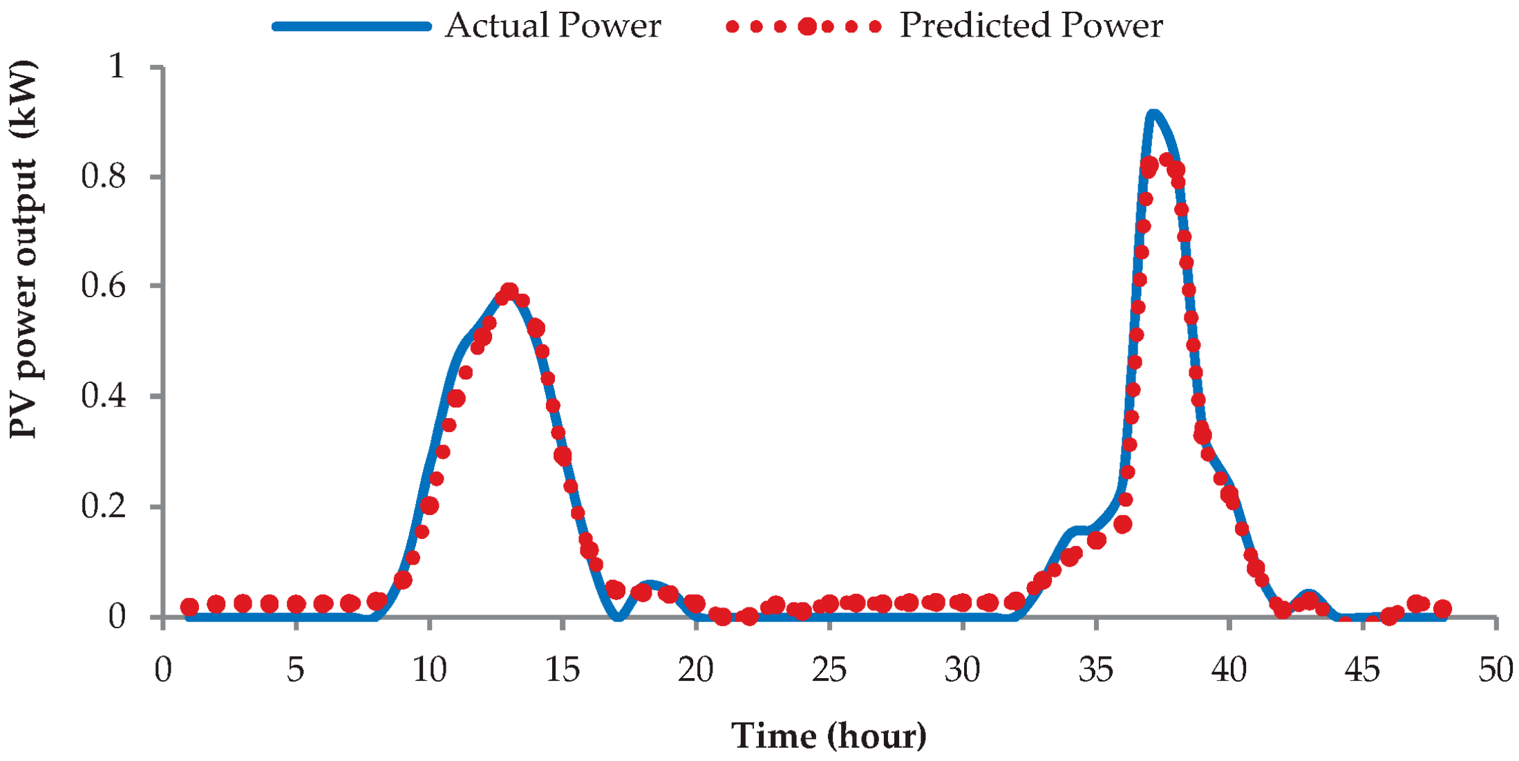
Figure 8 shows the actual measured PV power output and the forecasted PV power output of the proposed model. In this case, 14 and 15 January were set as forecast days. As shown in Figure 1a and based on the PV power output pattern of plant-1, these two days have cloudy or rainy weather conditions (abnormal day), which suggest comparatively low electrical energy. The shape of the second part of this figure is quite different from the other figures because some hours during these days have clear skies while the rest are cloudy or rainy. However, the highest peak of the first part of the figure is comparatively low due to the existence of some clouds that day. Nonetheless, the forecasting PV power of the proposed model almost matched the actual measured PV power in any situation. Therefore, the proposed model can forecast PV power generation accurately in any weather condition.

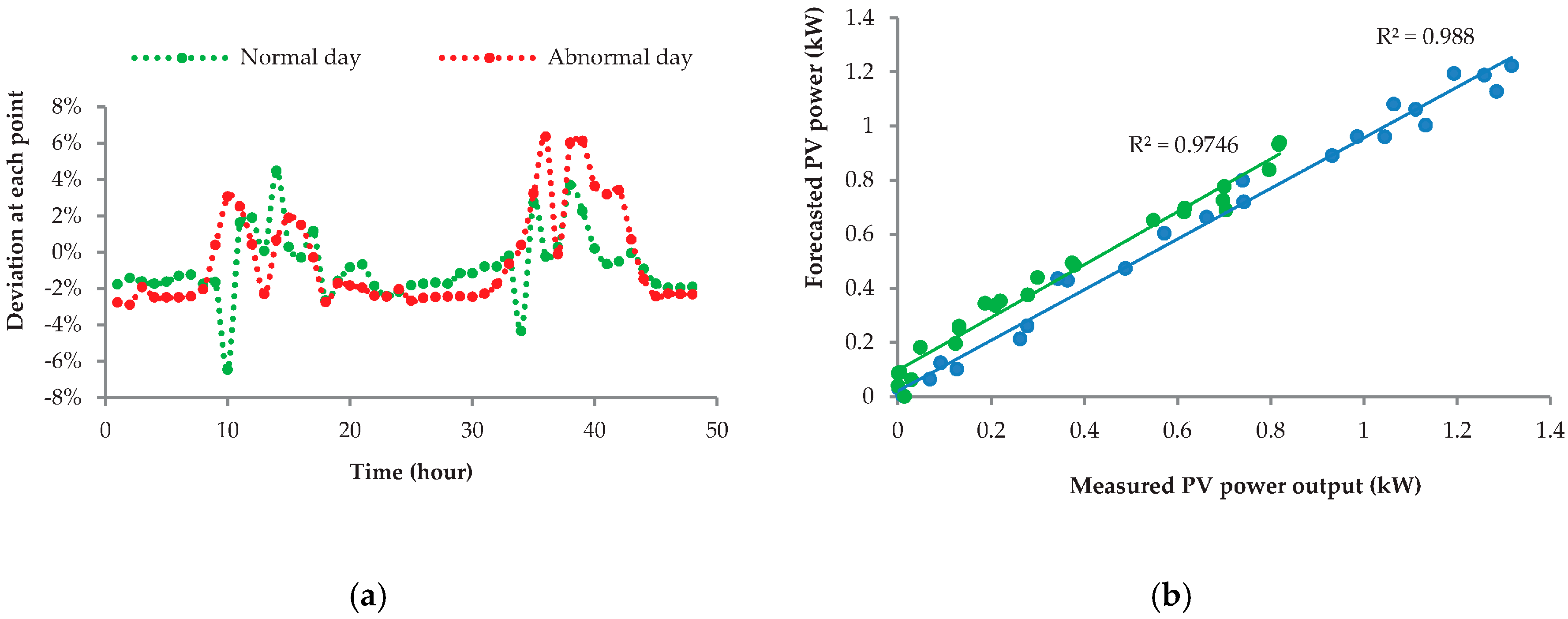
Figure 9a shows the deviation of the actual measured PV power output and the PV power output of the proposed forecasting model of plant-2 in different weather conditions. The deviation of the measured and forecasted PV power generation at each particular point was not higher than 10%, a percentage in the allowable range. The figure also shows that deviations in different weather conditions do not change drastically. The deviations for all plants were then evaluated on the basis of all datasets. In all cases, the results were almost similar to the deviation.

For the proposed model, Figure 9b shows the correlation of the actual measured PV power output and the forecasted PV power of plant-2 in different weather conditions. The correlation coefficient of $R^2=0.988$ in normal weather conditions and $R^2=0.9746$ in abnormal weather conditions explains the intensity of the correlation; that is, the correlation between the measured power and the forecasted power is very good. The positive sign of this value expresses the proportional relationship between the two powers. Based on this analysis, the proposed model performs very well.

5. Conclusions

Accurate forecasting of PV power generation has become a key point in the reliable operation of electrical grids due to the related rapid connection of PV systems to the grid. In this study, a generalized SVR-based forecasting model was proposed to accurately forecast PV power generation in different weather conditions. The proposed model was applied to three different PV power stations, and then its performance was analyzed. The generalized model could forecast PV power generation in both normal days (clear-sky) and abnormal days (cloudy or rainy days) with nearly the same accuracy. The proposed model could also accurately forecast PV power generation in various seasonalities and different abnormal weather conditions. Deviations in the actual measured and forecasted PV powers at each particular point were in an acceptable range (i.e., not greater than 10%), and no drastic fluctuations at any point were observed. The correlation between the actual measured PV power and the forecasted PV power for the proposed model was also very good. Subsequently, this simple model could significantly reduce computational complexity yet increase model accuracy. The model was experimentally validated by deploying it to three different types of PV plants in the same location. The average forecasting errors of the model were 3.08% in nRMSE, 34.57 W in MAE, and 11.34 W in MBE. Finally, the proposed model outperformed the ANN model, the persistence model, and other conventional models.