Numerical Analysis of Flatback Trailing Edge Airfoil to Reduce Noise in Power Generation Cycle

Abstract

Turbo machinery is an essential part in the power generation cycle. However, it is the main source of noise that annoys workers and users, and contributes to environmental problems. Thus, it is important to reduce this noise when operating the power generation cycle. This noise is created by a flow instability on the trailing edge of the rotor blade—an airfoil that becomes a section of the rotor blade of the rotating machine—manufactured as a blunt trailing edge (T.E.), with a round or flatback shape, rather than the ideal sharp T.E. shape, for the purposes of production and durability. This increases the tonal noise and flow-induced vibrations at a low frequency, owing to vortex shedding behind T.E. when compared with a sharp T.E. In order to overcome this problem, the present study investigates the oblique T.E. shape using numerical simulations. In order to do so, flow was simulated using large eddy simulation (LES) and the noise was analyzed by acoustic analogy coupled with the LES result. Once the simulation results were verified using the flatback airfoil measurements of the Sandia National Laboratories, numerical prediction was performed to analyze the flow and the noise characteristics for the airfoils, which were modified to have oblique trailing edge angles of 60°, 45°, and 30°. From the simulation results of the oblique T.E. airfoil, it could be seen that the vortex shedding frequency moves in accordance with the oblique angle and that the vortex shedding noise characteristics change according to the angle, when compared to the flatback T.E. airfoil. Therefore, it is considered that modifying the flatback T.E. airfoil with an appropriate oblique angle can reduce noise and change the tonal frequency to a bandwidth that is suitable for mechanical systems.

1. Introduction

A compressor and a turbine are essential components in the power generation cycle, such as the Rankine or Brayton cycles. A compressor or a turbine creates high-level noise that annoys users and causes environmental issues. Sometimes, the compressor operates under the designed speed to reduce overall noise level [1]. This reduced operating speed has a negative effect on efficiency and performance. For this reason, the reduction of noise is one of the essential problems for compressor and turbine operation in the power generation cycle. The main source of noise of these machines is aerodynamic noise produced by the rotor, screw, impeller or nozzle [2,3]. Thus, it is necessary to improve noise levels using a geometric design for the airfoil and the blade.

Airfoil shape—which is the sectional geometry of the blade—is an important design consideration, not only for the fixed wings of an aircraft, but also for a variety of rotating machines, such as compressors, turbines, pumps, propellers, and rotor blades [4,5]. Ideally, the trailing edge (T.E.) of an airfoil requires a sharp shape with a thickness of zero. However, practically, it is not easy to maintain a sharp trailing edge shape because of the issues associated with damage during manufacturing and operation. In particular, a flatback airfoil is applied to increase sectional stiffness in the case of a heavy-weighted blade or high loading. Therefore, an airfoil is manufactured with a blunt T.E. in a round or flatback shape for the blades of some rotating machines (Figure 1) [6,7,8,9,10]. The main advantage of a blunt T.E. in the blade root of a rotating machine is to increase the structural strength, owing to the increased cross-sectional area and a second load path [11,12,13]. It could cause sectional stiffness increases through additional structures and can also increase the sectional area. For this reason, a thick flatback airfoil was applied to the inner region, near the hub of the large turbine blade [11].

However, an airfoil with a blunt or flatback T.E. shape increases pressure drag and tonal noise component at low frequencies [14,15,16]. When airfoils with a blunt or flatback T.E. shape are employed in turbines and compressor rotors, such tonal noise may act as one of the main noise sources [17,18]. This tonal noise is associated with the ringing of coherent structures near the trailing edge and involves the unsteady behaviors of counter-rotating stream wise vortices that are related to Karman vortex streets [19]. Such unsteady three-dimensional characteristics are related to the Reynolds number, turbulence intensity of the free stream flow, and the turbulence components in the boundary layers near the T.E. [20]. In addition, the wake, due to vortex shedding in the case of blunt T.E.s, may, not only result in resonance in turbines and compressor rotor blades, but also cause structural problems in multi-stage compressors or turbines, because they can make an unsteady loading in the next-stage blade [21,22,23]. Moreover, for cogwheel screw compressors, the tip cannot be manufactured with a sharp shape and potentially acts as a source of noise or vibration.

Many studies have been carried out to explain the physical phenomena and to find a prediction model of this tonal noise. Brooks and Hodgson [24] measured and suggested some models for blunt and sharp T.E. airfoil noise. Blake and Gershfeld [25,26] showed that T.E. vortex shedding was pronounced on both symmetric and blunt T.E. geometries in their experiments. Prasad and Williamson [27] reviewed vortex dynamics that were related to the wakes of a bluff body. Shannon and Morris [28] measured the wake behind blunt trailing edge by using particle image velocimetry (PIV) technique. Huerre and Monkewitz [29] also provided flow instability and wake flow of a bluff body. However, at present, despite many studies, a complete description of this tonal noise phenomenon is still missing. This is partly owing to the limitations and shortcomings of classical hydrodynamic stability theory. For instance, spatial stability analyses correctly predict the frequency of the most dominant tone [30], but they are unable to predict the tonal noise of an airfoil for a complex T.E. geometry. In addition, some studies have attempted to reduce this tonal noise. In an experimental study of flatback airfoils, Berg and Zayas [31] designed a flatback root blade section with a thickness to chord length ratio of 0.1 and performed aerodynamic and acoustic tests in a wind tunnel. Kim et al. [32,33] performed numerical simulation of flatback airfoil aerodynamic noise using hybrid reynolds-averaged navier stokes equations – large eddy simulation (RANS-LES) and acoustic analogy. They also predicted blunt T.E. vortex shedding noise by introducing a modified empirical formula. In another study, an attachment was fixed on the T.E. for noise reduction [34]. Barone et al. [35] reduced flatback airfoil noise by 4 dB using a splitter plate that was attached to the blunt T.E. In their numerical studies of blunt T.E. airfoils, Stone et al. [36] achieved a 5 dB noise reduction at a 5° angle of attack by attaching a splitter plate behind the flatback wing; however, no experimental validation was reported. Although attachments, such as splitters, may reduce noise, they complicate the blade manufacturing process and reduce service life. Therefore, there is a need for a T.E. shape treatment that considers production, while reducing noise.

Toward this end, an oblique T.E. coupled with flatback geometry is considered to maintain the structural advantage of the flatback T.E. shape and also reduce tonal noise. An appropriately shaped oblique T.E. may weaken the vortex shedding phenomenon at the lower surface and break the vortex street behind T.E. Furthermore, oblique T.E. may eliminate tonal noise by reducing the interference via vortex offsetting and changing the frequency that generates flow-induced vibrations. As mentioned before, although there have already been many experiments and research on airfoil T.E. noise, it is still difficult to predict the T.E. tonal noise of complex flatback T.E. geometry with previous models [37]. Thus, in this study, a numerical approach was used to consider the T.E. geometry effect of flatback airfoil in the reduction of tonal noise and wake instability.

T.E. flow, and the noise generated by a T.E., cannot be analyzed using the Reynolds-Averaged Navier Stokes (RANS) equation because of accuracy problems [36]. For computational aero-acoustics (CAA) using the direct numerical simulation (DNS) method, accurate noise predictions can be expected, albeit with a significant increase in computing requirements because a very fine mesh and a highly accurate scheme are required with regard to time and space [38,39]. In the present work, the large eddy simulation (LES) model and the Ffowcs Williams-Hawkings (FW-H) acoustic analogy model were used to capture the wake instabilities and to predict the radiated noise made by a flatback T.E. Large eddy simulation is a useful tool for general realistic turbulence problems. To reduce the calculation time, steady-RANS results were used for the initial condition of the transient-LES calculation. The radiated sound was obtained using the FW-H model to predict dipole noise by pressure fluctuations on the airfoil surface.

The main objective of using the flatback T.E. shape airfoil is to increase sectional stiffness in the root region. A thick airfoil is applied to the inboard section near the hub (r/R < 20%), especially in large turbine blades, to ensure sufficient structural safety [40]. In addition, instead of applying an additional secondary spar structure, the trailing edge region of the flatback airfoil was utilized as a load dispersion structure to resolve a buckling problem [41]. Furthermore, an overall aerodynamic performance of the rotating blade was less affected by the sectional lift coefficient inboard region. Thus, aerodynamic performance is relatively less important at the inboard section of the rotating machine.

For this reason, the oblique angle was selected in this study, as noise and structural sectional stiffness were considered as the objectives. Less oblique angles may make less noise but have a low sectional stiffness. The modified T.E. shape can decrease airfoil lift. At the inboard region, however, the sectional stiffness is more important than the lift coefficient. Thus, it is important to find an oblique angle that is as large as that of the large sectional stiffness, but one that has lower noise levels.

In this study, primarily, the accuracy of the numerical results was verified using the analysis method described above—the noise measurement data [35] of the DU97W300 flatback airfoil, which was tested by the Sandia National Laboratories. Subsequently, to reduce the tonal noise of the flatback T.E. airfoil, T.E. was modified with an oblique shape, and the effects were analyzed using numerical simulations.

2. Methodology

2.1. Large Eddy Simulation

The objective of this paper is to simulate a blunt T.E. vortex shedding noise that is induced by external flow. The fluid has Newtonian flow characteristics, such that the shear stress is proportional to the rate of change. This flow can be governed by the Navier-Stokes equation. The Navier-Stokes equation consists of five main equations, including one continuity equation, three momentum equations, and one energy conservation equation (Equations (1)–(3)).

$$\frac{\partial }{\partial t}\left({\int }_V\rho dV\right)+{\oint }_A\rho v·da={\int }_{V}SdV,$$

(1)

$$\frac{\partial }{\partial t}\left({\int }_V\rho vdV\right)+{\oint }_A\rho v\otimes v·da=-{\oint }_{A}pI\cdot da+{\oint }_{A}T\cdot da+{\int }_V{f}_{b}dV,$$

(2)

$$\frac{\partial }{\partial t}\left({\int }_V\rho EdV\right)+{\oint }_A\rho Hv\times da=-{\oint }_A{\dot{q}}^{″}\cdot da+{\oint }_{A}T\cdot vda+{\int }_V{f}_b·vdV+{\int }_V{S}_{E}dV,$$

(3)

where p, ρ, I, T, and f_b denote the pressure, density, identity tensor, stress tensor, and body force, respectively. Every velocity component is included in vector v.

The wake is the major noise source of blunt trailing edge airfoils. Thus, an accurate turbulence model is usually necessary in this case. For this reason, the LES turbulence model was applied to this numerical simulation. LES involves large-scale analysis of turbulence, while the small-scale eddy is a modelling method. In contrast to the RANS equations, the equations that are used to solve large eddy simulations are obtained using spatial filtering rather than an averaging process. Each solution variable $\varnothing$ (velocity compoents, pressure, and so on) is decomposed into a filtered value $\tilde{\varnothing }$ and a sub-filtered, or sub-grid, value ${\varnothing }^{\prime }$ as:

$$\varnothing =\tilde{\varnothing }+{\varnothing }^{\prime },$$

(4)

The filtering of the generic instantaneous flow variable $\varnothing \left(t,x\right)$ is defined as:

$$\tilde{\varnothing }\left(t,x\right)={\int \int \int }_{-\infty }^{\infty }G\left(x-x^{\prime },\Delta \right)\varnothing \left(t,x^{\prime }\right)d{x}^{\prime },$$

(5)

where $G\left(\mathit{x},\Delta \right)$ is a filter function that is characterized by a filter with $\Delta ={\left({\Delta }_x{\Delta }_y{\Delta }_z\right)}^{1/3}$.

The filtered Navier-Stokes equation, expressed in Cartesian coordinates, can be expressed as Equations (6) and (7):

$$\frac{\partial \rho }{\partial t}+\nabla \times \left(\rho \tilde{v}\right)=0,$$

(6)

$$\frac{\partial }{\partial t}\left(\rho \tilde{v}\right)+\nabla \times \left(\mathsf{\rho }\tilde{v}\otimes \tilde{v}\right)=-\nabla \times \tilde{p}I+\nabla \times \left(T+T_t\right)+f_b,$$

(7)

where $\tilde{v}$ and $\tilde{p}$ are the filtered velocity and pressure, respectively.

Based on the eddy-viscosity model [42] of Boussinesq, the tensor is modelled as:

$$T_t=2{\mu }_{t}S-\frac{2}{3}\left({\mu }_t\nabla \times \tilde{v}+\rho k\right)I,$$

(8)

where S is the mean strain rate tensor and k is the sub-grid scale turbulent kinetic energy.

As a sub-grid scale model, the wall-adapting local-eddy (WALE) [43] sub-grid scale model was applied.

As for the spatial scheme, the third-order central difference Monotonic Upstream-Centered Scheme for Conservation Laws (MUSCL) scheme was blended as the convection scheme in spatial discretization. The upwind blending factor was 0.15 and MinMod was used as a gradient limiter. As for the temporal scheme, a second-order temporal scheme was applied. A second-order temporal scheme discretization of the unsteady term uses the solution at the current time level, n + 1, as well as the solutions from the previous two time levels, n and n − 1, as follows:

$$\frac{d}{dt}{\left(\rho \chi \varphi V\right)}_0=\frac{\left\{\left({\alpha }^2-1\right)\left[{\left(\rho \chi \varphi V\right)}_0^{n+1}-{\left(\rho \chi \varphi V\right)}_0^n\right]+\left[{\left(\rho \chi \varphi V\right)}_0^{n-1}-{\left(\rho \chi \varphi V\right)}_0^n\right]\right\}}{\alpha \left(\alpha -1\right)\mathsf{\Delta }{t}^{n+1}}$$

(9)

and:

$$\mathsf{\alpha }=1+\frac{\mathsf{\Delta }{t}^{n+1}}{\mathsf{\Delta }{t}^n}$$

(9a)

$$\mathsf{\Delta }{t}^{n+1}=t^{n+1}-t^n$$

(9b)

$$\mathsf{\Delta }{t}^n=t^n-t^{n-1}$$

(9c)

where χ is the void fraction. In the air case, χ is 1, $\varphi$ is the scalar quantity and V is the cell volume.

On the first time-step of the second-order temporal simulation, the first-order discretization was used since only two time levels were available.

2.2. Acoustic Analogy

Noise prediction was performed using the Ffowcs Williams-Hawkings (FW-H) equation [25]. This model calculates the far-field noise that is radiated from the near-field data of the computaional fluid dynamics (CFD) result. The FW-H formulations are based on Farassat’s formulation 1A, which is an extension of Lighthill’s acoustic analogy [44]. Farassat’s formulation 1A is a non-convective form of FW-H for general subsonic source regions, which includes the impermeable formulation. In this study, the impermeable surface that coincided with the airfoil surface was applied for surface integration because the tonal noise of the blunt T.E. airfoil was generated by vortex shedding at the airfoil T.E. [45].

The FW-H equation is an exact rearrangement of the continuity and the momentum equations into the form of an inhomogeneous wave equation. The FW-H equation gives accurate results, even if the surface of integration lies in the nonlinear flow region. The equation is based on the free-space Green’s function to compute sound pressure at the observer location, x. The FW-H equation for the pressure that is radiated into a medium at rest by a flow in a region or a set of surfaces is:

$${\mathrm{p}}^{\prime }\left(x,t\right)={{\mathrm{p}}^{\prime }}_T\left(x,t\right)+{{\mathrm{p}}^{\prime }}_L\left(x,t\right)+{{\mathrm{p}}^{\prime }}_Q\left(x,t\right),$$

(10)

The monopole, dipole, quadrupole terms are:

$${{\mathrm{p}}^{\prime }}_T\left(x,t\right)=\frac{1}{4\pi }\left(\left(\frac{\partial }{\partial t}\right)\right){\int }_S{\left[\frac{Q}{\left(r\left(1-M_r\right)\right)}\right]}_{ret}dS,$$

(11)

$${{\mathrm{p}}^{\prime }}_L\left(x,t\right)=\frac{1}{4\pi }\left(\left(-\frac{\partial }{\partial x_i}\right)\right){\int }_S{\left[\frac{L_i}{\left(r\left(1-M_r\right)\right)}\right]}_{ret}dS,$$

(12)

$${{\mathrm{p}}^{\prime }}_Q\left(x,t\right)=\frac{1}{4\pi }\left(\left(\frac{{\partial }^2}{\left(\partial x_i\right)\left(\partial x_j\right)}\right)\right){\int }_V{\left[\frac{T_{ij}}{\left(r\left(1-M_r\right)\right)}\right]}_{ret}dS,$$

(13)

with:

$$Q={\rho }_0\left(\left(1-\frac{\rho }{{\rho }_0}\right)v_i+\frac{\rho u_i}{{\rho }_0}\right),$$

(14)

$$L_i=\left(\left(p-p_0\right){\delta }_{ij}-{\sigma }_{ij}\right)n_i+\rho u_i\left(u_n-v_n\right),$$

(15)

$$T_{ij}=\rho u_i{u}_j+{\delta }_{ij}\left[\left(p-p_0\right)-c_0^2\left(\rho -{\rho }_0\right)\right]-{\sigma }_{ij},$$

(16)

where: $u_i$ and $v_i$ are the fluid velocity component in the $x_i$ direction. $u_n$ and $v_n$ are the fluid velocity component normal to the surface. $n_i$ is the viscous stress tensor and ${\rho }_0$ is the far-field density.

The space derivatives from Equations (11) and (12) are transformed into time derivatives. Afterwards, the time derivatives at the observer locations are moved into the integrals.

When the integration surface coincides with the body, the total surface term, ${\mathrm{P}}^{\prime }{}_S\left(x,t\right)$, is the result of the sum of the thickness surface term and the loading surface term:

$${\mathrm{P}}^{\prime }{}_S\left(x,t\right)={\mathrm{P}}^{\prime }{}_T\left(x,t\right)+{\mathrm{P}}^{\prime }{}_L\left(x,t\right),$$

(17)

Farrassat’s formulation 1A is for general subsonic source regions and for a general far-field noise prediction [46,47]. This formulation is shown in Equations (18) and (19).

$${\mathrm{P}}^{\prime }{}_T\left(x,t\right)=\frac{1}{4\pi }\left({\int }_{\left(f=0\right)}{\left[\frac{{\rho }_0\left({\dot{U}}_n+U_{\overline{n}}\right)}{r{\left(1-M_r\right)}^2}\right]}_{ret}dS+{\int }_{\left(f=0\right)}{\left[\frac{{\rho }_0{U}_n\left[r{\dot{M}}_r+a_0\left(M_r-M^2\right)\right]}{r^2{\left(1-M_r\right)}^3}\right]}_{ret}dS\right),$$

(18)

$${\mathrm{P}}^{\prime }{}_L\left(x,t\right)=\frac{1}{4\pi }\left(\frac{1}{a_0}{\int }_{\left(f=0\right)}{\left[\frac{{\dot{L}}_r}{r{\left(1-M_r\right)}^2}\right]}_{ret}dS+{\int }_{\left(f=0\right)}{\left[\frac{\left(L_r-L_M\right)}{r^2{\left(1-M_r\right)}^2}\right]}_{ret}dS+ \frac{1}{a_0}{\int }_{\left(f=0\right)}{\left[\frac{L_r\left[r{\dot{M}}_r+a_0\left(M_r-M^2\right)\right]}{r^2{\left(1-M_r\right)}^3}\right]}_{ret}dS\right)$$

(19)

where:

$$L_i=\left(\left(p-p_0\right){\delta }_{ij}-{\sigma }_{ij}\right)n_i+\rho u_i\left(u_n-v_n\right),$$

(20)

$$M_i=U_i/a_0,$$

(21)

$$r=x_{observer}-y_{face},$$

(22)

$f=0$ represents the emission surface and is made in coincident with a body (airfoil surface) and an impermeable surface. If the data surface coincides with a solid surface, then the normal velocity of the fluid is the same as the normal velocity of the surface: $u_n=v_n$. In this case, Equations (18) and (19) correspond to the impermeable FW-H surface type.

The major task in evaluating the FW-H integrals is to account for the time lag between emission and reception times. The advanced time algorithm looks forward in time to see when the observer perceives the currently generated sound waves [48]:

• The procedure starts with a sequence of emission times (conveniently taken as the flow times).
• The source strengths are calculated (thickness surface noise and loading surface noise) at all source elements (faces of the integration surfaces) for a given emission time.
• The contributions of the sources are interpolated in the far-field time domain to build the sound signal.

The total sound pressure that the observer perceives consists of the contribution from all source elements. The sound pressure at the receiver is obtained by accumulating the arriving signals in time slots. The overall observer acoustic signal is found from the summation of the acoustic signal from each source element of the FW-H surface during the same source time.

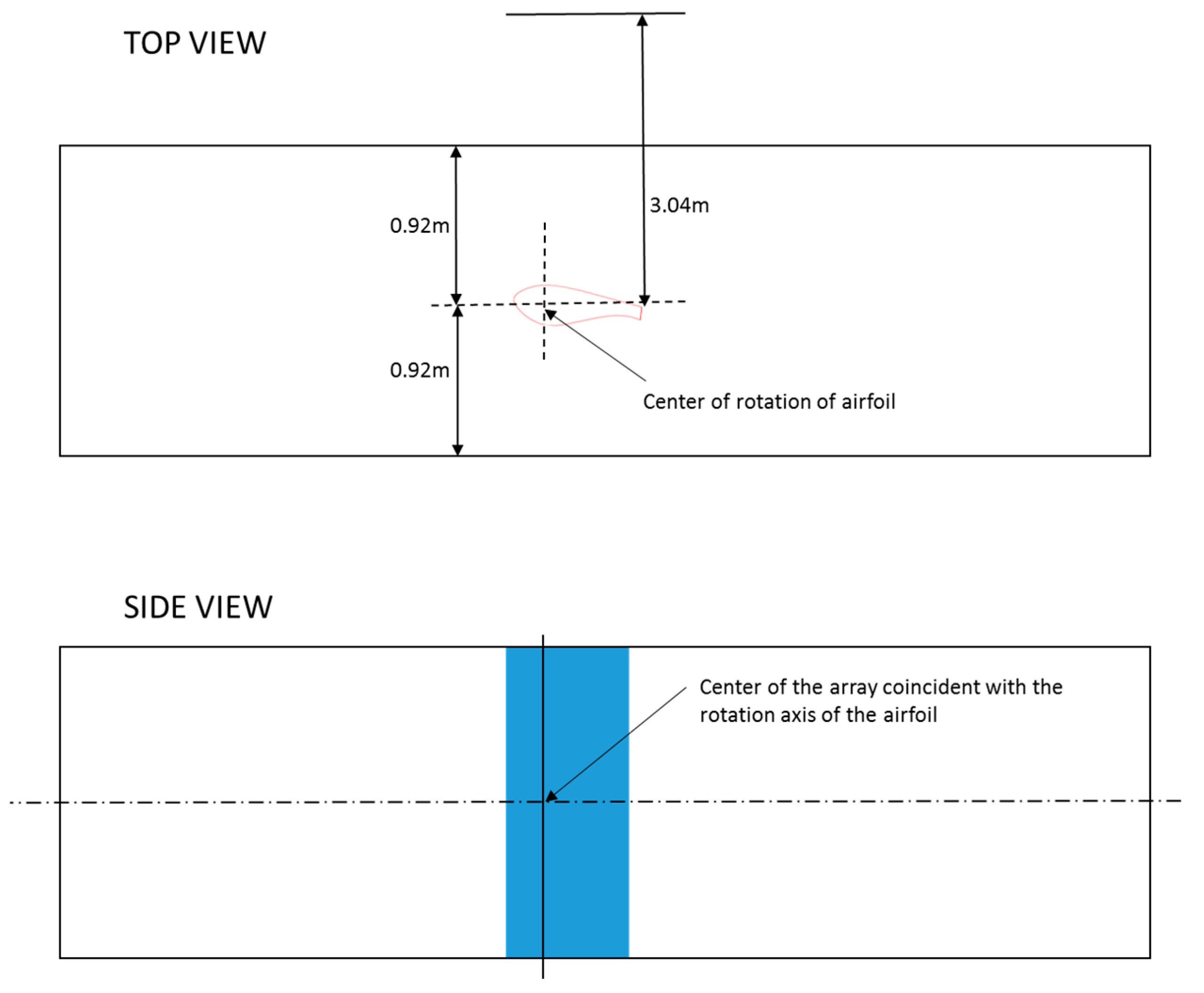
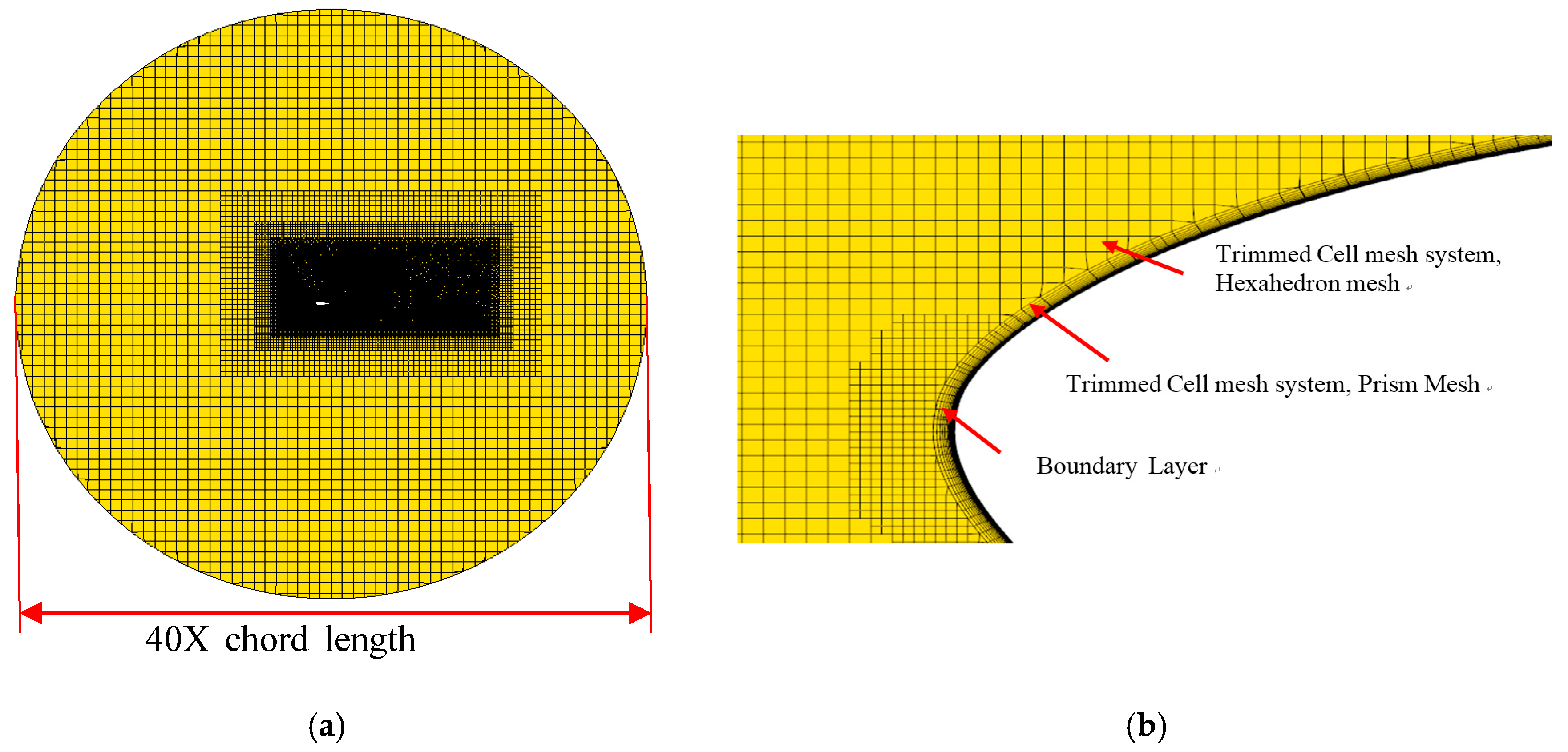
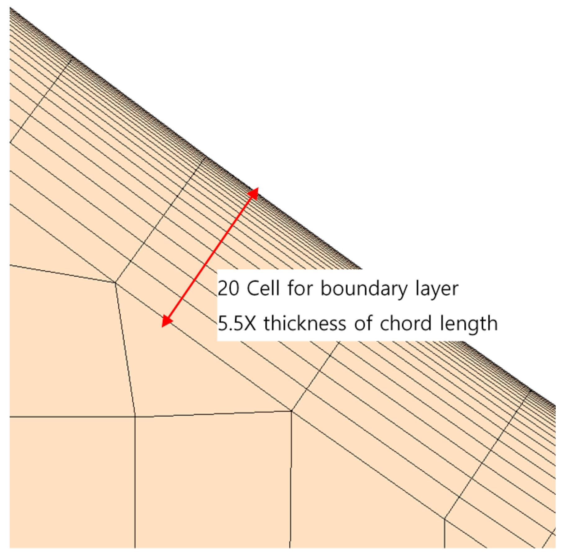
2.3. Numerical Conditions

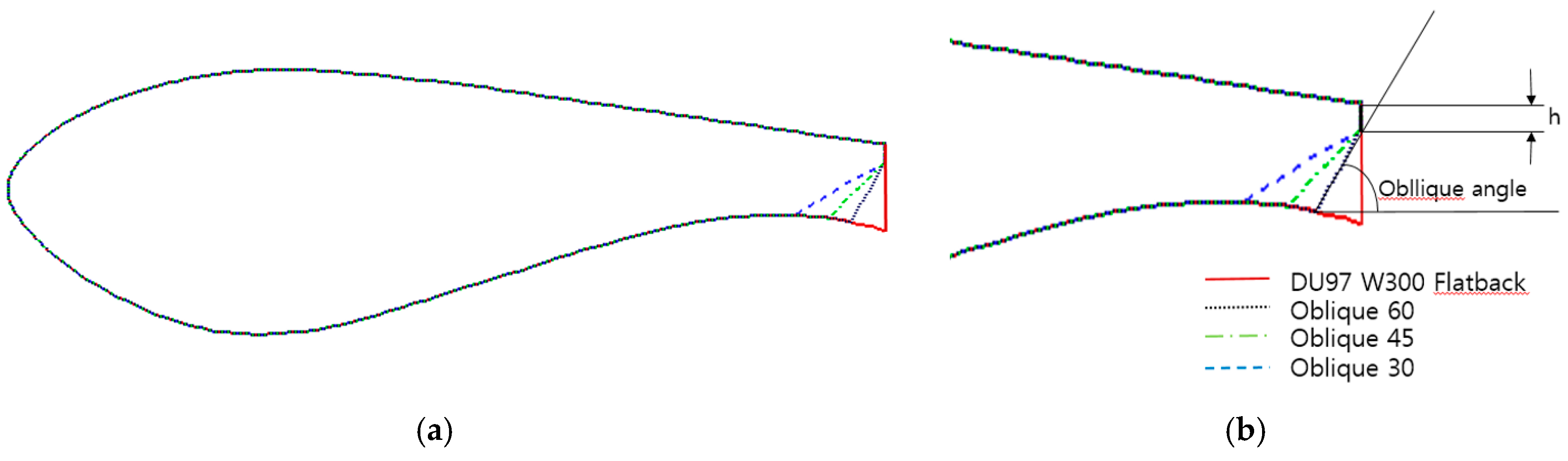
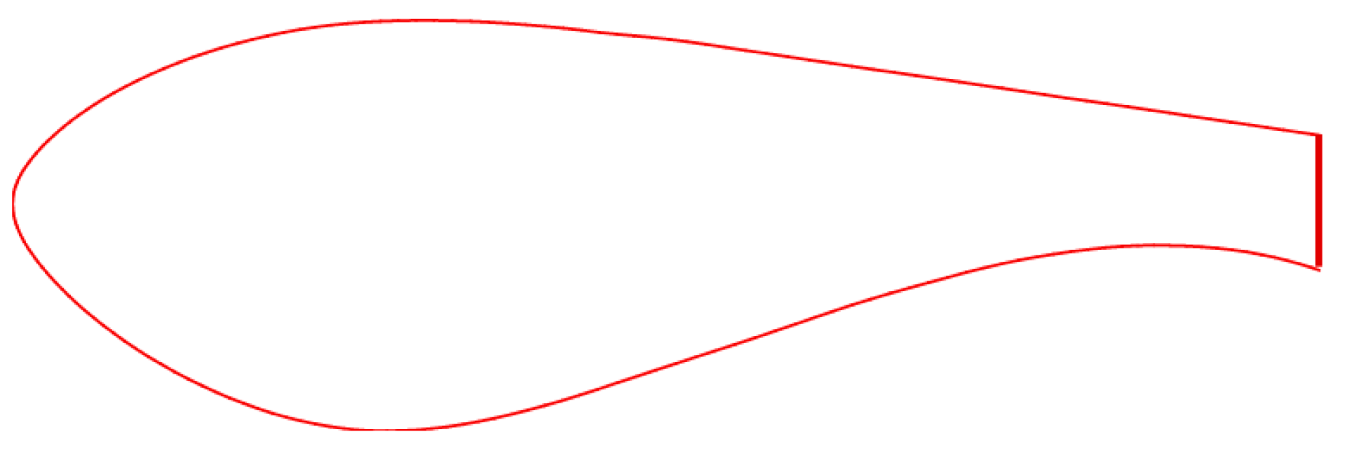
A commercial CFD S/W Star-CCM+ was used for the numerical simulation of noise analysis. For an accurate pressure fluctuation value in the time domain for noise analysis, LES was applied to the turbulence model while the results from the RANS model were used as the initial conditions for the LES model in order to shorten the calculation time.

For the grid resolution and structure for the CFD calculation, a grid system for LES model analysis was created, and the same grid system was applied to the RANS model. The entire calculation area was created as a circle, shown in Figure 2a, with a diameter of 40 times the chord length. The chord length of the CFD model was identical to that of the wind tunnel test model (0.91 m), while the length of the span was set to two times the chord length (1.82 m) in order to satisfy the LES grid criteria [49] suggested by Baggett. The basic grid structure is a trimmed cell mesh and was created as the block-structured grid type. The fluid region was created as a hexahedron mesh, and the area coming into contact with the boundary layer mesh was made with a prism mesh (Figure 2b). The area around the leading edge (L.E.), which is the stagnation point, has an alignment of cells created to be 0.275% of the chord length, forming a grid in which the cell size increases two-folds with the distance from the airfoil in a stepwise manner from 0.55% of the chord length to 70.4%. The boundary layer area was created by overlapping 20 layers in the normal direction on top of the airfoil surface. For a precise simulation of the boundary layer flow, the cell thickness in the first layer of the boundary layer area was set to 2.94 × 10⁻⁴ times the airfoil chord length, with a stretching factor of 1.2 so that the boundary layer was created until the 20 layers had a thickness of 5.5% of the chord length (Figure 3).

Table 1. The dx/dy in the prism layer mesh. dx: stream-wise direction, dy: surface normal direction.

Layer Number from the Surface Wall	Mid-Chord Region	Leading Edge Region
No.	dx/dy	dx/dy
1	186.7	93.3
2	155.6	77.8
3	129.6	64.8
4	108	54
5	90	45
6	75	37.5
7	62.5	31.3
8	52.1	26.1
9	43.4	21.7
10	36.2	18.1
11	30.2	15.1
12	25.1	12.6
13	20.9	10.5
14	17.4	8.7
15	14.5	7.3
16	12.1	6.1
17	10.1	5
18	8.4	4.2
19	7	3.5
20	5.8	2.9

shows the aspect ratio of each layer at the mid-chord region and the leading-edge region. At the leading edge, dx/dy fell below 30 from the 8th layer, and the thickness from surface to 8th layer was 0.049% of the chord length. At the mid chord region where the aspect ratio was the largest, dx/dy fell below 30 from the 12th layer. The thickness from the surface to the 12th layer was 1.1 × 10⁻³ of the chord length. In this case, pressure and velocity change in boundary layer normal direction were larger than the change in stream-wise direction. Thus, a large dx/dy did not result in a serious error. In addition, the aspect ratio near the leading edge was half of the other regions because pressure and velocity change in stream-wise direction was large in this region. Similar research by Mendonca, Kumar and Kim [50] used similar aspect ratio of dx/dy and showed the expected results. The aspect ratio of chord-wise to span-wise (dx/dz) was one. Figure 4 shows the surface mesh on the airfoil—they were built up to the external boundary, the same as the dx/dz ratio. The dx on the airfoil surface was 0.5% of airfoil’s chord length. The total mesh number was 17 million for each airfoil. Figure 5 shows the resulting y+ distribution on the surface of the airfoil after calculation was converged. Around the T.E. area where the vortex shedding occurs, the values are maintained under two. Figure 6 shows convective courant number contour that was calculated in the present mesh. Convective courant number was under 0.7 in most of the flow regions, except a few cells near the T.E. corner. It is considered that the present mesh quality was enough for the analysis.

In the turbulence model, the shear stress transport (SST) (Menter) K-omega model was applied for the RANS model to calculate the initial value for LES analysis [51]. In the LES model, the WALE model [43] was applied for the subgird-scale (SGS) model. Both the RANS model and the LES model used all of the y+ treatment methods as the wall function while the third-order MUSCL scheme was applied as the convection scheme in spatial discretization. As for the temporal scheme, a second-order temporal scheme was applied. In the LES model, the time discretization used 5.0 × 10⁻⁵ s intervals in the second order while simulation was conducted for 0.8 s for an adequate convection of vortex shedding flow in the T.E. for the condition with a chord length of 0.92 m and an inflow speed of 28.7 m/s.

The noise in the far-field caused by turbulence and arbitrary motion was calculated using the FW-H equation [25], based on Lighthill’s acoustic analogy [44].

2.4. Test Cases

The numerical analysis results were verified on the basis of a DU97-Flatback airfoil, used to examine the noise effects on airfoils having flatback and oblique T.E.s. After confirming the reliability of the applied method and calculation results by comparing the calculation results and the wind tunnel test results for the DU97-Flatback airfoil, the noise effects of the T.E. were analyzed by modifying the T.E. shape to oblique.

The DU97-Flatback airfoil is the flatback T.E. version of the DU97-W-300 airfoil, with the flatback shape of the T.E. being 10% of the chord length (Figure 7). The calculation results for this airfoil were compared with the measurement data obtained at the Virginia Tech Stability Wind Tunnel by Sandia National Laboratories [35]. The wind tunnel test model for the airfoil has a chord length of 0.914 m and a span length of 1.8 m. For validation of the aerodynamic results, the numerical results were compared with the Cp distribution on the surface of the airfoil that was measured under an effective angle of attack (AOA) of 4.4°, a flow speed of 28.7 m/s, a case of geometric AOA of 5.1°, and a flow speed of 58.6 m/s. For validation of the aero-acoustic result, the calculation results were compared with the results of the 1/12th octave band for the noise that was measured at a geometric AOA of 5.1° and a flow speed of 44 m/s (Re. No. = 2.4 × 10⁶). The measurement point was 3.04 m towards the suction side from the center of rotation of the airfoil.

In Sandia’s measurement, Porous wall interference correction method was applied because normal correction method was inadequate for a relatively thick airfoil such as DU97-Flatback airfoil [35]. This correction method showed an accurate result for Re. = 1.64 × 10⁶ but inaccuracy was increased as Re. No. was increased to Re. = 2.4 × 10⁶ or Re. = 3.2 × 10⁶. Our study focused on the reduction of tonal noise by vortex shedding between 100 Hz and 200 Hz. This tonal noise could not be seen in the Re. = 1.64 × 10⁶ case in Sandia’s measurement. In addition, the Re. = 1.46 × 10⁶ data has a poor S/N ratio because of background noise of the wind tunnel. However, Re. = 2.4 × 10⁶ data showed clear tonal noise and a good S/N ratio. Since our research target was to see the tonal noise reduction effect, an acoustic comparison for validation was implemented for Re. = 2.4 × 10⁶ despite there data being not corrected. Sandia’s report stated that the error might not be serious. For this reason, Re. = 1.64 × 10⁶ data were used for the validation of aerodynamic performance and Re. = 2.4 × 10⁶ data were used for noise analysis.

In order to examine the noise effects of the T.E. shape, numerical prediction was performed for a T.E. having a lower surface with an oblique shape, as shown in Figure 8. While maintaining 2% of the chord length for the flat portion of the T.E. so that the load path can be formed [52], the T.E. shape was created with slopes of 60°, 45°, and 30°. The definition of the oblique angle is shown in Figure 8b, and the comparison of the T.E. shape with the DU97W300 flatback airfoil is shown in Figure 8a. For this airfoil shape, the noise spectrum was compared by creating a grid and performing numerical analysis, as described in Section 2.3. As for the numerical analysis condition, the geometric AOA is 5.1° and the flow speed is 44 m/s (Re. No. = 2.4 × 10⁶), which is are the same conditions as the noise measurement.

3. Results and Discussion

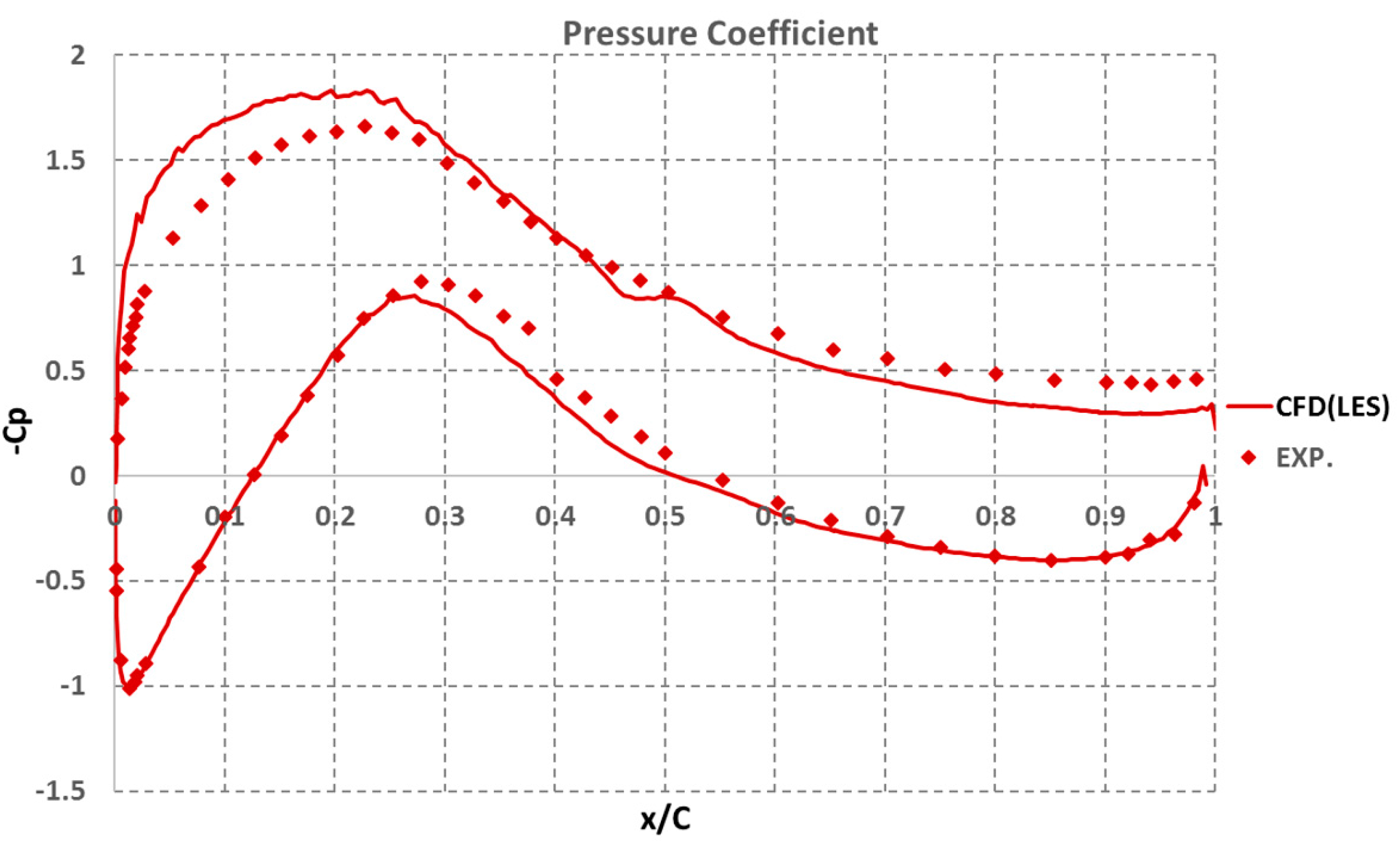
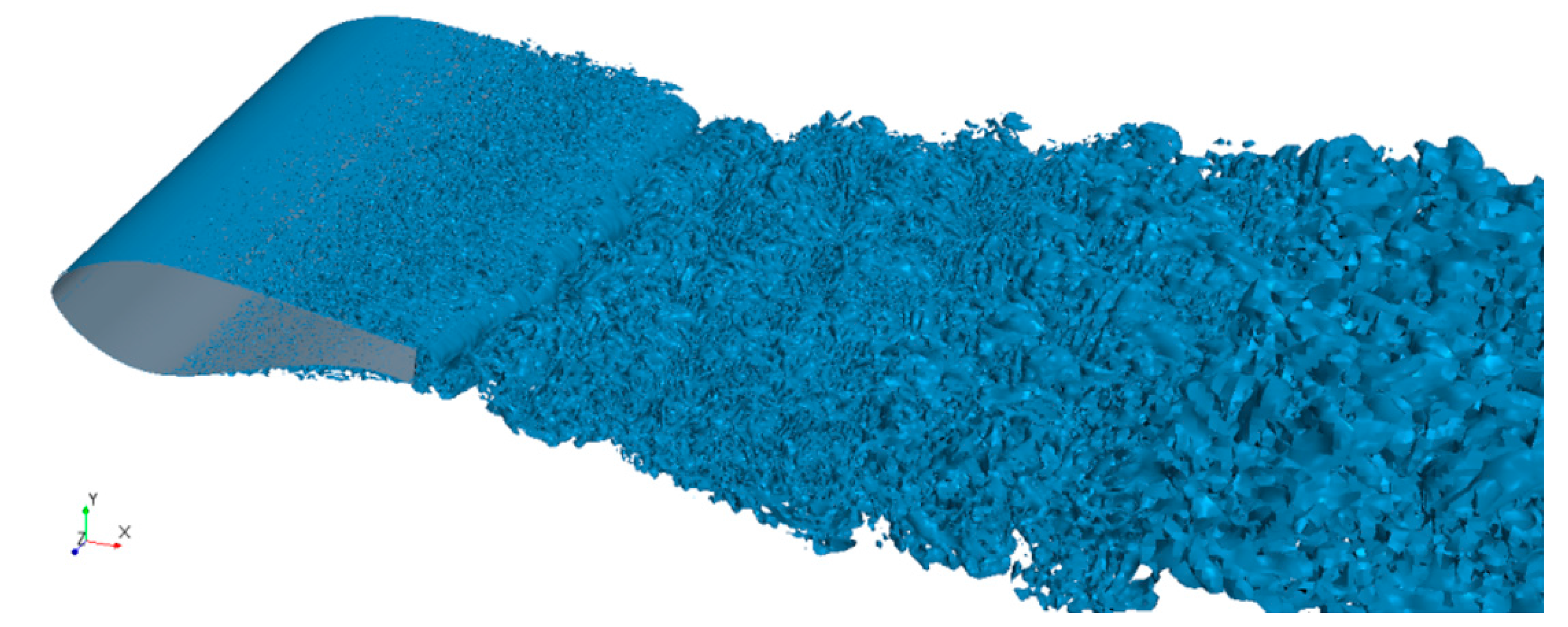
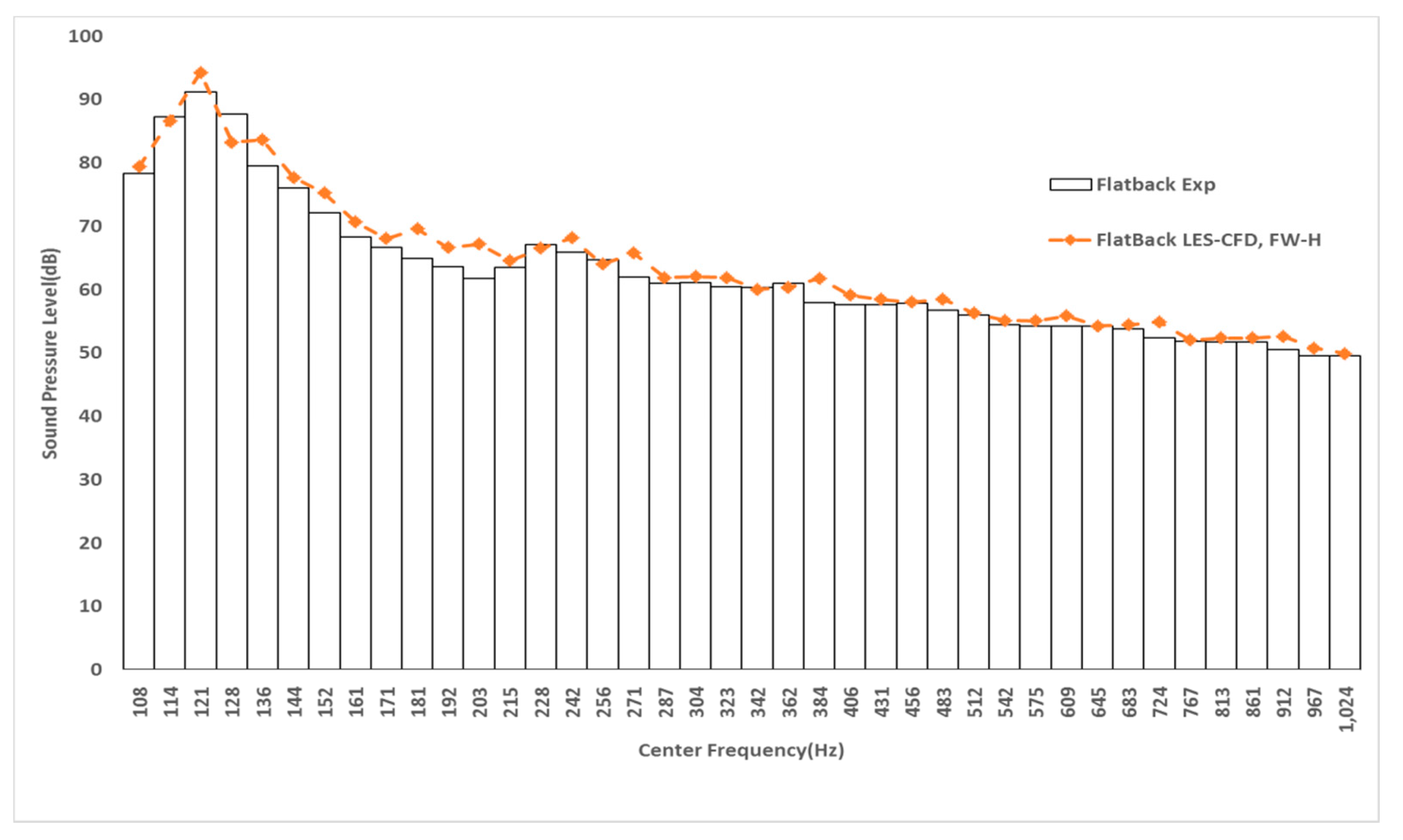
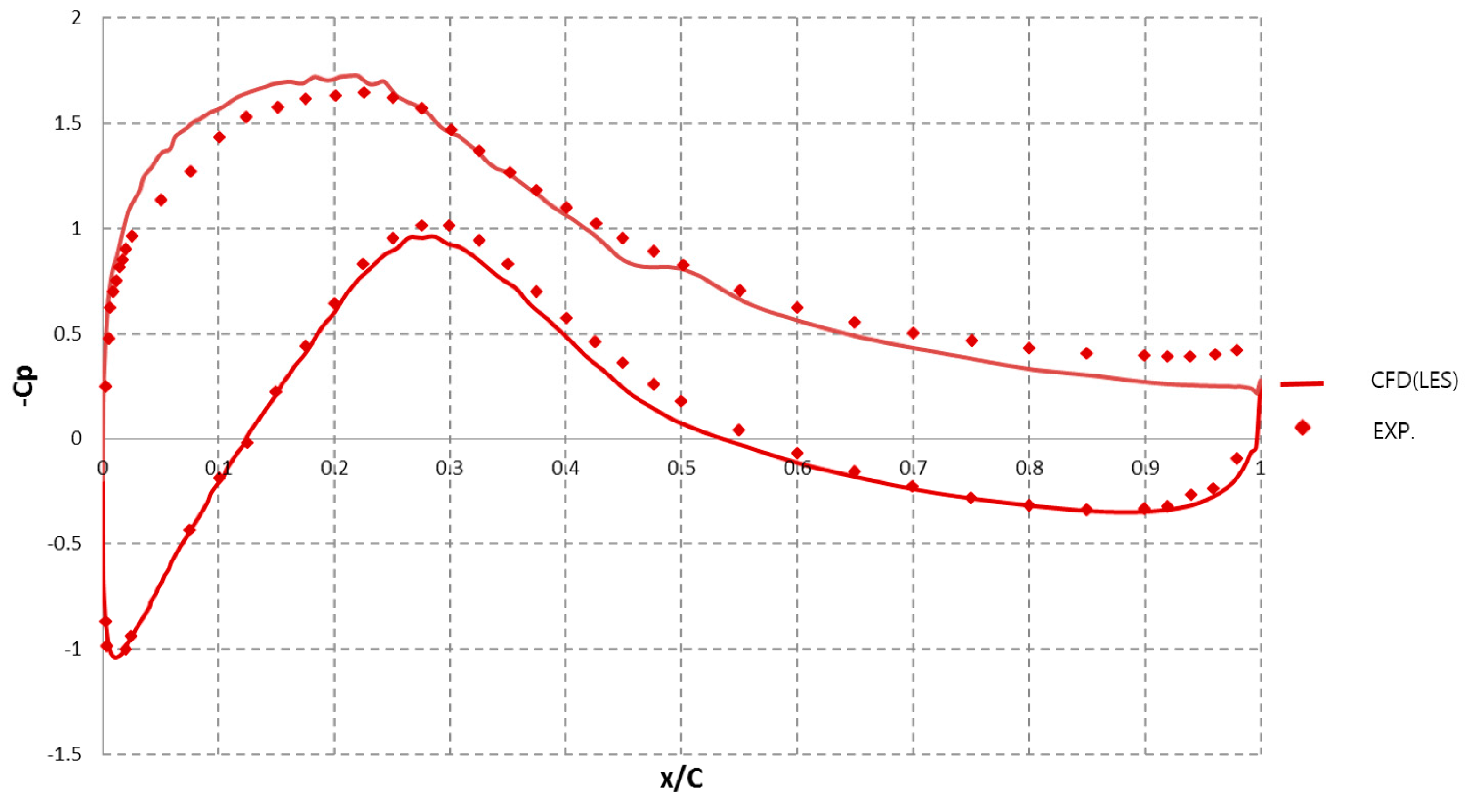
3.1. Validation of Aerodynamic and Aero-Acoustic Results

In order to verify the accuracy of the numerical results, a comparison was made with the untrip condition data [35] for the DU97-Flatback airfoil from the Sandia National Laboratories wind tunnel measurements.

For quantitative analysis of the aerodynamic simulation, the pressure coefficient was compared by conducting numerical analysis for an effective AOA of 4.4° with a flow speed of 28.7 m/s and Re. No. = 1.6 × 10⁶, and for a geometric AOA of 5.1° with a flow speed of 58.6 m/s and Re. No. = 3.2 × 10⁶. Here, the pressure coefficient (C_p) is defined as in Equation (23).

$$C_p=\frac{P-P_{\infty }}{\frac{1}{2}\rho U_{\infty }^2}$$

(23)

Figure 9 shows the C_p distribution and the comparison of the airfoil surface measured under ${\alpha }_{eff}=4.4°$, Re. No. = 1.6 × 10⁶. The x-axis shows the normalized chord length while the y-axis shows the –Cp values. In this case, the Sandia National Laboratories test results were corrected with an effective AOA of 4.4° while the CFD simulation was calculated by setting the geometric AOA = 4.4°. The overall CFD analysis results matched the test values well but show a slight difference with the L.E and T.E. regions of the upper surface. In the wind tunnel test, transition occurred from the laminar boundary layer to the turbulent boundary layer on the LE region, and such an error was the result of the fact that CFD analysis basically assumes full turbulent flow for the entire numerical domain. Therefore, slight over-prediction was observed for –C_p of the upper surface near the LE area compared to the experimental value, but the location of the apex was predicted relatively accurately, with values in the range of 20–25%.

Figure 10 shows the C_p distribution comparison of a geometric AOA of 5.1°, Re. No. = 3.2 × 10⁶. In the case of the Sandia National Laboratories test, the test conditions are not corrected by an effective AOA and only [35] geometric AOA is indicated; the same goes for noise measurements, which are described later, as they are also indicated in geometric AOA. Therefore, the AOA experienced by the airfoil in an actual test is smaller than 5.1°; as such, when the geometric AOA was calculated with a 5.1° in CFD analysis, the –C_p value in the upper surface turned out to be greater than the measured value, and the error also increased.

The qualitative overview of the flow can be seen in Figure 11 and Figure 12. Figure 11 shows the iso-surface of the Q = 100/s² value for the Q-criterion while Figure 12 shows the non-dimensional vortices contour. All calculation conditions are of geometric AOA of 5.1°, Re. No. = 2.4 × 10⁶, the same as the noise measurement condition. The vortices occurring in the boundary layer of the T.E. flow out to the back, creating a turbulent vortex street, and a visible wake pattern. The eddy created in the upper and lower surfaces convexed downstream, creating a 2D coherent structure, which also becomes the primary mechanism of generation for the vortex shedding noise in the case of a blunt T.E. [53]. Figure 11 and Figure 12 clearly show a trend similar to that of the results from the experiment by Shannon and Morris [28].

For the verification on noise analysis, a comparison was made with the data at a flow speed of 44 m/s, which clearly showed the components of tonal noise that were caused by the vortex shedding of the blunt T.E. For the angle of attack, for the reason previously mentioned, it was given a value in the Sandia report as the geometric angle of attack [35]. As the effective angle of attack is not accurately known, an AOA of 5.1° was used in the LES analysis as well as for comparison. Figure 13 shows the distribution of the Instantaneous Acoustic Pressure calculated using Equation (24) that were calculated from the CFD direct simulation. In this figure, the value of the acoustic pressure is large in the trailing edge and the vortex shedding area, which clearly shows that the main noise source of the tonal component is the vortex shedding at T.E.

$$\mathrm{Acoustic}\mathrm{Pressure}=P_{\mathrm{s},\mathrm{t}}- P_{\mathrm{average},\mathrm{calculation}\mathrm{time}}$$

(24)

Figure 14 shows the results of the 1/12th octave band noise comparison between the measurement and the numerical analysis. These were calculated by the acoustic analogy that was introduced in Section 2.2. The measurement point where the measurement and the calculation were compared is shown in Figure 15. This point was 3.04 m towards the suction side from the center of rotation of the airfoil.

In the anechoic system where the measurement was carried out, above 200 Hz and 0.610 m high, acoustic foam wedges eliminated acoustic reflections. Below 200 Hz, before the airfoil noise measurement, a correction factor was made by using the speaker and microphone measurements. The estimated corrections are less than 2 dB for frequencies greater than 100 Hz. These corrections gave confidence in the quality of the measured noise above 100 Hz. However, below 100 Hz, the estimated correction was between −4 dB and 6 dB. For this reason, noise was compared above 100 Hz. As for noise that is above 1000 Hz, a meaningful numerical result could not be calculated because FW-H coupled LES had limitation for broadband noise predication. Thus, the noise comparison was shown between 100 Hz and 1000 Hz in Figure 14.

The acoustic pressure signal that integrated along the whole airfoil surface in the numerical simulation (acoustic analogy) was explained in Section 2.2. For the measurement, the microphone array measured a selected area around the airfoil T.E. In this study, our main concerns were the tonal noise component by vortex shedding at T.E. This noise component is 20 dB higher than other noise. Thus, it was not considered a serious problem, despite the fact that the numerical calculation integrated the whole airfoil surface.

It can be seen that the numerical simulation’s result and measurement matched well. Overall, the numerical result is predicted to be 1–4 dB higher than the measurement; the reason for this is believed to be the angle of less than 5.1°—an effect of AOA of the airfoil in the actual wind tunnel test, which is the value used in the numerical analysis, resulting in a slightly higher numerical result compared to an actual measurement. In addition, as mentioned before, the numerical calculation integrated the whole airfoil surface but this measurement integrated only the T.E. area. However, both the numerical result and the measurement effectively showed the tonal noise components that were caused by the vortex shedding in the blunt T.E. at a bandwidth of 121 Hz, and the sound pressure level (SPL) values also matched well. The peak Strouhal number calculated with T.E. thickness, flow speed, and peak frequency is 0.251; this value also agrees well with the value suggested by Blake [53] and Brooks, Pope, and Marcolini [54].

As shown above, the numerical simulation result matched well with the measurement. This shows that the suggested numerical method yields reliable and significant results for aerodynamics and noise analysis using the blunt T.E. airfoil under the given conditions. Although there is an error between the geometric AOA and the effective AOA, the difference is negligible. As meaningful results can be obtained by comparing the noise caused by the T.E. geometry at the same AOA, numerical analysis according to T.E. geometry was performed for an AOA of 5.1° and Re. No. = 2.4 × 10⁶.

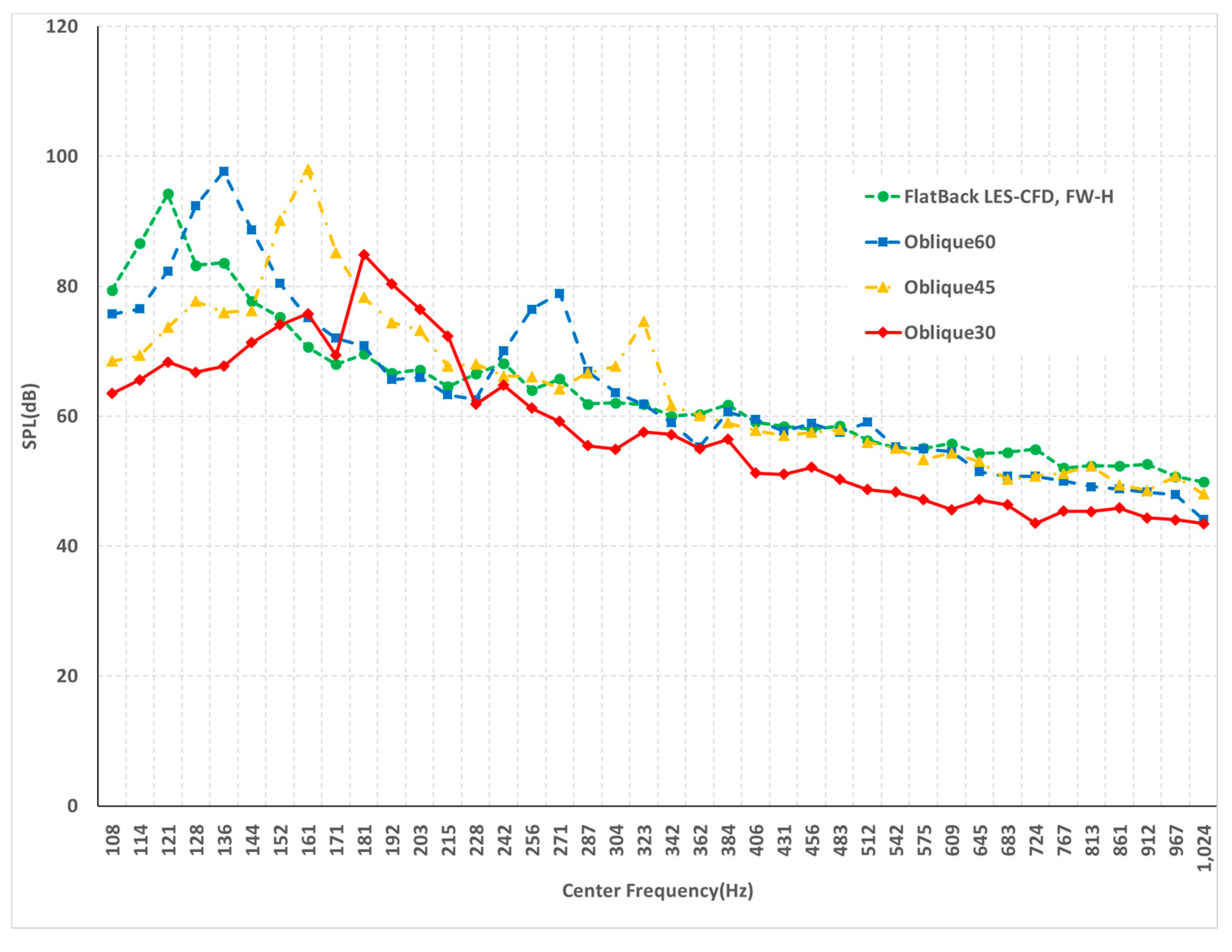
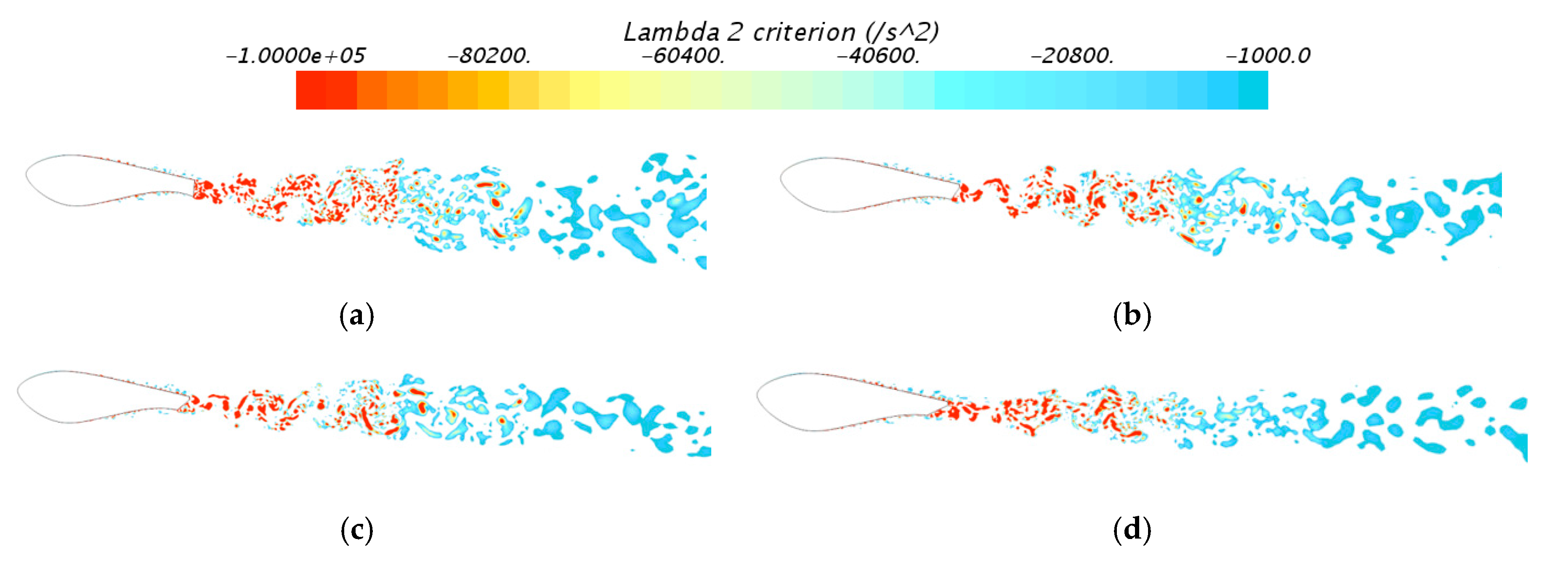
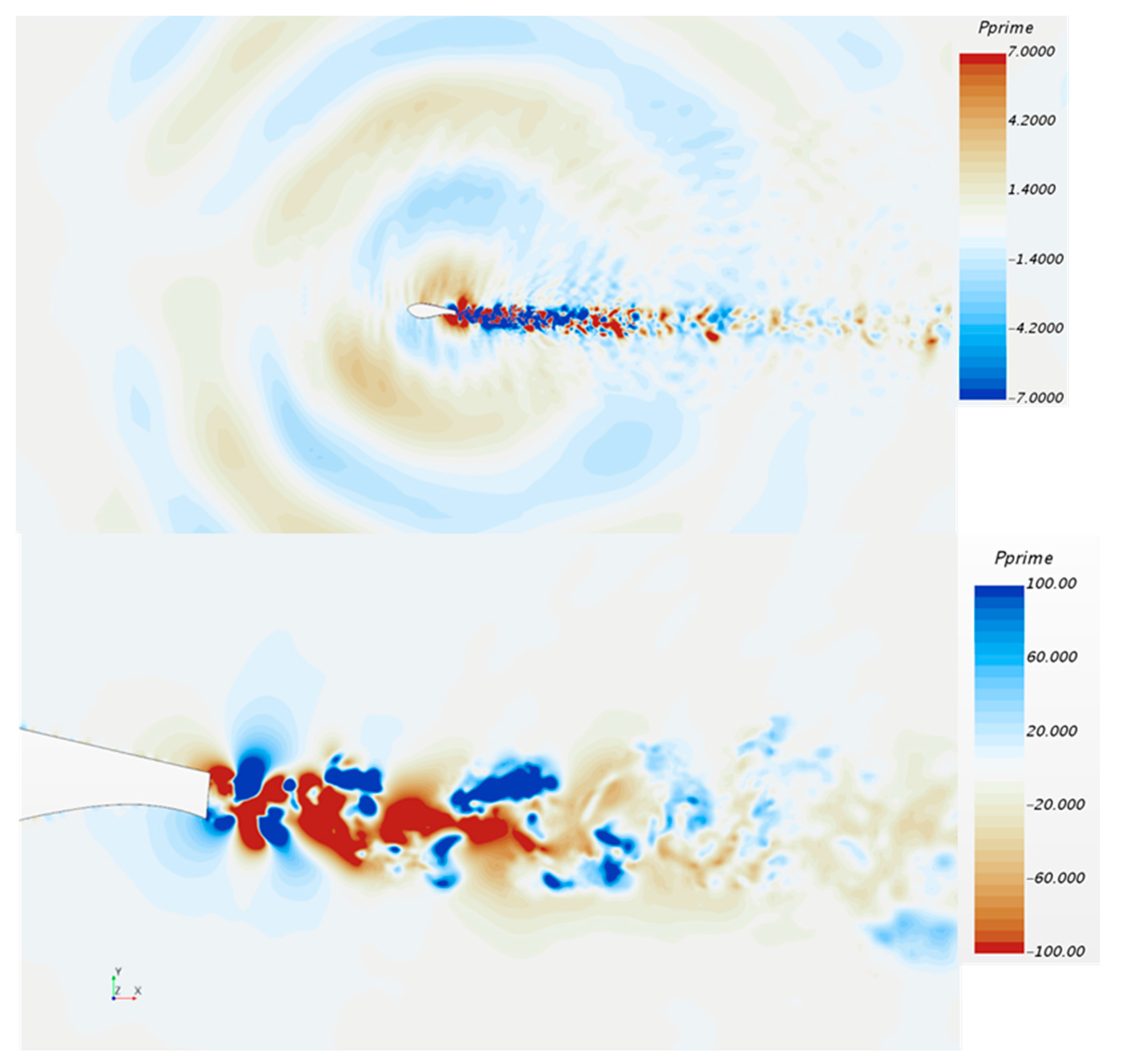
3.2. Noise Analysis of Oblique Trailing Edge Airfoils

As mentioned in Section 2.4, in order to reduce T.E. tonal noise by breaking the vortex street behind T.E., calculations were made by changing the oblique angle to 60°, 45°, and 30° while maintaining the flatback geometry to 2% of the chord length in the T.E. (Figure 8). In general, a high lift makes a high noise level and a sharp T.E. reduces the tonal noise level. As mentioned in previous sections, the objective of this study was to reduce the tonal noise level while maintaining the structural property as much as possible because sectional stiffness was more important than aerodynamic performance in the region where thick and flatback airfoil were applied. For this reason, a 2% flatback area was maintained for the loading path in the oblique T.E airfoils, and it was necessary to find the large oblique angle when a meaningful noise reduction was achieved.

Figure 16 shows the C_p distribution of each airfoil. Modification of the T.E. shape reduced C_p near T.E., and resulted in a decreased Cl (

Table 2. Sectional stiffness ratio, Cl, and tonal noise level of each airfoil.

Airfoil Name	Sectional Stiffness Based on Flatbak Airfoil (%)	Cl	Peak Noise Level (dB)
Flatback	100	0.98	94.2
Oblique60	95.8	0.79	97.7
Oblique45	94.6	0.72	97.9
Oblique30	93.6	0.66	84.8

). However, as for the peak tonal noise, noise level was maintained or slightly increased in the case of Oblique60 and Oblique45. This means that an improper oblique angle could reduce aerodynamic performance and structural property, and increase noise level.

Figure 17 shows the results of the noise comparison at 1/12th octave band for four T.E. shapes. When examining the frequency component, it can be seen that the tonal noise component frequency moves to the high frequency zone as flatback approaches Oblique30. Moreover, for Oblique30, only the main tonal noise component exists, and the second harmonic component is not really visible, but the second harmonic for the fundamental frequency is clearly visible for Oblique60 and Oblique45. This is because the cause of the harmonic component is the wake vortex street periodicity. It is considered that the spatially separated lower and upper vortices are made of distinct tonal noise, and the harmonics can be seen in Figure 18b,c. However, for Oblique30, the second harmonic component is weakened as the wake street of the vortex shedding breaks down earlier than that in the case of Oblique60 and Oblique45.

For SPL, the tonal noise level was nearly the same for Oblique60 and Oblique45, compared with the flatback T.E. airfoil. In comparison, for Oblique30, the tonal noise component was reduced significantly compared to the flatback T.E. airfoil. The cause can be determined upon examining the vortex shedding behind the airfoil trailing edge. Figure 18 shows the non-dimensional vortices contour and streamline around the airfoil T.E. For an airfoil with a flatback trailing edge shape, vortex shedding occurs strongly in the upper and lower surfaces. For Oblique60 and Oblique45 with oblique angles of 60° and 45°, respectively, the vortex shedding observed was similar to the case of the flatback airfoil in the upper and the lower surface of the T.E. However, these lower and upper vortices were separated distinctly in the spatial domain. Streamline clearly shows circulation in the upper side of the T.E. in these cases, as shown in Figure 18. Moreover, as the vortices convexed backward, they clearly showed separation from each other, and the tonal noise component increased compared to that of the flatback airfoil with a clear harmonic component. Vortex shedding noise is a dipole noise that is created by loading fluctuation on the airfoil surface. Figure 19 is a power spectral density of the drag coefficient that was calculated by the airfoil surface pressure. This figure shows clear tone and harmonics of Oblique60 and Oblique45.

For Oblique30, the coherent structure was destroyed as the vortex occurring in the upper surface and the weakening vortex shedding in the lower surface offset each other. In addition, Oblique30 reduces wake instability and make streamline smooth. It can be seen in the vertical velocity fluctuation behind T.E. Figure 20a shows the vertical velocity power spectral density along the chord behind T.E. The x-axis shows the spatial frequency and y-axis is the power spectral density in log scale. The peak and overall levels are reduced for Oblique30 when compared with other cases.

Therefore, for Oblique30, the tonal noise could be significantly reduced compared to the flatback airfoil. This becomes clearer when the frequency component of the pressure fluctuation is observed downstream. Figure 20b shows the power spectral density of the pressure fluctuation at the location that is 3.4 times the chord length from the aerodynamic center towards the wake direction. All of the flatback, Oblique60, and Oblique45 showed a strong peak for the tonal noise frequency component while Oblique30 did not generate a peak. The strength of the peak also showed stronger characteristics for Oblique60 and Oblique45 than for the flatback. In this figure, the second harmonic is not seen clearly because its calculated point was far from the T.E. and subsequently, the pressure fluctuation was weakened. When observing the vortices of the wake, which were expressed as the Lambda2 criterion (Figure 21), the flatback showed a wide spread wake area while Oblique30 showed the smallest area. For Oblique60 and Oblique45, the area was small but they both showed a clear and strong distribution of vortices in the T.E. area. Wake itself was quadrupole noise and makes broadband noise. Weakened vortex shedding at the T.E. reduced the wake area and its strength. Thus, reduction of the vortex shedding strength that made the tonal noise could be identified indirectly by the wake area and the strength, as shown in Figure 21.

A small cutting angle such as 10-degree cutting could make lower tonal noise. However, as can be seen from Table 1, small cutting angles have lower sectional stiffness. One of main objective in this study was to find the maximum cutting angle that has as high a sectional stiffness ratio as possible when the tonal noise could be reduced. Thus, improper trailing edge cutting angle could increase noise level, consequently, 30 degrees is recommended in this case.

4. Conclusions

This study investigated the noise effects on an airfoil T.E. having a flatback shape and an oblique angle combined to a flatback geometry. For the reason of the difficult to calculate the noise level for complex T.E. shape analytically, the LES method and acoustic analogy were combined to numerically predict the vortex shedding flow, and the tonal noise for these airfoils. This method was verified with empirical data and accurately predicted the noise generation mechanism, peak frequency, and the SPL at the peak frequency.

Based on these results and with the same numerical method, the vortex shedding flow and the vortex shedding noise were numerically predicted for an airfoil with the T.E. having oblique angles of 60°, 45°, and 30° that have a flatback area. The results of the prediction showed that the central frequency of the tonal noise increased towards higher frequencies as the oblique angle decreased to 30° in the flatback case. For the SPL at the peak frequency, the values are either nearly the same or slightly greater than that for the flatback T.E. in the case of oblique angles of 60° and 45°, while a clear second harmonic component was also visible. An oblique angle of 30° showed clear tonal noise reduction compared with the flatback T.E.

Therefore, for a flatback T.E., the center frequency of the tonal noise can be moved by changing the T.E. shape and combining oblique angles. This can also be used as a means to avoid the flow-induced resonance due to vortex shedding in rotors and blades. For the consideration of noise reduction, as with the aforementioned predicted results, different patterns were observed depending on the oblique angle. The results of this study showed that an inadequate angle cannot contribute to noise reduction when changing the flatback shape to an oblique shape for the purpose of noise reduction, and that the oblique angle must be less than 30° to break the wake street of the vortex shedding. In conclusion, when an adequate oblique angle is applied to a flatback T.E., noise reduction can be achieved and the tonal frequency can be changed to a bandwidth that is more suitable for mechanical systems.

References

1. Lowson, M.V. Reduction of compressor noise radiation. J. Acoust. Soc. Am. 1968, 43, 37–47. [Google Scholar] [CrossRef]
2. Tyler, J.; Sofrin, T. Axial flow compressor noise studies. SAE Trans. 1962, 70, 309. [Google Scholar]
3. Horlock, J.H. Turbomachinery noise technology. J. Fluids Eng. 1975, 97, 283–284. [Google Scholar] [CrossRef]
4. Thompson, B.E.; Whitelaw, J.H. Flow-around airfoils with blunt, round, and sharp trailing edges. J. Aircr. 1988, 25, 334–342. [Google Scholar] [CrossRef]
5. Sant, R.; Ayuso, L.; Meseguer, J. Influence of open trailing edge on laminar aerofoils at low Reynolds number. Proc. Inst. Mechan. Eng. Part G J. Aerosp. Eng. 2013, 227, 1456–1467. [Google Scholar] [CrossRef]
6. Available online: https://en.wikipedia.org/wiki/File:Axial_geometry.jpg (accessed on 4 April 2017).
7. Herrig, L.J.; Emery, J.C.; Erwin, J.R. Effect of Section Thickness and Trailing Edge Radius on the Performance of NACA 65-Series Compressor Blade in Cascade at Low Speeds. Available online: https://ntrs.nasa.gov/archive/nasa/casi.ntrs.nasa.gov/19930086925.pdf (accessed on 24 June 2017).
8. Emery, J.C.; Herrig, L.J.; Erwin, J.R.; Felix, A.R. Systematic Two-Dimensional Cascade Tests of NACA 65-Series Compressor Blades at Low Speeds. Available online: https://ntrs.nasa.gov/archive/nasa/casi.ntrs.nasa.gov/19930084843.pdf (accessed on 24 June 2017).
9. Suder, K.L.; Chima, R.V.; Strazisar, A.J.; Roberts, W.B. The effect of adding roughness and thickness to a transonic axial compressor rotor. J. Turbomach. 1995, 117, 419–505. [Google Scholar] [CrossRef]
10. Roelke, R.J.; Haas, J.E. The effect of rotor blade thickness and surface finish on the performance of a small axial flow turbine. J. Eng. Power 1983, 105, 377–382. [Google Scholar] [CrossRef]
11. Ghedin, F. Structural Design of a 5 MW Wind Turbine Blade Equipped with Boundary Layer Suction Technology—Analysis and Lay-Up Optimisation Applying a Promising Technology. Master’s Thesis, TU Delft, Delft, The Netherlands, 2010. [Google Scholar]
12. Van Dam, C.P. Research on Thick Blunt Trailing Edge Wind Turbine Airfoils. Available online: http://windpower.sandia.gov/2008BladeWorkshop/PDFs/Tues-05-vanDam.pdf (accessed on 24 June 2017).
13. Jackson, K.J.; Zuteck, M.D.; van Dam, C.P.; Berry, D. TPI composites, innovative design approaches for large wind turbine blades—Final report. Wind Energy 2005, 8, 141–171. [Google Scholar] [CrossRef]
14. Van Dam, C.P.; Mayda, E.A.; Chao, D.D. Computational Design and Analysis of Flatback Airfoil Wind Tunnel Experiment. Available online: http://prod.sandia.gov/techlib/access-control.cgi/2008/081782.pdf (accessed on 24 June 2017).
15. Cooperman, A.M.; McLennan, A.W.; Chow, R.; Baker, J.P.; van Dam, C.P. Aerodynamic performance of thick blunt trailing edge airfoils. In Proceedings of the 28th AIAA Applied Aerodynamics Conference, Chicago, IL, USA, 28 June 2010–1 July 2010. [Google Scholar]
16. Nedić, J.; Vassilicos, J.C. Vortex shedding and aerodynamic performance of airfoil with multiscale trailing-edge modifications. AIAA J. 2015, 53, 3240–3250. [Google Scholar]
17. Němec, J. Noise of axial fans and compressors: Study of its radiation and reduction. J. Sound Vib. 1967, 6, 230–236. [Google Scholar] [CrossRef]
18. Hubbard, H.H.; Lansing, D.L.; Runyan, H.L. A review of rotating blade noise technology. J. Sound Vib. 1971, 19, 227–249. [Google Scholar] [CrossRef]
19. Nash, E.C.; Lowson, M.V.; McAlpine, A. Boundary-layer instability noise on aerofoils. J. Fluid Mech. 1999, 382, 27–61. [Google Scholar] [CrossRef]
20. Simley, E.; Moriarty, P.; Palo, S. Aeroacoustic noise measurements of a wind turbine with BSDS blades using an acoustic array. In Proceedings of the AIAA Aerospace Sciences Meeting, Orlando, FL, USA, 4–7 January 2010. [Google Scholar]
21. Manela, A. Nonlinear effects of flow unsteadiness on the acoustic radiation of a heaving airfoil. J. Sound Vib. 2013, 332, 7076–7088. [Google Scholar] [CrossRef]
22. Svennberg, U.; Fureby, C. Vortex-shedding induced trailing-edge acoustics. In Proceedings of the 48th AIAA Aerospace Sciences Meeting Including the New Horizons Forum and Aerospace Exposition, Orlando, FL, USA, 4–7 January 2010. [Google Scholar]
23. Meher-Homji, C.B. Blading vibration and failures in gas turbines part B: Compressor and turbine airfoil distress. In Proceedings of the International Gas Turbine and Aemengine Congress and Exposition, Houston, TX, USA, 5–8 June 1995. [Google Scholar]
24. Brooks, T.F.; Hodgson, T.H. Trailing edge noise prediction from measured surface pressure. J. Sound. Vib. 1981, 78, 69–117. [Google Scholar] [CrossRef]
25. Williams, F.J.; Hawkings, D. Sound generated by turbulence and surface in arbitrary motion. Philos. Trans. Roy. Soc. Lond. A 1969, 264, 321–342. [Google Scholar] [CrossRef]
26. Blake, W.K.; Gershfeld, J.L. The aeroacoustics of trailing edges. Front. Exp. Fluid Mech. 1989, 46, 457–532. [Google Scholar]
27. Prasad, A.; Williamson, C.H.K. The instability of the shear layer separating from a bluff body. J. Fluid Mech. 1997, 333, 375–402. [Google Scholar] [CrossRef]
28. Shannon, D.W.; Morris, S.C. Experimental investigation of a blunt trailing edge flow field with application to sound generation. Exp. Fluids 2006, 41, 777–788. [Google Scholar] [CrossRef]
29. Huerre, P.; Monkewitz, P.A. Local and global instabilities in spatially developing flows. Annu. Rev. Fluid Mech. 1990, 22, 473–537. [Google Scholar] [CrossRef]
30. Desquesnes, G.; Terracol, M.; Sagaut, P. Numerical investigation of the tone noise mechanism over laminar airfoils. J. Fluid Mech. 2007, 591, 155–182. [Google Scholar] [CrossRef]
31. Berg, D.E.; Zayas, J.R. Aerodynamic and aeroacoustic properties of flatback airfoils. In Proceedings of the 46th AIAA Aerospace Sciences Meeting and Exhibit, Reno, NV, USA, 7–10 January 2008. [Google Scholar]
32. Kim, T.; Jeon, M.; Lee, S.; Shin, H. Numerical simulation of flatback airfoil aerodynamic noise. Renew. Energy 2014, 65, 192–201. [Google Scholar] [CrossRef]
33. Kim, T.; Lee, S. Aeroacoustic simulations of a blunt trailing-edge wind turbine airfoil. J. Mech. Sci. Technol. 2014, 28, 1–9. [Google Scholar] [CrossRef]
34. Van Dam, C.P.; Kahn, D.L. Trailing Edge Modifications for Flatback Airfoils. Available online: http://prod.sandia.gov/techlib/access-control.cgi/2008/081781.pdf (accessed on 24 June 2017).
35. Barone, M.F.; Berg, D.E.; Devenport, W.J.; Burdisso, R. Aerodynamic and Aeroacoustic Tests of a Flatback Version of the DU97-W-300 Airfoil; SAND2009-4185, Sandia Report; Sandia National Laboratories: Albuquerque, NM, USA, 2009. [Google Scholar]
36. Stone, C.; Barone, M.; Smith, M.; Lynch, E. A comparative study of the aerodynamics and aeroacoustics of a flatback airfoil using hybrid RANS-LES. In Proceedings of the ASME Wind Energy Symposium, Orlando, FL, USA, 5–8 January 2009. [Google Scholar]
37. Fosas de Pando, M.; Schmid, P.J.; Sipp, D. Tonal noise generation in the flow around an aerofoil: A global stability analysis. In Proceedings of the 21ème Congrès Français de Mècanique, Bordeaux, French, 26–30 August 2013. [Google Scholar]
38. Mitchell, B.E.; Lele, S.K.; Moin, P. Direct computation of the sound from a compressible co-rotating vortex pair. J. Fluid Mech. 1995, 285, 181–202. [Google Scholar] [CrossRef]
39. Tomoaki, I.; Takashi, A.; Shohei, T. Direct simulations of trailing-edge noise generation from two-dimensional airfoils at low Reynolds numbers. J. Sound Vib. 2012, 331, 556–574. [Google Scholar]
40. Kim, S.H.; Bang, H.J.; Shin, H.K.; Jang, M.S. Composite structural analysis of flat-back shaped blade for multi-MW class wind turbine. Appl. Compos. Mater. 2014, 21, 525–539. [Google Scholar] [CrossRef]
41. Kim, S.H.; Shin, H.; Bang, H.J. Bend-twist coupling behavior of 10 MW composite wind blade. Compos. Res. 2016, 29, 369–374. [Google Scholar] [CrossRef]
42. Schmitt, F.G. About Boussinesq’s turbulent viscosity hypothesis: Historical remarks and a direct evaluation of its validity. CR Méc. 2007, 335, 617–627. [Google Scholar] [CrossRef]
43. Nicoud, F.; Ducros, F. Subgrid-scale stress modelling based on the square of the velocity gradient tensor. Flow Turbul. Combust. 1999, 62, 183–200. [Google Scholar] [CrossRef]
44. Lighthill, M.J. On sound generated aerodynamically. 1: General theory. Proc. Roy. Soc. A Math. Phys. Eng. Sci. 1952, 211, 564–587. [Google Scholar] [CrossRef]
45. Nitzkorski, Z.; Mahesh, K. A dynamic end cap technique for sound computation using the Ffowcs Williams and Hawkings equations. Phys. Fluids 2014, 26, 115101. [Google Scholar] [CrossRef]
46. Brentner, K.S.; Farassat, F. Analytical comparison of the acoustic analogy and Kirchoff formulation for moving surfaces. AIAA J. 1998, 36, 1379–1386. [Google Scholar] [CrossRef]
47. Brentner, K.S.; Farassat, F. Modeling aerodynamically generated sound of helicopter rotors. Progr. Aerosp. Sci. 2003, 39, 83–120. [Google Scholar] [CrossRef]
48. CD-adapco. Star-CCM+ V11.02 User Guide; CD-adapco: Melville, NY, USA, 2017; pp. 3838–3844. [Google Scholar]
49. Baggett, J.S.; Jimenez, J.; Kravchenko, A.G. Resolution requirements in large-eddy simulations of shear flows. Annu. Res. Brief. 1997, 51–66. [Google Scholar]
50. Mendonca, F.G.; Kumar, S.B.; Kim, G. Transitional flow and aeroacoustic prediction of NACA0018 at Re = 1.6 × 10⁵. In Proceedings of the 7th AIAA Theoretical Fluid Mechanics Conference (AIAA Aviation Forum (AIAA 2014–2929)), Atlanta, GA, USA, 16–20 June 2014. [Google Scholar]
51. Menter, F.R. Two-equation eddy-viscosity turbulence models for engineering applications. AIAA J. 1994, 32, 1598–1605. [Google Scholar] [CrossRef]
52. Kim, S.H.; Bang, H.J.; Shin, H. Design of Flatback Composite Blade for 10 MW Class Wind Turbine. Available online: http://www.dem.ist.utl.pt/iccst10/files/ICCST10_Proceedings/pdf/Abstracts_web/abstracts_ICCST_2015_ID98.pdf (accessed on 24 June 2017).
53. Blake, W.K. Mechanics of Flow-Induced Sound and Vibration; Academic Press, Inc.: Orlando, FL, USA, 1986. [Google Scholar]
54. Brooks, T.F.; Pope, D.S.; Marcolini, M.A. Airfoil Self-Noise and Prediction. Available online: https://ntrs.nasa.gov/archive/nasa/casi.ntrs.nasa.gov/19890016302.pdf (accessed on 24 June 2017).
Figure 1. Rotating machine geometry (a) axial fan [6]; (b) axial impulse turbine; (c) screw compressor.
Energies 10 00872 g001
Figure 2. Grid system for RANS and LES analyses. (a) Whole gird structure; (b) grid structure near airfoil wall.
Energies 10 00872 g002
Figure 3. Boundary layer cell structure.
Energies 10 00872 g003
Figure 4. The surface mesh on the airfoil.
Energies 10 00872 g004
Figure 5. The wall y+ distribution (Geometric AOA (angle of attack) = 5.1°, Re. No. = 2.4 × 10⁶): (a) Flatback; (b) Oblique60; (c) Oblique45; (d) Oblique30.
Energies 10 00872 g005
Figure 6. Convective courant number contour.
Energies 10 00872 g006
Figure 7. Geometry of DU97W300 Flatback airfoil.
Energies 10 00872 g007
Figure 8. Oblique T.E. airfoils: (a) Airfoil geometry comparison; (b) oblique angle definition and T.E. comparison.
Energies 10 00872 g008
Figure 9. Comparison of the pressure coefficient (Cp) between the CFD prediction and the experimental data (Effective AOA = 4.4°, Re. No. =1.6 × 10⁶).
Energies 10 00872 g009
Figure 10. Comparison of the pressure coefficient (Cp) between the CFD prediction and experimental data (Geometric AOA = 5.1°, Re. No. = 3.2 × 10⁶).
Energies 10 00872 g010
Figure 11. Visualization of the Q-criterion. Iso-surface Q = 100/s2 (Geometric AOA = 5.1°, Re. No. =2.4 × 10⁶).
Energies 10 00872 g011
Figure 12. Instantaneous Q-criterion contour (Geometric AOA = 5.1°, Re. No. = 2.4 × 10⁶).
Energies 10 00872 g012
Figure 13. Acoustic pressure contour (Geometric AOA = 5.1°, Re. No. = 2.4 × 10⁶).
Energies 10 00872 g013
Figure 14. Noise comparison between the measurement and calculation (Geometric AOA = 5.1°, Re. No. = 2.4 × 10⁶).
Energies 10 00872 g014
Figure 15. The measurement point for airfoil T.E. noise.
Energies 10 00872 g015
Figure 16. Comparison of the pressure coefficient (Cp) between each airfoil (CFD results, Geometric AOA = 5.1°, Re. No. = 2.4 × 10⁶).
Energies 10 00872 g016
Figure 17. The 1/12th octave band noise calculation of oblique T.E. airfoils (Geometric AOA = 5.1°, Re. No. = 2.4 × 10⁶).
Energies 10 00872 g017
Figure 18. Non-dimensional vortices contour and streamline (Geometric AOA = 5.1°, Re. No. = 2.4 × 10⁶): (a) Flatback; (b) Oblique60; (c) Oblique45; (d) Oblique30.
Energies 10 00872 g018
Figure 19. Power spectral density of Cd (Geometric AOA = 5.1°, Re. No. = 2.4 × 10⁶).
Energies 10 00872 g019
Figure 20. Power spectral density (PSD) behind T.E. (Geometric AOA = 5.1°, Re. No. = 2.4 × 10⁶): (a) Vertical velocity PSD along the chord behind T.E.; (b) pressure PSD behind the T.E. point.
Energies 10 00872 g020
Figure 21. Lambda2 criterion (Geometric AOA = 5.1°, Re. No. = 2.4 × 10⁶): (a) Flatback; (b) Oblique60; (c) Oblique45; (d) Oblique30.
Energies 10 00872 g021