Finite Control Set–Model Predictive Control with Modulation to Mitigate Harmonic Component in Output Current for a Grid-Connected Inverter under Distorted Grid Conditions

Abstract

This paper presents an improved current control strategy for a three-phase grid-connected inverter under distorted grid conditions. In terms of performance, it is important for a grid-connected inverter to maintain the harmonic contents of inverter output currents below the specified limit even when the grid is subject to harmonic distortion. To address this problem, this paper proposes a modulated finite control set–model predictive control (FCS-MPC) scheme, which effectively mitigates the harmonic components in output current of a grid-connected inverter. In the proposed scheme, the system behavior in the future is predicted from the system model in the discrete-time domain. Then, the cost function is selected based on the control objective of system. This cost function is minimized during the optimization process to determine the control signals that minimize the cost function. In addition, since the proposed scheme requires pure sinusoidal reference currents in the stationary frame to work successfully, the moving average filter (MAF) is employed to enhance the performance of the traditional phase lock loop (PLL). Due to the control performance of the FCS-MPC scheme as well as the harmonic disturbance rejection capability of the MAF-PLL, the proposed scheme is able to suppress the harmonic distortion even in the presence of distorted grid condition, while retaining fast transient response. Comparative simulation results of different controllers verify the effectiveness of the proposed control scheme in compensating the harmonic disturbance. To validate the practical feasibility of the proposed scheme, the whole control algorithm is implemented on a 32-bit floating-point digital signal processor (DSP) TMS320F28335 to control a 2 kW three-phase grid-connected inverter. As a result, the proposed scheme is a promising approach toward improving the current quality of a grid-connected inverter under distorted grid conditions.

1. Introduction

Due to the transition from fossil fuels to renewable energy in many countries, the development of distributed generation (DG) systems has attracted attention from academia. DG systems are connected in parallel with each other to form a microgrid. Generally, a microgrid is able to function either in grid-connected mode or in islanded mode [1,2]. Furthermore, it is essential to effectively manage the exchange of active and reactive powers between the microgrid and utility grid [3,4]. To fulfill all the functionalities, the control strategy for a microgrid operation system consists of three levels of hierarchical structure [5]. To follow the development trend of microgrids, a DG system should provide stable and continuous operation. In addition, a DG system should be able to improve the power quality transferred to the main grid even during adverse grid conditions. In order to be allowed to connect to the main grid, DG systems have to meet the interface standards, as stated in [6,7]. According to these standards, the harmonic contents of the current injected to the main grid must satisfy a certain current distortion level in order to guarantee the power quality.

Traditionally, a linear controller such as the proportional-integral (PI) control on the synchronous reference frame has been employed to control grid-connected inverters (GCI) due to its simplicity and stability [8]. This method takes the advantage of using a pulse width modulator (PWM) to keep the switching frequency at a constant value during operation, which reduces unwanted harmonic distortion caused by varying switching frequency. The PI controller is simple to design and implement. In addition, its low demand in computational resources is very appealing to industrial applications. Despite these advantages, however, the PI controller generally has limited capability for rejecting harmonic distortion, which makes it unusable for applications in the grid-connected inverter in the presence of distorted grid voltages.

To overcome this disadvantage of the PI controller, a proportional-resonant (PR) controller has been presented with the main purpose of eliminating the harmonic distortion in output currents [9]. This control scheme is implemented either in the stationary or in rotating reference frame. The PR control scheme is categorized as a selective harmonic compensation method because separate resonant terms are selectively employed in order to suppress each harmonic component [10]. Due to this feature, this method is only applicable when the harmonic compensation for only a few harmful harmonics in low order is important. As the number of harmonic components increases, the required number of resonant terms will complicate the control system and even makes it impractical. Furthermore, the PR controller is easily affected by the variation of grid frequency [11].

To deal with the harmonic mitigation in a grid-connected inverter, another approach based on the system model decomposition and sliding mode control has been studied [12]. In this technique, the system model is divided into the fundamental model and harmonic model. Using these decomposed models, two types of controllers are separately designed. The fundamental component is regulated by using the PI decoupling controller while the harmonic component is controlled by the sliding mode controller. However, this work used the fourth-order band pass filters (BPFs) for the system model decomposition by extracting the current and voltage harmonic components. As will be stated below in this paper, the control system exhibits a slow transient response mainly due to the slow dynamic characteristic of the BPF, even though the harmonic suppression capability in output current is satisfactory. Furthermore, the slow transient response increases the possibility of instability during transient duration. As another approach to mitigate the harmonics in inverter current, nonlinear controllers such as the predictive control [13,14] or repetitive control [15] have been investigated. As opposed to the PR controller, these schemes are classified as non-selective harmonic compensator since these controllers work in wide range of frequency. In spite of the improved control performance, these methods have their own problems such as the slow dynamics in the repetitive control and the parameter sensitivity in the predictive control.

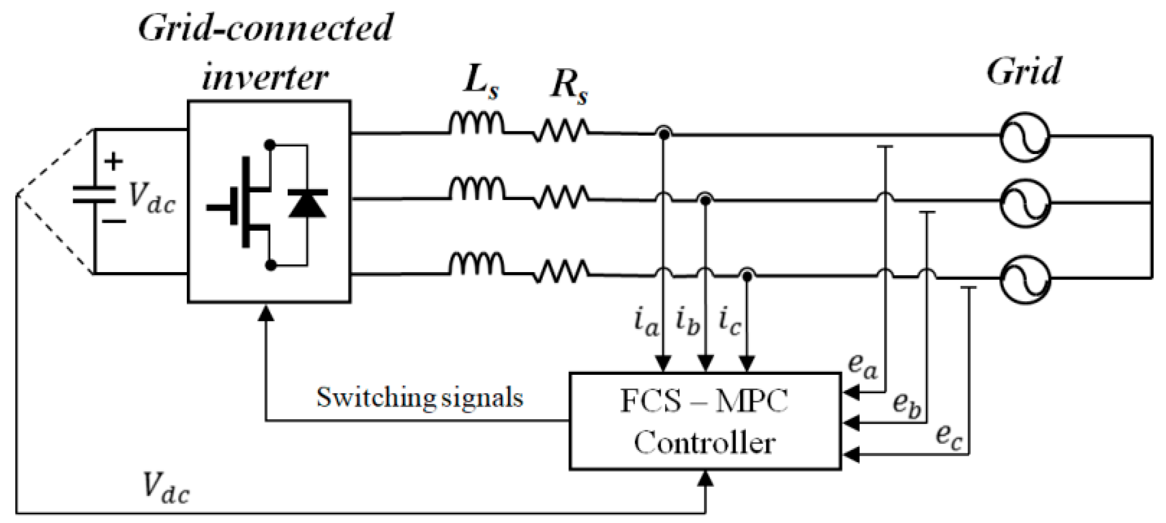
Finite control set–model predictive control (FCS-MPC) has been presented as a new approach to control the grid-connected inverter [16,17,18]. Contrary to the PI or the PR controllers, this control scheme directly drives the inverter switches without requiring the PWM technique. This method is proven to provide a very fast transient response. Moreover, it is possible to include more control objectives other than the current tracking due to the flexible nature of the cost function. However, this control scheme has a crucial disadvantage of variable switching frequency, which generates a wide spectrum of harmonic distortion even at low frequencies, leading to high total harmonic distortion (THD) value. In [19], a modulated MPC for a three-phase rectifier has been proposed to reduce the harmonic distortion in currents caused by the variable switching frequency. However, the distorted grid voltages have not been considered in this study. Moreover, this scheme is not effective to mitigate the harmonic currents in a grid-connected inverter in the presence of the distorted grid condition. Other methods considering multiple active voltage vectors during sampling time have been proposed in [20,21]. However, none of these methods have dealt with the presence of harmonic distortion in the grid voltages.

The main objective of this paper is to develop a current control scheme of improving the output currents in three-phase grid-connected inverter even when the grid voltages are severely distorted. The proposed scheme is based on the principle of the model predictive control, which determines the control signals by minimizing the cost function. Similar to the scheme in [19], the proposed scheme introduces weighting factors that are duty ratios of each individual active vector. Since each space vector is active for a certain duty interval during the sampling period, these duty ratios are chosen as the weighting factors for the corresponding vectors. This modification results in better THD performance in inverter output currents. While the existing scheme tries to reduce the harmonic distortion caused by the variable switching frequency in rectifier applications, the proposed scheme aims to mitigate the current harmonics of the grid-connected inverter under harmonic-distorted grid voltages. Furthermore, since the proposed scheme requires harmonic-free reference currents in the stationary reference frame to work successfully, the moving average filter (MAF) is used to enhance the performance of the phase lock loop (PLL) [22,23].As a result, the proposed control scheme can effectively control a grid-connected inverter with a good harmonic suppression capability during steady-state as well as transient periods even under adverse grid conditions. 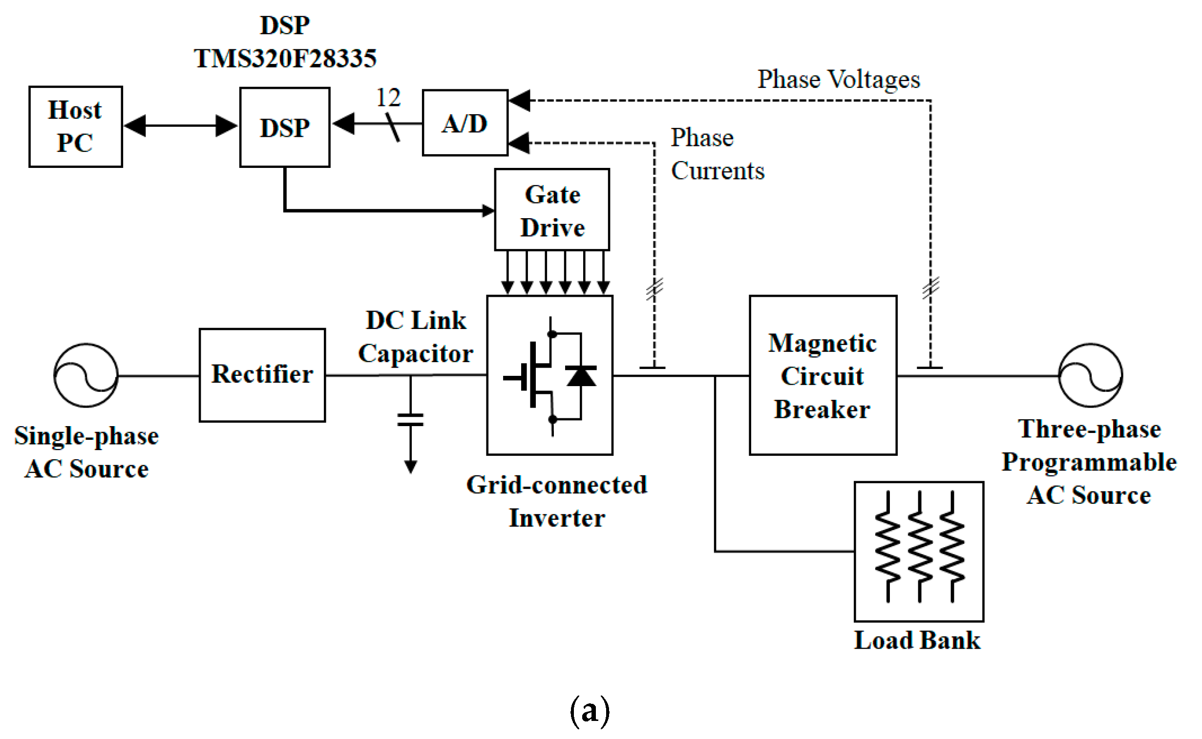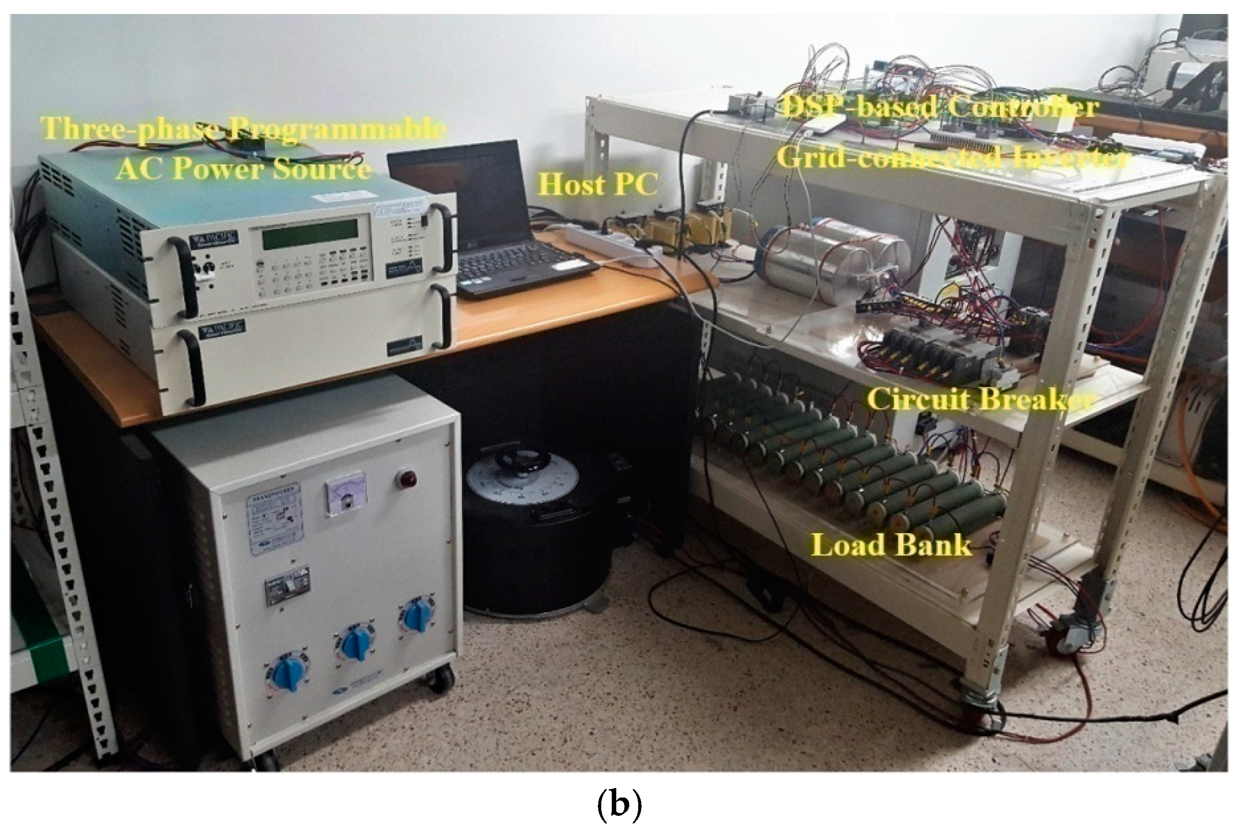The feasibility and effectiveness of the proposed scheme are verified through the comparative simulations and experiments using a prototype grid-connected inverter system based on digital signal processor (DSP) TMS320F28335 controller [24].

This paper is organized as follows: Section 2 presents a mathematical model of the system. Section 3 describes the proposed control scheme composed of the modulated FCS-MPC and MAF-PLL. Simulation results are presented in Section 4. Afterwards, the experimental results are given in Section 5. Finally, the conclusions are given in Section 6.

2. Modeling of a Grid-Connected Inverter

2.1. Modeling of a Grid-Connected Inverter with L-Filter

Since the MPC is a model-based controller as implied by the name, a precise system model and discretization are the key factors o design the controller successfully. To obtain the system model on the stationary reference frame, all three-phase variables are transformed into the variables on the stationary reference frame using the transformation matrix P as follows:

$${\left[e_{\alpha } e_{\beta }\right]}^T=P{\left[e_a e_{b } e_c\right]}^T$$

(1)

$${\left[v_{\alpha } v_{\beta }\right]}^T=P{\left[v_a v_b v_c\right]}^T$$

(2)

$${\left[i_{\alpha } i_{\beta }\right]}^T=P{\left[i_a i_b i_c\right]}^T,$$

(3)

where the subscript “αβ” denotes the variables on the stationary reference frame, the subscript “abc” denotes the variables in three-phase coordinate, $e_a$, $e_b$, and $e_c$ denote three-phase grid voltages, respectively, $v_a$, $v_b$, and $v_c$ are three-phase inverter output voltages, respectively, $i_a$, $i_b$, and $i_c$ represent three-phase inverter output currents, respectively, $e_{\alpha }$ and $e_{\beta }$ are the grid voltages in the stationary reference frame, respectively, $v_{\alpha }$ and $v_{\beta }$ represent the inverter output voltages in the stationary reference frame, respectively, $i_{\alpha }$ and $i_{\beta }$ are the inverter output currents in the stationary reference frame, and P is the transformation matrix expressed as:

$$P=\frac{2}{3}\left[\begin{array}{ccc}1& -\frac{1}{2}& -\frac{1}{2}\\ 0& -\frac{\sqrt{3}}{2}& \frac{\sqrt{3}}{2}\end{array}\right].$$

A three-phase grid-connected inverter is shown in Figure 1 in which $V_{dc}$ denotes the DC-link voltage. Considering the filter inductance $L_s$ and resistance $R_s$, the voltage equations of a grid-connected inverter in the stationary reference frame are presented as follows:

$$v_a=R_s{i}_a+L_s\frac{d{i}_a}{dt}+e_a$$

(4)

$$v_b=R_s{i}_b+L_s\frac{d{i}_b}{dt} +e_b$$

(5)

$$v_c=R_s{i}_c+L_s\frac{d{i}_c}{dt}+e_c.$$

(6)

Through the transformation, the voltage equations can be transformed into the stationary reference frame as follows:

$$v_{\alpha }=R_s{i}_{\alpha }+L_s\frac{d{i}_{\alpha }}{dt}+e_{\alpha }$$

(7)

$$v_{\beta }=R_s{i}_{\beta }+L_s\frac{d{i}_{\beta }}{dt}+e_{\beta }.$$

(8)

From Equations (7) and (8), a state-space model is derived as follows:

$$\frac{dx}{dt}=A\mathit{x}+B\mathit{u},$$

(9)

where $\mathit{x}={\left[i^T e^T\right]}^T={\left[i_{\alpha } i_{\beta } e_{\alpha } e_{\beta }\right]}^T$ is the state vector, $\mathit{u}={\left[v_{\alpha } v_{\beta }\right]}^T$ is the control vector, and the system matrices A and B are expressed as:

$$A=\left[\begin{array}{cccc}-\frac{R_s}{L_s}& 0& -\frac{1}{L_s}& 0\\ 0& -\frac{R_s}{L_s}& 0& -\frac{1}{L_s}\\ 0& 0& 0& -\omega \\ 0& 0& \omega & 0\end{array}\right],B=\left[\begin{array}{cc}\frac{1}{L_s}& 0\\ 0& \frac{1}{L_s}\\ 0& 0\\ 0& 0\end{array}\right].$$

The system states are controlled by the control vector u, which consists of the inverter output voltages in the stationary reference frame.

2.2. Discretization

The discrete-time model of the grid-connected inverter system at the time instant k can be expressed as:

$$\mathit{x}\left[k+1\right]=A_d\mathit{x}\left[k\right]+B_d\mathit{u}\left[k\right],$$

(10)

where A_d and B_d are the system and control matrices of the discrete-time state-space model and can be calculated as:

$$A_d=e^{A{T}_s}=I+\frac{A{T}_s}{1!}+\frac{A^2{T}_s^2}{2!}+\cdots =\left[\begin{array}{cccc}{a}_{11}& a_{12}& a_{13}& a_{14}\\ a_{21}& a_{22}& a_{23}& a_{24}\\ a_{31}& a_{32}& a_{33}& a_{34}\\ a_{41}& a_{42}& a_{43}& a_{44}\end{array}\right]$$

(11)

$$B_d=A^{-1}\left(A_d-I\right)B=\left[\begin{array}{cc}{b}_{11}& b_{12}\\ b_{21}& b_{22}\\ b_{31}& b_{32}\\ b_{41}& b_{42}\end{array}\right].$$

(12)

2.3. Output Voltage Vectors

With $2^3$ switching states, the switching vector s of a three-phase inverter is defined as follows:

$$s=\left[\begin{array}{c}{S}_a\\ S_b\\ S_c\end{array}\right], s\in S_{a, b,c}={\left\{1,-1\right\}}^3,$$

(13)

where S_a, S_b, and S_c denote the switching states for each phase. For the switching state $S_{a,b,c}=1$, the corresponding upper switch is turned on and the output terminal voltage becomes $+\frac{V_{dc}}{2}$. On the other hand, for the switching state $S_{a, b,c}=-1$, the corresponding lower switch is turned on and the output voltage of $-\frac{V_{dc}}{2}$ is applied.

The inverter output voltages in the stationary reference frame (αβ coordinate) can be obtained using the switching vector and transformation matrix as follows:

$${\left[v_{\alpha } v_{\beta }\right]}^T=P\times s\times \frac{V_{dc}}{2}.$$

(14)

The switching states and the corresponding output voltages in αβ coordinate are listed in

Table 1. Switching states and the corresponding output voltages in αβ coordinate.

Vector	${\mathit{S}}_{\mathit{a}}$	${\mathit{S}}_{\mathit{b}}$	${\mathit{S}}_{\mathit{c}}$	${\mathit{v}}_{\mathit{\alpha }}$	${\mathit{v}}_{\mathit{\beta }}$
0	−1	−1	−1	0	0
1	1	−1	−1	$\frac{2}{3}{V}_{dc}$	0
2	1	1	−1	$\frac{1}{3}{V}_{dc}$	$-\frac{\sqrt{3}}{3}{V}_{dc}$
3	−1	1	−1	$-\frac{1}{3}{V}_{dc}$	$-\frac{\sqrt{3}}{3}{V}_{dc}$
4	−1	1	1	$-\frac{1}{3}{V}_{dc}$	$\frac{\sqrt{3}}{3}{V}_{dc}$
5	−1	−1	1	$\frac{1}{3}{V}_{dc}$	$\frac{\sqrt{3}}{3}{V}_{dc}$
6	1	−1	1	$\frac{2}{3}{V}_{dc}$	0
7	1	1	1	0	0

.

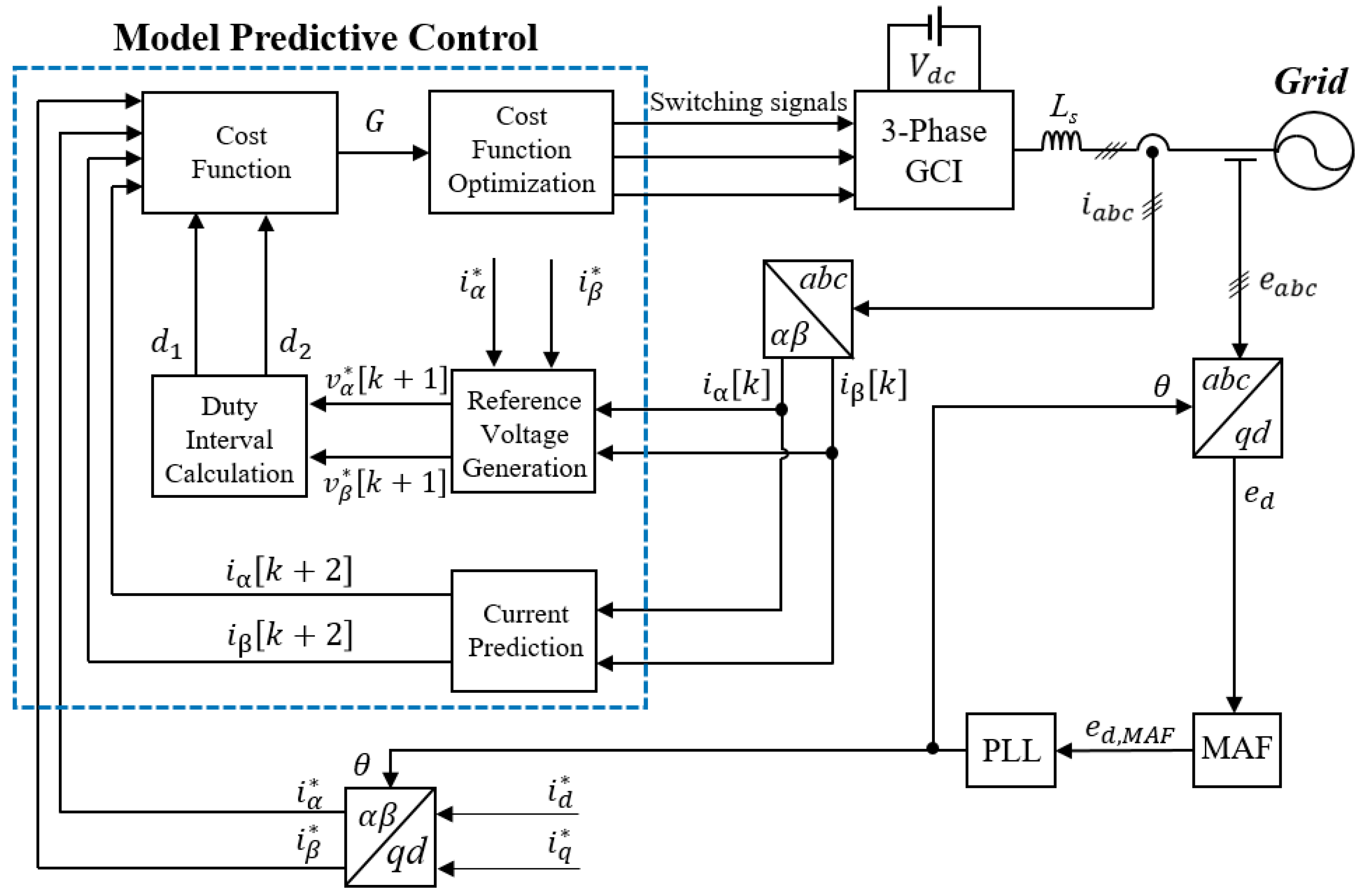
3. Proposed Control Scheme

A FCS-MPC scheme generally consists of the system model, cost function, and cost function optimization process. The system model is used to predict the system behavior in the future. The cost function is obtained based on the control objectives of system, which are usually the error between the predicted current and reference value. This cost function is minimized during the optimization process. Once the cost function is minimized, the control signals that minimize the cost function are fed into the inverter. In the traditional FCS-MPC method, the determined switching states of inverter are applied during the whole sampling period, which increases the current harmonics in wide spectrum. Since these harmonics are very difficult to filter out, it causes the decrease in the quality of output current.

Figure 2 shows the block diagram of the proposed FCS-MPC scheme for a grid-connected inverter, in which the inverter is connected to the grid through L filter. In the proposed method, the duty intervals d₁ and d₂ for each active voltage vector are calculated based on the reference voltages. These duty intervals, the predicted currents, and the harmonic-free reference currents generated by the MAF-PLL are used to obtain the cost function. The cost function is optimized to produce the switching signals for the grid-connected inverter.

3.1. Prediction of Output Currents

Assuming that the system variables are constant during each sampling interval, the prediction of currents can be obtained from the discrete-time model in Equation (10) as follows:

$$i_{\alpha }\left[k+1\right]=a_{11}\times i_{\alpha }\left[k\right]+a_{13}\times e_{\alpha }\left[k\right]+a_{14}\times e_{\beta }\left[k\right]+b_{11}\times v_{\alpha }\left[k\right]$$

(15)

$$i_{\beta }\left[k+1\right]=a_{22}\times i_{\beta }\left[k\right]+ a_{23}\times e_{\alpha }\left[k\right]+a_{24}\times e_{\beta }\left[k\right]+b_{22}\times v_{\beta }\left[k\right].$$

(16)

In a digital implementation of the control algorithm, the control signals cannot be applied instantly to inverter. Instead, the control signals determined at the present step are only applicable at the next sampling period, which results in a time delay. In order to consider and compensate this time delay, two-step-ahead prediction of currents is introduced in the control algorithm as follows:

$$i_{\alpha }\left[k+2\right]=\left(a_{11}\times i_{\alpha }\left[k+1\right]+a_{13}\times e_{\alpha }\left[k+1\right] + a_{14}\times e_{\beta }\left[k+1\right]\right)+b_{11}\times v_{\alpha }\left[k+1\right]$$

(17)

$$i_{\beta }\left[k+2\right]=(a_{22}\times i_{\beta }\left[k+1\right]+a_{23}\times e_{\alpha }\left[k+1\right]+a_{24}\times e_{\beta }\left[k+1\right])+b_{22}\times v_{\beta }\left[k+1\right].$$

(18)

When the zero vector 0 or 7 in Table 1 is applied, the predicted currents at the sampling instant (k+2) can be obtained as follows:

$$i_{\alpha }^0\left[k+2\right]=a_{11}\times i_{\alpha }\left[k+1\right]+a_{13}\times e_{\alpha }\left[k+1\right] + a_{14}\times e_{\beta }\left[k+1\right]$$

(19)

$$i_{\beta }^0\left[k+2\right]=a_{22}\times i_{\beta }\left[k+1\right]+a_{23}\times e_{\alpha }\left[k+1\right]+a_{24}\times e_{\beta }\left[k+1\right],$$

(20)

where $i_{\alpha }^0$ and $i_{\beta }^0$ denote the predicted output currents in αβ coordinate when the zero vector is applied.

Substituting Equations (19) and (20) into Equations (17) and (18) results in:

$$i_{\alpha }\left[k+2\right]=i_{\alpha }^0\left[k+2\right]+b_{11}\times v_{\alpha }\left[k+1\right]$$

(21)

$$i_{\beta }\left[k+2\right]=i_{\beta }^0\left[k+2\right]+b_{22}\times v_{\beta }\left[k+1\right].$$

(22)

According to Table 1, a three-phase inverter has eight possible output voltage vectors. Unlike the conventional FCS-MPC scheme that applies the switching states during the whole sampling period, the proposed control strategy mimics the behavior of the PWM by applying three vectors during each sampling period. Two active voltage vectors are applied for the duty intervals of d₁ and d₂ while the zero vector is applied for the remaining time of the sampling period. In this case, the average voltages produced by inverter can be calculated as:

$$V_{\alpha }\left[k+1\right]=\left[d_1{v}_{\alpha }^i+d_2{v}_{\alpha }^j\right]$$

(23)

$$V_{\beta }\left[k+1\right]=\left[d_1{v}_{\beta }^i+d_2{v}_{\beta }^j\right],$$

(24)

where $v_{\alpha }^i$ and $v_{\beta }^i$ denote the output voltages in αβ coordinate according to the voltage vector i, and $\left(i,j\right)$ represents a pair of the adjacent active vectors among six possible pairs as follows:

$$\left(i,j\right)=\left(1,2\right),\left(2,3\right),\left(3,4\right),\left(4,5\right),\left(5,6\right),\left(6,1\right).$$

(25)

The prediction of output currents can be calculated from Equations (21) and (22) for each pair of the active vectors $\left(i,j\right)$ as follows:

$$i_{\alpha }^i\left[k+2\right]=i_{\alpha }^0\left[k+2\right]+b_{11}\times v_{\alpha }^i\left[k+1\right]$$

(26)

$$i_{\beta }^i\left[k+2\right]=i_{\beta }^0\left[k+2\right]+b_{22}\times v_{\beta }^i\left[k+1\right]$$

(27)

$$i_{\alpha }^j\left[k+2\right]=i_{\alpha }^0\left[k+2\right]+b_{11}\times v_{\alpha }^j\left[k+1\right]$$

(28)

$$i_{\beta }^j\left[k+2\right]=i_{\beta }^0\left[k+2\right]+b_{22}\times v_{\beta }^j\left[k+1\right],$$

(29)

where $i_{\alpha }^i$ and $i_{\beta }^i$ denote the inverter output currents in αβ coordinate corresponding to the voltage vector i.

3.2. Generation of Reference Voltages

The current errors between the reference and predicted values are defined as follows:

$$\Delta i_{\alpha }\left(k+2\right)=i_{\alpha }^{*}\left[k+2\right]-i_{\alpha }\left[k+2\right]$$

(30)

$$\Delta i_{\beta }\left(k+2\right)=i_{\beta }^{*}\left[k+2\right]-i_{\beta }\left[k+2\right],$$

(31)

where the symbol “*” denotes the reference quantity. In order to achieve the control objective that reduces the tracking error to zero, it is reasonable to assume:

$$i_{\alpha }^{*}\left[k+2\right]=i_{\alpha }\left[k+2\right]$$

(32)

$$i_{\beta }^{*}\left[k+2\right]=i_{\beta }\left[k+2\right].$$

(33)

Substituting Equations (32) and (33) into Equations (21) and (22) results in:

$$i_{\alpha }^{*}\left[k+2\right]=i_{\alpha }^0\left[k+2\right]+b_{11}\times v_{\alpha }\left[k+1\right]$$

(34)

$$i_{\beta }^{*}\left[k+2\right]=i_{\beta }^0\left[k+2\right]+b_{22}\times v_{\beta }\left[k+1\right].$$

(35)

From Equations (34) and (35), the desired expressions for the output voltage references that achieve zero tracking error can be obtained as:

$$v_{\alpha }^{*}\left[k+1\right]=\frac{i_{\alpha }^{*}\left[k+2\right]-i_{\alpha }^0\left[k+2\right]}{b_{11}}$$

(36)

$$v_{\beta }^{*}\left[k+1\right]=\frac{i_{\beta }^{*}\left[k+2\right]-i_{\beta }^0\left[k+2\right]}{b_{22}}.$$

(37)

3.3. Calculation of Duty Intervals

Using Equations (23) and (24), the output voltage references can be expressed in terms of the output voltage vectors and duty intervals as:

$$v_{\alpha }^{*}\left[k+1\right]=\left[d_1{v}_{\alpha }^i+d_2{v}_{\alpha }^j\right]$$

(38)

$$v_{\beta }^{*}\left[k+1\right]=\left[d_1{v}_{\beta }^i+d_2{v}_{\beta }^j\right].$$

(39)

From Equations (38) and (39), the duty intervals of each active voltage vector are obtained as follows:

$$d_1=\frac{v_{\beta }^{*}\left[k+1\right]v_{\alpha }^j-v_{\alpha }^{*}\left[k+1\right]v_{\beta }^j}{v_{\alpha }^j{v}_{\beta }^i-v_{\alpha }^i{v}_{\beta }^j}$$

(40)

$$d_2=\frac{v_{\beta }^{*}\left[k+1\right]v_{\alpha }^i-v_{\alpha }^{*}\left[k+1\right]v_{\beta }^i}{v_{\alpha }^i{v}_{\beta }^j-v_{\alpha }^j{v}_{\beta }^i} .$$

(41)

The zero vector is applied for the remaining time of the sampling period as:

$$d_o=1-d_1-d_2,$$

(42)

where d_o denotes the duty interval of the zero vector. These duty intervals are calculated for each pair of the active voltage vectors $\left(i,j\right)$ in Equation (25) similar to the prediction algorithm of output currents.

3.4. Cost Function Minimization

Both the prediction of output currents and the calculation of duty intervals are processed simultaneously for each pair of the active voltage vectors defined in Equation (25). Based on these values, the cost functions for each pair of the active voltage vectors are calculated as follows:

$$G^i=\sqrt{{\left(i_{\alpha }^{*}\left[k+2\right]-i_{\alpha }^i\left[k+2\right]\right)}^2+{\left(i_{\beta }^{*}\left[k+2\right]-i_{\beta }^i\left[k+2\right]\right)}^2}$$

(43)

$$G^j=\sqrt{{\left(i_{\alpha }^{*}\left[k+2\right]-i_{\alpha }^j\left[k+2\right]\right)}^2+{\left(i_{\beta }^{*}\left[k+2\right]-i_{\beta }^j\left[k+2\right]\right)}^2}$$

(44)

$$G=d_1{G}^i+d_2{G}^j.$$

(45)

Since each vector is applied for duty intervals $d_1$ and $d_2$, respectively, these duty intervals are used as the weighting factors to evaluate the effect of each vector in the final cost function in Equation (45). In every sampling period, the cost functions $G$ are calculated for six possible pairs of voltage vectors in Equation (25). These values of the cost function calculated for six possible pairs are compared with each other to determine the minimum value of the cost function. Then, the pair of active vectors that produces the minimum value of the cost function $G$ is chosen to apply these active vectors to inverter in the next sampling period.

3.5. Harmonic Mitigation and MAF-PLL

The purpose of the proposed scheme is to minimize the error between the reference currents and predicted ones by using the cost functions in Equations (43)–(45). Since the proposed scheme is designed in the stationary reference frame, the stationary reference currents without harmonic distortion are required for the proposed scheme to work successfully with the high quality of inverter output currents. The PLL scheme is generally employed in a grid-connected inverter in order to achieve the synchronization of DG system with the main grid. For this purpose, the traditional synchronous reference frame phase lock loop (SRF-PLL) has been usually employed in applications of the grid-connected inverter to determine the angular displacement of grid voltage. However, due to the limitation of the PI controller, the performance of this scheme deteriorates significantly when it operates under distorted grid condition. In this condition, the resulting grid angular displacement often contains the harmonic contents caused by the distorted grid voltages. If the reference currents in αβ coordinate are generated by using this angular displacement contaminated by harmonic distortion, the reference currents are also distorted with the harmonic contents, resulting in the performance degradation of the proposed control scheme.

To obtain pure sinusoidal reference currents in αβ coordinate, the MAF-PLL is used to replace the traditional SRF-PLL in the proposed scheme. The MAF-PLL scheme employs the MAF as an ideal low pass filter to obtain the DC-quantity of the d-axis voltage [13].The transfer function of the MAF can be described as:

$$H_{MAF}\left(\mathrm{s}\right)\approx \frac{1}{\frac{T_w}{2}s+1},$$

(46)

where T_w is the window length of the MAF. The transfer function of the MAF-PLL can be obtained from Equation (46) and the conventional SRF-PLL as follows:

$$H_{MAF-PLL}\left(\mathrm{s}\right)=H_{MAF}\left(\mathrm{s}\right)\times \frac{k_{p}s+k_{i}s}{s^2},$$

(47)

where $k_p$ and $k_i$ denote the PI gains of the SRF-PLL, respectively. The MAF-PLL method is capable of detecting the grid phase angle accurately even when the grid voltages are highly distorted. From this phase angle information, the stationary sinusoidal reference currents can also be generated without harmonic contamination.

Sinusoidal reference currents can be also obtained from the BPF-based harmonic extraction, as in [12]. However, the use of the BPF results in much slower transient response in comparison to that of the MAF-PLL due to the sluggish dynamics of the BPF. The simulation results are given to demonstrate the effect of the MAF-PLL on current control performance.

4. Simulation Results

In order to prove the feasibility of the proposed FCS-MPC with modulation for a grid-connected inverter as depicted in Figure 2, the simulations have been done. The system parameters are summarized in

Table 2. System parameters of a grid-connected inverter.

Parameters	Symbol	Value	Units
Rated power	PR	2	kW
Grid voltage	E	180	V
Grid frequency	F	60	Hz
DC-link voltage	Vdc	420	V
Filter inductance	Ls	7	mH
Filter resistance	Rs	0.5	Ω
Switching frequency	fs	10	kHz

.

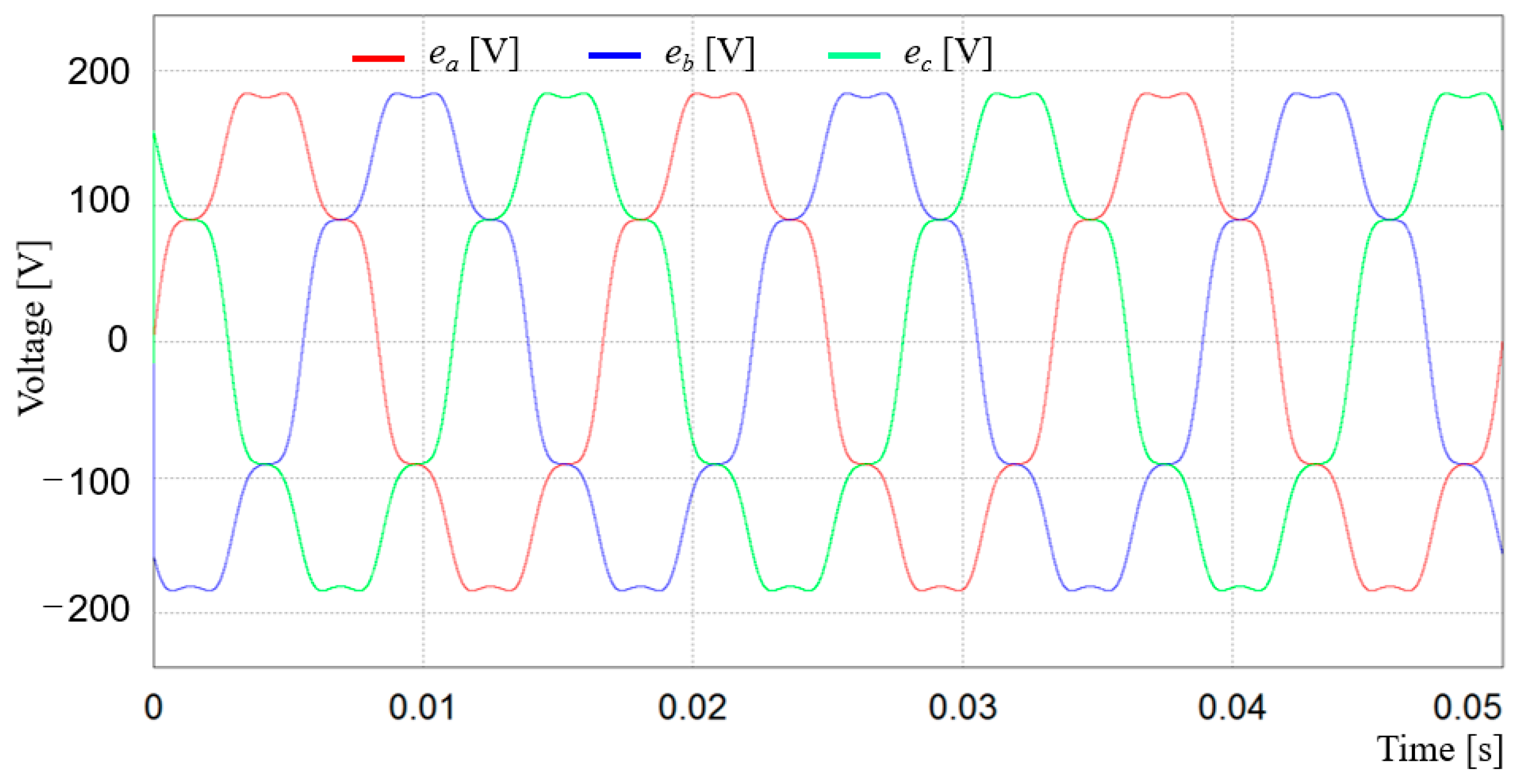
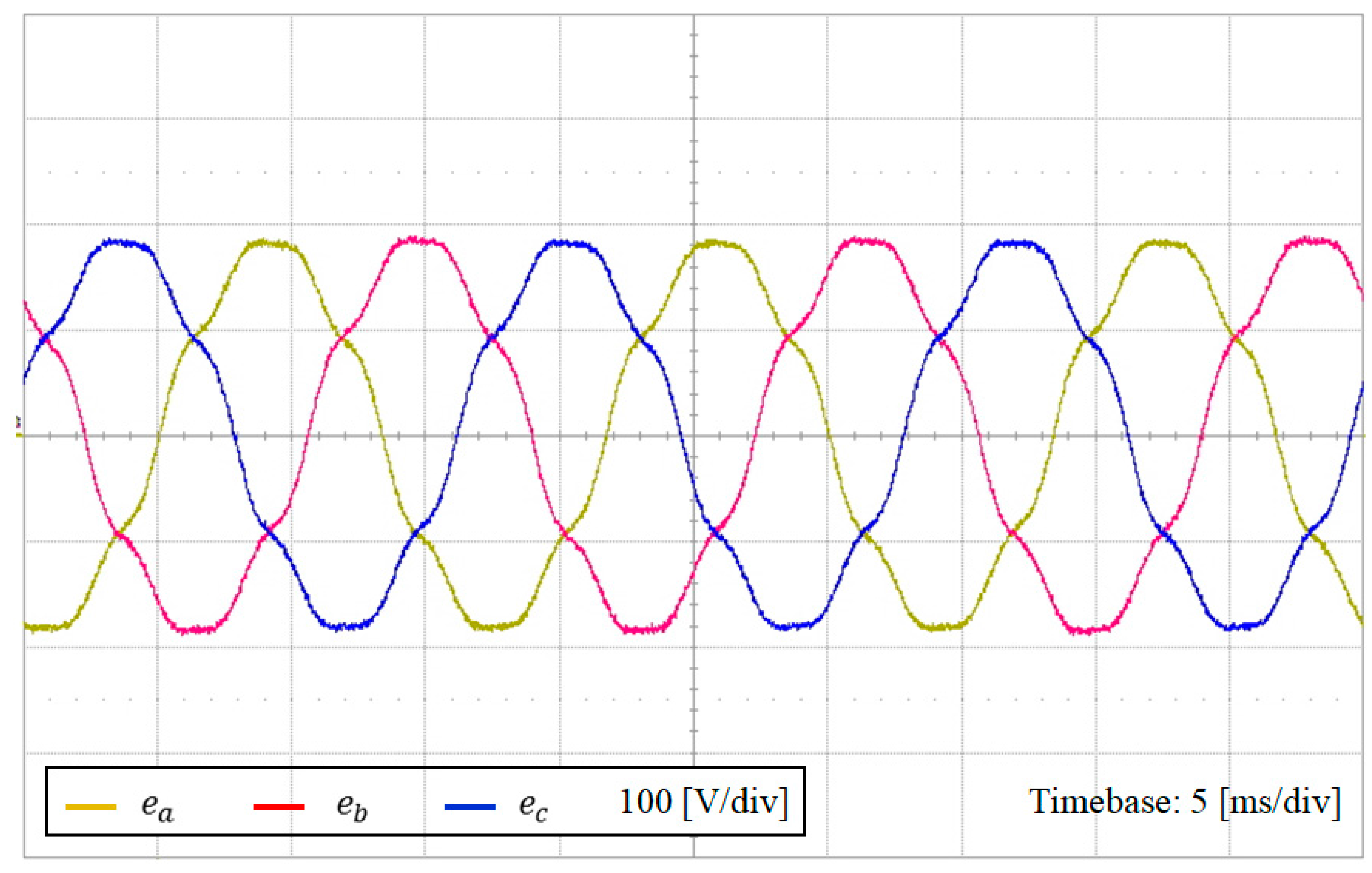
The harmonic compensation capability of the proposed control scheme is evaluated using the PSIM software under a distorted grid condition. For an adverse grid condition, the 5th and 7th harmonics with 10% of the fundamental component and the 11th and 13th harmonics with 1% of the fundamental component are injected to the ideal grid voltages. The resultant waveform of the distorted grid voltages is demonstrated in Figure 3.

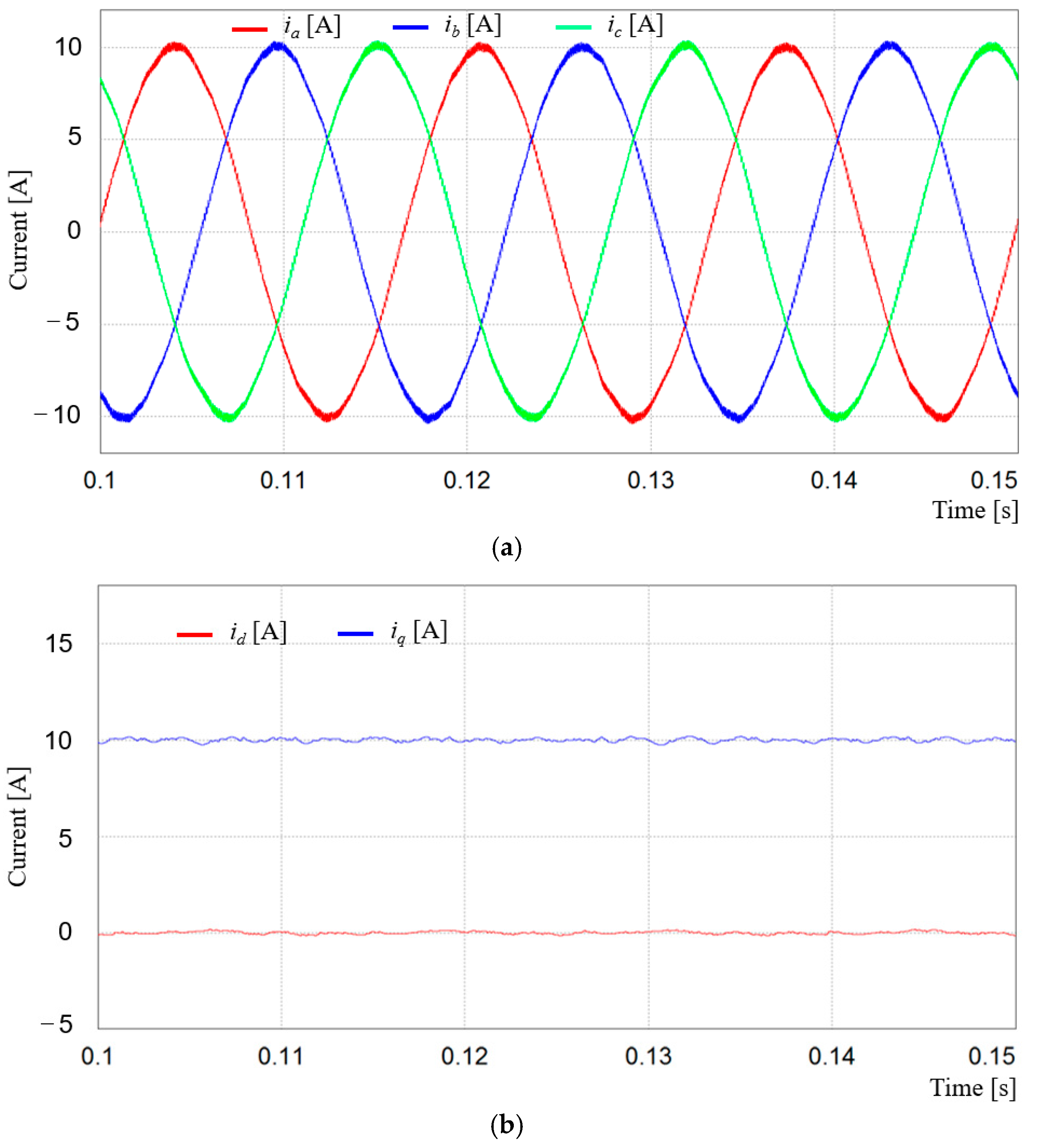
Figure 4 shows the performance of the conventional PI decoupling controller under the ideal grid condition for comparison purpose. It can be clearly seen that the PI decoupling controller performs well under such a condition and does not give a severe harmonic distortion in three-phase output currents. As is shown in Figure 4b, the q-axis and d-axis currents i_q and i_d are well controlled to track the reference currents without steady-state errors or fluctuation.

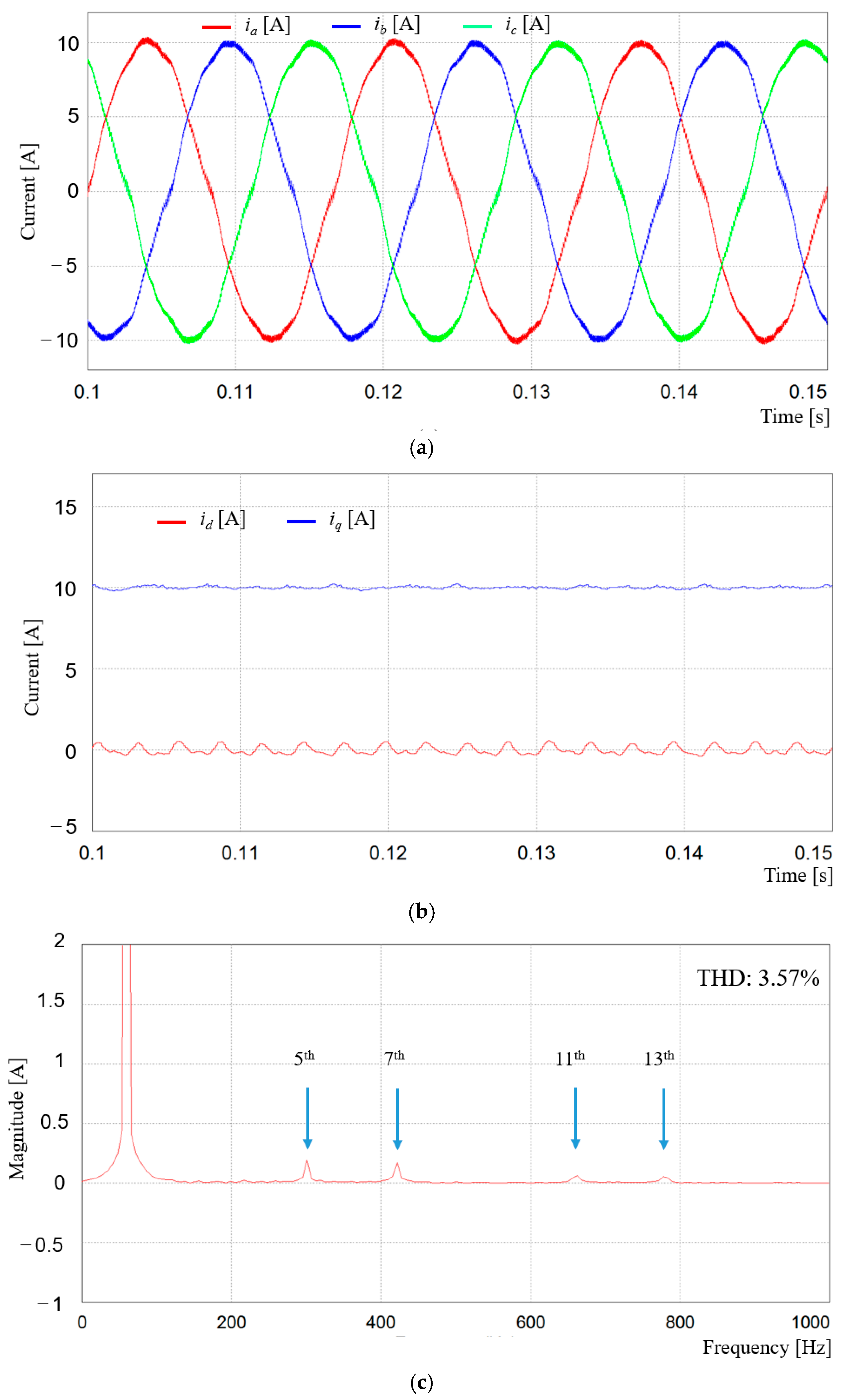
Figure 5 shows the performance of the same PI controller under distorted grid voltages as shown in Figure 3. As is obviously shown in Figure 5a, the performance of this controller is not satisfactory any longer, developing considerable harmonic contents in three-phase current waveforms due to the distorted grid voltages. In addition, the q-axis and d-axis currents i_q and i_d show large fluctuation caused by the harmonic components. This performance deterioration comes from the traditional SRF-PLL and the existence of the grid disturbance due to harmonic distortion. The SRF-PLL scheme cannot completely filter out the effect of harmonic contents in grid voltages in obtaining the angular displacement and angular frequency. Moreover, the PI controller naturally has a poor disturbance rejection capability. The FFT result of phase current in Figure 5c shows that there exist the 5th, 7th, 11th, and 13th harmonics in the output currents, which leads to a relatively high THD value of 3.57%.

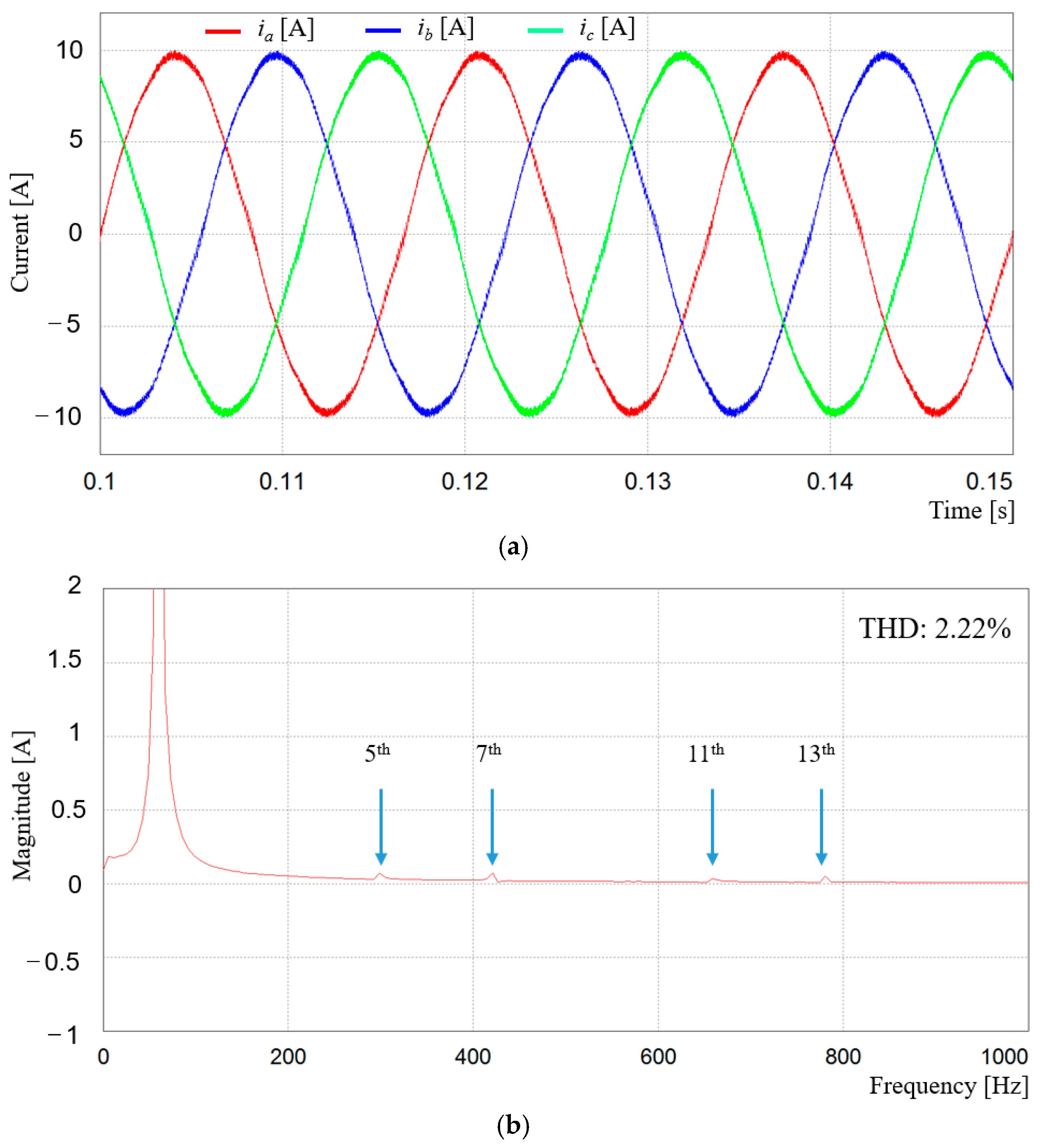
The PR controller is another classical control method that is usually employed in a grid-connected inverter application with the purpose of reducing the harmonics in inverter output currents. In Figure 6, the performance of the PR controller is presented under the same distorted grid voltages shown in Figure 3. Despite of giving more sinusoidal phase currents as compared with the case of the PI controller, a slight distortion in phase current is still observed. This distortion can be seen more clearly in the FFT result of a-phase current in Figure 6b, which shows small 5th, 7th, 11th, and 13th harmonic components. The resultant THD value is 2.22%, which is lower than the case of the PI controller.

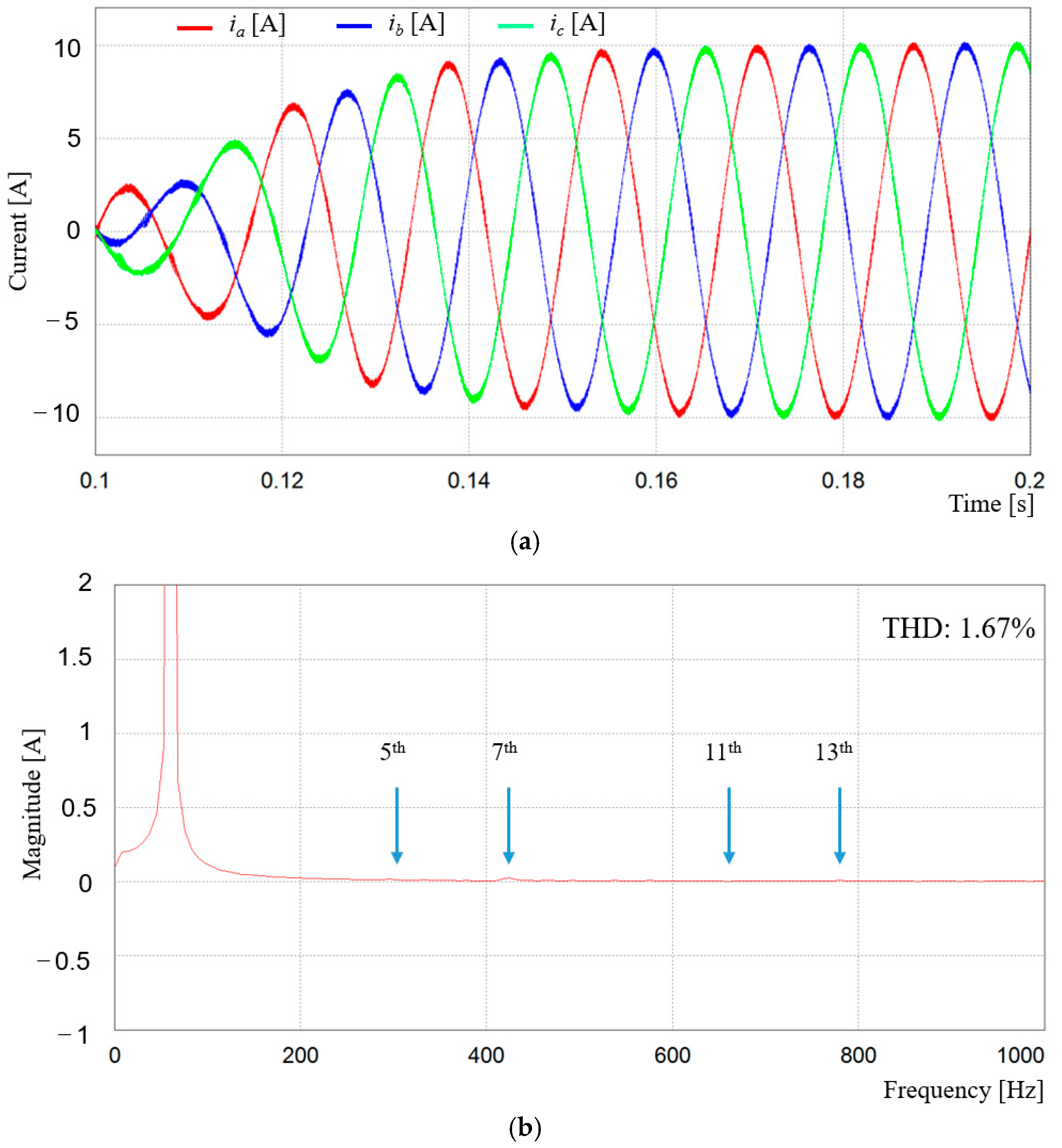
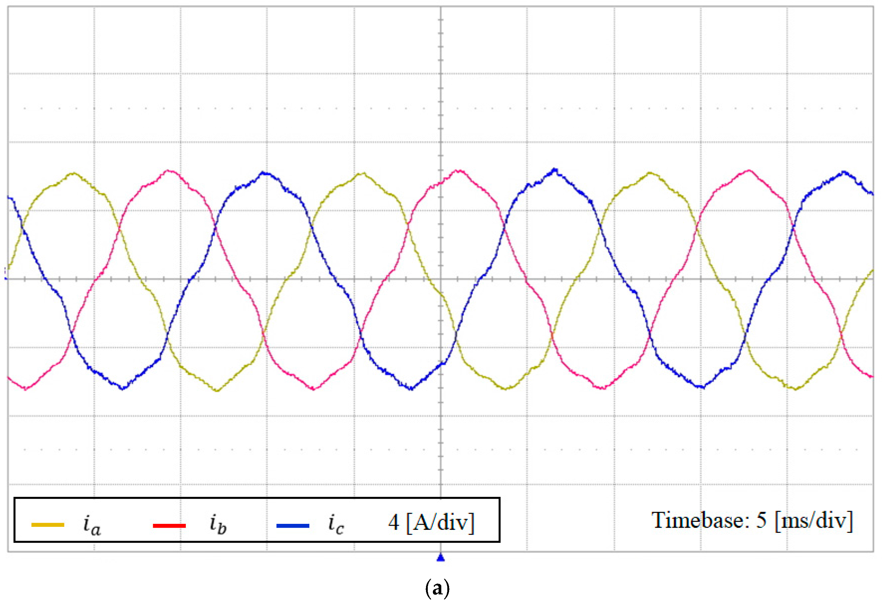
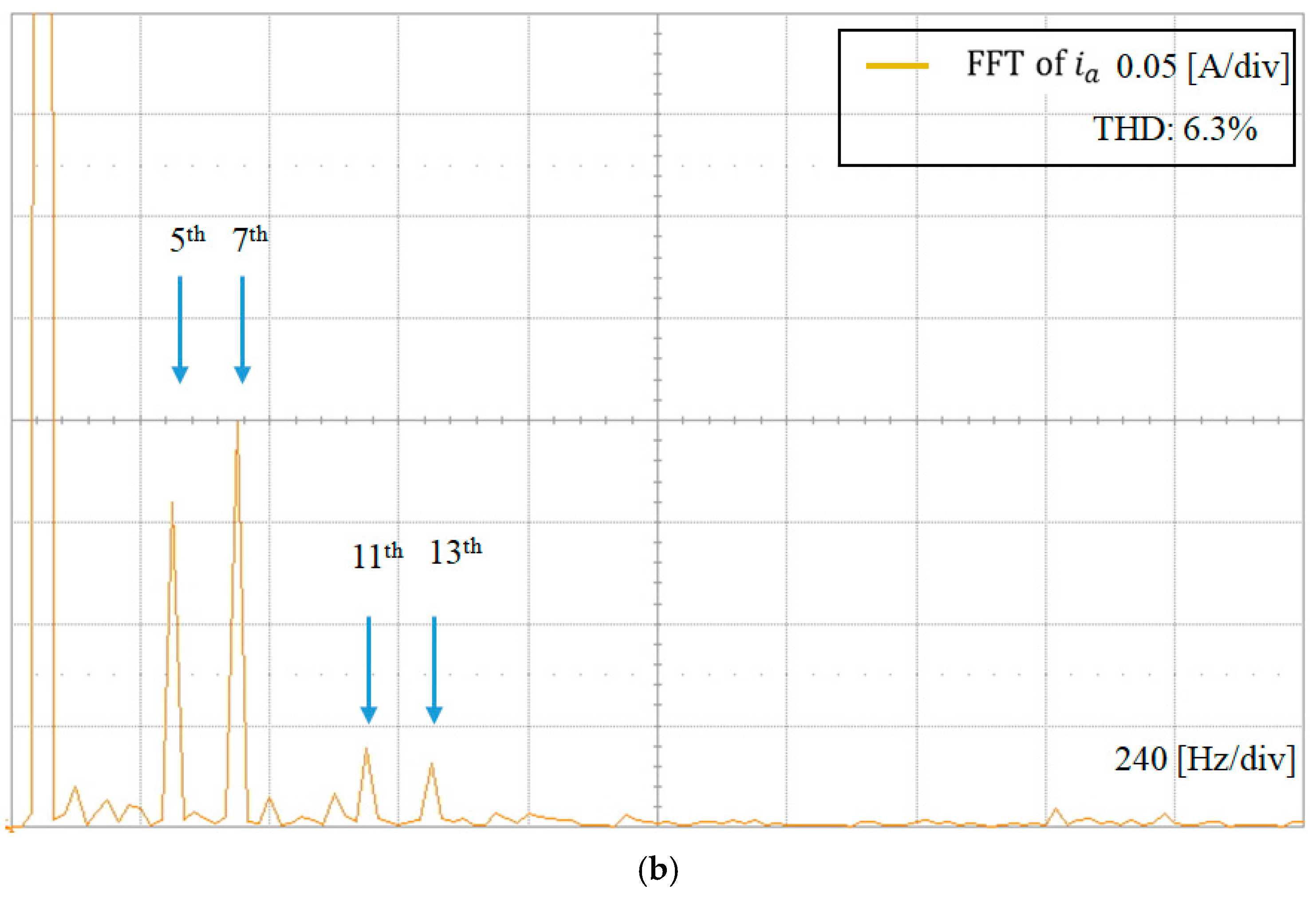
In comparison with conventional PI and PR controllers, the performance of the proposed FCS-MPC scheme with modulation under the same distorted grid condition is shown in Figure 7, in which the BPF is employed in the SRF-PLL to obtain the grid angular displacement without the influence of the harmonic-distorted grid voltages, and thus, to generate pure sinusoidal reference currents in αβ coordinate without the harmonic contamination. Due to an effective harmonic suppression, the phase current waveforms remain quite sinusoidal in spite of an abnormal grid condition as shown in Figure 7a in contrast with those in Figure 5 and Figure 6. In addition, the FFT result of phase current in Figure 7b shows only a negligible amount of harmonic contents. The THD value is 1.67%, which is smaller than both the PI controller and the PR controller, being comparable to the THD value of the PI controller under the ideal grid condition. Although the harmonic mitigation in inverter currents can be achieved at steady state even under the distorted grid voltages by using the proposed FCS-MPC scheme with modulation and the BPF, the transient response becomes slower than that of the conventional control schemes, which is not acceptable for DG applications since the current dynamics are supposed to be faster than those of outer-loop system. Such a slow transient results from the adoption of the BPF in the SRF-PLL to obtain the harmonic-free reference currents in the stationary frame. The BPF normally takes a considerable time for the filter output to reach the steady state.

In order to improve the transient response while retaining a good harmonic mitigation performance, the PLL scheme based on the MAF is introduced instead of the BPF. The MAF is able to filter out the harmonic contents in grid voltages faster than the BPF. Thus, the purpose of the MAF-PLL is to obtain the angular displacement and angular frequency rapidly without harmonic distortion. In view of the computational burden as well as the dynamic response, the MAF has been regarded as a more effective way as compared with the BPF [13]. Through the MAF-PLL, the harmonic-free sinusoidal reference currents on the stationary reference frame can be generated more simply and rapidly than the BPF case. These sinusoidal reference currents play an important role in improving the quality of inverter output currents.

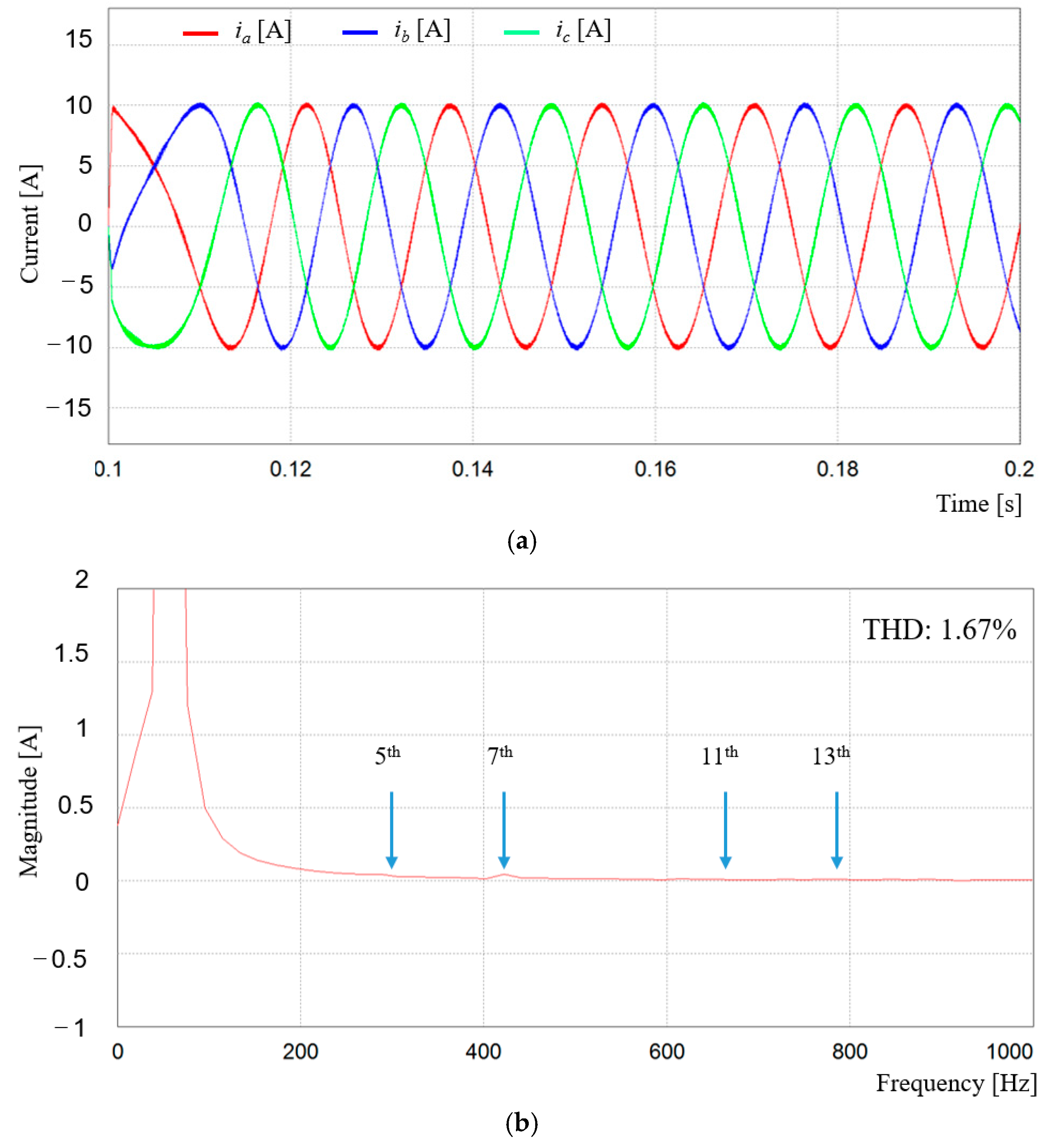
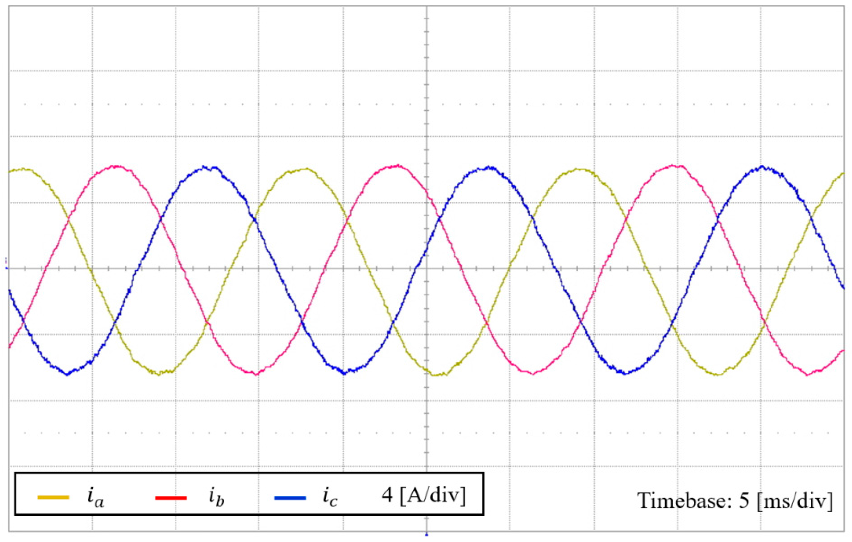
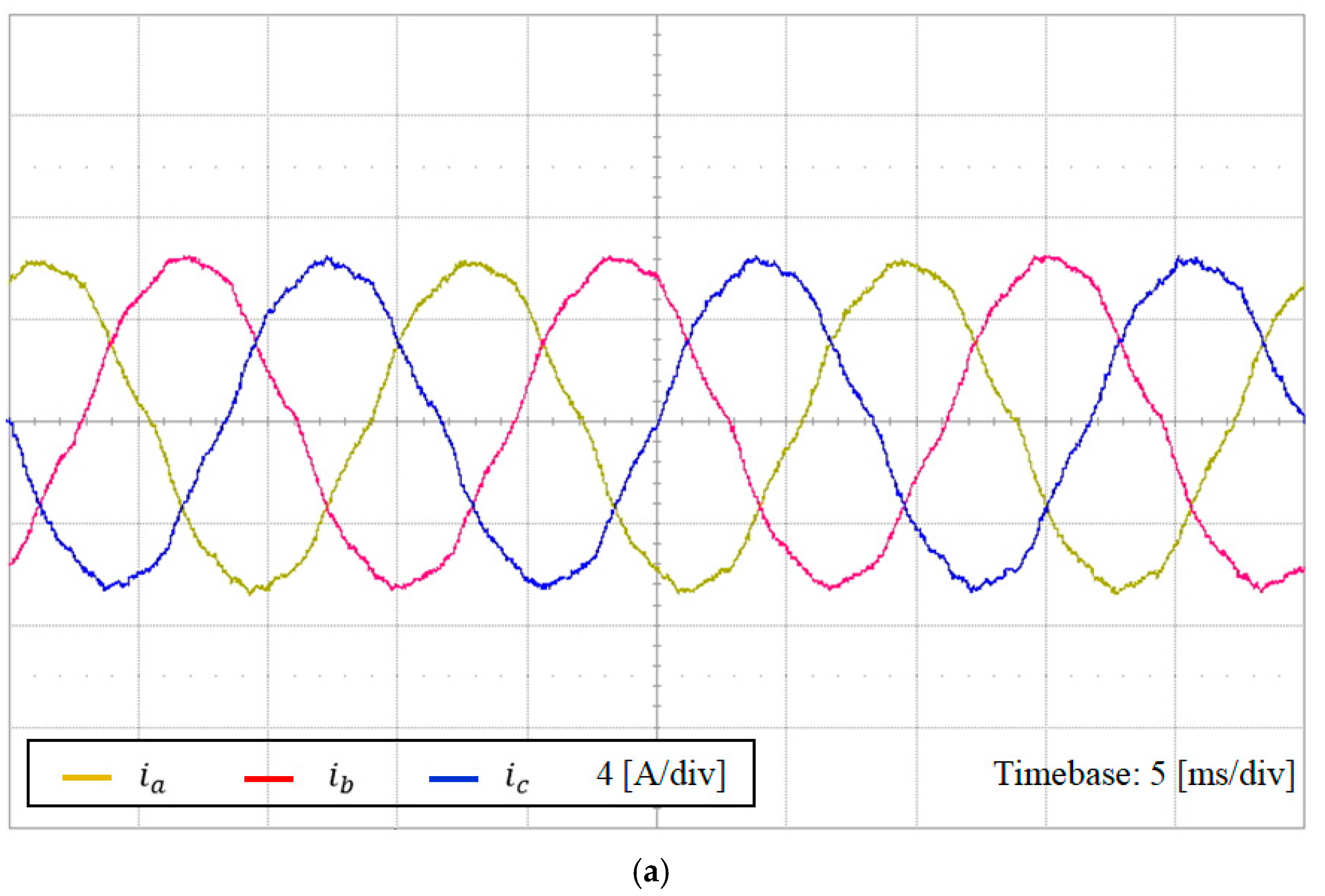
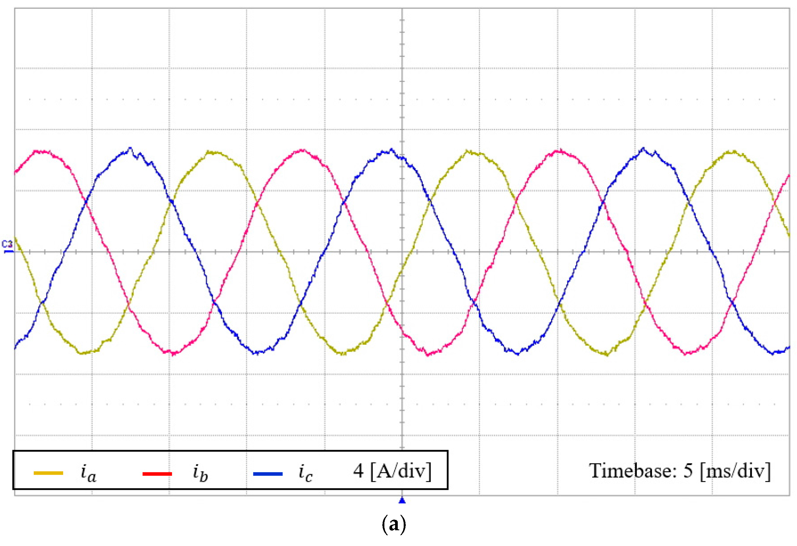
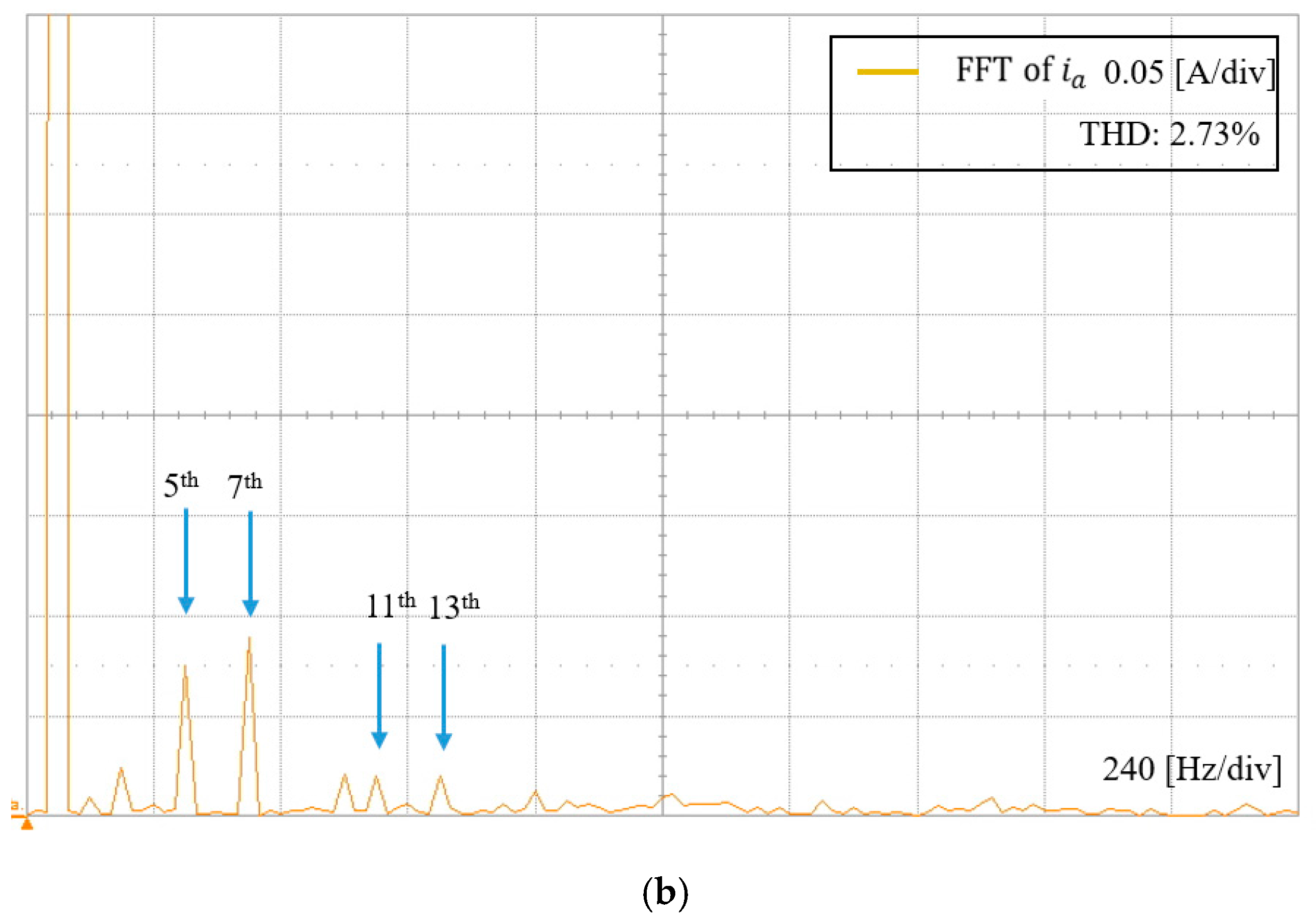
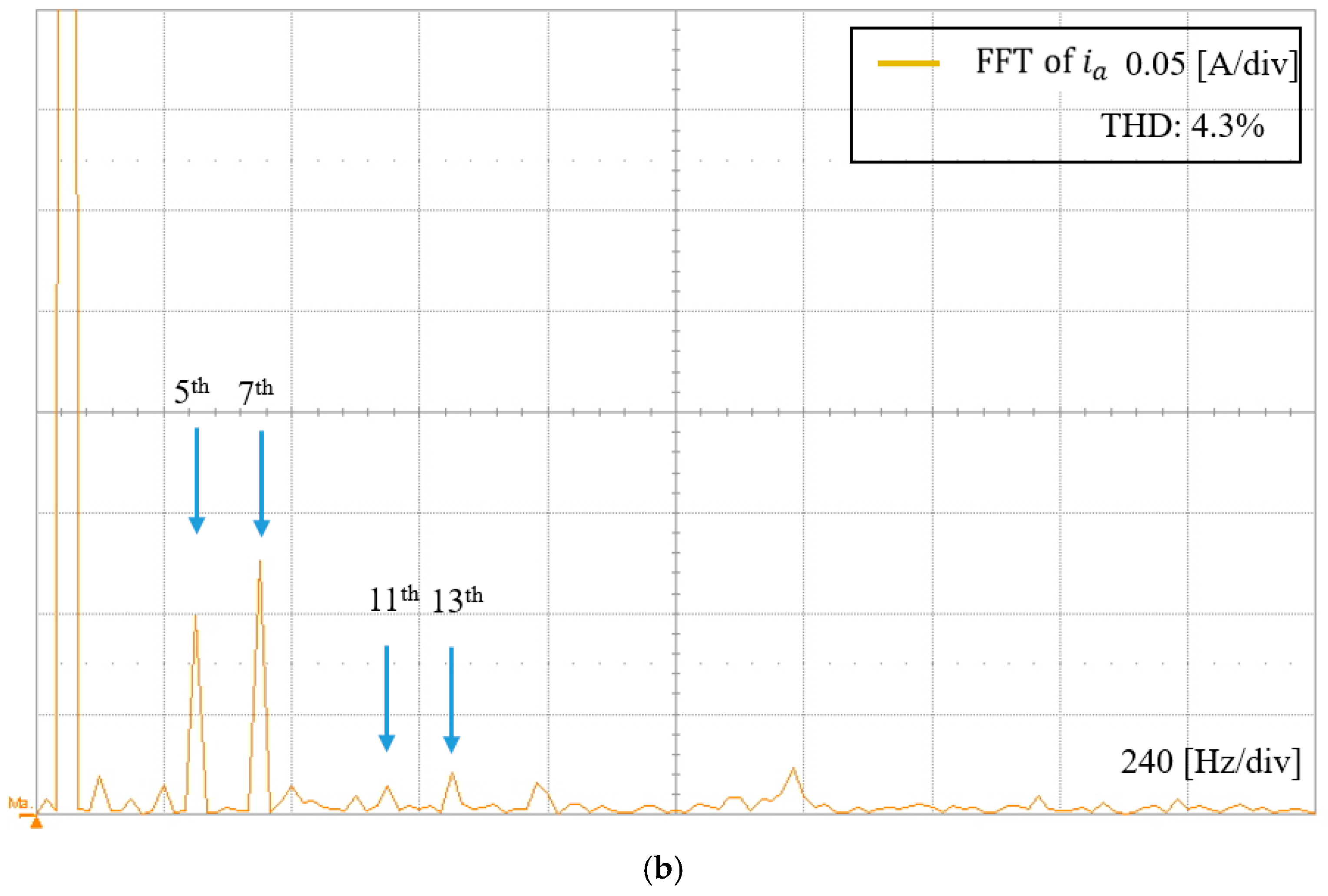
Figure 8 shows the proposed control scheme consisting of the modulated FCS-MPC and MAF-PLL under the same distorted grid condition. The phase current waveforms in Figure 8a are similarly sinusoidal at steady state as in Figure 7a. Also, the FFT result of a-phase current shown in Figure 8b is consistent with the case in Figure 7b, showing only negligible harmonics with the THD value of 1.67%. This FFT result satisfies the harmonic current regulation limit stated in IEEE std. 1547. In addition to an improved harmonic suppression at steady state, the proposed scheme shows much faster transient response than Figure 7. In Figure 8a, the transient lasts only half a cycle before reaching steady state.

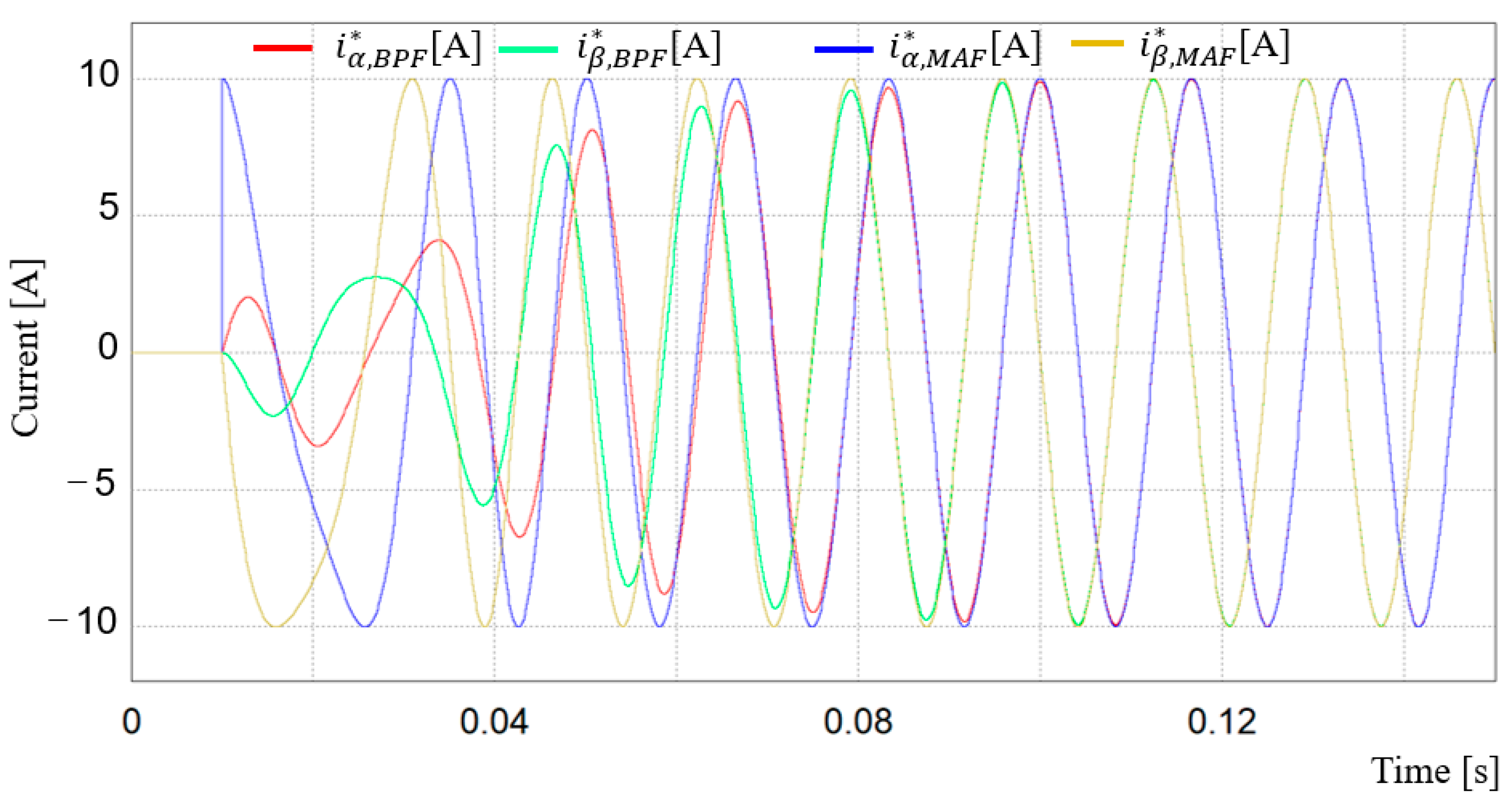
Figure 9 shows the comparison of the generation of the reference currents in αβ coordinate between the BPF and MAF. While both schemes generate pure sinusoidal reference currents at steady state, the transient response of the MAF is much smaller than that of the BPF.

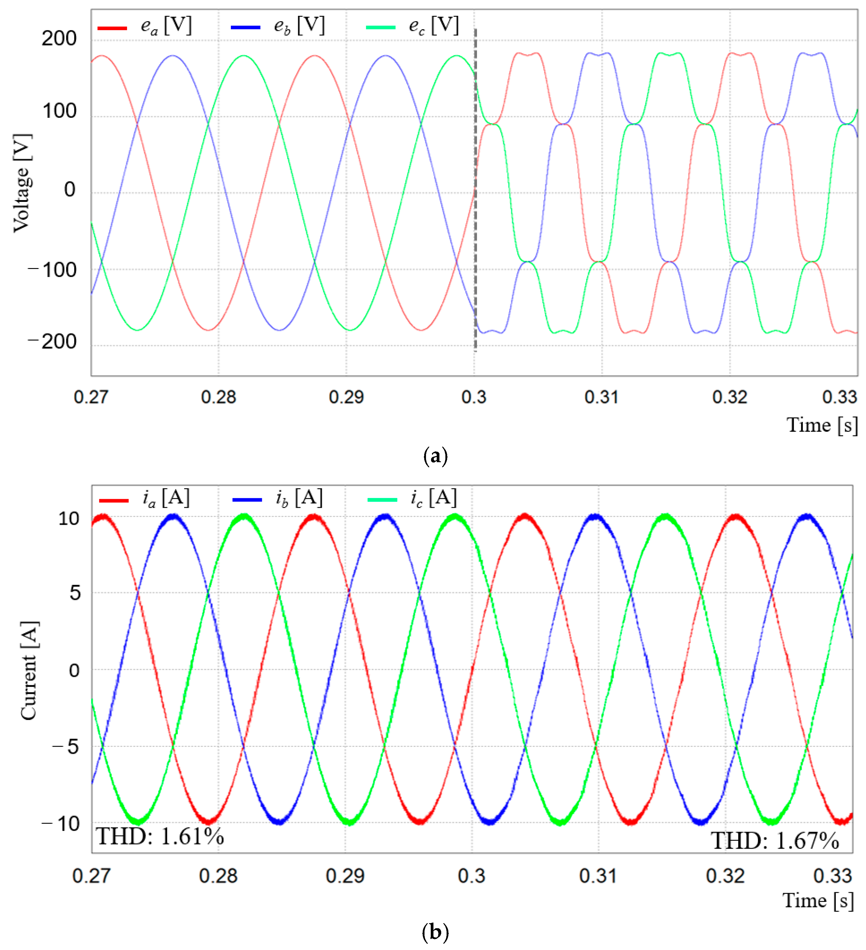
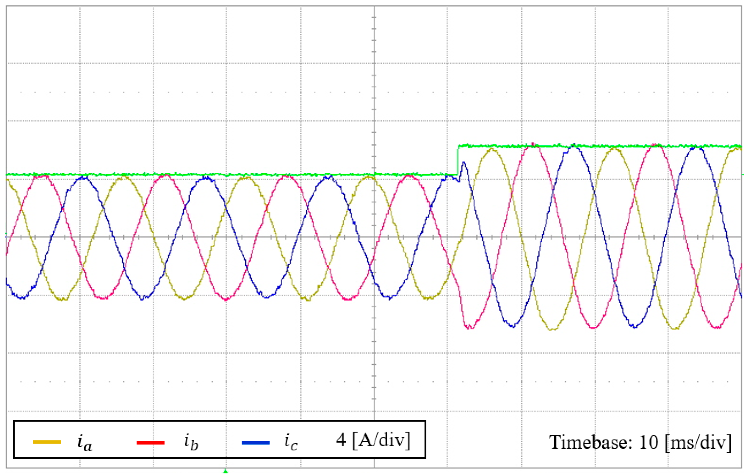
To demonstrate the grid disturbance rejection capability of the proposed control scheme, Figure 10 shows the transient response of the proposed scheme when there is a sudden change in the grid condition. The ideal grid voltages are suddenly distorted to the condition as in Figure 3 at 0.3 s. Even in this test condition, the proposed scheme yields a stable control performance except for a slight change in the THD value from 1.61% under the ideal grid to 1.67% under distorted grid, which proves the disturbance rejection capability of the proposed scheme. Through the comparative simulation results between the proposed scheme and the traditional ones, it is validated that the proposed scheme yields better current quality, while retaining a fast transient response.

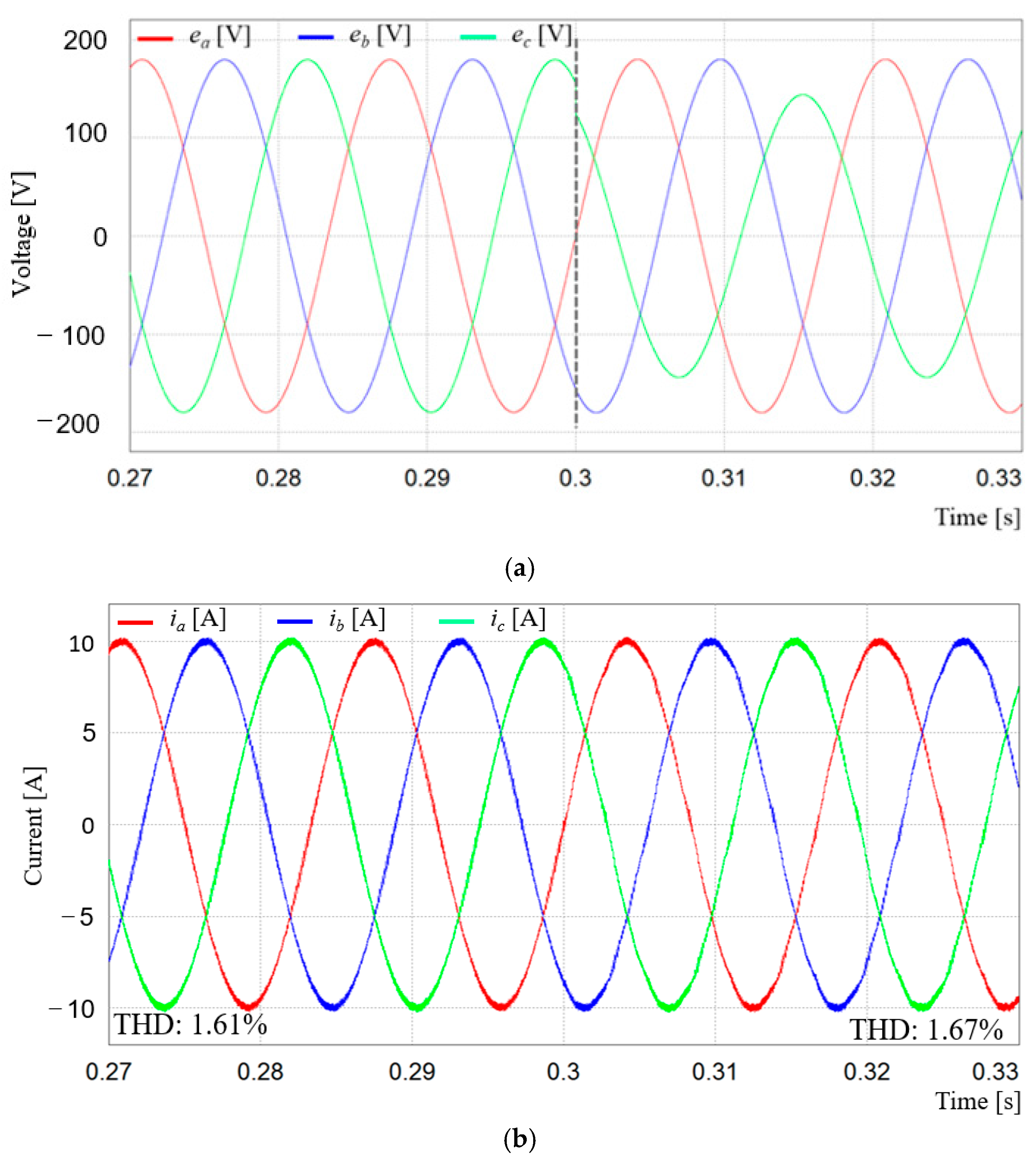
Figure 11 shows the transient response of the proposed FCS-MPC scheme when the ideal grid voltages are suddenly unbalanced at 0.3 s where c-phase grid voltage is reduced to 80% of the nominal grid voltages. As can be seen in these figures, the transient behavior of current between two grid conditions is stable and seamless except for a slight change in the THD value, which proves that the proposed scheme works effectively even under sudden unbalanced grid condition.

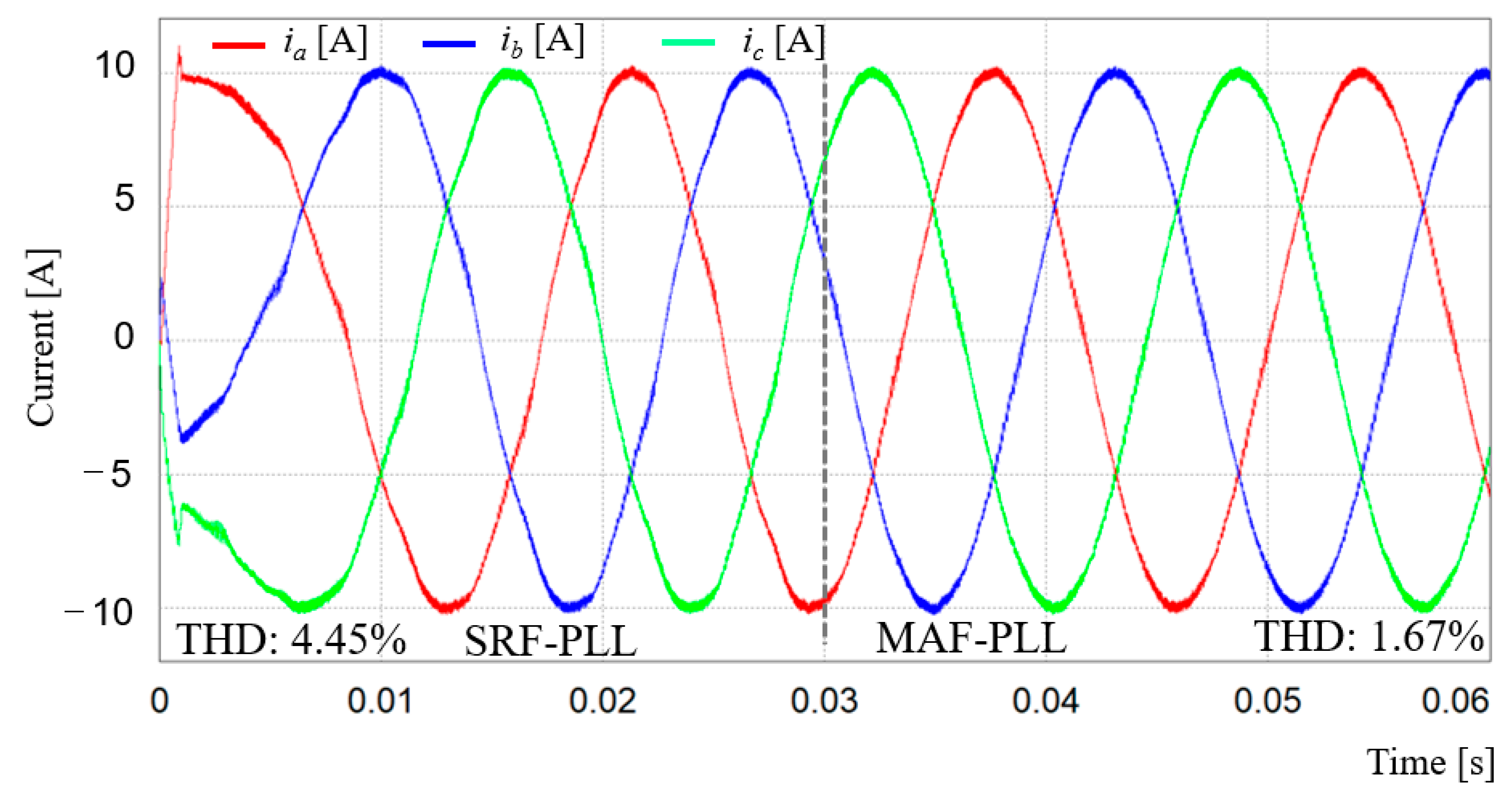
Figure 12 shows the improvement of the transient response through a modification of the proposed FCS-MPC scheme. Because the slow transient is mainly due to the adoption of the MAF, the modified method works with the FCS-MPC scheme and conventional SRF-PLL at start-up instant. Even though this structure does not give better performance than the proposed scheme in view of the THD value, the transient response is significantly improved as shown in Figure 12. As soon as the output currents reach the steady state, the control structure is changed to use the MAF-based PLL, resulting in the same THD value of the proposed scheme. When the transient response of current is a crucial concern, this modified control structure can be a good candidate to improve the transient response.

5. Experimental Results

5.1. Experimental Setup

In order to evaluate the feasibility of the proposed control method, the control algorithm is implemented on 32-bit floating-point DSP TMS320F28335 to control 2 kW prototype grid-connected inverter [24]. The configuration of the entire system is illustrated in Figure 13a. The sampling period is chosen as 100μs, which results in the switching frequency of 10 kHz. The inverter phase currents are detected using Hall effect sensors and converted through 12-bit A/D converter. An intelligent power module is employed for three-phase grid-connected inverter. A three-phase programmable AC power source is used to emulate the ideal grid as well as distorted grid conditions. Figure 13b depicts the photograph of the experimental test setup.

The whole control algorithm is implemented in C language program with the software environment of Code Composer Studio. The main control algorithm consists of the current prediction, the calculation of the cost function, the cost function minimization, and the MAF-PLL. In addition, the algorithm to operate the PWM and A/D converter is implemented. To execute the main control algorithm, about 40% of the sampling period is required. During this duration, the main control algorithm determines the duty intervals of two active voltage vectors which are applied to inverter in the next sampling period. These duty intervals of two active voltage vectors are implemented by using the internal enhanced PWM (ePWM) module of the DSP. In addition, to prevent shoot-through in the DC-link caused by the simultaneous conduction of both switches, the dead-time should be considered. This dead-time is implemented by using the built-in dead band generator module within the ePWM module.

5.2. Experimental Results

Figure 14 shows the distorted three-phase grid voltages used in the experiments. Similar to the simulations, these grid voltages contain the 5th and 7th harmonics with 10% of the fundamental component and the 11th and 13th harmonics with 1% of the fundamental component, respectively.

Figure 15 shows the inverter output current waveforms of the proposed control scheme under the ideal grid condition. It is shown that the proposed scheme operates well and produces comparable result with the conventional control schemes.

Figure 16 and Figure 17 show the experimental results for inverter output currents when the PI decoupling controller and the PR controller are employed under the distorted grid voltages as shown in Figure 14, respectively. Except for the difference in the THD value as a result of implementation in a real hardware system, all the experimental results well match with the simulation results. The phase current waveforms are quite distorted because these types of current controllers cannot effectively compensate the harmonic distortion caused by distorted grid voltages. The FFT results indicate that there exists relatively large quantity of unwanted harmonic contents in inverter output currents. The THD values of the PI control and the PR control are 6.3% and 4.3%, respectively.

Figure 18 shows the experimental results for the proposed control scheme under the same grid condition as the cases in the PI decoupling controller and the PR controller. Unlike the conventional schemes, the proposed scheme shows nearly sinusoidal current waveforms due to a good harmonic compensation capability as shown in Figure 18a. The FFT result shows that the harmonics in output currents are significantly reduced. The THD value of the proposed scheme is only 2.73%, which is considerably smaller than those of the PI and the PR controllers. Obviously, all the harmonic components are within the harmonic current regulation limit specified by IEEE std.1547.

The experimental result of the transient response for the proposed control scheme is shown in Figure 19. To evaluate the transient behavior of output current, the q-axis current reference is changed by step. As can be observed, the inverter output currents instantly reach a new steady-state, which demonstrates the fast transient response of the proposed scheme. Such a fast transient can be achieved by the fast nature of the MPC as well as the adoption of the MAF-PLL.

6. Conclusions

In this paper, an improved current control strategy for a three-phase grid-connected inverter based on a modulated FCS-MPC and MAF-PLL has been presented with the purpose of mitigating the harmonic components in inverter output currents when the grid is polluted by harmonic distortion. In terms of the performance, it is important for a grid-connected inverter to maintain the harmonic contents of inverter output currents below the specified limit even in the presence of harmonic-distorted grid. To consider the modulated FCS-MPC as an effective way of suppressing the harmonics in a grid-connected inverter under distorted grid, the proposed control scheme consists of several steps. First, the accurate system model in the discrete-time domain is developed to predict the future behavior of system. Based on the predicted output currents, both the generation of reference voltages and the calculation of duty intervals are accomplished. By using the information on the duty intervals as weighting factors, a cost function is determined by considering the control objective. Then, the cost function is minimized through the optimization process to determine the control signals for inverter.

In addition, for the purpose of improving the transient response, the MAF-PLL is employed to replace the traditional SRF-PLL. By using the MAF, the harmonic components caused by distorted grid voltages can be removed effectively and rapidly. This can contribute to generate the harmonic-free sinusoidal reference currents on the stationary reference frame, which is the vital part of mitigating the harmonic distortion in inverter currents. The principle and mathematical description of the proposed scheme have been analyzed to emphasize the simplicity of the control structure. The whole control algorithm has been implemented on a 32-bit floating-point DSP TMS320F28335 to control a 2 kW prototype grid-connected inverter. Comparative simulation and experimental results prove that the proposed scheme is an effective way to improve the performance of a grid-connected inverter under highly distorted grid voltages.