Optimization of Guide Vane Closing Schemes of Pumped Storage Hydro Unit Using an Enhanced Multi-Objective Gravitational Search Algorithm

Abstract

The optimization of guide vane closing schemes (OGVCS) of pumped storage hydro units (PSHUs) is a cooperative control and optimal operation research field in renewable energy power generation technology. This paper presents an OGVCS model of PSHUs considering the rise rate of the unit rotational speed, the specific node pressure of each hydraulic unit, as well as various complicated hydraulic and mechanical constraints. The OGVCS model is formulated as a multi-objective optimization problem to optimize conflicting objectives, i.e., unit rotational speed and water hammer pressure criteria. In order to realize an efficient solution of the OGVCS model, an enhanced multi-objective bacterial-foraging chemotaxis gravitational search algorithm (EMOBCGSA) is proposed to solve this problem, which adopts population reconstruction, adaptive selection chemotaxis operator of local searching strategy and elite archive set to efficiently solve the multi-objective problem. In particular a novel constraints-handling strategy with elimination and local search based on violation ranking is used to balance the various hydraulic and mechanical constraints. Finally, simulation cases of complex extreme operating conditions (i.e., load rejection and pump outage) of a ‘single tube-double units’ type PSHU system are conducted to verify the feasibility and effectiveness of the proposed EMOBCGSA in solving OGVCS problems. The simulation results indicate that the proposed EMOBCGSA can provide a lower rise rate of the unit rotational speed and smaller water hammer pressure than other methods established recently while considering various complex constraints in OGVCS problems.

1. Introduction

In recent years, in order to improve the global greenhouse effect and carbon dioxide emissions, the use of wind power, solar power generation, biomass energy and other renewable energy sources has been expanding to maintain China’s rapid development momentum [1,2]. Grid installed capacity and new energy power generation has continued to grow, which effectively alleviates the pressure on economic development of coal, oil and other fossil energy dependence, contributes to the energy structure reform and the development of green energy. It is estimated that by the year 2020, the installed wind power, photovotaic and pumped storage capacity will reach 210 million kW, 110 million kW and 100 million kW, respectively. However, wind energy and solar energy are intermittent resources, which exacerbates the contradiction between the development and utilization of new energy sources. As special energy storage power supplies, wind power-pumped storage plants (PSPs) and solar power-PSPs are the most commonly used centralized and large-scale renewable energy complementary operation means [3,4,5,6,7]. The flexibility of PSP makes up for the randomness and heterogeneity of wind power and solar power generation, which is helpful to improve the reliability of the power grid and promote the integration of renewable energy forms.

The OGVCS is an important means to solve the regulation and guarantee calculation of the pumped storage power plant, and is also the preferred method to optimize the hydraulic transient process. During the dynamic process of of PSHUs with the non-optimal closing law under extreme conditions (i.e., load rejection or pump outage), the rise of the unit rotational speed and the water hammer pressure will exceed the maximum design value, which can cause the runaway of the PSHU, abnormal vibrations or active guide vane asynchronous and other negative phenomena [8,9]. OGVCS plays an important role in ensuring the security and stability of the power grid, and several methods have been proposed to deal with the OGVCS problem. Based on the characteristics of the rigid water-column pressure during the transient process, [10] proposed a two-phase guide-vane closing scheme and three-phase valve-closing schemes to control the pulsating pressures and the runaway speed problems. Reference [11] analysed the effect of valve closure on the water-hammer pressure and laid the theoretical foundation for improving the turbine guide-vane closure. In order to avoid the operating point from being in the “S” characteristic area, Kuwabara et al. [12] proposed a curved closing scheme that could effectively decrease the water-hammer pressure. Additionally, appropriate two-phase closing schemes [13,14] and misaligned guide-vane methods [15,16,17] also have been applied to control the fluctuation of PSHUs. Three-phase valve-closing and curved closing schemes exert high demands on the governor servomotor, which is difficult to realize in a PSP. Meanwhile, the misaligned guide-vane method can significantly increase the pulsating pressure and the runner radial forces during the PSHU start-up process [17]. Therefore, optimal closing schemes are required to realize optimal coordinated operation of PSP and new energy generation technologies based on a deep analysis of the operational mechanism and flow characteristics of PSHUs.

Taking into full consideration the complex hydraulic, mechanical and electrical coupling characteristics and nonlinear dynamic response process of PSHUs, a multi-objective optimization model of guide vane closing schemes is established in this paper, which includes hydraulic and mechanical multiple constraint factors. The OGVCS problem is a complex, multi-objective and multi-constraint optimization problem, which aims to reasonably and simultaneously control the rotational speed and water hammer pressure of volutes, draft tubes, surge tanks and so on. Multi-objective intelligent optimization algorithms are an effective way to solve complex multi-objective problems, and many intelligent optimization algorithms, such as particle swarm optimization (PSO), gravitational search algorithm (GSA) and so on, are widely used in solving such multi-objective optimization problems. Multi-objective particle swarm optimization (MOPSO) [18,19], non-dominated sorting genetic algorithm-II (NSGA-II) [20], multi-objective differential evolution (MODE) [21,22], multi-objective gravitational search algorithm (MOGSA) [23,24] and multi-objective bee colony optimization algorithm (MOBCO) [25,26], have all been proposed to solve complex multi-objective optimization problems with practical and efficient modeling of coupling constraints. However, premature minimization phenomena and local convergence are still common obstacles to the performance of these stochastic searching algorithms. The so-called bacterial-foraging chemotaxis gravitational search algorithm (BCGSA) is enhanced by Pbest-Gbest-guided movement, adaptive elastic-ball method and the chemotaxis operator strategy of the bacterial-foraging algorithm [27]. The global exploration and local exploitation performance of BCGSA have been proved in [27]. Inspired by the NSGA-II, EMOBCGSA has been introduced to deal with the OGVCS by reconstructing the optimal structure and method. Finally, cases of complex extreme operating conditions of ‘single tube-double unit’-type PSHU systems are studied to verify the feasibility and effectiveness of the proposed EMOBCGSA in solving OGVCS problems.

The remainder of this paper is organized as follows. Section 2 introduces numerical calculation modeling of a “single tube-double unit”-type PSHU system. Section 3 establishes a multi-objective optimization model of guide vane closing schemes and multiple constraints are introduced simultaneously. Section 4 delineates the general procedure and multi-objective improvements in BCGSA. Section 5 illustrates the practical solving procedure for OGVCS problems and experimental results, along with a few discussions, respectively. The conclusions are summarized in Section 6.

2. Numerical Calculation Model of the Pumped Storage Hydro Unit System

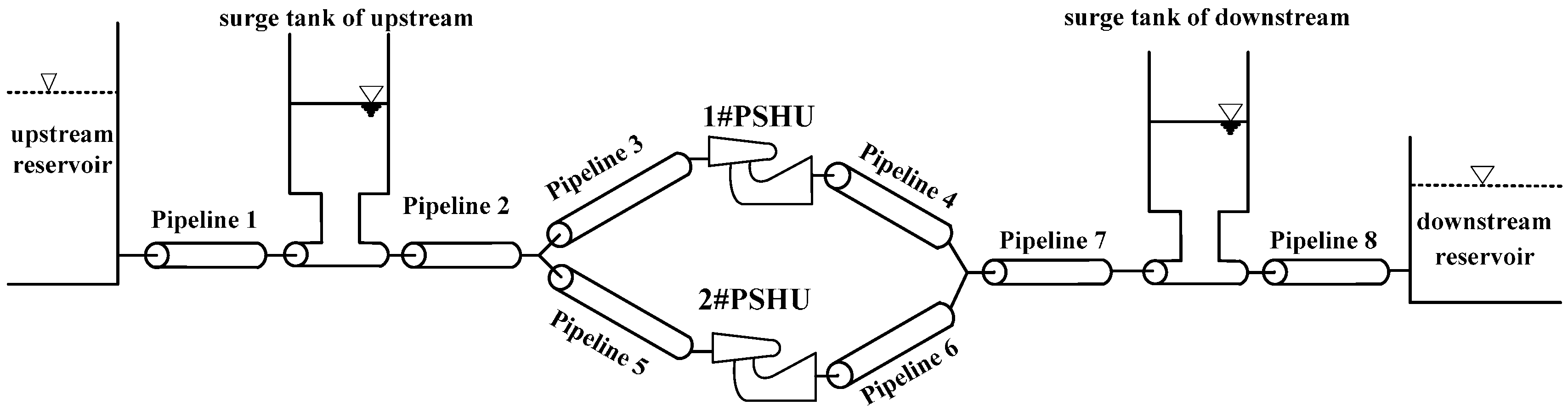
The “single tube-double unit”-type PSHU system is a typical kind of power generation system that couples hydraulic, mechanical and electrical factors, simplified mainly into four parts, namely reservoir, pressure water pipeline, surge tank and pumped storage hydro unit. Figure 1 shows a schematic diagram of the “single tube-double units”-type PSHU system used in this paper, where the PSHU system is divided into upstream and downstream reservoirs, eight pressure water pipelines, upstream and downstream surge tanks, and two PSHUs. In this section, mathematical models of each link are described.

2.1. Model of Pressure Water Pipeline

The well-known characteristics method is employed in the modeling of pressure water pipelines. The basic motion equation and continuous unsteady flow equation in a pressure pipeline can be expressed by Equations (1) and (2) [28]. Equations (1) and (2) can be solved using the method of characteristics, which transforms the formulas into a simplified equation set in the range of the characteristic line $\frac{dx}{dt}=\pm a$. The simplified equation set is described as by Equations (3) and (4):

$$\mathrm{Motion}\mathrm{equation}:\frac{\partial V}{\partial \mathrm{t}}+V\frac{\partial V}{\partial x}+g\frac{\partial H}{\partial x}+\frac{f}{2D}V|V|=0$$

(1)

$$\mathrm{Continuous}\mathrm{equation}:\frac{a^2}{g}\frac{\partial V}{\partial x}+V(\frac{\partial H}{\partial x}+\sin \alpha )+\frac{\partial H}{\partial t}=0$$

(2)

$$C^{+}:\{\begin{array}{l}\frac{dH}{dt}+\frac{a}{gA}\frac{dQ}{dt}+\frac{af}{2gD{A}^2}Q|Q|=0\\ \frac{dx}{dt}=a\end{array}$$

(3)

$$C^{-}:\{\begin{array}{l}\frac{dH}{\mathrm{dt}}-\frac{a}{gA}\frac{dQ}{dt}-\frac{af}{2gD{A}^2}Q|Q|=0\\ \frac{dx}{dt}=-a\end{array}$$

(4)

where $V$ is the flow velocity, $H$ is the piezometric head, a is the water hammer velocity, $f$ is the friction coefficient, $D$ is the pipeline diameter, $\alpha$ is the angle between the line and a horizontal surface of each section of the pipeline center, $V$ and $H$ are functions of the pipe length $x$ and time $t$, respectively, $A$ is the pipe section area, and $Q$ is the water flow in the pipe section.

The difference network is constructed using the above simplified equation set, then the finite difference method is used to solve the problem. Figure 2 shows the characteristic line difference mesh. For Figure 2, the length of $L$ pipeline is divided into $N$ segments, and the length of each segment is $\Delta x=L/N$, while the time step of the differential network is $\Delta t=\Delta x/a$.

Diagonal $AP$ satisfies the condition $\Delta x=a\Delta t$ and diagonal $BP$ satisfies the condition $\Delta x=-a\Delta t$. Equations (5) and (6) are the integral of motion equation between A and P and the integral of continuous equation between B and P, respectively:

$$(H_P-H_A)+\frac{a}{gA}(Q_P-Q_A)+\frac{f}{2gD{A}^2}{\displaystyle \underset{A}{\overset{P}{\int }}Q\left|Q\right|dx=0}$$

(5)

$$(H_P-H_B)-\frac{a}{gA}(Q_P-Q_B)-\frac{f}{2gD{A}^2}{\displaystyle \underset{B}{\overset{P}{\int }}Q\left|Q\right|dx=0}$$

(6)

Finally, the correct processing and analog computation of boundary conditions for the PSHU system in the transient process of the research and control are very important. The boundary conditions are a conduit or a connected terminal, including upstream reservoir, upstream surge tank, series nodes, bifurcated pipe nodes, ball valve, PSHU, downstream surge tank and downstream reservoir. Besides the surge tank and PSHU, the other boundary conditions as well as the spiral case and tail pipe usually can be considered as pressure water pipelines.

2.2. Surge Tank Model

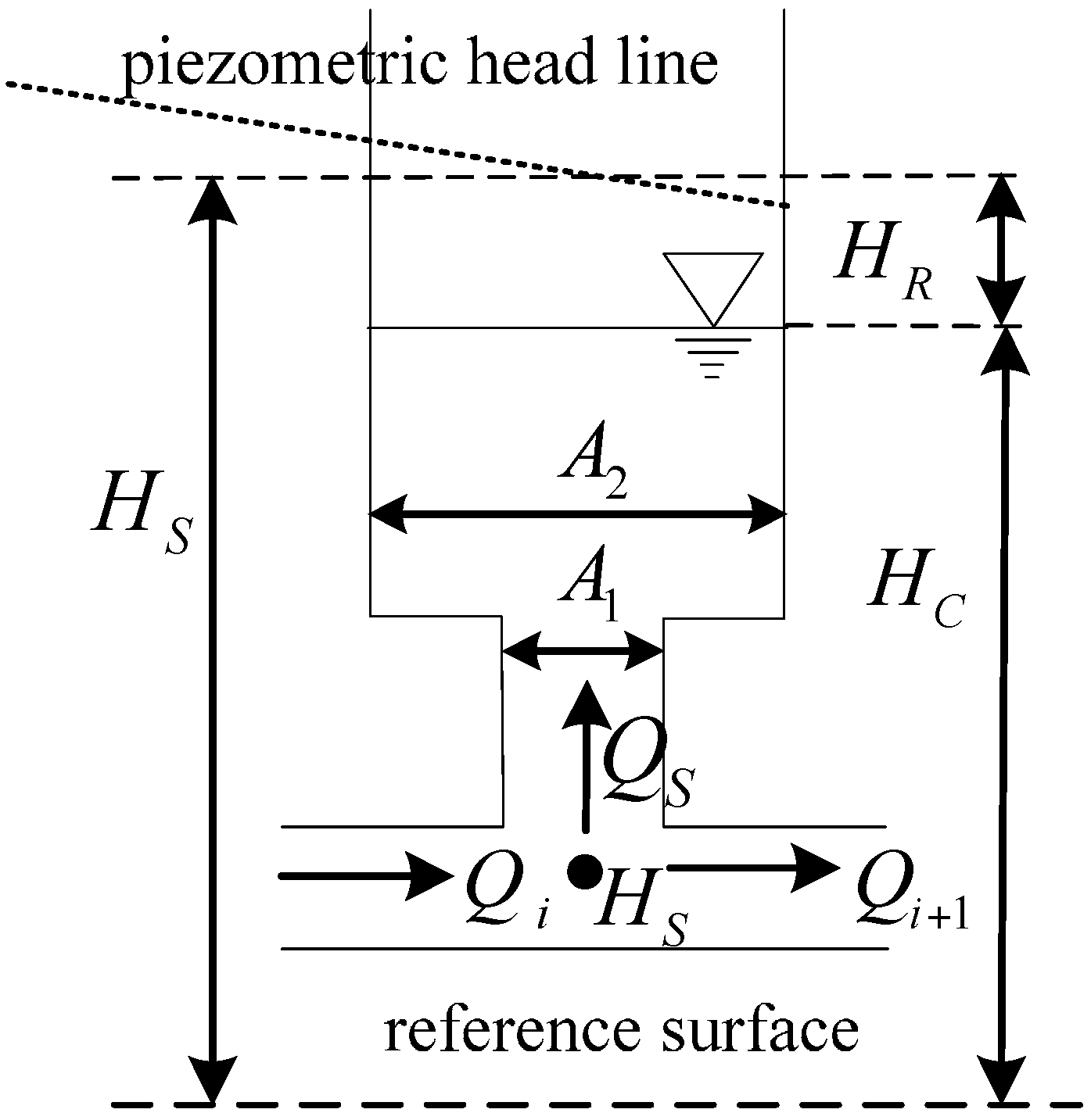
There are many types of surge tanks in the built pumped storage power stations, including impedance type, differential type and air cushion type. Based on the actual situation of pumped storage power stations in China, the impedance surge tank is adopted by the PSHU system in this paper. The schematic diagram of the impedance surge tank is shown in Figure 3, from which the impedance surge tank is connected with the water pipeline system through a small impedance orifice, which has the advantages of small volume and simple structure. The corresponding basic equations can be described by Equation (7) [29,30,31]:

$$\{\begin{array}{l}{H}_S=H_C+H_R\\ H_R=K_S\left|Q_S\right|Q_S\\ Q_S=A_2\frac{d{H}_C}{dt}\\ K_S=\frac{K_R(Q_S)}{2g{A}_1^2}\end{array}$$

(7)

where $H_S$, $Q_S$ are the surge tank bottom pressure and flow, $A_1$ is the area of the impedance orifice, $H_C$, $A_2$ are the elevation and area of the surge tank, $K_R$ is the bottom orifice flow loss coefficient.

2.3. Pumped Storage Hydro Unit Model

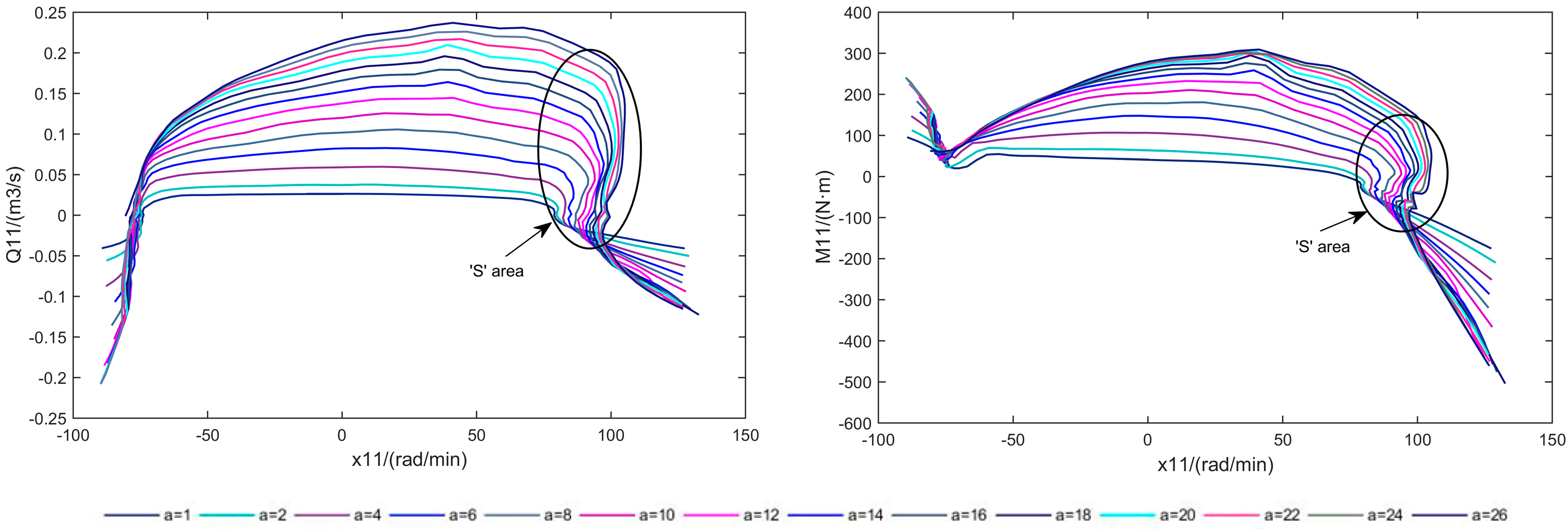
The PSHU is composed of a pump-turbine and generator, which are the key components of a PSHU system. At present, pump-turbine modeling based on the characteristic curves has been widely used. In this paper, the pump-turbine is expressed with the torque function and flow function for state variables, including guide vane opening, generator rotational speed and water head, shown as Equation (8) [32]. The analytic expressions of the nonlinear functions of $f_m(\cdot )$ and $f_q(\cdot )$ are difficult to obtain, however, based on the characteristic curves (Figure 4), torque and flow of the pump-turbine at a certain time can be calculated by means of interpolation or nonlinear function fitting. In order to overcome the obstacle of single input-multiple output during the interpolation calculation process, the logarithmic-curve-projection method is adopted for the mathematical transformation of the characteristic curves [33]:

$$\{\begin{array}{l}{m}_t=f_m(y,x,h)\\ q=f_q(y,x,h)\end{array}$$

(8)

where $m_t$ and $q$ indicate the torque and flow of the pump-turbine, respectively.

In this paper, only the PSHU rotational speed change of standalone running in the isolated power grid is considered [34]. The dynamic equation of the synchronous generator considering the load characteristics is simplified to give Equation (9):

$$\frac{x(s)}{mt(s)-m{g}_0(s)}=\frac{1}{T_{a}s+e_g}$$

(9)

where $x$ is the generator rotational speed, $T_a$ is the inertial time constant of the generator, $e_g$ is the adjusting coefficient of the generator, and $m{g}_0$ is the load disturbance which represents the load changes.

3. Optimization of Guide Vane Closing Schemes Problem Formulation

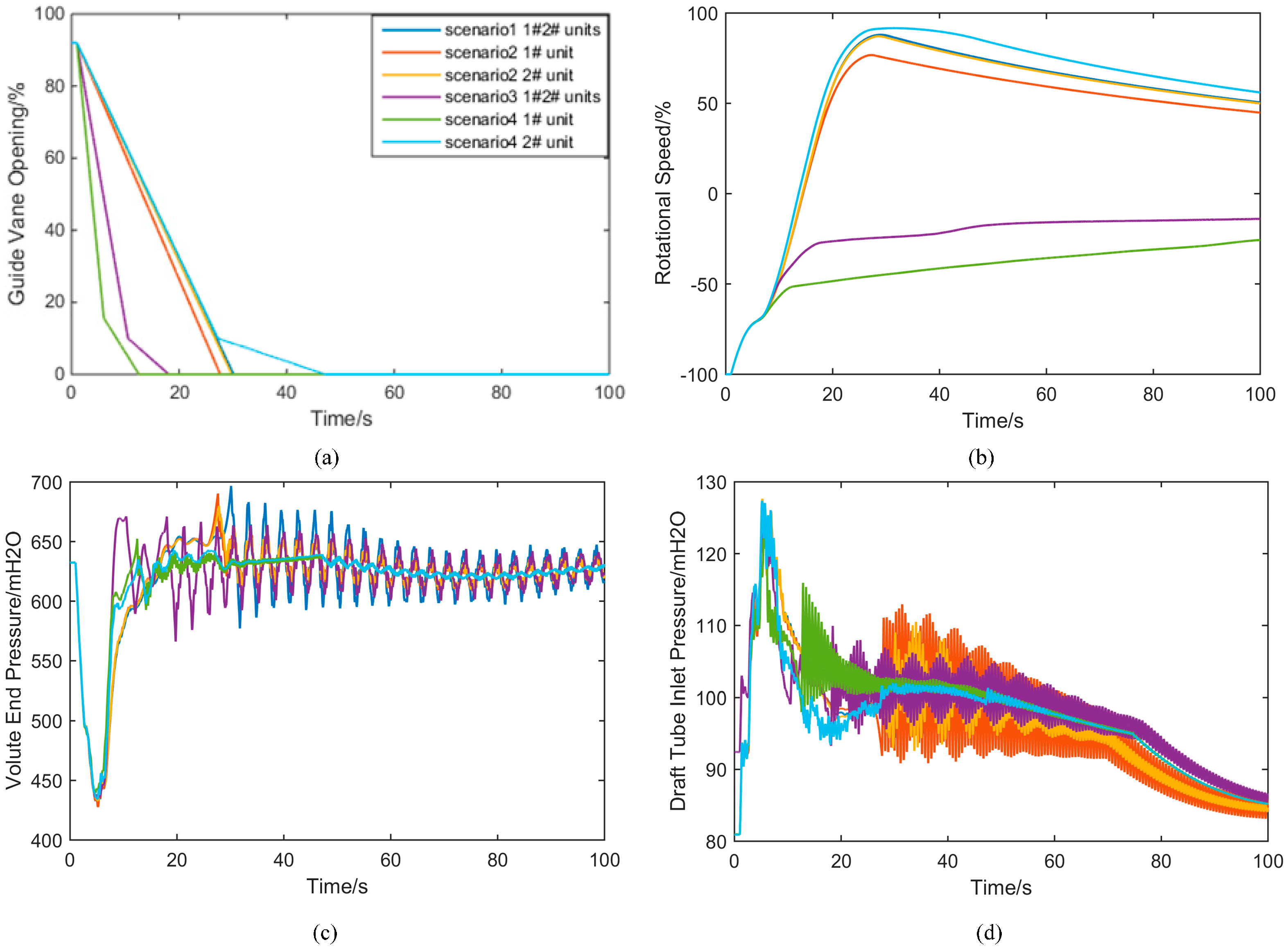
The dynamic response characteristics of the unit and the hydraulic influence of the large fluctuation condition of the PSHU are analyzed under the conditions of different guide vane closing laws. Considering the increase of unit rotational speed and pressure of each node in the hydraulic unit as the two objectives, the optimal model of the guide vane closing law is established.

3.1. Objective Function

3.1.1. Rotational Speed Objective

The rise of the rotational speed is one of the main characteristics of the pumped storage units under load rejection or pump power off conditions. Under load rejection conditions, a non-optimal guide vane closure law will lead to the runaway phenomenon, causing mechanical damage, vibrations and noise in the PSHU. The minimize rotational speed objective $Ob{j}_x$ of the OGVCS problem can be expressed as follows:

$$MinOb{j}_x={\displaystyle \sum _{i=1}^{N_{pu}}(\max (x_i)-}{x}_{r,i})/x_{r,i}$$

(10)

where $N_{pu}$ is the number of units in a hydraulic unit, $x_i$ is the rotational speed of $i$ unit during the transition process, $x_{r,i}$ is the rated rotational speed of the unit under stable conditions.

3.1.2. Water Hammer Pressure Objective

In order to minimize the pressure of each hydraulic unit, comprehensively considering the volute end pressure, tail pipe inlet pressure and surge tank water level value, the water hammer pressure objective function $Ob{j}_{pre}$ is established as follows:

$$MinOb{j}_{pre}=w_P\sum _{i=1}^{N_{pu}}(P_{vol\_e,i}+P_{dra\_s,i})+w_L(L_{sur\_up}+L_{sur\_down})$$

(11)

where $P_{vol\_e,i}$, $P_{dra\_s,i}$ are the maximum value of the volute end pressure and tail pipe inlet pressure for $i$ unit, $L_{sur\_up}$, $L_{sur\_down}$ are the maximum water level of the upstream surge tank and downstream surge tank, $w_P$, $w_L$ are the weight coefficients of the water hammer pressure and water level in the surge tank.

3.2. Multiple Constraints

The OGVCS problem should satisfy the following equality and inequality constraints:

(1) Rising rotational speed constraint

To guarantee regulation calculation and transient analysis of a PSHU system, there is a clear maximum constraint value $\mathrm{cons}{\mathrm{tant}}_x$ for the rise value of rotational speed in all kinds of extreme cases:

$$Ob{j}_{x,i}\le \mathrm{cons}{\mathrm{tant}}_x$$

(12)

(2) Limit of rotational speed fluctuation

In this paper, the limit of the times of rotational speed fluctuation is introduced in order to achieve a good dynamic quality of the large fluctuation condition process:

$$\{\begin{array}{l}{N}_{xf}={\displaystyle \sum num}(Ob{j}_{x,i}\ge \mathrm{cons}{\mathrm{tant}}_{ob{j}_{x_r}})\\ N_{xf}\le \mathrm{cons}{\mathrm{tant}}_{xf}\end{array}$$

(13)

where $\mathrm{cons}{\mathrm{tant}}_{ob{j}_{x_r}}$ is the rising rate constant for dynamic quality requirements, $N_{xf}$ is the number of fluctuations, and $\mathrm{cons}{\mathrm{tant}}_{xf}$ is constraint constant of the number of fluctuations.

(3) Volute pressure constraint

The maximum corrected value and the pressure constraint of the volute inlet pressure considering the pressure fluctuation and the calculation error are described as follows:

$$\{\begin{array}{l}P{m}_{vol\_s,i}=P_{vol\_s,i}+H_n\times 7\%+(P_{vol\_s,i}-P_{vol,i})\times 10\%\\ P{m}_{vol\_s,i}\le \mathrm{cons}{\mathrm{tant}}_{P{m}_{vol\_s}}\end{array}$$

(14)

where $P_{vol\_s,i}$, $P_{vol,i}$ and $P{m}_{vol\_s,i}$ are the maximum calculated value, initial value and maximum corrected value of the volute inlet pressure for $i$ unit, $H_n$ is the net head, and $\mathrm{cons}{\mathrm{tant}}_{P{m}_{vol\_s}}$ is the constraint constant of $P_{vol\_s,i}$.

(4) Draft tube inlet pressure constraint

$$\{\begin{array}{l}P{m}_{dra\_s,i}=P_{dra\_s,i}-H_n\times 3.5\%-(P_{dra,i}-P_{dra\_s,i})\times 10\%\\ P{m}_{dra\_s,i}\ge 0m\mathrm{conventional}\mathrm{condition}\\ P{m}_{dra\_s,i}\ge -5m\mathrm{successive}\mathrm{load}\mathrm{rejection}\end{array}$$

(15)

where $P_{dra\_s,i}$, $P_{dra,i}$ and $P{m}_{dra\_s,i}$ are minimum calculated value, initial value and minimum corrected value of the draft tube inlet pressure for $i$ unit.

(5) The surge water level limits

$$\{\begin{array}{l}{L}_{sur\_up}\le \mathrm{cons}{\mathrm{tant}}_{L_{sur\_up}}\\ l_{sur\_up}\ge \mathrm{cons}{\mathrm{tant}}_{l_{sur\_up}}\\ L_{sur\_down}\le \mathrm{cons}{\mathrm{tant}}_{L_{sur\_down}}\\ l_{sur\_down}\ge \mathrm{cons}{\mathrm{tant}}_{l_{sur\_down}}\end{array}$$

(16)

where $L_{sur\_up}$ and $l_{sur\_up}$ are the maximum and minimum values of the surge water level of the upstream surge tank, $L_{sur\_down}$ and $l_{sur\_down}$ are maximum and minimum values of the surge water level of the downstream surge tank, and the other terms are the corresponding constraint constants.

(6) Speed governor oil velocity limit

If the guide vanes are closed within a short time, the control accuracy of the governor curve slope has higher requirements. In order to meet such a short closing time demand, the servomotor oil speed must be large enough, which can cause major safety issues. Therefore, this paper takes into account the limiting factor of the slope control of the governor and transforms it into the guide vane closing rate:

$$\Delta Y/t\le Y\_\max /Tr$$

(17)

where $\Delta Y$ and $Y\_\max$ are change value and rated maximum value guide vane opening, $t$ is the guide vane closing time, and $Tr$ is the minimum closing time limit.

4. Enhanced Multi-Objective Bacterial-Foraging Chemotaxis Gravitational Search Algorithm Methodology

4.1. Overview of Bacterial-Foraging Chemotaxis Gravitational Search Algorithm

BCGSA is an improvement of the standard gravitational search algorithm (GSA) by incorporating the P_best-G_best-guided movement, adaptive elastic-ball method and chemotaxis operator strategies. Then the specific steps of BCGSA are as follows:

Step 1:

Initialization. Randomly initialize the agent of population position and velocity.

Step 2:

Fitness calculation and information save. Calculate the fitness of agents according to their initial position, storing the current position of each agent P_best(t) as the best record position of the agent and position of best agent G_best(t) as the best position in global.

Step 3:

Update best(t), worst(t), and M_i(t) for i = 1, 2, …, N.

Step 4:

Calculate the gravitational constant in the current iteration and acceleration for each agent.

Step 5:

Update agents’ velocity $v_i^d$ and position $x_i^d$ with equations (18) and (19) [35].

$$v_i^d(t+1)=r_1\cdot v_i^d(t)+a_i^d(t)+c_1\cdot r_2\cdot (P_{ibest}^d(t)-x_i^d(t))+c_2\cdot r_3\cdot (G_{best}^d(t)-x_i^d(t))$$

(18)

$$x_i^d(t+1)=x_i^d(t)+v_i^d(t)$$

(19)

where $r_1$, $r_2$ and $r_3$ are random variables in the range [0, 1], $c_1$ and $c_2$ are learning genes in the range [0, 2], $P_{ibest}(t)$ is the best position that i-th agent has ever suffered until time t, $G_{best}(t)$ is the global best position in the agents until time t.

Step 6:

Judge whether the new position of the agent is beyond the boundary. Invoke the adaptive elastic-ball program (Equation (20)) to handle the new position which is against the boundary. Besides, there are a few rest agents against the boundary whose position will be reset by Equation (21) [36]:

$$\{\begin{array}{l}if{x}_i^d(t)>Ub(d),up=x_i^d(t)-Ub(d)\mathrm{and}{x}_i^d(t)=Ub(d)-\zeta \cdot up\\ if{x}_i^d(t)<Lb(d),down=Lb(d)-x_i^d(t)\mathrm{and}{x}_i^d(t)=Lb(d)+\zeta \cdot down\end{array}$$

(20)

$$x_i^d(t)=rand\cdot (Ub(d)-Lb(d))+Lb(d)$$

(21)

where $\zeta$ is the adaptive attenuation coefficient of reflective power, $Ub(d)$ and $Lb(d)$ are upper and lower boundary limit in the d-th dimension, respectively.

Step 7:

Evaluate the fitness in accordance with the new position of each agent, storing position of the best agent $X^{best}$ and the worst agent $X^{worst}$ in the current iteration.

Step 8:

The chemotaxis operator [37] is applied for $X^{best}$ and $X^{worst}$.

(a)

Initialize parameters Nc, Ns and C(i). Where Nc is the number of chemotaxis steps, Ns is the number of swim steps.

(b)

Tumble. Generate a random vector Δ(i) $\in$ R^D with each element Δ_d(i), d = 1, 2, 3, …, D, a random number on [−1, 1].

(c)

Move. Define unit length random direction $\varphi (j)$ in j-th chemotaxis, then updates the best agent $X^{best}=[x_1^{best},x_2^{best},\dots ,x_d^{best},\dots ,x_D^{best}]$ and worst agent $X^{worst}=[x_1^{worst},x_2^{worst}\dots ,x_d^{worst},\dots ,x_D^{worst}]$ according to Equations (22) and (23).

$$\varphi (j)=\frac{\Delta (i)}{\sqrt{{\Delta }^T(i)\Delta (i)}}$$

(22)

$$x(i,j+1)=x(i,j)+C(i)\varphi (j)$$

(23)

where X^best is the agent of the best fitness, X^worst is the agent of the worst fitness, x(i, j) is the position of the i-th agent in the j-th chemotaxis.

(d)

Swim. Compute fitness of obtained new agent $x(i,j+1)$, then compare $fitness(i,j+1)$ and $fitness(i,j)$. If the $fitness(i,j+1)$ is better, save the new agent as $X_{new}^{best}$ or $X_{new}^{worst}$ and start agent swimming, then let m = 0 and repeat Equation (23) following this tumble direction until m = Ns; else let n=Ns directly, this is the end of the while statement.

(e)

Repeat (a)–(d) until Nc reaches the stop criteria. Replace G_best and G_worst by $X_{new}$, only when $X_{new}^{best}$ and $X_{new}^{worst}$ are better.

Step 9:

Compare the obtained fitness of a new position $x_i(t+1)$ with fitness of $P_{ibest}(t)$ and $G_{best}(t)$ while i changes from 1 to N. If $x_i(t+1)$ has a better fitness value, replace position of $P_{ibest}(t)$ and $G_{best}(t)$ by $x_i(t+1)$.

Step 10:

Repeat Steps 3–9 until the stop criterion is reached.

4.2. The Basic Definition of Multi-Objective Optimization Problem

Generally, the multi-objective minimize optimization problem of $n$ dimensions decision variable and $m$ dimensions subunit objectives can be described as follows:

$$\{\begin{array}{l}y=\mathrm{Min}F(x)=\{\min f_1(x),\min f_2(x),\dots ,\min f_m(x)\}\\ subjectto{g}_j(x)\ge 0(j=1,2,\dots ,J)\\ h_k(x)=0(k=1,2,\dots ,K)\\ x=(x_1,x_2,\dots ,x_n)\end{array}$$

(24)

where $[f_1,f_2,\dots ,f_m]$ are $m$ dimensions of objective vectors, $F(x)$ is a mapping function from decision space to object space, $g_j(x)\ge 0(j=1,2,\dots ,J)$ defines the $J$ inequality constraints, $h_k(x)=0(k=1,2,\dots ,K)$ defines the $K$ inequality constraints, $x=(x_1,x_2,\dots ,x_n)$ is the $m$ dimensions decision variable space.

Due to the conflictive relationship among multiple subobjectives, a set of non-dominated solutions exist rather than only one optimal solution. Thus, the key concept of Pareto optimality [38,39] associated with the trade-off between conflictive objectives is adopted:

(1) Pareto dominance relation

$X_f$ is a feasible solution set, $x_1$ and $x_2$ are feasible solutions, $[x_1,x_2]\in X_f$, if $x_1$ dominates $x_2$, note as $x_1\succ x_2$, if and only if:

$$\{\forall k=1,2,\dots ,m|f_k(x_1)\le f_k(x_2)\}\wedge \{\exists l\in (1,2,\dots ,m)|f_l(x_1)<f_l(x_2)\}$$

(25)

(2) Pareto optimal solution

For a given multi-objective optimal problem, if $x^{*}\in X_f$ is the Pareto optimal solution, if and only if:

$$\neg \exists x\in X_f:x\succ x^{*}$$

(26)

(3) Pareto optimal solution set

The set of all Pareto optimal solutions is called the Pareto optimal solution set $P^{*}$:

$$P^{*}=\left\{x^{*}\right|\neg \exists x\in X_f:x\succ x^{*}\}$$

(27)

(4) Pareto optimal front

The Pareto optimal solution set corresponding to the objective vector value in the objective domain space is called the Pareto optimal front $P{F}^{*}$:

$$P{F}^{*}=\{F(x^{*})=\{f_1(x^{*}),f_2(x^{*}),\dots ,f_m(x^{*})\}$$

(28)

4.3. Enhanced Multi-Objective Bacterial-Foraging Chemotaxis Gravitational Search Algorithm

The BCGSA is based on the single objective optimization design, which does not have the ability to deal with multi-objective optimization problems. Therefore, based on the BCGSA, this section reconstructs the optimal structure and mechanism of solving multi-objective optimization problems.

4.3.1. Population Reconstruction

In dealing with multi-objective optimization problems, it is more complex to determine the non-inferiority relation among population individuals and it is the key to improve the efficiency and ergodicity of the algorithm to establish a reasonable non-inferiority relation among individuals. Therefore, this paper further introduces a fast non-dominated sorting method, the crowding-distance concept, and then completes the whole population structure reconstruction.

(1) Non-dominated sorting

In order to realize the distribution and diversity of population of the BCGSA algorithm in dealing with multi-objective optimization problems in this group, inspired by NSGA-II [20], the fast non-dominated sorting method is applied to divide the population into a number of levels, the specific steps are as follows:

Step 1:

If any individual $x_i^d$ is not dominant in the current population, the individual is Pareto non-dominated, then its layer rank is 1, and all the individuals in the rank = 1 constitute the Pareto optimal front.

Step 2:

In the whole population, the individuals of rank = 1 are excluded; then repeat Step 1 until obtain the individual solution set of the second layer, and the individual attributes of the rank = 2 are given.

Step 3:

By analogy, repeat Step 2 until the completion of the entire population of non- dominated type. Assuming that the population size is 7, the objective number is 2, and the layering schematic is shown in Figure 5.

(2) Crowding-distance calculation

Crowding-distance is an important index to evaluate the distribution density of solution space, which can be described as follows:

$$\mathsf{\Gamma }{[p]}_{distance}=\{\begin{array}{l}{\displaystyle \sum _{l=1}^L{[(f_{p-1,l}-f_{p+1,l})/(f_l^{\max }-f_l^{\min })]}^2,p\in [2,Nr-1]}\\ {\displaystyle \sum _{l=1}^{L}2{[(f_{1,l}-f_{2,l})/(f_l^{\max }-f_l^{\min })]}^2,p=1}\\ {\displaystyle \sum _{l=1}^{L}2{[(f_{Nr-1,l}-f_{Nr,l})/(f_l^{\max }-f_l^{\min })]}^2,p=Nr}\end{array}$$

(29)

where $\mathsf{\Gamma }{[p]}_{distance}$ is the crowding-distance of individual $p$, $f_{p,l}$ is the fitness of objective $l$ of individual $p$, $L$ is the number of objective, $f_l^{\max }$ and $f_l^{\min }$ are the maximum and minimum fitness for individuals in each layer of the $L$ dimensional objective.

Thus, each individual consists of two attributes: the layer number and the crowding-distance. Depending on these two attributes can be defined between individual preference relations. $i$ is superior to $j$, if and only if:

$$\{\begin{array}{l}rank(i)<rank(j)\\ rank(i)=rank(j),\mathsf{\Gamma }{[i]}_{distance}>\mathsf{\Gamma }{[j]}_{distance}\end{array}$$

(30)

(3) Individual quality calculation

For EMOBCGSA, the quality of the individual cannot be calculated based on the value of the objective function, but it is obtained by the rank of the non-dominated layer number. For $l$ objective functions of multi-objective optimization problem, the calculation process of individual quality is given as follows:

Step 1:

In the rank = 1, the fitness values of the individuals with the smallest value of $l$ objective functions and the maximum crowding-distances are set to 1, and the fitness value of other individuals is 2.

Step 2:

In the rank = 2, set all the individual fitness values to 3.

Step 3:

Repeat Step 2, individual fitness value of $rank\ge 3$ is set to $(rank+1)$, thus completing all layers of individual fitness assignment.

Step 4:

Calculate the individual quality using Equation (31):

$$\{\begin{array}{l}{m}_i(t)=\frac{fi{t}_i(t)-worst(t)}{best(t)-worst(t)}\\ M_i(t)=\frac{m_i(t)}{{\displaystyle {\sum }_{j=1}^N{m}_j(t)}}\end{array}$$

(31)

4.3.2. Multi-Objective Adaptive Chemotaxis Operation

For multi-objective adaptive chemotaxis operations, the selections of $G_{best}$ and $G_{worst}$ are the key to speeding up the convergence of EMOBCGSA. In order to avoid the premature convergence and maintain the diversity of the population, the concept of constraint violation, as shown in Equation (32), is introduced in the selection process. Combined with individual crowding-distance, the probability of individual selection in rank = 1 and rank = max is calculated by Equation (33). By means of Equations (32) and (33) to adaptively calculate the probability of individual selection, then the tracking targets ($G_{best}$ and $G_{worst}$) of multi objective chemotaxis operation are determined by the roulette wheel method:

$$voilatio{n}_s=\{\begin{array}{l}{\displaystyle \sum _{ic=1}^{nc}\frac{valu{e}_{ic}-L{u}_{ic}}{L{u}_{ic}-L{d}_{ic}}valu{e}_{ic}\ge L{u}_{ic}}\\ {\displaystyle \sum _{ic=1}^{nc}\frac{L{d}_{ic}-valu{e}_{ic}}{L{u}_{ic}-L{d}_{ic}}valu{e}_{ic}\le L{d}_{ic}}\end{array}$$

(32)

$$p_s=\{\begin{array}{cc}Sp1\times \frac{1/voilatio{n}_s}{{\displaystyle \sum _{v=1}^{N_v}1/voilatio{n}_v}},\hfill & i\mathrm{f}voilatio{n}_s>\epsilon \hfill \\ Sp2\times \frac{\mathsf{\Gamma }{[s]}_{distance}}{{\displaystyle \sum _{d=1}^{N_d}\mathsf{\Gamma }{[d]}_{distance}}},\hfill & \mathrm{otherwise}\hfill \end{array}$$

(33)

where $voilatio{n}_s$ is the constraint violation of individual $s$, $valu{e}_{ic}$ is the value of $s$ in $ic$ constraint, $L{u}_{ic}$ and $L{d}_{ic}$ are the upper and lower limits of constraint $ic$, $nc$ is the number of constraints; $p_s$ is the selection probability of $s$, $\epsilon$ is the feasible margin of constraint failure depth evaluation (if $voilatio{n}_s>\epsilon$, and individual $s$ is infeasible solution), $N_v$ and $N_d$ are the number of infeasible solutions and feasible solutions, $Sp1$ and $Sp2$ are the initial selected probability constants of the infeasible and feasible solutions.

4.3.3. Multi-Objective Velocity Update Strategy

For the velocity update Equation (18) of EMOBCGSA, $G_{best}$ and $P_{best}$ need to be redefined when dealing with multi-objective problems. The selection mechanism of $G_{best}$ has been introduced in detail in Section 4.3.2, and $P_{ibest}^d(t)$ is the location of the optimal memory of the individual $i$ on the $d$ dimension of the $t$^th generation. The selection method of $P_{best}$ can be carried out according to Equation (30).

4.3.4. The Update and Maintenance of the Elite Archive Set

The elite archive set (EAS) is used to store the non-dominated solutions obtained during EMOBCGSA evolution, and provide guidance for the evolution of a population. In the actual operation of the algorithm, the newly generated individual $n{p}_s^g$ and the original individual $p_s^g$ are added to EAS when $n{p}_s^g$ and $p_s^g$ are mutually reciprocal domination. EAS update and maintenance strategies are performed as follows ($NQ$ is the capacity of EAS):

(1)

If the current capacity of EAS is zero, the elite candidates are added directly to the EAS.

(2)

If the EAS is not empty, and the elite candidate is not dominated by any elite individual in the original EAS, the elite candidate is added to the EAS. At the same time, the initial elite individual who is dominated by the candidate elite is removed from the EAS.

(3)

If the number of elite individuals stored in EAS has exceeded $NQ$, the EliteSet truncation method is used to maintain it.

All the individuals will be selected by the non-dominated sorting, and the first $NQ$ individuals with larger crowding-distance will be stored in EAS, where the redundant individuals will be removed.

4.3.5. Performance Test of Enhanced Multi-Objective Bacterial-Foraging Chemotaxis Gravitational Search Algorithm

In order to verify the performance of the EMOBCGSA in dealing with multi-objective problems, the test function set of ZDT is selected to test and evaluate the performance of the proposed algorithm [40]. In addition, the convergence and diversity indexes are introduced to evaluate the performance of the algorithm, respectively, such as Equations (34) and (35).

$$\gamma =\frac{1}{N}{\displaystyle \sum _{x=1}^N\{\Vert x-x^{\prime }\Vert ,x^{\prime }\in Z^{\prime }\}}$$

(34)

$$\psi =\frac{d_b+d_e+{\displaystyle \sum _{i=1}^{N-1}|d_i-\overline{d}|}}{d_b+d_e+(N-1)\overline{d}}$$

(35)

where N is the size of the Pareto solution set, $x$ is the arbitrary nondominated solution of the Pareto solution set, $x^{\prime }$ is the nearest pairing solution from the $x$ on the real Pareto front, $d_i$ is the Euclidean distance between two consecutive non-dominated solutions, $\overline{d}$ is the average value of all $d_i$, $d_b$ and $d_e$ respectively show that the algorithm obtains the Euclidean distance between the ends of the Pareto solution and the real Pareto front.

The convergence and diversity index of the test function set are calculated, and the results are compared with those of NSGA-II, MOPSO and multi objective evolutionary algorithm (MOEA). The mean and variance of the two indexes after the algorithms were run 20 times are shown in

Table 1. Convergence index.

	Method	NSGA-II	MOPSO	MODE	EMOBCGSA
Function
ZDT1	Mean value	0.036472	0.028287	0.017245	0.001533
	Variance	0.004750	0.000385	0.000385	0
ZDT2	Mean value	0.092391	0.197620	0.004203	0.000642
	Variance	0.035699	0.000915	0.000357	0
ZDT3	Mean value	0.114500	0.118409	0.012741	0.000057
	Variance	0.007940	0.00643	0.00112	0
ZDT4	Mean value	0.313023	2.926100	0.1001	0.002049
	Variance	0.068460	1.705000	0.3465	0.000288
ZDT6	Mean value	0.206564	0.242501	0.001624	0.000022
	Variance	0.010133	0.003245	0.00026	0

and

Table 2. Diversity index.

	Method	NSGA-II	MOPSO	MODE	EMOBCGSA
Function
ZDT1	Mean value	0.210307	0.254723	0.322890	0.052796
	Variance	0.000976	0.001874	0.001335	0.000039
ZDT2	Mean value	0.428778	0.345050	0.32160	0.042721
	Variance	0.004451	0.001965	0.001035	0.000083
ZDT3	Mean value	0.73440	0.433100	0.522340	0.426762
	Variance	0.018756	0.005165	0.041200	0.000039
ZDT4	Mean value	0.302610	0.634901	0.333600	0.042253
	Variance	0.004646	0.002243	0.162000	0.000069
ZDT6	Mean value	0.348025	0.944120	0.330100	0.07331
	Variance	0.003923	0.138106	0.033000	0.000209

. From Table 1, we can see that the EMOBCGSA test results are better than those of the other methods in convergence index, mean and variance, and the algorithm has strong convergence and robustness. In the distribution of diversity of non-dominated solutions, the results of EMOBCGSA in Table 2 are superior to the other optimization algorithms in terms of diversity index, mean and variance. The variance is small, and the calculation results are also stable.

5. Numerical Experiments and Analysis

5.1. Proposed Enhanced Multi-Objective Bacterial-Foraging Chemotaxis Gravitational Search Algorithm Approach for Optimization of Guide Vane Closing Schemes Problem

Depending on the mathematical description of the optimization objectives and constraints, OGVCS is a multi-objective optimization problem with multiple variables and multiple nonlinear constraints. The objectives and constraints involve a lot of hydraulic and mechanical factors, so it is important to have an efficient algorithm to solve the problem. In this section, the procedure of the proposed EMOBCGSA for solving OGVCS problems with complex constraints is described, and the corresponding constraints-handling strategy will be discussed later. The generalized procedure can be given as follows.

5.1.1. Population Initialization

At present, the common guide vane closing mode is straight line closure, two segment type broken line closure and three segment delay broken line closure. Because the governor of PSHU does not have the function of delay in the pump condition, this paper does not consider the three segment closing law. Figure 6 shows the schematic diagram of the straight line closure and the broken line closure.

From Figure 6, $T$ and $[Tf,Y,Tt]$ are the decision variables of the two kinds of closing law, respectively. Taking the broken line closure as an example and assuming that the optimized ‘single tube-$N_{PT}$ units’ type PSHU system, the individual $a$ can be constructed as matrix $U_a$ with $3\times N_{PT}$, $U_a$ is described as Equation (36), $Np$ is the size of population. Individuals can be randomly initialized by Equation (37):

$$U_a=\left[\begin{array}{llllll}T{f}_{1,1}\hfill & T{f}_{1,2}\hfill & \dots \hfill & T{f}_{1,n}\hfill & \dots \hfill & T{f}_{1,N_{PT}}\hfill \\ Y_{2,1}\hfill & Y_{2,2}\hfill & \dots \hfill & Y_{2,n}\hfill & \dots \hfill & Y_{2,N_{PT}}\hfill \\ T{t}_{3,1}\hfill & T{t}_{3,2}\hfill & \dots \hfill & T{t}_{3,n}\hfill & \dots \hfill & T{t}_{3,N_{PT}}\hfill \end{array}\right],a=1,2,\dots ,Np$$

(36)

$$\{\begin{array}{l}T{f}_{1,n}=T{f}_{1,n}^{\min }+rand(0,1)\times (T{f}_{1,n}^{\max }-T{f}_{1,n}^{\min })\\ Y_{1,n}=Y_{1,n}^{\min }+rand(0,1)\times (Y_{1,n}^{\max }-Y_{1,n}^{\min })\\ T{t}_{1,n}=T{t}_{1,n}^{\min }+rand(0,1)\times (T{t}_{1,n}^{\max }-T{t}_{1,n}^{\min })\end{array}n=1,2,\dots ,N_{PT}$$

(37)

where $T{f}_{1,n}^{\max }$ and $T{f}_{1,n}^{\min }$ are the upper and lower limits of $Tf$, $Y_{1,n}^{\max }$ and $Y_{1,n}^{\min }$ are the upper and lower limits of $Y$, $T{t}_{1,n}^{\max }$ and $T{t}_{1,n}^{\min }$ are the upper and lower limits of $Tt$.

5.1.2. Constraint-Handling Strategy

In this section, based on the concept of constraint violation, a novel constraints-handling strategy with elimination and local search based on violation ranking is proposed. The constraint-handling strategy is used to balance the various hydraulic and mechanical constraints of the OGVCS problem. The speed governor oil velocity limit of the governor can be dealt with after the initialization and updating of the individual, and the additional constraint is to judge whether the individual has violated the constraint condition after the OGVCS problem is solved. Therefore, the constraint-handling strategy can be divided into two parts: pre-correction and post-correction.

(1) Pre correction

Pre-repair is mainly aimed at tackling the speed governor oil velocity constraints. The processing steps are as follows:

Step 1:

For individual $i$, calculate the closing rate for each segment $\Delta Y/t$, judge the relationship between $\Delta Y/t$ with the rated closing rate $Y\_\max /Tr$.

Step 2:

If $\Delta Y/t>Y\_\max /Tr$, the closing rate of the guide vanes assigned to this segment is $Y\_\max /Tr$, reverse calculation closing time $t\_new$, then replace $t$ with $t\_new$.

Step 3:

Repeat Steps 1 and 2, until all of the individuals constraints have been repaired.

(2) Post-correction

The OGVCS problem is solved by the individuals who have been pre-repaired. According to the calculation value of the transient process of each hydraulic unit of PSHU system and Equation (32), we can calculate the total amount of constraint violation $voilatio{n}_i$. If $voilatio{n}_i\ne 0$, according to eliminate and local search strategy based on violation ranking for post repair, detailed steps are as follows:

Step 1:

Conduct a descending sort for individuals of $voilatio{n}_i\ne 0$.

Step 2:

Introduce coefficient $Cv$ of constraint violation, if $voilatio{n}_i<Cv$, start the local iterative search procedure. Then, randomly generated $\Delta y_i$, and the position of the inflection point of two segment type broken line closures is updated to $Y_i+\Delta y_i$, and we calculate the OGVCS problem. Repeat the above local iterative search procedure until $voilatio{n}_i=0$ or the required local search steps are met.

Step 3:

Repeat Step 1, complete local iterative search for individuals who are $voilatio{n}_i<Cv$, eliminate individuals who is $voilatio{n}_i\ne 0$.

5.1.3. Outline of Enhanced Multi-Objective Bacterial-Foraging Chemotaxis Gravitational Search Algorithm for Solving Optimization of Guide Vane Closing Schemes Problems

The process of OGVCS problem solving with EMOBCGSA is described as follows, and the flowchart is illustrated in Figure 7:

Step 1:

Set guide vane closing mode and corresponding parameters; initialize the control parameters $[NQ,Np,G_{\max },G_0,\beta ,c_1,c_2,Nc,Ns]$ of the EMOBCGSA, set the evolutionary current algebra $g=1$.

Step 2:

According to Equations (34) and (35) construct and initialize the individuals of a population.

Step 3:

Complete the constraints pre-repair of individuals; simulated solutions of the OGVCS problem, $Ob{j}_x$ and $Ob{j}_{pre}$ are calculated by Equations (10) and (11), respectively; complete the constraints post-repair; the non-dominated sorting of the population is conducted to determine the number of layer and crowding-distance of the population, and all the non-dominated individuals of the rank = 1 layer to meet the constraints that were added to EAS.

Step 4:

Population evolution.

(1)

Population reconstruction. Calculating the $G(t)$, $P_{ibest}(t)$ and $G_{best}(t)$. The $M_i(t)$ of the individual is calculated by the number of ranks and crowding-distance.

(2)

Multi-objective chemotaxis operation. Determine the tracking target $G_{best}(t)$ and $G_{worst}(t)$ of the multi-objective chemotaxis operation, update $G_{best}(t)$ and $G_{worst}(t)$ of the population by chemotaxis operation.

(3)

Individual updates. Calculate the resultant gravity force and updating velocity of individual; then update the individuale based on the multi-objective velocity update strategy.

Step 5:

If $g<G_{\max }$, set $g=g+1$, repeat Steps 3 and 4, and update and maintenance of EAS; otherwise output the current EAS as the Pareto optimal front, OGVCS problem calculation completed.

5.2. Experiments Study and Analysis

5.2.1. Experiment Scenarios and Parameters Setting

In this section, the “single tube-double unit”-type PSHU system model is constructed to verify the feasibility and effectiveness of EMOBCGSA for solving the OGVCS problem. The model parameters are calculated on the basis of the actual parameters of a Chinese pump storage plant (PSP). The actual physical parameters of the PSP and PSHU are given in

Table 3. Actual physical parameters of the pump storage plant and pumped storage hydro unit.

Runner Diameter (m)	Rated Speed (rad/min)	Rated Flow (m3/s)	Rated Head/Lift (m)	Rated Load (MW)
3.85	500	62.09	540	306

. The flow and torque characteristic curves of the TPV32-LJ-385 pump-turbine are shown in Figure 4. Additionally, the simulation conditions of the experiment are set as shown in

Table 4. Setting and description of system simulation operating conditions.

Condition	Upper Reservoir Water Level (m)	Lower Reservoir Water Level (m)	Load Change	Detailed Description
Load rejection	735.45	181	100%→0	Upper: check the flood level.
				Head: Near the rated head.
				Output: rated.
				Condition: sudden load rejection.
				Guide vane: normally closed.
Pump outage	735.45	184.11	100%→0	Upper: dead water level.
				Lift: lowest.
				Output: rated.
				Condition: outage of maximum pumping flow.
				Guide vane: normally closed.

. Four scenarios of guide vane closing modes are used for model validation experiments.

Four guide vane closing mode scenarios are described as follows: scenario 1: straight line closure, the same guide vane closing time of two units; scenario 2: straight line closure, different guide vane closing time of two units; scenario 3: two segment type broken line closure, the same guide vane closing time of two units; scenario 4: two segment type broken line closure, different guide vane closing time of two units. In this work, the parameters are set as follows: $NP=100$, $NQ=30$, $G_{\max }=200$, $G_0=30$, $\beta =10$, $c_1=c_2=2.0$, $Nc=5$, $Ns=5$. Also, in order to overcome the randomness of three heuristic algorithms, 30 trials are tried and average results are obtained.

5.2.2. Load Rejection Condition

With the simulation operating conditions and the parameter settings listed in Section 5.2.1, the proposed EMOBCGSA is used to solve the OGVCS problem considering various hydraulic and mechanical constraints. To verify the effectiveness of EMOBCGSA, it is compared with some other excellent algorithms, i.e., NSGA-II and MOPSO. The distributions of Pareto optimal schemes of the four scenarios in EAS obtained by the different algorithms are shown in Figure 8, and the objective function values of these schemes are given in

Table 5. The detailed Pareto optimal schemes obtained of EMOBCGSA by different scenarios under load rejection.

Scheme	Scenario 1		Scenario 2		Scenario 3		Scenario 4
	Objpre	Objx	Objpre	Objx	Objpre	Objx	Objpre	Objx
1	3601.5	75.26	3601.4	75.27	3588.3	75.60	3610.9	74.83
30	3632.9	74.19	3628.1	72.51	3716.8	55.02	3712.3	56.03

. As can be noted from Figure 8, compared with the NSGA-II and MOPSO, EMOBCGSA showed better convergence and distribution of the elite non-dominated solutions in EAS obtained, with the non-dominated solutions closer to the true Pareto optimal front. Meantime, these non-dominated solutions dominate those of the other two algorithms, and have fewer objective conflicts. Schemes of EMOBCGSA are distributed more uniformly and widely on the Obj_x and Obj_pre, indicating that the method proposed in this paper can balance and optimize both the rising rate of rotation and the water hammer pressure at the same time.

A comparison of the optimization results of IMOGSA in the four scenarios is shown in Figure 9. From Figure 9, it is clear that the non-dominated solution set obtained in scenario 3 is closer to the true Pareto optimal front, and has the sets of minimum water hammer pressure, lowest rising rotational speed and the most balanced of the two objectives. Therefore, under load rejection conditions, the closure of scenario 3 can make the PSHU system operation safer and more stable. In Table 5, the schemes with maximum and minimum value of Obj_pre and Obj_x are presented. In comparison with the two objectives obtained for the different scenarios, the proposed scenario 3 can reduce 13.2 mH₂O, 13.1 mH₂O and 13.6 mH₂O at best Obj_pre, 19.17%, 17.49% and 1.01% at best Obj_x Based on the above results analysis, the proposed method can get the optimal solution set, which makes the PSHU run safely and stably, and the water diversion system has the smallest fluctuation, which provides the best decision space for the decision maker.

Additionally, in order to verify the availability of the proposed constraints-handling strategy, the best Obj_pre and Obj_x schemes of scenario 3 is taken as the compromise schemes in our study. The simulation results of the PSHU transition process are shown in Figure 10. It can be seen clearly from the chart that the transition process of the corresponding scheme satisfies the above definition of multiple constraints and has a good dynamic response process of the PSHU. The corresponding index values of scenario 3 are shown in

Table 6. The index values of the minimum Obj_x and Obj_pre schemes of scenario 3 (I).

Schemes	Volute End		$\mathit{O}\mathit{b}{\mathit{j}}_{\mathit{x}}$	Draft Inlet		Volute End		$\mathit{O}\mathit{b}{\mathit{j}}_{\mathit{x}}$	Draft Inlet
	min	max	%	min	max	min	max	%	min	max
	1#					2#
minimum $Ob{j}_x$	549.3	896.6	27.5	69.32	99.26	549.3	896.6	27.5	69.32	99.26
minimum $Ob{j}_{pre}$	509.6	817.9	37.8	69.33	98.66	509.6	817.9	37.8	69.33	98.66

and

Table 7. The index values of the minimum Obj_x and Obj_pre schemes of scenario 3 (II).

Schemes	Upstream Surge Water Level			Downstream Surge Water Level
	Initial	min	max	Initial	min	max
minimum $Ob{j}_x$	734.53	731.1	746.2	182.63	166.9	189.3
minimum $Ob{j}_{pre}$	734.52	733.34	746.8	182.64	168.13	189.1

. From these tables, it is evident that the maximum water hammer pressure of each hydraulic unit and the rotational speed rise value can meet the requirements of the adjustment and guarantee calculation. In particular, the minimum Obj_x is only 27.5%.

5.2.3. Pump Outage Condition

Under the pump outage condition, comparative analysis of EMOBCGSA Pareto non-dominated set by the four scenarios, is shown in Figure 11. From Figure 11, it is evident that the non-dominated solution set obtained in scenario 4 is closer to the true Pareto optimal front, and has the sets of best Obj_pre, Obj_x and the most balanced of the two objectives. In

Table 8. The detailed Pareto optimal schemes obtained of EMOBCGSA by different scenarios under pump outage conditions.

Objective	Scenario 1	Scenario 2	Scenario 3	Scenario 4
Objpre	3419.4	3395.5	3371.2	3328
Objx	−24.13	−46.54	−27.95	−49.40

, the schemes at the inflection point of the Pareto optimal front by the four scenarios for the comparative analysis are presented (15 schemes in scenario 1, 14 schemes in scenario 2, 17 schemes in scenario 3 and 22 schemes in scenario 4). The simulation results of the PSHU transition process under pump outage conditions and the corresponding index values are presented in Figure 12 and

Table 9. The index values of 15 schemes by different scenarios (I).

Scenario	Volute End		$\mathit{O}\mathit{b}{\mathit{j}}_{\mathit{x}}$	Draft Inlet		Volute End		$\mathit{O}\mathit{b}{\mathit{j}}_{\mathit{x}}$	Draft Inlet
	min	max	%	min	max	min	max	%	min	max
	1#					2#
Scenario 1	427.9	696.7	87.89	84.51	114.9	427.9	696.7	87.89	84.51	114.9
Scenario 2	427.7	690.3	76.73	83.14	124.8	432.7	679.9	87.04	84.09	127.6
Scenario 3	436.2	670.8	−14	86	110.3	436.2	670.8	−14	86	110.3
Scenario 4	439.6	652.4	−25.7	85.1	127.2	434.3	635.2	91.01	85.15	122.9

and

Table 10. The index values of 15 schemes by different scenarios (II).

Scenario	Upstream Surge Water Level			Downstream Surge Water Level
	initial	min	max	initial	min	max
Scenario 1	734.52	700.5	726	182.64	175	192.5
Scenario 2	734.52	700.7	725.8	182.64	175.1	192.3
Scenario 3	734.52	704.9	722.6	182.64	177.1	191.6
Scenario 4	734.52	703	724.2	182.64	176.1	192

. From the guide vane closing laws of Figure 12a and index values, the draft inlet pressure increases at first and then decreased and becomes stabilized; The rotational speed extreme value depends on the guide vane closing time; if the closing time is short, the unit will only run between the pump operating area and pump brake operating area, and encounter no rotating speed reversal phenomenon. Therefore, the closing time of the guide vane is extremely important to the transient process of the PSHU under pump outage conditions.

6. Conclusions

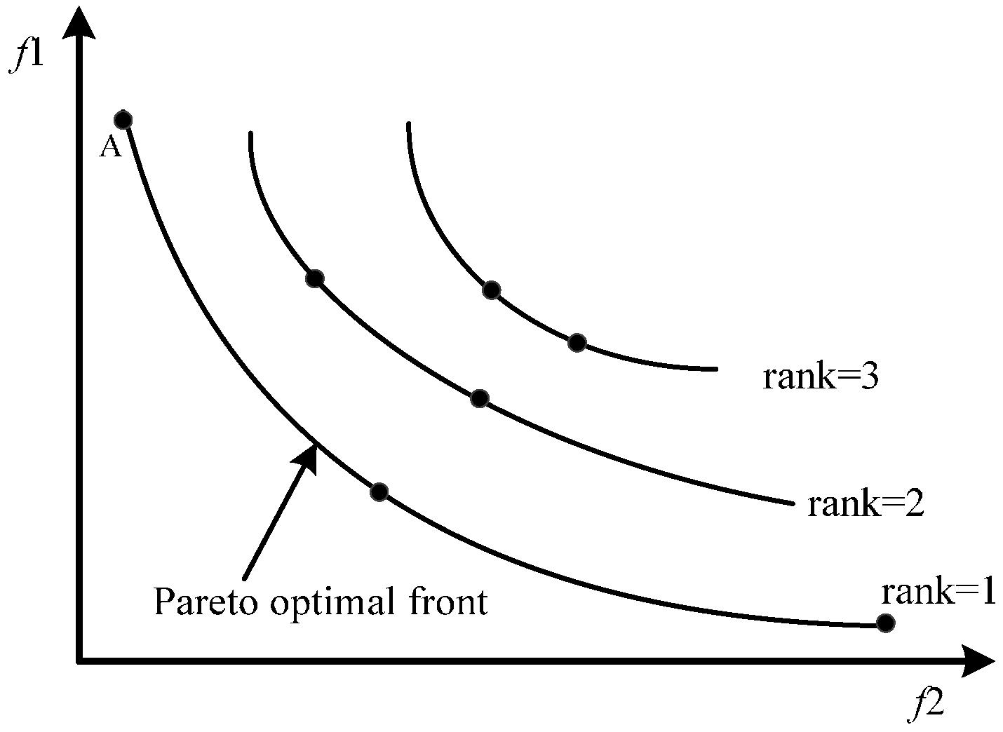
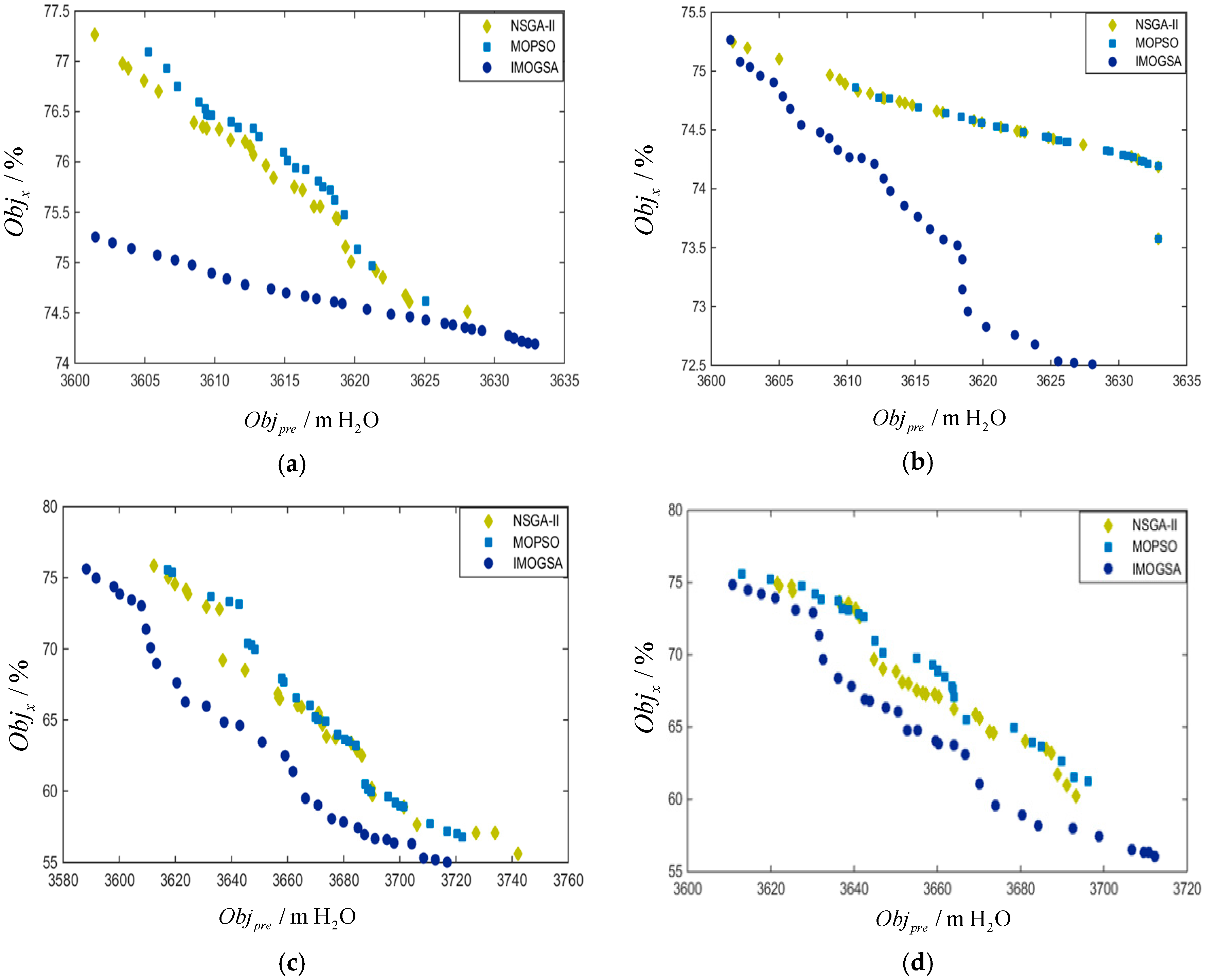
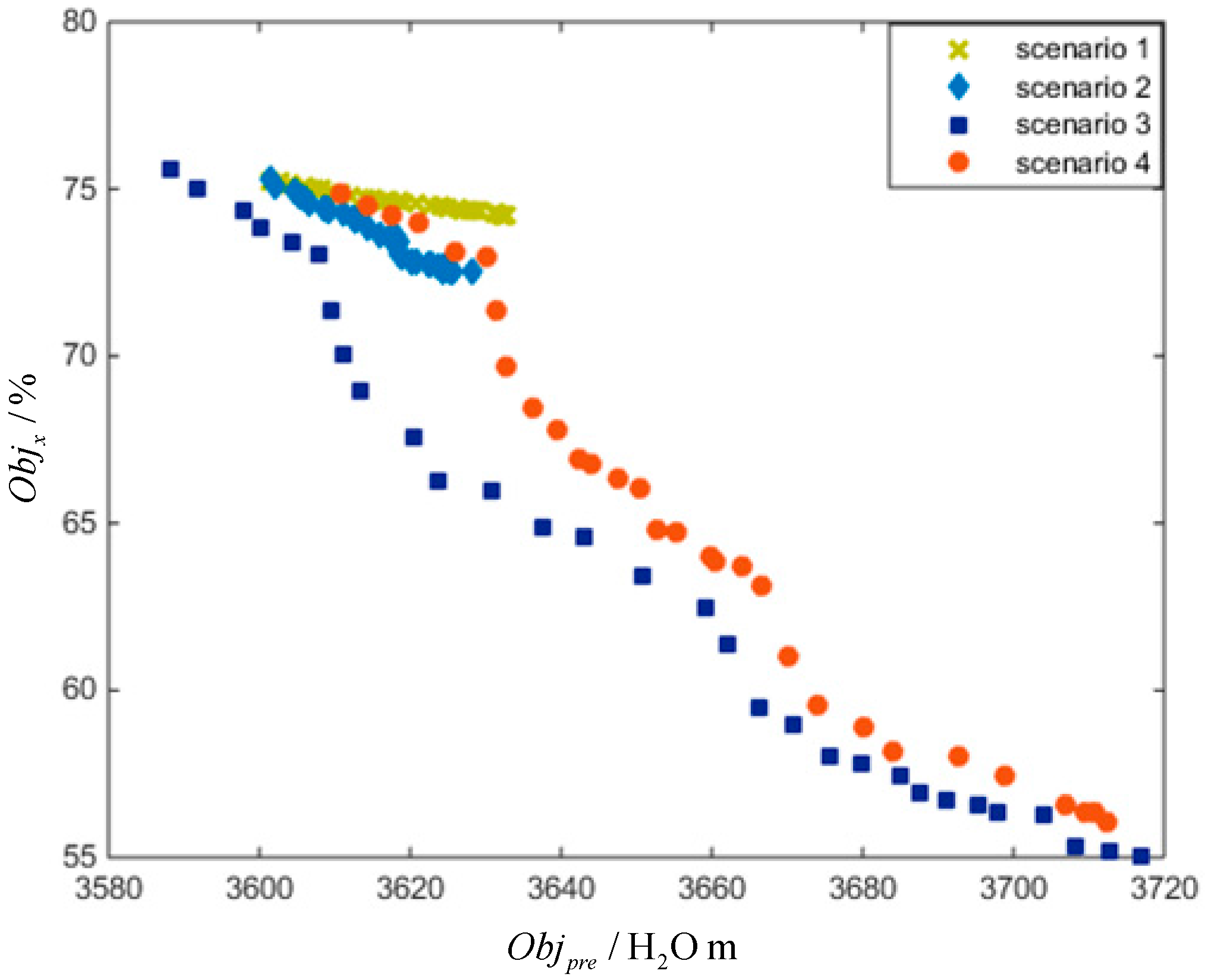
In this paper, an EMOBCGSA method is proposed to solve the OGVCS problem considering the various hydraulic and mechanical constraints. The significant innovations of the proposed method are mainly focused on the following three aspects: (1) based on a numerical calculation model of the PSHU system, a multi-objective optimization model is established, which includes hydraulic and mechanical multiple factors; (2) to improve the convergence speed and ergodicity of the algorithm, the novel population reconstruction strategy, multi-objective adaptive chemotaxis operation and velocity update method, and EAS update and maintenance strategy is introduced to improve the standard BCGSA; (3) heuristic constraint-handling strategy with elimination and local search based on violation ranking is proposed to handle the various constraints of OGVCS problems instead of the traditional penalty function, which can improve the computing efficiency. Finally, to verify the feasibility and effectiveness of the proposed EMOBCGSA method, the ‘single tube-double unit’-type PSHU system model based on actual parameters of one PSP is established and Pareto non-inferior solutions under load rejection and pump outage conditiona in different scenarios are obtained. The comparison and analysis of the optimization results achieved by EMOBCGSA and othes algorithms indicate that the proposed method can obtain better schemes with better Obj_pre and Obj_x, and the Pareto optimal solutions of EMOBCGSA possess a preferable quality and better distribution.

References

1. Yang, H.; Wei, Z.; Lou, C. Optimal design and techno-economic analysis of a hybrid solar–wind power generation system. Appl. Energy 2009, 86, 163–169. [Google Scholar] [CrossRef]
2. Zhong, Y.H.; Lu, P.; Cao, C.; Jin, B.; Jiang, H. China’s advances in new energy technology and advice on future development. Sino-Glob. Energy 2011, 16, 27–32. [Google Scholar]
3. Anagnostopoulos, J.S.; Papantonis, D.E. Pumping station design for a pumped-storage wind-hydro power plant. Energy Convers. Manag. 2007, 48, 3009–3017. [Google Scholar] [CrossRef]
4. Ding, H.; Hu, Z.; Song, Y. Stochastic optimization of the daily operation of wind farm and pumped-hydro-storage plant. Renew. Energy 2012, 48, 571–578. [Google Scholar] [CrossRef]
5. Petrakopoulou, F.; Robinson, A.; Loizidou, M. Simulation and analysis of a stand-alone solar-wind and pumped-storage hydropower plant. Energy 2016, 96, 676–683. [Google Scholar] [CrossRef]
6. Kazempour, S.J.; Moghaddam, M.P.; Haghifam, M.R.; Yousefi, G.R. Risk-constrained dynamic self-scheduling of a pumped-storage plant in the energy and ancillary service markets. Energy Convers. Manag. 2009, 50, 1368–1375. [Google Scholar] [CrossRef]
7. De Marchis, M.; Milici, B.; Volpe, R.; Messineo, A. Energy saving in water distribution network through pump as turbine generators: Economic and environmental analysis. Energies 2016, 9, 877. [Google Scholar] [CrossRef]
8. Pavesi, G.; Cavazzini, G.; Ardizzon, G. Numerical analysis of the transient behaviour of a variable speed pump-turbine during a pumping power reduction scenario. Energies 2016, 9, 534. [Google Scholar] [CrossRef]
9. Wang, Z.; Zhu, B.; Wang, X.; Qin, D. Pressure fluctuations in the s-shaped region of a reversible pump-turbine. Energies 2017, 10, 96. [Google Scholar] [CrossRef]
10. Zeng, W.; Yang, J.D.; Hu, J.H.; Yang, J.B. Guide-vane closing schemes for pump-turbines based on transient characteristics in s-shaped region. J. Fluids Eng. 2016, 138, 051302. [Google Scholar] [CrossRef]
11. Azoury, P.H.; Baasiri, M.; Najm, H. Effect of valve-closure schedule on water hammer. J. Hydraul. Eng. 1986, 112, 890–903. [Google Scholar] [CrossRef]
12. Kuwabara, T.; Katayama, K.; Nakagawa, H.; Hagiwara, H. Improvements of transient performance of pump turbine upon load rejection. In Proceedings of the Power Engineering Society Summer Meeting, Seattle, WA, USA, 16–20 July 2000; pp. 1783–1788. [Google Scholar]
13. Yu, X.; Zhang, J.; Miao, D. Innovative closure law for pump-turbines and field test verification. J. Hydraul. Eng. 2015, 141, 05014010. [Google Scholar] [CrossRef]
14. Zhang, J.; Hu, J.; Hu, M.; Fang, J.; Chen, N. Study on the reversible pump-turbine closing law and field test. In Proceedings of the ASME 2006 2nd Joint US-European Fluids Engineering Summer Meeting Collocated with the 14th International Conference on Nuclear Engineering, Miami, FL, USA, 17–20 July 2006; pp. 931–936. [Google Scholar]
15. Liu, J.T.; Liu, S.H.; Sun, Y.K.; Wu, Y.L.; Wang, L.Q. Numerical Simulation of Pressure Fluctuation of a Pump-Turbine with MGV at No-Load Condition; IOP Publishing: Beijing, China, 2012; Volume 15. [Google Scholar]
16. Pannatier, Y.; Kawkabani, B.; Nicolet, C.; Simond, J.J.; Schwery, A.; Allenbach, P. Investigation of control strategies for variable-speed pump-turbine units by using a simplified model of the converters. IEEE Trans. Ind. Electron. 2010, 53, 3039–3049. [Google Scholar] [CrossRef]
17. Sun, H.; Xiao, R.; Liu, W.; Wang, F. Analysis of S characteristics and pressure pulsations in a pump-turbine with misaligned guide vanes. J. Fluids Eng. 2013, 135, 511011. [Google Scholar] [CrossRef] [PubMed]
18. Clarke, J., Jr.; McLeskey, J.T. Multi-objective particle swarm optimization of binary geothermal power plants. Appl. Energy 2015, 138, 302–314. [Google Scholar] [CrossRef]
19. Wang, H.G.; Liang, M.A. Multi-objective particle swarm optimization. Comput. Eng. Appl. 2008, 45, 82–85. [Google Scholar]
20. Deb, K.; Pratap, A.; Agarwal, S.; Meyarivan, T. A fast and elitist multiobjective genetic algorithm: NSGA-II. IEEE Trans. Evolut. Comput. 2002, 6, 182–197. [Google Scholar] [CrossRef]
21. Basu, M. Economic environmental dispatch using multi-objective differential evolution. Appl. Soft Comput. J. 2011, 11, 2845–2853. [Google Scholar] [CrossRef]
22. Lu, Y.; Zhou, J.; Hui, Q.; Ying, W.; Zhang, Y. Environmental/economic dispatch problem of power system by using an enhanced multi-objective differential evolution algorithm. Energy Convers. Manag. 2011, 52, 1175–1183. [Google Scholar] [CrossRef]
23. Li, C.; Zhou, J.; Peng, L.; Wang, C. Short-term economic environmental hydrothermal scheduling using improved multi-objective gravitational search algorithm. Energy Convers. Manag. 2015, 89, 127–136. [Google Scholar] [CrossRef]
24. Ajami, A.; Armaghan, M. Application of multi-objective gravitational search algorithm (GSA) for power system stability enhancement by means of STATCOM. Int. Rev. Electr. Eng. 2012, 7, 4954–4962. [Google Scholar]
25. Zhou, J.; Lu, P.; Li, Y.; Wang, C.; Yuan, L.; Mo, L. Short-term hydro-thermal-wind complementary scheduling considering uncertainty of wind power using an enhanced multi-objective bee colony optimization algorithm. Energy Convers. Manag. 2016, 123, 116–129. [Google Scholar] [CrossRef]
26. Low, H.M.Y.; Chandramohan, M.; Choo, C.S. Application of multi-objective bee colony optimization algorithm to automated red teaming. In Proceedings of the 2009 Winter Simulation Conference, Austin, TX, USA, 13–16 December 2009; Volume 2, pp. 1798–1808. [Google Scholar]
27. Xu, Y.; Zhou, J.; Xue, X.; Fu, W.; Zhu, W.; Li, C. An adaptively fast fuzzy fractional order PID control for pumped storage hydro unit using improved gravitational search algorithm. Energy Convers. Manag. 2016, 111, 67–78. [Google Scholar] [CrossRef]
28. Wiggert, D.C.; Tijsseling, A.S. Fluid transients and fluid-structure interaction in flexible liquid-filled piping. Appl. Mech. Rev. 2001, 54, 455–481. [Google Scholar] [CrossRef]
29. Kung, C.; Yang, X. Energy interpretation of hydraulic transients in power plant with surge tank. J. Hydraul. Res. 1993, 31, 825–840. [Google Scholar] [CrossRef]
30. Vournas, C.D.; Papaioannou, G. Modelling and stability of a hydro plant with two surge tanks. IEEE Trans. Energy Convers. 1995, 10, 368–375. [Google Scholar] [CrossRef]
31. Zeng, Y.; Guo, Y.; Zhang, L.; Xu, T.; Dong, H. Nonlinear hydro turbine model having a surge tank. Math. Comput. Model. Dyn. Syst. 2012, 19, 12–28. [Google Scholar] [CrossRef]
32. Li, C.; Zhou, J. Parameters identification of hydraulic turbine governing system using improved gravitational search algorithm. Energy Convers. Manag. 2011, 52, 374–381. [Google Scholar] [CrossRef]
33. Xu, Y.; Zhou, J.; Zhang, Y.; Fu, W.; Zheng, Y.; Zhang, X. Parameter optimization of robust non-fragile fractional order PID controller for pump turbine governing system. In Proceedings of the 2016 Sixth International Conference on Instrumentation and Measurement, Computer, Communication and Control (IMCCC), Harbin, China, 21–23 July 2016; pp. 15–18. [Google Scholar]
34. Chen, Z.; Yuan, X.; Ji, B.; Wang, P.; Tian, H. Design of a fractional order PID controller for hydraulic turbine regulating system using chaotic non-dominated sorting genetic algorithm II. Energy Convers. Manag. 2014, 84, 390–404. [Google Scholar] [CrossRef]
35. Eberhart, R.C.; Shi, Y. Particle swarm optimization: Developments, applications and resources. In Proceedings of the 2001 Congress on Evolutionary Computation, Seoul, Korea, 27–30 May 2001; Volume 1, pp. 81–86. [Google Scholar]
36. Chen, Z.H.; Yuan, X.H.; Tian, H.; Ji, B. Improved gravitational search algorithm for parameter identification of water turbine regulation system. Energy Convers. Manag. 2014, 78, 306–315. [Google Scholar] [CrossRef]
37. Passino, K.M. Biomimicry of bacterial foraging for distributed optimization and control. IEEE Control Syst. 2002, 22, 52–67. [Google Scholar] [CrossRef]
38. Deb, K.; Mohan, M.; Mishra, S. Evaluating the ε-domination based multi-objective evolutionary algorithm for a quick computation of pareto-optimal solutions. Evolut. Comput. 2005, 13, 501–525. [Google Scholar] [CrossRef] [PubMed]
39. Kalyanmoy, D.; Manikanth, M.; Shikhar, M. Towards a quick computation of well-spread pareto-optimal solutions. In Proceedings of the 2nd International Conference on Evolutionary Multi-Criterion Optimization, Faro, Portugal, 2–11 April 2003; pp. 222–236. [Google Scholar]
40. Lim, W.J.; Jambek, A.B.; Neoh, S.C. Kursawe and ZDT functions optimization using hybrid micro genetic algorithm (HMGA). Soft Comput. 2015, 19, 3571–3580. [Google Scholar] [CrossRef]
Figure 1. Structure of a ‘single tube-double unit’-type pumped storage hydro unit system.
Energies 10 00911 g001
Figure 2. x-t characteristic line difference mesh.
Energies 10 00911 g002
Figure 3. Schematic diagram of the impedance surge tank.
Energies 10 00911 g003
Figure 4. The characteristic pump-turbine curves.
Energies 10 00911 g004
Figure 5. The layering schematic of population.
Energies 10 00911 g005
Figure 6. Schematic diagram of the straight line closure and the broken line closure.
Energies 10 00911 g006
Figure 7. The flowchart of EMOBCGSA for solving OGVCS problem.
Energies 10 00911 g007
Figure 8. The Pareto front obtained by different algorithms: (a) scenario 1; (b) scenario 2; (c) scenario 3; and (d) scenario 4.
Energies 10 00911 g008
Figure 9. The Pareto front obtained by different scenarios under load rejection.
Energies 10 00911 g009
Figure 10. The transient process of minimum Objx and Objpre schemes of scenario 3: (a) guide vane closing laws; (b) rotational speed; (c) volute end pressure; (d) draft tube inlet pressure; (e) upper surge water level and (f) down surge water level.
Energies 10 00911 g010
Figure 11. The Pareto front obtained of EMOBCGSA by different scenarios under pump outage conditions.
Energies 10 00911 g011
Figure 12. The transient process of 15 schemes by different scenarios: (a) guide vane closing laws; (b) rotational speed; (c) volute end pressure and (d) draft tube inlet pressure.
Energies 10 00911 g012