Review of PV Generator as an Input Source for Power Electronic Converters


1
Laboratory of Electrical Energy Engineering, Tampere University of Technology, Tampere 33720, Finland
2
Department of Electrical and Computer Engineering, Ben-Gurion University of the Negev, Beer-Sheva 84105, Israel
*
Author to whom correspondence should be addressed.
Energies 2017, 10(8), 1076; https://doi.org/10.3390/en10081076
Submission received: 26 June 2017
/
Revised: 17 July 2017
/
Accepted: 20 July 2017
/
Published: 25 July 2017
Abstract
:Voltage-type sources have dominated as an input source for power electronics converters for a long type. The existence of duality implies that there are also current-type sources. The growing application of renewable energy sources such as wind and solar energy has evidently shown that the current-type input sources exist in reality such as photovoltaic (PV) generator or the feedback technique used in controlling the power electronics converters in the renewable energy systems changes the power electronic converters to behaving as such. The recent research on renewable energy systems has indicated that the current-type input sources are very challenging input sources affecting the dynamics of the interfacing converters profoundly. This paper provides a comprehensive survey of the effects of the PV generator on the dynamic behavior of the corresponding interfacing power electronic converters.
1. Introduction
Voltage-type sources such as a storage battery, AC grid, and an output-voltage regulated converter have dominated as input sources for power electronic converters leading to development of multitude power-stage topologies dedicated for the above named applications [1,2]. The awareness on the depletion of fossil fuel reserves and the observed climate changes have accelerated the utilization of renewable energy sources such as wind and solar energy [3,4]. The effective utilization of these energy sources requires the use of grid-connected power electronics converters [5,6]. According to the recent knowledge [7,8,9,10], the power electronics converters applied in the renewable energy systems are usually current-fed converters because of the current-source properties of the photovoltaic (PV) generator [11,12,13,14,15] or the input-side feedback control of the renewable-energy-source-interfacing converters changing them to be current sources at their output [6,10]. In addition, it is well known that the superconducting magnetic energy storage (SMES) system, where a very large inductor serves as the energy storing element, is a perfect current source as well [16,17]. Even if the properties of the PV generator are well known, it is usually still considered to be a voltage source, when analyzing the dynamics of the converters connected to it (e.g., [18,19]) or when designing the converter power stages [20]. The substitution is usually justified by means of Norton/Thevenin transformation (e.g., [21]). The dual nature of the PV generator (i.e., the constant-current region (CCR) at the voltage less than the maximum-power-point (MPP) voltage, and the constant-voltage region (CVR) at the voltages higher than the MPP voltage) [12] may imply that the PV generator can be considered as either current or voltage source as well.
In the future, the renewable energy systems have to be able to operate both in grid-feeding (also known as grid-following, grid-parallel) and grid-forming modes [22,23,24]. In grid-forming mode, the renewable energy system delivers into the grid the maximum available energy in the renewable energy source (i.e., MPP operation) [6] or the allowed maximum power (i.e., constant-power or power-curtailment operation) [25,26,27]. The input-terminal output variables serve as the outmost feedback-loop variables of the associated power electronic converters [6]. In this operation mode, the power electronic converters can operate at all the operating points of the PV generator, when the input voltage serves as the feedback variable [28]. If the input-terminal current serves as the feedback variable, then the operating point is limited to the CVR due to the violation of Kirchhoff’s current law in CCR [29,30]. Multitude algorithms exist for locating the MPP [31,32,33,34,35,36,37,38,39,40,41] of which the perturb-and-observe [38] and the incremental-conductance methods [39,40] are most popular. In practice, both of the methods utilize the same fact that the derivative of PV power in respect to PV voltage or current equals zero at any MPP [41]. In grid-forming mode, the grid-load demand determines the output power of the renewable energy system. The output-terminal variables form the outmost feedback-loop variables of the power electronic converters [23]. Hence, the input-terminal impedance will exhibit negative incremental resistance behavior at least at the frequencies where the output-variable loop gain is high [42], which will usually limit the operating point of the PV generator in the CVR or CCR for ensuring stable operation [43,44,45,46]. The stable region depends on the design of converter-switch-control scheme or the arrangement of the feedback-controller reference and feedback signals [44].
The PV generator is a highly nonlinear input source with two distinct source regions as discussed above. Its low-frequency dynamic output impedance (i.e., incremental resistance) behaves as is characteristic to the named sources as well. At the MPPs, the PV-generator dynamic (i.e., ) and static (i.e., ) resistances are equal [47]. The dynamic changes in the PV-generator-interfacing converter are caused by the operating-point-dependent dynamic resistance, which is very high in CCR, equal to static resistance at MPP, and rather small in CVR. The typical dynamic changes are the appearance of extra right-half-plane (RHP) zero in the output control dynamics, when the converter operates in CCR [9,48,49,50], change of damping in resonant circuit along the changes in the operating point [51], and the change of sign of the control-to-output transfer function, when the operating point travels through the MPP [48,52]. In some cases, the RHP zero can be removed by the design of the converter power stage as explained in [53], but usually the RHP zero will effectively limit the output-side feedback-loop control bandwidth to rather low frequencies [42].
The main goal of the paper is to summarize the knowledge on the PV-generator behavior and its effects on the dynamics of the associated interfacing converters in order that the readers can avoid the known problems in designing the interfacing converters and the related energy systems for PV applications.
The rest of the paper is organized as follows. An introduction to the properties of PV generator affecting the interfacing converters is presented in Section 2. An introduction to the implementation of the current-fed converters and their basic dynamic properties are presented briefly in Section 3. The PV-generator-induced effects on the interfacing-converter dynamics are introduced in Section 4. The PV-generator stability issues are discussed in Section 5. The conclusions are finally drawn in Section 6.
2. PV Generator Properties
The operation of solar cell is based on the phenomenon known as PV effect, where the photons with sufficient energy emitted by the Sun will create electron-hole pairs in a proper semiconductor material, and thus electric current will flow, when the circuit is closed [54,55]. The spectral content of the Sun light at the Earth’s surface contains also a diffused (indirect) component in addition with the direct component coming from the Sun. The diffused component is created by scattering and reflections in the atmosphere and surrounding landscape and can account up to 20% of the total light incident on solar cell [55]. The nominal value of the direct and diffused irradiations at the Earth’s surface is considered to be 1 kW/m2 but it is naturally varying depending on the atmospheric conditions and the angle of incident of the irradiation over the location of the cell (cf. Figure 1a). In certain conditions during a half-cloudy day, the maximum irradiance can exceed 1 kW/m2 due to the phenomenon known as cloud enhancement [56] (cf. Figure 1b). It is obvious that the cloud enhancement has to be taken into account, when designing the PV-interfacing-converter power stages as well [57].
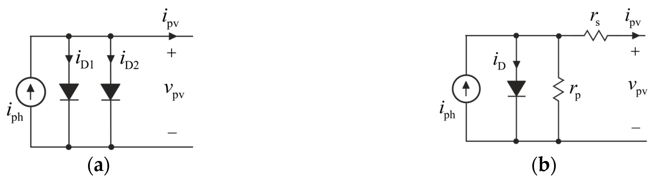
In principle, a solar cell can be represented by an equivalent circuit composing of a current source in parallel with two diodes as depicted in Figure 2a [11,55]. The ideal current-voltage (I-V) characteristics of a cell can be given by:
where (i.e., the electron charge), (i.e., the Boltzmann constant), denotes the temperature in Kelvin degrees, and and denote the saturation current of the diodes. The two-diode equivalent circuit is most often simplified to a single diode model (cf. Figure 2b), where the contributions of the two diodes are combined as follows [12,13,14,15,55]:
where denotes the combined diode saturation current and the diode ideality factor. The single-diode model yields accurate results, when the irradiance level is sufficiently high, but it loses its accuracy at lower irradiance levels such as during a cloudy day, when the irradiance is at most 20% of clear-sky conditions [59]. Many of the developed solar-cell models are claimed to be comprehensive as in [13,15] but the models do not include the solar-cell capacitance [60,61,62], which would be necessary for studying the effect of connection-cable-induced resonance on the interfacing converter or other similar adverse effects. Due to the existence of PN-diode structure in the solar cell, it is obvious that the cell capacitance is highest in the open-circuit condition, where all the photocurrent is flowing through the diodes. The PN-diode structure implies also that the open-circuit voltage is dependent on the cell temperature, and it will decrease along the increase in the cell temperature due to the negative temperature coefficient of PN diode [63].
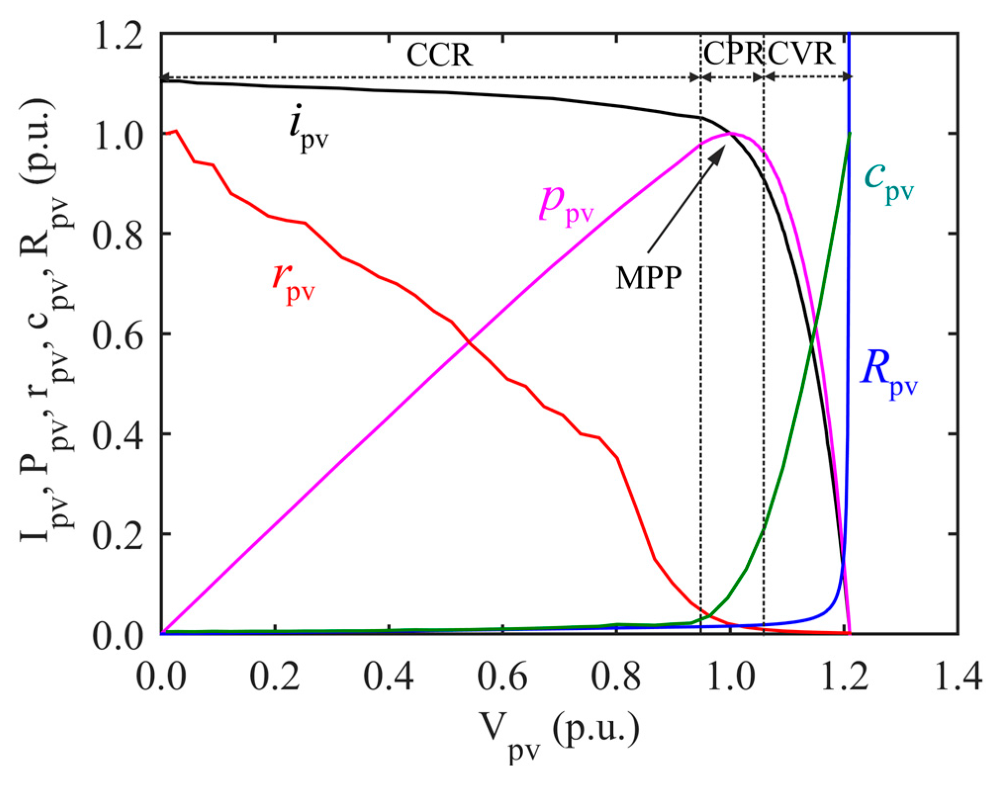
Figure 3 shows the characteristic per-unit curves of a Raloss SR30-36 solar panel (Shanghai Raloss Energy Technology, Co., Ltd, Shanghai, China) illuminated by an artificial light source capable of producing irradiation of 500 W/m2 shown in Figure 4. The panel is specified more in detail in [28]. In Figure 3, the authentic PV current and voltage values are divided by their corresponding MPP values (0.91 A and 16 V), the dynamic and static resistance values are divided by the maximum value of dynamic resistance (), and the dynamic capacitor values are dived by the corresponding maximum value of .
The measurement of the PV-panel steady-state characteristics is performed by connecting a voltage-type electronic source at the output terminal of the PV panel for changing the operating point from the short-circuit condition to open-circuit condition. The frequency response of the PV panel output impedance is measured at every operating point by means of a frequency-response analyzer by injecting a proper excitation signal at the PV panel voltage. The dynamic resistance and capacitance values are extracted from the measured frequency responses based on Equation (3).
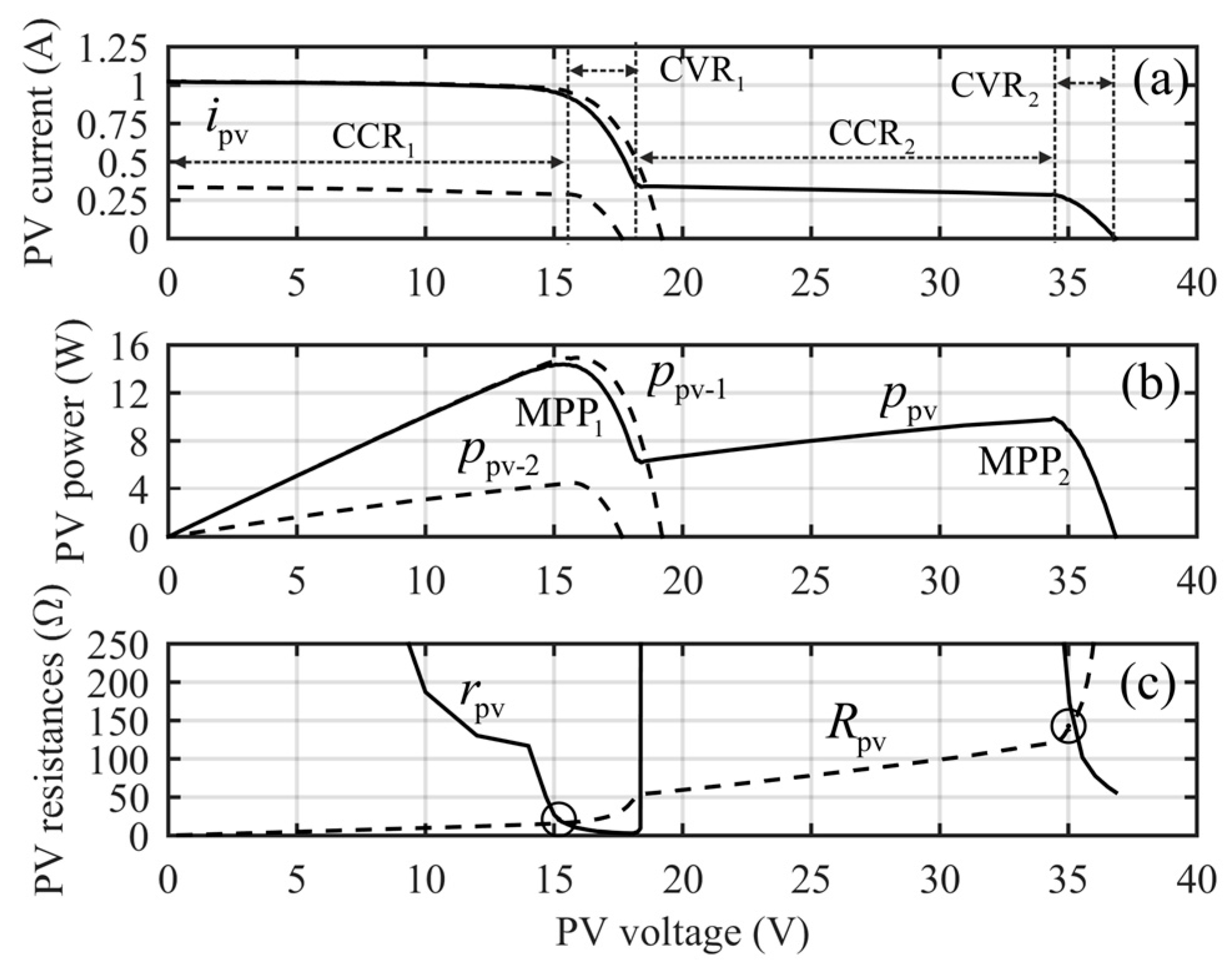
As discussed earlier, the operating points of PV generator is typically divided into two distinct regions (i.e., CCR and CVR), which are separated by the MPP voltage as depicted in Figure 3. In Ref. [64], two different power regions are added in vicinity of MPP, which are justified due to the behavior of the dynamic resistance within those regions. The region around the MPP is denoted as constant-power region (CPR) (cf. Figure 3) in Refs. [51,65,66], because the change in PV power is actually very small within CPR as shown in Figure 5. The same phenomenon is also utilized in tracking the MPP as presented for example in [36,37], which justifies well the existence of CPR. The existence of CPR affects only the MPP-tracking process in such a manner that the exact MPP is difficult to be located due to the finite resolution of the current and voltage measurements [51]. Therefore, the algorithm can locate the MPP at any of the operating points within the CPR [51].
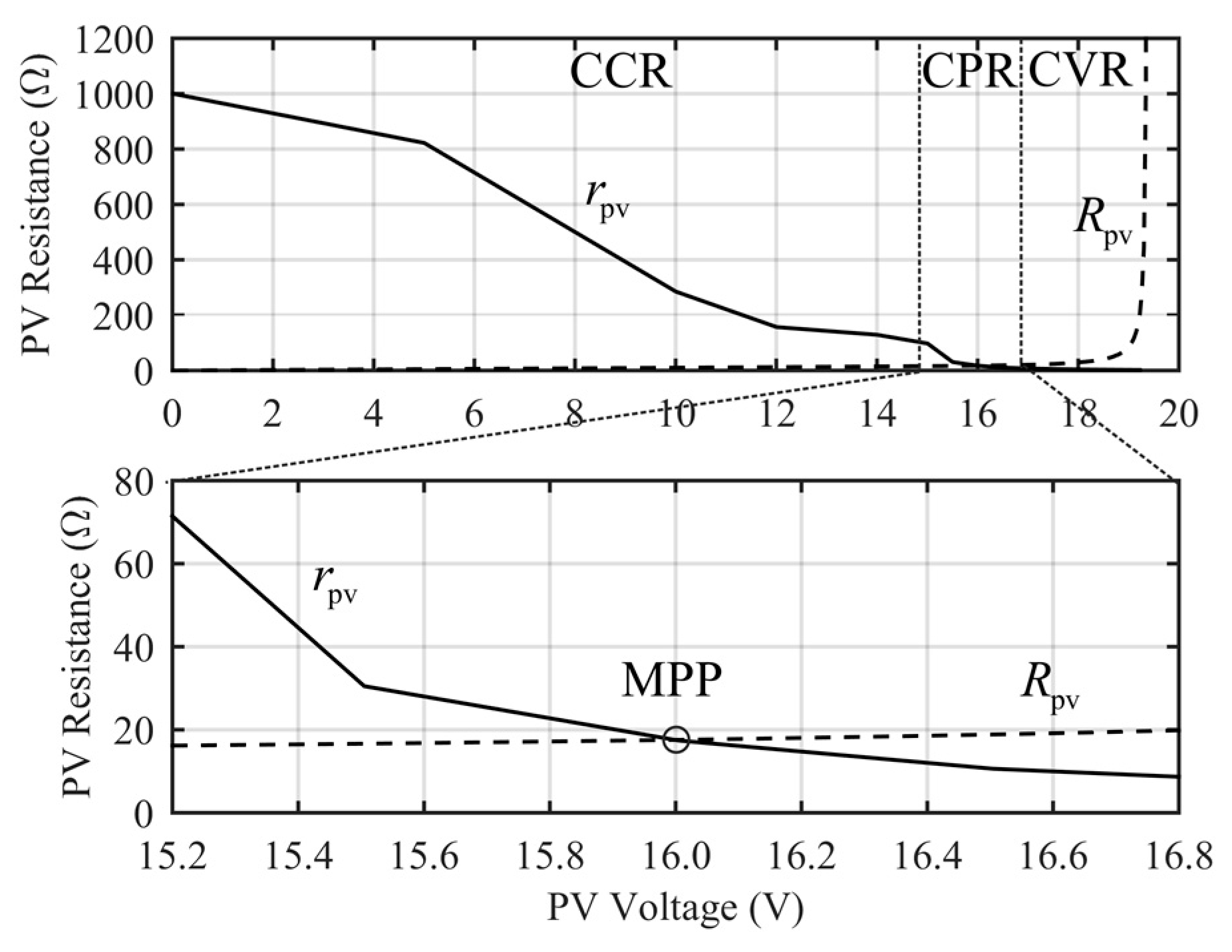
Figure 6 shows the measured dynamic and static resistances of the Raloss SR30-36 PV panel and their behavior in CPR. As the bottom subfigure shows, the exact location of the MPP is defined by the equality [47]. It is usually assumed that the incremental-conductance-based MPP tracking method is fast and accurate due to utilizing the named equality [39,40], but the same measurement accuracy problems as discussed above will also affect it (cf. Figure 6; the behavior of ) [41].
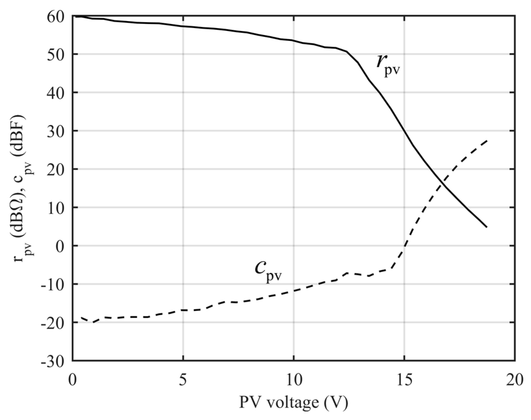
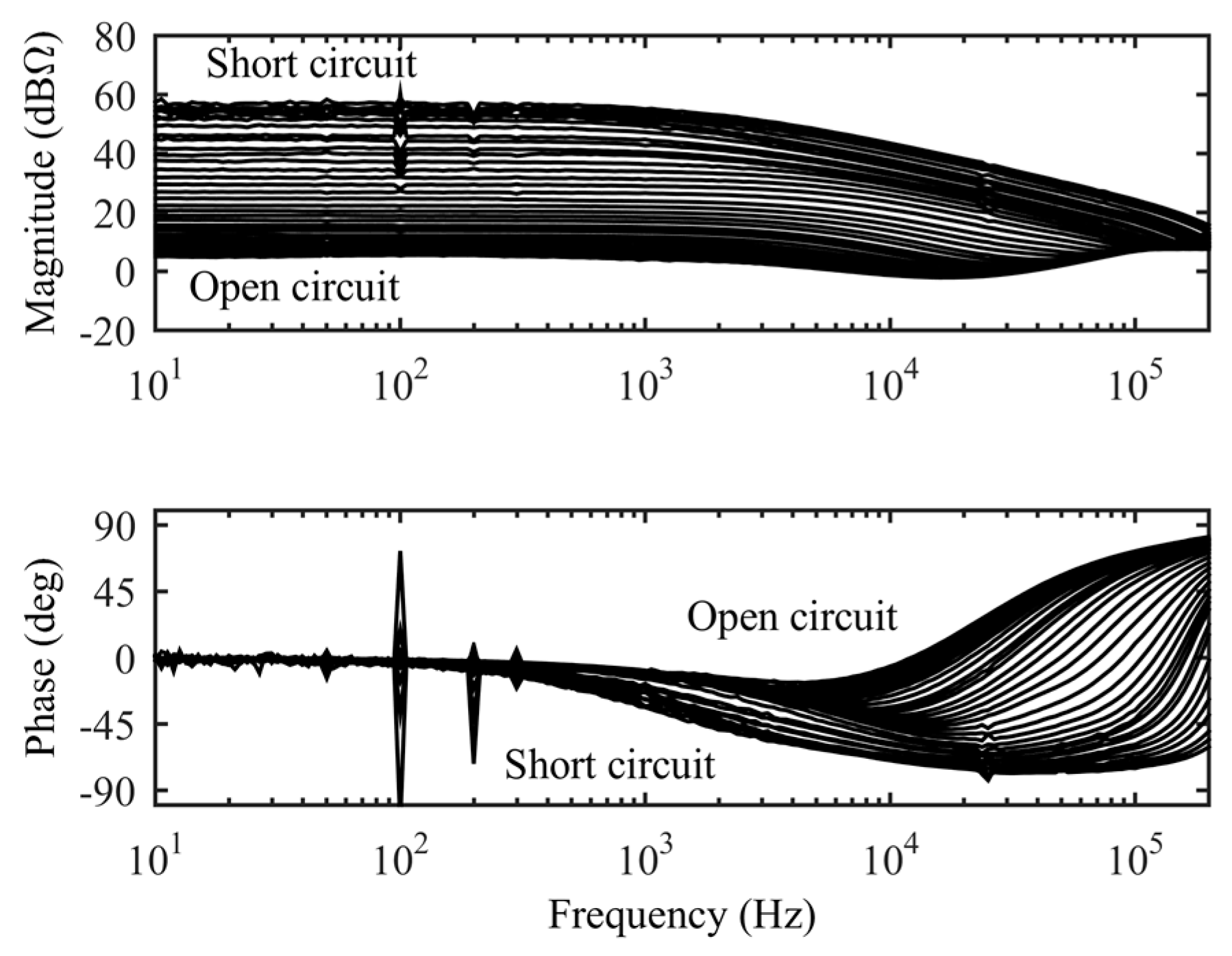
Figure 7 shows the measured dynamic resistance () and capacitance () values expressed as dB values. Both curves show (i.e., two different slopes) that the accurate solar-cell model comprises two different diodes, as the semiconductor theory predicts [55].
Figure 8 shows the measured output impedance of the Raloss SR30-36 PV panel, when the operating point is varied from short-circuit to open-circuit condition. The RC-circuit-like behavior governs the output-impedance behavior up to 10 kHz. At higher frequencies, the connection-cable inductance starts dominating the behavior. Therefore, the solar cell output impedance can be given by:
where and are as denoted in Figure 2b, and and denote the PN-diode dynamic resistance and capacitance, respectively. The low-frequency part of the output impedance is usually denoted by , which equals . A practical PV generator composes of a number of series connected cells as a PV panel. The PV panels are usually further connected in series as a PV string, etc. Therefore, the final structure of the PV generator affects the value of as well. The dynamic resistance was commonly considered a negative incremental resistance (e.g., [64,66]), but Figure 8 shows definitively that is a positive resistance.
A PV panel is usually constructed by using three PV modules in series, and a shunt diode is connected across each module [67,68]. The goal of the shunt diodes is to protect the solar cells from overheating in the case of non-uniform irradiation over the surface of the panel [67]. As the solar cells are constant-current sources and their photocurrent corresponds directly to the level of irradiation [55], the non-uniform irradiation level will force the cell currents to be different as well. The highest module current will determine the overall panel output current. Due to the series connection of the modules, the shunt diodes of the modules will form a current path for the excess current for satisfying Kirchhoff’s current law within the panel interfaces. The conduction of the shunt diodes will create excess MPPs in the PV generator [69,70,71,72] (cf. Figure 9). At each MPP, the corresponding dynamic and static resistances are equal [47] (cf. Figure 9c). In vicinity of the MPPs, CCR exists at the voltages lower than the MPP voltage and CVR exists at the voltages higher than the MPP voltage as Figure 9a clearly shows (cf. the behavior of dynamic resistance in Figure 9c). The data shown in Figure 9 are produced by connecting two Raloss SR30-36 panels in series with a shunt diode across each of them and providing non-uniform illumination condition (i.e., Panel 1 = 500 W/m2 and Panel 2 = 150 W/m2). The measured I-V and P-V curves are shown in Figure 9a,b, and the behavior of the measured dynamic and static resistances is shown in Figure 9c, respectively. Figure 9b also clearly shows that the MPP lying at the highest voltage is not necessarily the global MPP.
It is well known that the dynamic resistance () will cause the changes observed in dynamics of the PV-generator-interfacing converter [9]. The most significant dynamic changes will take place, when the PV-generator operating point travels through any of the MPPs. The dynamic issues are discussed in detail in Section 4 and Section 5.
3. Implementing Current-Fed Converters
The existence of duality in circuit theory implies also the existence of current-fed converters, where the input source is a current source [73,74]. In power electronics, the terms “current sourced” and “current fed” have been used commonly to denote the voltage-fed converters, where an inductor is placed in the current path of the input terminal [75,76,77,78,79]. This situation may cause confusion, when real current-fed converters are regularly used in renewable-energy-interfacing systems.
A current-fed converter can be implemented in three different ways: (i) by utilizing capacitive switching cells [80,81], similar to inductive switching cells being utilized to implement voltage-fed converters [1,2,81]; (ii) by applying duality principles to transform a voltage-fed converter into the corresponding current-fed converter [17,53,78,82,83,84,85]; and (iii) by adding a capacitor at the input terminal of the voltage-fed converter [86,87,88] for satisfying the interfacing constraints stipulated by the current-type input source [89,90].
The duality transformation is, in principle, based on the duality transformation pairs depicted in Figure 10 by applying either the graph method described in [74] and demonstrated in [84] or a more convenient method introduced in [82,83] and demonstrated in [53,84]. The application of the graph method in [53] failed due to a certain structure in the voltage-fed superbuck converter but it succeeded easily with the method introduced in [82]. The voltage-fed superbuck converter is the same converter as analyzed in [76] (cf. Figure 11a).
The duality-transformation method introduced in [82] is such that a dot is placed inside every mesh in the circuit and one (ground) outside the circuit as depicted in Figure 11a. All the adjacent dots are connected together with the dual of the component or structure of the circuit branch over which the connection takes place as illustrated in Figure 11a (i.e., the dashed line). The outcome of the transformation is given explicitly in Figure 11b. It is essential to change also the conduction times of the switches according to the duality transformation pairs in Figure 10 (i.e., the last row).
The duality transformation will produce a converter, which has, in principle, the same steady- state and dynamic properties as the original converter has. The ideal input-to-output gain (M(D)) will be the same for both of the converters, but, in the case of voltage-fed converter, it represents the input-to-output voltage ratio, and, in the case of current-fed converter, the input-to-output current ratio.
In general, the equality in dynamic behavior between the voltage-fed converter and its current-fed dual is valid also in the case of the buck converters in Figure 12. It is well known that the basic voltage-fed buck converter (Figure 12a) does not contain control-related anomalies even if an LC-type input filter is connected at its input terminal [42]. The current-fed buck converter in Figure 11b does not contain such anomalies [91] (cf. Equation (4)), but the converter cannot be used as such in the PV-generator interfacing because of the existence of PV-generator capacitor (cf. [62]), and therefore, an LC-type input filter has to be connected at its input terminal (cf. Figure 13). The input filter will induce the appearance of two RHP zeros into the output control dynamics, which will effectively limit the control bandwidth of the converter [42]. The control-to-output transfer functions of the current-fed buck converter without and with the input filter are given in Equations (4) and (5), respectively. Equation (5) indicates that the converter with input filter contains two RHP zeros approximately at and (cf. Figure 12 for the variable and component definitions). The RHP zeros are the same as in the output control dynamics of the current-fed boost-power-stage converter reported in [50].
The power stages of the voltage-fed converters can be used as current-fed converters by connecting a capacitor at their input terminal [10,48,64,86,87,88,89] for satisfying the interfacing constraints stipulated by the current-type input source [89,90]. This method is the most popular method. It changes the steady-state and dynamic properties of the current-fed converter to resemble the properties of the dual of the corresponding voltage-fed converter (i.e., a buck converter is the dual of boost converter and vice versa) (cf. [48,50]). If the original switch-control scheme is maintained the same as in the voltage-fed converter, then the duty ratio has to be decremented for increasing the output variables of the current-fed converter [64] or the gate-drive signals have to be inverted for increasing the output variables along the increase in duty ratio as well [87].
4. PV Generator Effect on Interfacing Converter
As discussed in [68], the PV generator can be configured as an array-based input source, a string-based input source, a panel, or submodule-based input source. The panel or submodule-based configurations are indented to reduce the energy losses due to mismatches in the irradiation conditions over the surface of the PV generator by providing MPP tracking in a more granular manner than in the PV array and string-based configurations [92]. Despite the configuration of the input source, the PV-generator effects on the dynamics of the interfacing converter are the same and dependent mainly on the feedback arrangements in the interfacing converter.
In general, the input-source effects on the converter dynamics can be computed based on Figure 14, where S denotes the input-source system, and C the converter system. The variables denoted by u are the input variables, and the variables denoted by y are the output variables. The variables denoted by v and i are the physical voltages and currents of the subsystems. The subscripts “in” and “out” denote the terminal, where the corresponding variables exist.
Based on the denotations in Figure 14, the mapping from the cascaded system input variables (i.e., and ) to the cascaded system output variables (i.e., and ) can be given by:
where denotes the transfer functions of the converter, denotes the transfer functions of the input source and the special parameters of the converter and can be given by:
The set of converter transfer functions in general form are given in Equation (8). The input source is assumed to be composed of an ideal voltage or current source with a corresponding ohmic loss element. Therefore, the transfer functions of the source system can be given as shown in Equation (9). The negative sign of the element (2,2) in Equations (8) and (9) is the consequence of the direction of the output current of the subcircuits (i.e., flowing out of the terminal).
Equation (6) shows that all the converter transfer functions () (cf. Equation (8)) are affected by the impedance-based sensitivity function , where the impedance ratio () depends on the type of the input source (i.e., in the case of voltage source, is an impedance, and, in the case of current source, is an admittance). In practice, this means that the impedance ratios are an inverse of each other, which affects fundamentally e.g., the stability analysis of the source-coupled converter system (i.e., the stability can be assessed by means of the impedance ratio, which is known as minor-loop gain [52]). The general source-effect formulation in Equation (6) is utilized to obtaining the outcomes of the interaction analyses shown in the following subsections and in the stability analyses given in Section 5. More specific information on computing source effects and on the special parameters in [7] can be found from [28,29,30,42,50,52,53].
4.1. PV Energy System Structure and Operation Modes
The solar energy system can be a single or double-stage system in terms of power-electronic-converter arrangement in the system. In a single-stage system (cf. Figure 15), the grid-connected inverter is directly connected to the PV-generator terminals. In a double-stage or cascaded system, the grid-connected inverter is connected into the PV generator through a DC-DC-converter stage. Usually the solar energy system is working in grid-feeding mode (cf. Figure 15a) delivering either maximum available power (i.e., MPP operation) in the PV generator [26] or a part of it (i.e., constant-power or power-curtailment operation) [25,27] into the grid. In this operation mode, all the outmost feedback loops are taken form the input-terminal voltage of the associated converters as depicted in Figure 15a. In this mode of operation, the PV-generator-interfacing DC-DC stage can be operated in open-loop mode as well [51]. In microgrids or in the case of islanding mode of operation, the solar energy system is required to operate also in grid-forming mode (cf. Figure 15b) to producing the grid voltage as well as its frequency [22,23,24]. In this mode, all the outmost feedback loops have to be taken from the output terminals of the associated converters as depicted in Figure 15b. Due to the feedback from the output-terminal variables, the system will be prone to instability due to the non-linear nature of the PV generator and the high-gain output-terminal feedback loops of the associated converters (i.e., negative incremental resistance of the input impedance) [43,44,45,46,86]. The stability issues related to the feedback control of the output-terminal variables are discussed more in detail in Section 5.
4.2. Dynamic Effects
As discussed in Section 2, the PV generator can be represented by a parallel connection of a constant-current source () and an admittance (), where denotes the total photocurrent of the PV generator and its output admittance (cf. Equation (3)). The diode dynamic resistance () is usually much higher than the series resistance () (cf. Figure 2b), and, therefore, . As Figure 8 indicates, the resistance dominates in () up to some kHz, and therefore, it may be obvious that the dynamic resistance () will be responsible for the observed changes in the interfacing-converter dynamics [9,10,28,50]. The input capacitor or LC input filter is, in practice, an essential part in the PV-interfacing converter either for satisfying the theoretical terminal constrains stipulated by the current source (i.e., input capacitor) [90] or for preventing the output capacitance of the PV generator to damage the associated switches (i.e., LC input filter, cf. Figure 13) [62]. Therefore, it may be obvious based on the behavior of (cf. Figure 3) that effectively controls the role of the input-capacitor voltage as a state variable in the converter dynamics (cf. Figure 16 and Figure 17): is small in CVR and, thus, it effectively dominates the behavior of the parallel impedance (i.e., the order of system is effectively reduced by one). is large in CCR, and thus the input capacitor in itself dominates the parallel impedance, and the input-capacitor voltage is fully a state variable.
The typical effects of the PV generator on the interfacing-converter open-loop dynamics are the modifying of the resonance damping behavior [51] along the changes in the PV-generator operating point (cf. Figure 16) as well as creating an RHP zero in the control-to-output transfer function, when the converter operates in CCR (cf. Figure 17) [10,28,48,49,52,85,87]. The RHP zero can be approximately given by (cf. Equation (5)). The open-loop input-control dynamics does not usually contain RHP zeros (cf. [48,50,52,53]). If the converter operates in open loop or the feedback loops are taken from the input voltage then the RHP zero does not have effect on the interfacing-converter behavior. Figure 17 shows also that the phase of the control-to-output transfer function will change by 180 degrees, when the operating point travels through the MPP. In practice, this implies that the output-terminal-feedback-controlled converter will become unstable, when the operating point travels through the MPPs.
The grid-connected inverters are most often designed with cascaded control loops in such a manner that the inverter-output-current feedback loop forms the inner loop and the DC-link-voltage feedback loop forms the outer loop, respectively [6,10]. The open-loop output-control dynamics of the inverter contain an RHP zero, when the inverter operates in CCR [10]. The closed output-current-feedback loop transforms the RHP zero into an RHP pole in the control-to-input-voltage transfer function (i.e., the inverter is unstable in open loop) [10,93,94]. For ensuring stable inverter operation, the control bandwidth of the input-voltage-feedback loop has to be sufficiently higher than the frequency of the RHP pole [10,42]. In practice, the crossover frequency of the dc-link feedback loop has to be sufficiently less than twice the grid frequency in order to avoid to injecting corresponding harmonic current into the grid. Therefore, the stability requires to using a dc-link capacitor with sufficient capacitance as discussed explicitly in [10].
The associated pole can be approximated, in general, according to Equation (10), where denotes the input terminal capacitor of the inverter, and denote the input current and voltage of the inverter, and the low-frequency output admittance of the input source of the inverter [10,93,94,95,96].
In single-stage systems, where the inverter is connected directly to the PV-generator terminal, the pole (zero) in Equation (10) can be given by:
According to the behavior of and (cf. Figure 3), the pole in (11) lies in RHP in CCR, and it can be given by (i.e., ) . When the operating point moves into CVR, the pole moves into the left-half plane (LHP) of complex plane, and it can be given by (i.e., ) (Note: The negative sign of (11) in CVR indicates LHP pole (zero)).
In cascaded systems, the inverter is connected via the DC-DC stage into the terminals of the PV generator. Therefore, and denote the dc-link current () and voltage (), and denotes the low-frequency output impedance of the DC-DC converter stage. As stated earlier, the DC-DC stage can be operated either in open or closed-loop mode [51,65]. In open-loop mode, the PV-generator-affected open-loop output admittance () can be approximated [95] by , when is usually much higher than the ohmic losses in the interfacing DC-DC stage. In addition, the dc-link voltage and current ratio (i.e., dc-link static resistance) can be given as the function of the PV-generator static resistance by [94]. Consequently, Equation (10) can be given by Equation (12) from which the RHP pole can be computed to be (i.e., ) and the LHP pole to be (i.e., ), respectively.
where denotes the ideal input-to-output gain of the DC-DC stage.
In closed-loop mode, [50,95] and therefore, the pole in Equation (10) will locate at origin. In practice, the losses in the associated converters may affect the pole in such a manner that it will locate in vicinity of the origin either in RHP or LHP. In practice, the inverter will be stable independent of the size of the input capacitor, because the control bandwidth of the dc-link voltage-feedback loop has to be always high enough for the proper operation of the inverter [10]. According to Equations (11) and (12), we can concluded that the pole approaches the origin, when the PV-generator operating point approaches the MPP (i.e., [47]), and therefore, the highest dc-link-voltage control bandwidth is required for the stable operation in the voltages below the MPP voltage (cf. [10]). In addition, the maximum input-capacitor (i.e., dc-link capacitor) size is required, when the inverter is connected directly to the PV-generator terminals [10].
It has been observed that the buck-power-stage converter under peak-current-mode (PCM) control can become unstable as well, when used as a PV-generator interfacing converter under input-voltage-feedback control [97,98]. The reason for the instability is the same as discussed above in the case of the cascaded-controlled inverter: The output-side control dynamics of the buck-power-stage converter contains an RHP zero [48]. The inductor-current feedback loop contains the same RHP zero, which becomes an RHP pole in the input-side control dynamics. The converter can be stabilized by designing the input-voltage control bandwidth to be sufficiently higher than the frequency of the RHP pole. Commonly, the input capacitor of the converter is quite large and therefore, the RHP pole locates at low frequencies and therefore, the input-voltage-loop control bandwidth satisfies the stability requirements easily as such. The existence of the RHP pole in [98] is cancelled by compensating heavily the inductor-current feedback, which effectively removes the effect of PCM control in the converter.
5. Stability Issues
As discussed in Section 4, the renewable energy systems have to be able to operate both in grid-feeding and grid-forming modes [23,24,99]. In grid-feeding mode [23], the system is stable at all the operating points of the PV generator, if the associated converters are properly designed as shown in Figure 18. Figure 19 shows the behavior of the PV-generator voltage and current as well as the output current of the input-current-controlled buck-type interfacing converter. The figure shows explicitly that the input-current-controlled interfacing converter can operate in a stable manner only in the CVR of the PV generator. As stated earlier, the reason for the phenomenon is the violation of Kirchhoff’s current law, when the converter enters into the CCR of the PV generator.
5.1. Grid-Forming-Mode Operation
In grid-forming mode, the output-side feedback loops will cause the input impedance of the converters to contain negative-incremental-resistance behavior in the frequency range, where the magnitude of the feedback loops is high [42] (cf. Figure 20 and Figure 21). In addition, the load demand of the energy system will determine at which operating point the associated converters are working. If the load power equals or exceed the maximum available power in the PV generator then the system will be unstable, and the PV voltage will collapse [43]. The change of phase of the control-to-output transfer function in Figure 17 by 180 degrees, when the operating point travels through the MPP, implies the instability to take place as well.
It is well known that the environmental conditions over the surface of PV generator such as cloud passing will cause non-uniform irradiation condition on the surface of the PV generator, and thus fluctuations in the available power supplying capacity of the PV generator (cf. Figure 1). Refs. [100,101,102,103] provide a comprehensive analysis of the associated phenomena (i.e., the time scale of the irradiation changes, etc.) and the effect of the mitigation techniques to reduce the fluctuations by reconfiguring the PV array, etc. In addition to the power fluctuations, the non-uniform irradiation condition will usually cause multiple MPPs to appear in the PV generator (cf. Figure 9) [69,70,71,72]. The fluctuation of the available power supplying capacity of the PV generator and the appearance of multiple MPPs are detrimental, especially, in the grid-feeding mode of operation due to the grid-originated load-power demand as discussed above.
Therefore, it is obvious that the PV energy systems cannot operate reliably without the utilization of stored energy [104,105]. Although different alternatives exist for mitigating the detrimental effects of the power fluctuations [106], the most practical method is the utilization of battery-energy-storage-based devices [107,108,109,110]. As discussed above, the grid-feeding-mode systems are prone to instability [43,44,45,86] and the energy-storage devices can be used to keep the system stable in the case of detrimental power fluctuations. The stability studies on the topic (e.g., [110,111,112]) have been concentrating only on the grid-feeding mode of operation, and, therefore, there are no studies published related to the grid-forming mode according to the authors’ knowledge.
The foundation for the cascaded-system interconnection analyses, which are based on certain impedance ratios, has been laid down in [113,114] applying Nyquist stability criterion [115,116]. The analysis methods are developed further in many publications (e.g., [28,42,117,118,119,120,121,122,123,124,125,126,127]). The further developments are mainly concentrated on enlarging of the allowed area in complex plane, where the impedance ratio is allowed to lie without causing instability [117,118,122], on making the special parameters governing the interactions in the converters to be explicitly solvable [119,122], and on extending the methods into the grid-connected three-phase converters as well [123,124,125,126,127]. The interactions are caused by the source and load impedances through the different impedance ratios in the associated converters [122].
The gate-control scheme of the interfacing converter determines in which operational region the converter will be working in a stable manner. If the switch control scheme is the same as in the corresponding voltage-fed converter then the stable operation region is CVR. If the switch control scheme is designed for operation as a current-fed converter then the stable operation region is CCR, respectively. The stable operational regions can be changed by configuring the control system in such a manner that the feedback-variable and reference signals are interchanged in respect to their normal arrangement [44,45]. The reason for the determining role of the switch-control scheme is its effect on the behavior of the converter output variables, when the duty ratio is increased: The natural behavior is such that the increase in the duty ratio will also increase the output variables. In voltage and current-fed converters, the input and output variables are interchanged. Therefore, the voltage-fed-converter duty ratio has to be changed to its complement in the current-fed converter for the voltage-fed power stage to operate properly under current-type input source and vice versa. The boost-power-stage converter reported in [50] (cf. Figure 22) is utilized to produce the experimental behavior of the interfacing converter during the instability in Section 5.2 and Section 5.3 under output-voltage feedback control. In Section 5.2, the switch-control scheme of the converter corresponds to the switch-control scheme used typically in voltage-domain applications (i.e., voltage-fed power stage) [42]. In Section 5.3, the switch-control scheme is inverted (i.e., current-fed power stage).
5.2. Grid-Forming-Mode Operation: Voltage-Fed Converter
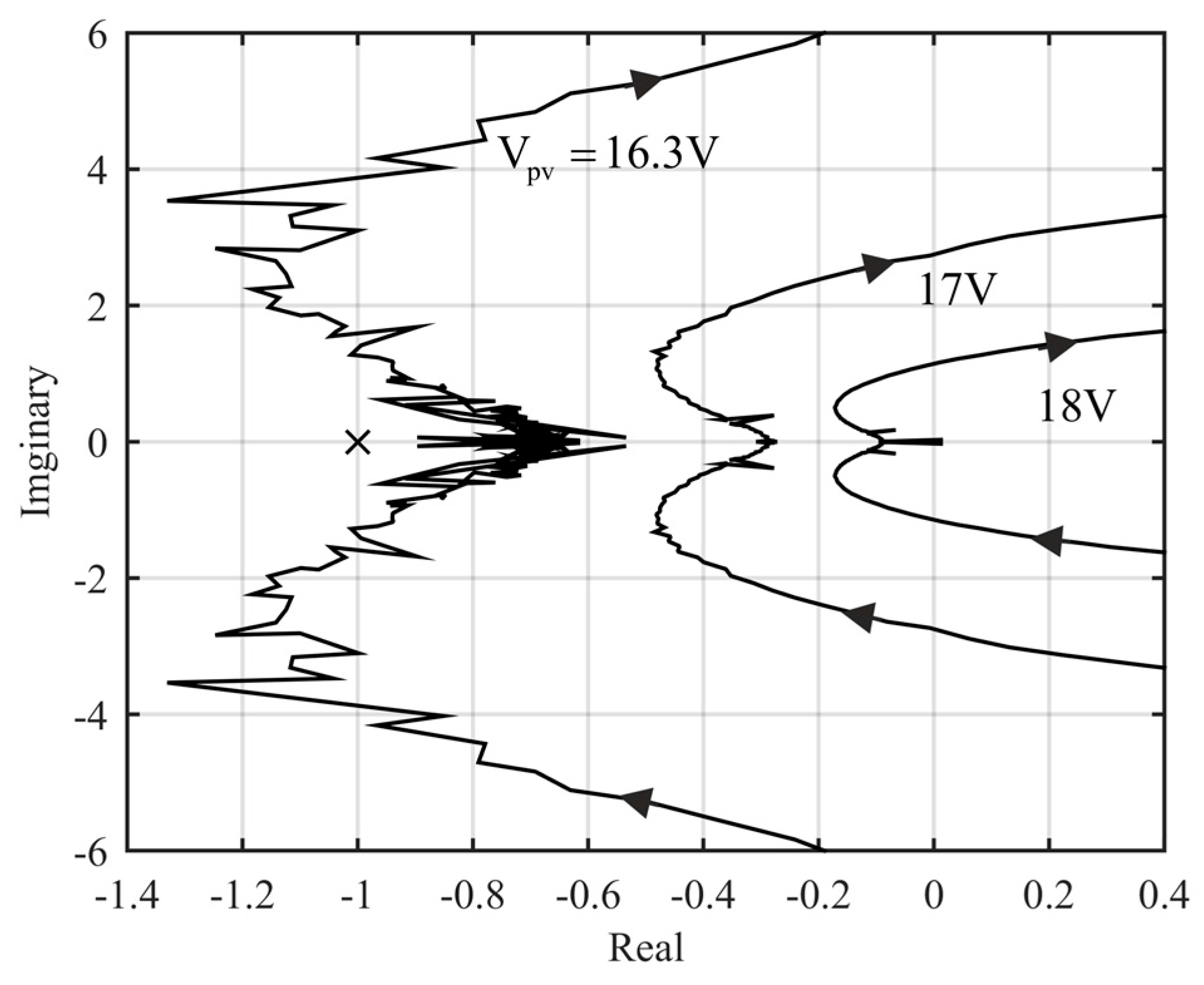
Figure 23 shows the Nyquist plot of the impedance ratio composing of the PV-generator output impedance and the closed-loop input impedance of the voltage-fed power-stage converter under output-voltage-feedback control, when the operating point approaches the MPP (16 V) in CVR. At MPP, the Nyquist plot will travel through the critical point (−1, 0), and instability takes place as shown in Figure 23. As a consequence of the instability, the PV voltage collapses to zero (cf. Figure 24) (i.e., the low-side MOSFET stays permanently on (cf. Figure 22)). Even if the load current of the converter is set to zero (cf. Figure 24, at time ), the converter does not recover from the instability. The reason for this behavior is the switch-control scheme, which forces the operating point to lie permanently in CCR as discussed in Section 5.1.
It may be obvious that the stable operational region of the output-voltage-feedback-controlled voltage-fed power-stage converter will be always in CVR starting from the open-circuit condition to the highest MPP voltage. In the case of multiple MPPs (cf. Figure 9), the highest-voltage MPP may not be the operating point, at which the highest power lies at all. This may complicate the situation further from the stability point of view. Moving the operating point to the absolute maximum power point or global MPP may not be possible without energy-storage assisted measures. The tracking of the maximum available power in the PV generator is not possible either due to the possibility of instability. The similar behavior will take place also in the PCM-controlled boost converter as reported in [46] due to the negative incremental input resistance of the converter [42].
5.3. Grid-Forming-Mode Operation: Current-Fed Converter
Figure 25 shows the Nyquist plot of the impedance ratio composing of the closed-loop input impedance of the current-fed power-stage converter under output-voltage-feedback control and the PV-generator output impedance, when the operating point approaches the MPP (16 V) in CCR. At MPP, the Nyquist plot will travel through the critical point (−1, 0), and instability takes place as shown in Figure 26. As a consequence of the instability, the low-side MOSFET of the converter (cf. Figure 22) stays permanently open and, therefore, the PV generator supplies the load current of the interfacing converter through the high-side diode (cf. Figure 22 and Figure 26). When the load current is reduced at time (cf. Figure 26), the converter recovers its normal operation (cf. Figure 26, the behavior of ). The reason for this behavior is that the switch-control scheme is appropriate for the proper operation in CCR. It may obvious that the excess load power demand will drive the system to instability without the additional energy storage in any case.
6. Discussions
The experimental information given in this paper is extracted by using rather low-power PV panel at one or two irradiation levels (i.e., 500 W/m2 or 150 W/m2). The phenomena in themselves do not change when the power level of the PV system is changed or the irradiation level is varying, because the phenomena are explicitly shown to follow the theory behind them. This holds equally for the dynamic changes in the PV interfacing converters as well as the stability of the PV-generator-converter interface. This paper also states explicitly that the PV-generator-converter interface is stable, when the interfacing converter operates in open loop or under properly designed input-voltage feedback control but under input-current feedback control, the operational region is limited to CVR. This is the consequence of violation of Kirchhoff’s current law, when the operating point enters into CCR. The output-terminal-side feedback control will become always unstable, when the operating point travels through any of the MPPs.
7. Conclusions
The dual nature of the PV generator, its fast response to the environmental conditions, and the behavior of its output impedance make the PV generator a very complicated and challenging input source for the power-electronics-based converters, and especially for the designers of the converters. The dual nature is too often interpreted as a justification for selecting arbitrary either ideal voltage or current source as the basis for analyzing the interfacing-converter dynamics. In principle, the PV-generator can be assumed to be either voltage or current source, but the analysis is basically valid only in the corresponding PV-generator region (i.e., CVR or CCR). In addition, the proper impedance ratio depends on the region, where the operation takes place. Therefore, the stability analysis is only valid, if the impedance ratio corresponds correctly to the operational region.
The control design of three-phase grid-connected VSI-type inverters (i.e., voltage-sourced inverter) is an excellent example of the complexity and challenge, which the PV generator as an input source will cause: The output control dynamics contain a low-frequency RHP zero, when the inverter operates in CCR. Therefore, the control bandwidth of the inner output-current feedback loop should be designed to be lower than the frequency of the RHP zero for stability to exist. Such a low bandwidth does not suffice, however, for the practical applications. This problem is avoided by assuming that the inverter operates in CVR, where the RHP zero does not exist, and the control bandwidth can be designed as high as practically needed. As a consequence of this, the output-current-feedback-controlled converter will be unstable in CCR, but it can be stabilized by designing correctly the input-voltage-feedback loop. It may be obvious that the designer shall be able to analyze fully the effect of the PV generator on the inverter dynamics before the described procedure can be performed in a controlled manner.
In this paper, we have presented the prior knowledge on the problems associated to the PV generator as an input source for the power electronic converters. As this paper clearly points out, the operational mode of the PV-energy system and the associated converters dictate what the practical problems really are. In grid-feeding mode of operation, the main problems are the appearance of RHP zero in the output-control control dynamics and the varying of damping behavior of the internal resonances of the interfacing converter. In grid-forming mode, the main problems are the RHP zero and the limitation of the applicable operating points in either CVR or CCR of the PV generator due to the output-terminal-feedback control. In this mode of operation, it may be obvious that the energy system does not work well without application of energy storage.
Acknowledgments
The work is funded by the Finnish Funding Agency for Innovation, TEKES, through the Finnish Solar Revolution research project.
Author Contributions
Teuvo Suntio wrote the paper and has supervised the research related to the paper together with Alon Kuperman. Tuomas Messo, Aapo Aapro and Jyri Kivimäki have conducted the research referred in the paper during their PhD studies.
Conflicts of Interest
The authors declare no conflict of interest.
References
- Tymerski, R.; Vorpérian, V. Generation, classification and analysis of switched-mode DC-to-DC converters by the use of converter cells. In Proceedings of the 1986 International Telecommunications Energy Conference, Toronto, ON, Canada, 19–22 October 1986; pp. 181–195. [Google Scholar]
- Tymerksi, R.; Vorpérian, V. Generation and classification of PWM DC-to-DC converters. IEEE Trans. Aerosp. Electron. Syst. 1988, 24, 743–754. [Google Scholar]
- Bose, B.K. Global warming: Energy, environmental pollution, and the impact of power electronics. IEEE Ind. Electron. Mag. 2010, 4, 6–17. [Google Scholar] [CrossRef]
- Abbott, D. Keeping the energy debate clean: How do we supply the world’s energy needs? Proc. IEEE 2010, 98, 42–66. [Google Scholar] [CrossRef]
- Blaabjerg, F.; Chen, Z.; Kjaer, S.B. Power electronics as efficient interface in dispersed power generation systems. IEEE Trans. Power Electron. 2004, 19, 1184–1194. [Google Scholar] [CrossRef]
- Blaabjerg, F.; Teodorescu, R.; Liserre, M. Overview of control and grid synchronization for distributed power generation. IEEE Trans. Ind. Electron. 2006, 53, 1398–1409. [Google Scholar]
- Suntio, T.; Puukko, J.; Nousiainen, L. Change of paradigm in power electronic converters used in renewable energy applications. In Proceedings of the 2011 IEEE 33rd International Telecommunications Energy Conference, Amsterdam, The Netherland, 9–13 October 2011; pp. 1–9. [Google Scholar]
- Suntio, T. Editorial Special issue on power electronics in photovoltaic applications, 2013. IEEE Trans. Power Electron. 2013, 28, 2647–2648. [Google Scholar] [CrossRef]
- Nousiainen, L.; Puukko, J.; Mäki, A. Photovoltaic generator as an input source for power electronic converters. IEEE Trans. Power Electron. 2013, 28, 3028–3037. [Google Scholar] [CrossRef]
- Messo, T.; Jokipii, J.; Puukko, J.; Suntio, T. Determining the value of DC-link capacitance to ensure stable operation of three-phase photovoltaic inverter. IEEE Trans. Power Electron. 2014, 29, 665–673. [Google Scholar] [CrossRef]
- Gow, J.A.; Manning, C.D. Development of a photovoltaic array model for the use in power-electronics simulation studies. IEEE Proc.-Electr. Power Appl. 1999, 146, 193–200. [Google Scholar] [CrossRef]
- Lyi, S.; Dougal, R.A. Dynamic multiphysics model for solar array. IEEE Trans. Energy Convers. 2002, 17, 285–294. [Google Scholar]
- Villalva, M.G.; Gazoli, J.R.; Filho, E.R. Comprehensive approach to modeling and simulating of photovoltaic arrays. IEEE Trans. Power Electron. 2009, 24, 1198–1208. [Google Scholar] [CrossRef]
- Xiao, W.; Edwin, F.F.; Spagnuolo, G.; Jatskevich, J. Efficient approaches for modeling and simulating photovoltaic power systems. IEEE J. Photovolt. 2013, 3, 500–508. [Google Scholar] [CrossRef]
- Huang, P.H.; Xiao, W.; Peng, J.C.H.; Kirtley, J.L. Comprehensive parametrization of solar cell: Improved accuracy with simulation efficiency. IEEE Trans. Ind. Electron. 2016, 63, 1549–1560. [Google Scholar] [CrossRef]
- Ali, M.H.; Wu, B.; Dougal, R.A. An overview of SMES applications in power and energy systems. IEEE Trans. Sustain. Energy 2010, 1, 38–45. [Google Scholar] [CrossRef]
- Shmilovitz, D.; Singer, S. A switched-mode converter suitable for superconductive magnetic energy storage (SMES) systems. In Proceedings of the 2002 Seventeenth Annual IEEE Applied Power Electronics Conference and Exposition, Dallas, TX, USA, 10–14 March 2002; pp. 630–634. [Google Scholar]
- Dehbonei, H.; Lee, S.R.; Nehrir, H. Direct energy transfer for high efficiency photovoltaic energy systems Part I: Concepts and hypothesis. IEEE Trans. Aerosp. Electron. Syst. 2009, 45, 31–45. [Google Scholar] [CrossRef]
- Dehbonei, H.; Lee, S.R.; Nehrir, H. Direct energy transfer for high efficiency photovoltaic energy systems Part II: Experimental evaluation. IEEE Trans. Aerosp. Electron. Syst. 2009, 45, 46–57. [Google Scholar] [CrossRef]
- Ho, C.N.; Breuninger, H.; Pettersson, S.; Escobar, G.; Serpa, L.A.; Coccia, A. Practical design and implementation procedure of an interleaved boost converter using SiC diodes for PV applications. IEEE Trans. Power Electron. 2012, 27, 2835–2845. [Google Scholar] [CrossRef]
- Chen, Y.M.; Huang, A.Q.; Yu, X. A high step-up three-port DC-DC converter for standalone PV/battery power systems. IEEE Trans. Power Electron. 2013, 28, 5049–5062. [Google Scholar] [CrossRef]
- Rocabert, J.; Luna, A.; Blaabjerg, F.; Rodríguez, P. Control of power converters in AC microgrids. IEEE Trans. Power Electron. 2012, 27, 4734–4749. [Google Scholar] [CrossRef]
- Dίaz, N.L.; Coelho, E.A.; Vasquez, J.C.; Guerrero, J.M. Stability analysis for isolated AC microgrids based PV-active generators. In Proceedings of the 2015 IEEE Energy Conversion Congress and Exposition, Montreal, QC, Canada, 20–24 September 2015; pp. 4214–4221. [Google Scholar]
- Wang, J.; Chang, N.C.P.; Feng, X.; Monti, A. Design of a generalized control algorithm for parallel inverters for smooth microgrid transition operation. IEEE Trans. Ind. Electron. 2015, 62, 4900–4914. [Google Scholar] [CrossRef]
- Sangwongwanich, A.; Yang, Y.; Blaabjerg, F. High-performance constant power generation in grid-connected PV systems. IEEE Trans. Power Electron. 2016, 31, 1822–1825. [Google Scholar] [CrossRef]
- Yang, Y.; Wang, H.; Blaabjerg, F. Hybrid power control concept for PV inverters with reduced thermal loading. IEEE Trans. Power Electron. 2014, 29, 6271–6275. [Google Scholar] [CrossRef]
- Tonkoski, R.; Lopes, L.; El-Fouly, T. Coordinated active power curtailment of grid connected PV inverters for overvoltage prevention. IEEE Trans. Sustain. Energy 2011, 2, 139–147. [Google Scholar] [CrossRef]
- Suntio, T.; Leppäaho, J.; Huusari, J.; Nousiainen, L. Issues on solar-generator interfacing with current-fed MPP-tracking converters. IEEE Trans. Power Electron. 2010, 25, 2409–2419. [Google Scholar] [CrossRef]
- Suntio, T.; Leppäaho, J.; Huusari, J. Issues on solar-generator interfacing with voltage-fed converters. In Proceedings of the 35th Industrial Electronics Annual Conference of IEEE, Porto, Portugal, 3–5 November 2009; pp. 600–605. [Google Scholar]
- Suntio, T.; Huusari, J.; Leppäaho, J. Issues on solar-generator-interfacing with voltage-fed MPP-tracking converters. Eur. J. Power Electron. Drives 2010, 20, 40–47. [Google Scholar] [CrossRef]
- Chen, P.C.; Chen, P.Y.; Liu, Y.H.; Chen, J.H.; Luo, Y.F. A comparative study on maximum power point tracking techniques for photovoltaic generation systems operating under fast changing environments. Solar Energy 2015, 119, 261–276. [Google Scholar] [CrossRef]
- Lyden, S.; Hague, M.E. Maximum power point tracking techniques for photovoltaic systems: A comprehensive review and comparative analysis. Renew. Sustain. Energy Rev. 2015, 52, 1504–1518. [Google Scholar] [CrossRef]
- Liu, Y.H.; Chen, J.H.; Huang, J.W. A review of maximum power point tracking techniques for use in partially shaded conditions. Renew. Sustain. Energy Rev. 2015, 41, 436–453. [Google Scholar] [CrossRef]
- Kamarzaman, N.A.; Tan, C.W. A comprehensive review of maximum power point tracking algorithms for photovoltaics systems. Renew. Sustain. Energy Rev. 2014, 37, 585–598. [Google Scholar] [CrossRef]
- Esram, T.; Chapman, P.L. Comparison of photovoltaic array maximum power point tracking techniques. IEEE Trans. Energy Convers. 2007, 22, 439–449. [Google Scholar] [CrossRef]
- Esram, T.; Kimball, J.W.; Krein, P.T.; Chapman, P.L.; Midya, P. Dynamic maximum power point tracking of photovoltaic arrays using ripple correlation control. IEEE Trans. Power Electron. 2006, 21, 1282–1291. [Google Scholar] [CrossRef]
- Brunton, S.L.; Rowley, C.W.; Kulkarni, S.R.; Clarkson, C. Maximum power point tracking for photovoltaic optimization using ripple-based extremum seeking control. IEEE Trans. Power Electron. 2010, 25, 2531–2540. [Google Scholar] [CrossRef]
- Femia, N.; Petrone, G.; Spagnuolo, G.; Vitelli, M. Optimization of perturb and observe maximum power point tracking method. IEEE Trans. Power Electron. 2005, 20, 963–973. [Google Scholar] [CrossRef]
- Hussein, K.H.; Muta, I.; Hoshino, T.; Osakada, M. Maximum photovoltaic power tracking: An algorithm for rapidly changing atmospheric conditions. IEE Proc.-Gener. Transm. Distrib. 1995, 142, 59–64. [Google Scholar] [CrossRef]
- Elgendy, M.A.; Zahawi, B.; Atkinson, D.J. Assessment of the incremental conductance maximum power point tracking algorithm. IEEE Trans. Sustain. Energy 2013, 4, 108–117. [Google Scholar] [CrossRef]
- Kjaer, S.B. Evaluation of the “hill climbing” and the “incremental conductance” maximum power point trackers for photovoltaic power systems. IEEE Trans. Energy Convers. 2012, 27, 922–929. [Google Scholar] [CrossRef]
- Suntio, T. Dynamic Profile of Switched-Mode Converter: Modeling, Analysis and Control; Wiley-VCH: Weinheim, Germany, 2009. [Google Scholar]
- Du, W.; Jiang, Q.; Erickson, M.J.; Lasseter, R.H. Voltage-source control of PV inverter in a CERTS microgrid. IEEE Trans. Power Deliv. 2014, 29, 1726–1734. [Google Scholar] [CrossRef]
- Qin, L.; Xie, S.; Hu, M.; Yang, C. Stable operating area of photovoltaic cells feeding DC-DC converter in output voltage regulation mode. IET Renew. Power Gener. 2015, 9, 970–981. [Google Scholar] [CrossRef]
- Luo, S.; Qin, L.; Hu, M.; Hou, X.; Xie, S. Stable operating area of photovoltaic cells feeding the interface converter in output current regulation mode. In Proceedings of the 2016 IEEE 8th International Power Electronics and Motion Control Conference (IPEMC-ECCE Asia), Hefei, China, 22–26 May 2016; pp. 185–192. [Google Scholar]
- Abusorrah, A.; Al-Hindawi, M.M.; Al-Turki, Y.; Mandal, K.; Giaouris, D.; Banerjee, S.; Voutetakis, S.; Papadopoulou, S. Stability of boost converter fed from photovoltaic source. Solar Energy 2013, 98, 458–471. [Google Scholar] [CrossRef]
- Wyatt, J.; Chua, L. Nonlinear resistive maximum power theorem with solar cell application. IEEE Trans. Circuits Syst. 1983, 30, 824–828. [Google Scholar] [CrossRef]
- Sitbon, M.; Leppäaho, J.; Suntio, T.; Kuperman, A. Dynamics of photovoltaic-generator-interfacing voltage-controlled buck power stage. IEEE J. Photovolt. 2015, 5, 633–640. [Google Scholar] [CrossRef]
- Glass, M.C. Advancements in the design of solar array to battery charge current regulators. In Proceedings of the 1977 IEEE Power Electronics Specialists Conference, Palo Alto, CA, USA, 14–16 June 1977; pp. 346–350. [Google Scholar]
- Viinamäki, J.; Jokipii, J.; Messo, T.; Suntio, T.; Sitbon, M.; Kuperman, A. Comprehensive analysis of photovoltaic generator interfacing DC-DC boost power stage. IET Renew. Power Gener. 2015, 9, 306–314. [Google Scholar] [CrossRef]
- Kivimäki, J.; Kolesnik, S.; Sitbon, M.; Suntio, T.; Kuperman, A. Revisited perturbation frequency design guideline for direct fixed-step maximum power tracking algorithms. IEEE Trans. Ind. Electron. 2017, 64, 4601–4609. [Google Scholar] [CrossRef]
- Suntio, T.; Viinamäki, J.; Jokipii, J.; Messo, T.; Kuperman, A. Dynamic characterization of power electronic interfaces. IEEE J. Emerg. Sel. Top. Power Electron. 2014, 2, 949–961. [Google Scholar] [CrossRef]
- Leppäaho, J.; Suntio, T. Dynamic characteristics of current-fed superbuck converter. IEEE Trans. Power Electron. 2010, 26, 200–209. [Google Scholar] [CrossRef]
- Loferski, J. Recent research in photovoltaic solar energy converters. Proc. IEEE 1963, 51, 667–674. [Google Scholar] [CrossRef]
- Luque, A. Handbook of Photovoltaic Science and Engineering; Hegedus, S., Ed.; Wiley: Chichester, UK, 2003. [Google Scholar]
- Luoma, J.; Kleissl, J.; Murray, K. Optimal inverter sizing considering the cloud enhancement. Solar Energy 2012, 86, 421–429. [Google Scholar] [CrossRef]
- Viinamäki, J.; Kivimäki, J.; Suntio, T.; Hietalahti, L. Design of boost-power-stage converter for PV generator interfacing. In Proceedings of the 2014 16th European Power Electronics and Applications Conference, Lappeenranta, Finland, 26–28 August 2014; pp. 1–10. [Google Scholar]
- Torres Lobera, D.; Mäki, A.; Huusari, J.; Lappalainen, K.; Suntio, T.; Valkealahti, S. Operation of TUT solar PV power station research plant under partial shading caused by snow and buildings. Int. J. Photoenergy 2013, 2013, 1–13. [Google Scholar] [CrossRef]
- Torres Lobera, D.; Valkealahti, S. Inclusive dynamic thermal and electric simulation model of solar PV systems under varying atmospheric conditions. Solar Energy 2014, 105, 632–647. [Google Scholar] [CrossRef]
- Edler, A.; Schlemmer, M.; Ranzmeyer, J.; Harney, R. Understanding and overcoming the influence of capacitance effects on the measurement of high efficiency silicon solar cells. Energy Procedia 2012, 27, 267–272. [Google Scholar] [CrossRef]
- Krishna, H.A.; Misra, N.K.; Suresh, M.S. Solar cell as a capacitive temperature sensor. IEEE Trans. Aerosp. Electron. Syst. 2001, 47, 782–789. [Google Scholar] [CrossRef]
- Kumar, R.A.; Suresh, M.S.; Nagaraju, J. Effect of solar array capacitance on the performance of switching shunt voltage regulator. IEEE Trans. Power Electron. 2006, 21, 543–548. [Google Scholar] [CrossRef]
- Singh, P.; Singh, S.N.; Lal, M.; Husain, M. Temperature dependence of I-V characteristics and performance parameters of silicon solar cell. Solar Energy Mater. Solar Cells 2008, 92, 1611–1616. [Google Scholar] [CrossRef]
- Xiao, W.; Dunford, W.G.; Palmer, P.R.; Capel, A. Regulation of photovoltaic voltage. IEEE Trans. Ind. Electron. 2007, 54, 1365–1374. [Google Scholar] [CrossRef]
- Kivimäki, J.; Kolesnik, S.; Sitbon, M.; Suntio, T.; Kuperman, A. Design guidelines for multi-loop perturbative maximum power point tracking algorithms. IEEE Trans. Power Electron. 2017, in press. [Google Scholar] [CrossRef]
- Xiao, W.; Ozog, N.; Dunford, W.G. Topology study of photovoltaic interface for maximum power point tracking. IEEE Trans. Ind. Electron. 2007, 54, 1696–1704. [Google Scholar] [CrossRef]
- Silvestre, S.; Boronat, A.; Chouder, A. Study of bypass diodes configuration on PV modules. Appl. Energy 2009, 89, 1632–1640. [Google Scholar] [CrossRef]
- Romero Cadaval, E.; Spagnuolo, G.; Franquelo, L.G.; Ramos-Paja, C.A.; Suntio, T.; Xiao, W.M. Grid-connected photovoltaic generation plants—Components and operation. IEEE Ind. Electron. Mag. 2013, 7, 6–20. [Google Scholar] [CrossRef] [Green Version]
- Mäki, A.; Valkealahti, S. Differentiation of multiple maximum power points of partially shaded photovoltaic power generators. Renew. Energy 2014, 71, 89–99. [Google Scholar] [CrossRef]
- Mäki, A.; Valkealahti, S. Power losses in long string and parallel connected short strings of series connected silicon-based photovoltaic modules under partial shading conditions. IEEE Trans. Energy Convers. 2012, 27, 173–183. [Google Scholar] [CrossRef]
- Patel, H.; Agarwal, V. Matlab-based modeling to study the effects of partial shading on PV array characteristics. IEEE Trans. Energy Convers. 2008, 23, 302–310. [Google Scholar] [CrossRef]
- Mäki, A.; Valkealahti, S.; Suntio, T. Dynamic terminal characteristics of a solar generator. In Proceedings of the 2010 14th International Power Electronics and Motion Control Conference, Ohric, Macedonia, 6–8 September 2010. [Google Scholar]
- Luenberger, D.G. A double look at duality. IEEE Trans. Autom. Control 1992, 37, 1474–1482. [Google Scholar] [CrossRef]
- Desoer, C.A.; Kuh, E.S. Basic Circuit Theory; McGraw-Hill Kogausha, Ltd.: Tokyo, Japan, 1969; pp. 444–449. [Google Scholar]
- Wolfs, P.J. A current-sourced DC-DC converter derived via the duality principle from the half-bridge converter. IEEE Trans Ind. Electron. 1993, 40, 139–144. [Google Scholar] [CrossRef]
- Weaver, W.W.; Krein, P.T. Analysis and application of a current-sourced buck converter. In Proceedings of the 2007 22th Annual IEEE Applied Power Electronics Conference, Anaheim, CA, USA, 25 February–1 March 2007; pp. 1664–1670. [Google Scholar]
- Averger, A.; Meyer, K.R.; Mertens, A. Current-fed full bridge converter for fuel cell systems. In Proceedings of the 2008 IEEE Power Electronics Specialists Conference, Rhodes, Creece, 15–19 June 2008; pp. 866–872. [Google Scholar]
- Lee, S.H.; Song, S.G.; Park, S.J.; Moon, C.J.; Lee, M.H. Grid-connected photovoltaic system using current-source inverter. Solar Energy 2008, 82, 411–419. [Google Scholar] [CrossRef]
- Drews, D.; Cuzner, R.; Venkataramanan, G. Operation of current source inverters in discontinuous conduction mode. IEEE Trans. Ind. Appl. 2016, 52, 4865–4877. [Google Scholar] [CrossRef]
- Shmilovitz, D.; Singer, S. Gyrator realization based on capacitive switched cell. IEEE Trans. Circuits Syst. II Express Briefs 2006, 53, 1418–1422. [Google Scholar] [CrossRef]
- Williams, B.W. Generation and analysis of canonical switching cell DC-to-DC converters. IEEE Trans. Ind. Electron. 2014, 61, 329–346. [Google Scholar] [CrossRef]
- Cuk, S. General topological properties of switching structures. In Proceedings of the 1979 IEEE Power Electronics Specialists Conference, San Diego, CA, USA, 18–22 June 1979; pp. 109–130. [Google Scholar]
- Freeland, S.D. Techniques for the practical application of duality to power circuits. IEEE Trans. Power Electron. 1992, 7, 374–384. [Google Scholar] [CrossRef]
- Shmilovitz, D. Application of duality for derivation of current converter topologies. HIT J. Sci. Eng. B 2005, 2, 529–557. [Google Scholar]
- Leppäaho, J.; Suntio, T. Solar-generator interfacing with current-fed superbuck converter implemented by duality-transformation methods. In Proceedings of the 2010 International Power Electronics Conference, Sapporo, Japan, 21–24 June 2010; pp. 680–687. [Google Scholar]
- Capel, A.; Marpinard, J.C.; Jalade, J.; Valentin, M. Current fed and voltage fed switching dc/dc converters—Steady state and dynamic models, their applications in space technology. In Proceedings of the 1983 5th International Telecommunications Energy Conference, Tokyo, Japan, 18–21 October 1983; pp. 421–430. [Google Scholar]
- Leppäaho, J.; Nousiainen, L.; Puukko, J.; Huusari, J.; Suntio, T. Implementing current-fed converters by adding an input capacitor at the input of voltage-fed converter for interfacing solar generator. In Proceedings of the 2010 14th International Power Electronics and Motion Control Conference, Ohric, Macedonia, 6–8 September 2010. [Google Scholar]
- Figueres, E.; Garcerá, G.; Sandia, J.; Gonzalez-Espin, F.; Rubio, J.C. Sensitivity study of the dynamics of three-phase photovoltaic inverters with an LCL grid filter. IEEE Trans. Ind. Electron. 2009, 56, 706–716. [Google Scholar] [CrossRef]
- Huusari, J.; Suntio, T. Interfacing constraints of distributed maximum power point tracking converters in photovoltaic applications. In Proceedings of the 2012 15th International Power Electronics and Motion Control Conference, Novi Sad, Serbia, 4–6 September 2012. [Google Scholar]
- Huusari, J.; Suntio, T. Dynamic properties of current-fed quadratic full-bridge buck converter for distributed photovoltaic MPP-tracking systems. IEEE Trans. Power Electron. 2012, 27, 4681–4689. [Google Scholar] [CrossRef]
- Leppäaho, J.; Karppanen, M.; Suntio, T. Current-sourced buck converter. In Proceedings of the Nordic Power and Industrial Electron Conference (NORPIE), Espoo, Finland, 9–11 June 2008; pp. 1–7. [Google Scholar]
- Bastidas-Rodriguez, J.D.; Franco, E.; Petrone, G.; Ramos-Paja, C.A.; Spagnuolo, G. Maximum power point tracking architectures for photovoltaic systems in mismatching conditions: A review. IET Power Electron. 2014, 7, 1396–1413. [Google Scholar] [CrossRef]
- Puukko, J.; Messo, T.; Suntio, T. Effect of photovoltaic generator on a typical VSI-based three-phase grid-connected photovoltaic inverter dynamics. In Proceedings of the 2011 IET Conference on Renewable Power Generation, Edinburg, UK, 6–8 September 2011; pp. 1–6. [Google Scholar]
- Messo, T.; Puukko, J.; Suntio, T. Effect of MPP-tracking DC/DC converter on VSI-based photovoltaic inverter dynamics. In Proceedings of the 2012 6th IET International Conference on Power Electronics, Machines and Drives, Bristol, UK, 27–29 March 2012; pp. 1–6. [Google Scholar]
- Messo, T.; Jokipii, J.; Suntio, T. Steady-state and dynamic properties of boost-power-stage converter in photovoltaic applications. In Proceedings of the 2012 3rd IEEE International Symposium on Power Electronics for Distributed Generation Systems, Aalborg, Denmark, 25–28 June 2012; pp. 34–40. [Google Scholar]
- Messo, T.; Jokipii, J.; Suntio, T. Minimum dc-link capacitance requirement of a two-stage photovoltaic inverter. In Proceedings of the 2013 IEEE Energy Conversion Congress and Exposition, Denver, CO, USA, 15–19 September 2013; pp. 999–1006. [Google Scholar]
- Siri, K. Study of system instability in solar-array-based power systems. IEEE Trans. Aerosp. Electron. Syst. 2000, 36, 957–964. [Google Scholar] [CrossRef]
- Leppäaho, J.; Suntio, T. Characterizing the dynamics of the peak-current-mode-controlled buck-power-stage converter in photovoltaic applications. IEEE Trans. Power Electron. 2014, 29, 3840–3847. [Google Scholar] [CrossRef]
- Sun, J. Impedance-based stability criterion for grid-connected inverters. IEEE Trans. Power Electron. 2011, 26, 3075–3078. [Google Scholar] [CrossRef]
- Lappalainen, K.; Valkealahti, S. Recognition and modelling of irradiance transitions caused by moving clouds. Solar Energy 2015, 112, 55–67. [Google Scholar] [CrossRef]
- Lappalainen, K.; Valkealahti, S. Analysis of shading periods caused by moving clouds. Solar Energy 2016, 135, 188–196. [Google Scholar] [CrossRef]
- Lappalainen, K.; Valkealahti, S. Apparent velocity of shadow edges caused by moving clouds. Sol. Energy 2016, 138, 47–52. [Google Scholar] [CrossRef]
- Lappalainen, K.; Valkealahti, S. Effects of PV array layout, electrical configuration and geographical orientation on mismatch losses. Sol. Energy 2017, 144, 548–555. [Google Scholar] [CrossRef]
- Stodola, N.; Modi, V. Penetration of solar power without storage. Energy Policy 2009, 37, 4730–4736. [Google Scholar] [CrossRef]
- Hill, C.A.; Such, M.C.; Chen, D.; Gonzalez, J.; Grady, W.M. Battery energy storage for enabling integration of distributed solar power generation. IEEE Trans. Smart Grid 2012, 3, 850–857. [Google Scholar] [CrossRef]
- Omran, W.A.; Kazerani, M.; Salama, M.M. A. Investigation of methods for reduction of power fluctuations generated from large grid-connected photovoltaic systems. IEEE Trans. Energy Convers. 2011, 26, 318–327. [Google Scholar] [CrossRef]
- Beltran, H.; Bilbao, E.; Belenguer, E.; Etxeberria-Otadui, I.; Rodriguez, P. Evaluation of storage energy requirements for constant production in PV power plants. IEEE Trans. Ind. Electron. 2013, 60, 1225–1234. [Google Scholar] [CrossRef]
- Wang, G.; Ciobotaru, M.; Agelidis, V. Power smoothing of large solar PV power plant using hybrid energy storage. IEEE Trans. Sustain. Energy 2014, 5, 834–842. [Google Scholar] [CrossRef]
- Wang, G.; Ciobotaru, M.; Agelidis, V. Optimal capacity design for hybrid energy storage system supporting dispatch of large-scale photovoltaic power plant. J. Energy Storage 2015, 3, 25–35. [Google Scholar] [CrossRef]
- Alam, M.J.E.; Muttaqi, K.M.; Sutanto, D. A novel approach for ramp-rate control of solar PV using energy storage to mitigate output fluctuations caused by cloud passing. IEEE Trans. Energy Convers. 2014, 9, 507–518. [Google Scholar]
- Liu, S.; Liu, P.X.; Wang, X. Stochastic small-signal analysis stability analysis of grid-connected photovoltaic systems. IEEE Trans. Ind. Electron. 2016, 63, 1027–1038. [Google Scholar] [CrossRef]
- Liu, S.; Liu, P.X.; Wang, X. Stability analysis of grid-interfacing inverter control in distributed systems with multiple photovoltaic-based distributed generators. IEEE Trans. Ind. Electron. 2016, 63, 7339–7348. [Google Scholar] [CrossRef]
- Middlebrook, R.D. Input filter considerations in design and applications of switching regulators. In Proceedings of the IEEE Industry Application Society Annual Meeting (IAS), Chicago, IL, USA, 11–14 October 1976; pp. 91–107. [Google Scholar]
- Middlebrook, R.D. Null double injection and the extra element theorem. IEEE Trans. Educ. 1989, 32, 167–180. [Google Scholar] [CrossRef]
- Nyquist, H. Regeneration theory. Bell. Syst. Tech. J. 1932, 11, 126–147. [Google Scholar] [CrossRef]
- MacFarlane, A.G.J.; Postlethwaite, I. The generalized Nyquist stability criterion. Int. J. Control 1977, 25, 81–127. [Google Scholar] [CrossRef]
- Wildrick, C.M.; Lee, F.C.; Cho, B.H.; Choi, B. A method of defining the load impedance specifications for a stable distributed power system. IEEE Trans. Power Electron. 1995, 10, 280–285. [Google Scholar] [CrossRef]
- Sudhoff, S. D.; Glover, S.F.; Lamm, P.T.; Schmucker, D.H.; Delisle, D.E. Admittance space stability analysis of power electronic system. IEEE Trans. Aerosp. Electron. Syst. 2000, 36, 965–973. [Google Scholar]
- Leppäaho, J.; Suntio, T. Dynamics of current-fed converters and stability-assessment of solar-generator interfacing. In Proceedings of the 2010 International Power Electronics Conference, Sapporo, Japan, 21–24 June 2010; pp. 703–709. [Google Scholar]
- Leppäaho, J.; Huusari, J.; Nousiainen, L.; Puukko, J.; Suntio, T. Dynamic properties and stability assessment of current-fed converters in photovoltaic applications. IEEJ Trans. Ind. Appl. 2011, 131, 976–984. [Google Scholar] [CrossRef]
- Vesti, S.; Suntio, T.; Oliver, J.A.; Prieto, R.; Cobos, J.A. Impedance-based stability and transient performance assessment applying maximum peak criteria. IEEE Trans. Power Electron. 2013, 28, 2099–2104. [Google Scholar] [CrossRef]
- Vesti, S.; Suntio, T.; Oliver, J.A.; Prieto, R.; Cobos, J.A. Effect of control method on impedance-based interactions in a buck converter. IEEE Trans. Power Electron. 2013, 28, 5311–5322. [Google Scholar] [CrossRef]
- Puukko, J.; Suntio, T. Modelling the effect of a non-ideal load in three-phase converter dynamics. IET Electron. Lett. 2012, 48, 402–404. [Google Scholar] [CrossRef]
- Liu, Z.; Liu, J.; Bao, W.; Zhao, Y. Infinity-norm of impedance-based stability criterion for three-phase AC distributed power systems with constant power loads. IEEE Trans. Power Electron. 2015, 30, 3030–3043. [Google Scholar] [CrossRef]
- Wen, B.; Boroyevich, D.; Burgos, R.; Mattavelli, P.; Shen, Z. Inverse Nyquist stability criterion for grid-tied inverters. IEEE Trans. Power Electron. 2017, 32, 1548–1556. [Google Scholar] [CrossRef]
- Aapro, A.; Messo, T.; Suntio, T. An accurate small-signal model of a three-phase VSI-based photovoltaic inverter with LCL filter to predict inverter output impedance. In Proceedings of the 2015 9th International Conference on Power Electronics and ECCE Asia, Seoul, Korea, 1–5 June 2015; pp. 2267–2274. [Google Scholar]
- Messo, T.; Aapro, A.; Suntio, T. Generalized multivariable small-signal model of three-phase grid-connected inverter in DQ domain. In Proceedings of the 2015 IEEE 16th Workshop on Control and Modeling for Power Electronics, Vancouver, BC, Canada, 12–15 June 2015; pp. 1–8. [Google Scholar]
Figure 1.
Irradiation variations: (a) during the clear-sky conditions; and (b) cloud-passing conditions (see Ref. [58]).
Figure 1.
Irradiation variations: (a) during the clear-sky conditions; and (b) cloud-passing conditions (see Ref. [58]).

Figure 2.
Equivalent circuits of a solar cell: (a) ideal two-diode model; and (b) practical single-diode model.
Figure 2.
Equivalent circuits of a solar cell: (a) ideal two-diode model; and (b) practical single-diode model.

Figure 3.
The characteristic per-unit curves of Raloss SR-30-36 PV panel at the irradiation of 500 W/m2.
Figure 3.
The characteristic per-unit curves of Raloss SR-30-36 PV panel at the irradiation of 500 W/m2.

Figure 4.
The artificial lamp unit with Raloss SR30-36 PV panel.

Figure 5.
Authentic P-V curve of Raloss SR30-36 PV panel (top); and the extended view of the CPR (bottom) (Note: MPP equals 16 V).
Figure 5.
Authentic P-V curve of Raloss SR30-36 PV panel (top); and the extended view of the CPR (bottom) (Note: MPP equals 16 V).

Figure 6.
Authentic behavior of dynamic and static resistances of Raloss SR30-36 PV panel (top); and their extended view (bottom).
Figure 6.
Authentic behavior of dynamic and static resistances of Raloss SR30-36 PV panel (top); and their extended view (bottom).

Figure 7.
Measured dynamic resistance and capacitance values of Raloss SR30-36 PV panel as dB values.
Figure 7.
Measured dynamic resistance and capacitance values of Raloss SR30-36 PV panel as dB values.

Figure 8.
Measure output impedance of Raloss SR30-36 PV panel at the operating points from short-circuit to open-circuit condition.
Figure 8.
Measure output impedance of Raloss SR30-36 PV panel at the operating points from short-circuit to open-circuit condition.

Figure 9.
I-V (a); P-V (b); and rpv/Rpv-V (c) curves of the series-connected Raloss SR30-36 PV panels with shunt diodes subjected to non-uniform irradiation ((a,b) solid lines: series connection; dashed line: individual panels; (c) solid line: rpv; dashed line: Rpv; circle: MPPs).
Figure 9.
I-V (a); P-V (b); and rpv/Rpv-V (c) curves of the series-connected Raloss SR30-36 PV panels with shunt diodes subjected to non-uniform irradiation ((a,b) solid lines: series connection; dashed line: individual panels; (c) solid line: rpv; dashed line: Rpv; circle: MPPs).

Figure 10.
Duality transformation pairs.

Figure 11.
Application of duality transformation to (a) voltage-fed superbuck converter (solid line) to implement; and (b) the corresponding current-fed superbuck converter.
Figure 11.
Application of duality transformation to (a) voltage-fed superbuck converter (solid line) to implement; and (b) the corresponding current-fed superbuck converter.
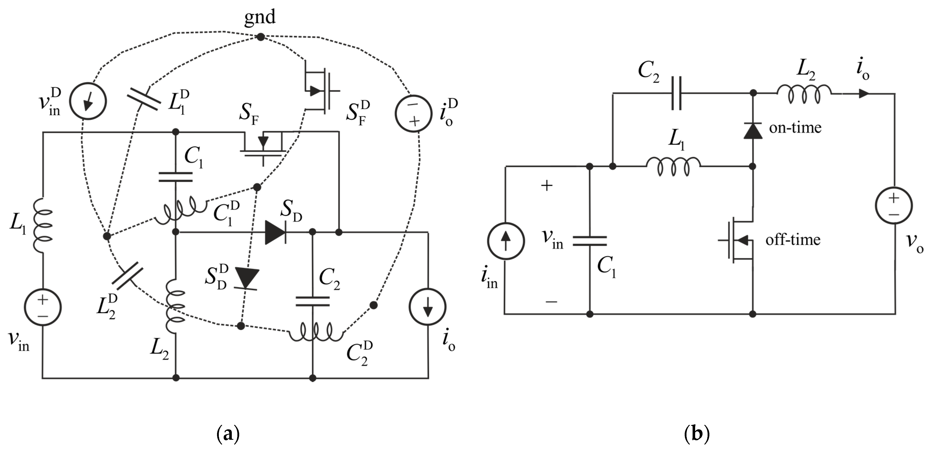
Figure 12.
Buck converter as: (a) voltage-fed converter; and (b) current-fed converter.

Figure 13.
Current-fed buck converter with an input CL filter.

Figure 14.
Cascaded source (S)-converter (C) system.

Figure 15.
Operation modes of single-stage grid-connected PV energy system: (a) grid-feeding/supporting mode; and (b) grid-forming mode.
Figure 15.
Operation modes of single-stage grid-connected PV energy system: (a) grid-feeding/supporting mode; and (b) grid-forming mode.

Figure 16.
Effect of a step change in the duty ratio of an open-loop operated DC-DC converter on PV-generator voltage (dashed line), current (dash-dotted line), and power (solid line) as per-unit curves, when the PV-generator operating point lies in CCR, CPR, and CVR.
Figure 16.
Effect of a step change in the duty ratio of an open-loop operated DC-DC converter on PV-generator voltage (dashed line), current (dash-dotted line), and power (solid line) as per-unit curves, when the PV-generator operating point lies in CCR, CPR, and CVR.

Figure 17.
Measured control-to-output transfer functions () of a boost-power-stage converter operating in CC and CV regions of Raloss SR30-36 PV panel.
Figure 17.
Measured control-to-output transfer functions () of a boost-power-stage converter operating in CC and CV regions of Raloss SR30-36 PV panel.

Figure 18.
Behavior of PV-generator voltage () and current () as well as input-voltage-controlled interfacing-converter output current (), when the operating point of Raloss SR30-36 PV panel is swept from 5 V to 18 V and back.
Figure 18.
Behavior of PV-generator voltage () and current () as well as input-voltage-controlled interfacing-converter output current (), when the operating point of Raloss SR30-36 PV panel is swept from 5 V to 18 V and back.

Figure 19.
Behavior of PV-generator voltage () and current () as well as input-current-controlled interfacing-converter output current (), when the operating point of Raloss SR30-36 PV panel is swept from 18 V to 5 V and back.
Figure 19.
Behavior of PV-generator voltage () and current () as well as input-current-controlled interfacing-converter output current (), when the operating point of Raloss SR30-36 PV panel is swept from 18 V to 5 V and back.

Figure 20.
Measured closed-loop input impedance of an output-voltage-feedback-controlled boost converter.
Figure 20.
Measured closed-loop input impedance of an output-voltage-feedback-controlled boost converter.

Figure 21.
Measured output-voltage loop gain of the boost converter in Figure 19.
Figure 21.
Measured output-voltage loop gain of the boost converter in Figure 19.

Figure 22.
Boost-power-stage converter under output-voltage feedback control.

Figure 23.
Nyquist plot of , where denotes the PV-generator output impedance and denotes the closed-loop input impedance of the voltage-fed boost converter, when the operating point approaches the MPP (16 V) in CVR.
Figure 23.
Nyquist plot of , where denotes the PV-generator output impedance and denotes the closed-loop input impedance of the voltage-fed boost converter, when the operating point approaches the MPP (16 V) in CVR.

Figure 24.
Behavior of boost-converter output voltage () and current () as well as PV-generator voltage (), when the operating point reaches the MPP due to a step change in the output current of the boost converter (i.e., at time ).
Figure 24.
Behavior of boost-converter output voltage () and current () as well as PV-generator voltage (), when the operating point reaches the MPP due to a step change in the output current of the boost converter (i.e., at time ).

Figure 25.
Nyquist plot of , where denotes the PV-generator output impedance and denotes the closed-loop input impedance of the current-fed boost converter, when the operating point approaches the MPP (16 V) in CCR.
Figure 25.
Nyquist plot of , where denotes the PV-generator output impedance and denotes the closed-loop input impedance of the current-fed boost converter, when the operating point approaches the MPP (16 V) in CCR.

Figure 26.
Behavior of boost-converter output voltage () and current () as well as PV-generator voltage (), when the operating point reaches the MPP due to a step change in the output current of the boost converter (i.e., at time ).
Figure 26.
Behavior of boost-converter output voltage () and current () as well as PV-generator voltage (), when the operating point reaches the MPP due to a step change in the output current of the boost converter (i.e., at time ).

© 2017 by the authors. Licensee MDPI, Basel, Switzerland. This article is an open access article distributed under the terms and conditions of the Creative Commons Attribution (CC BY) license (http://creativecommons.org/licenses/by/4.0/).
Share and Cite
MDPI and ACS Style
Suntio, T.; Messo, T.; Aapro, A.; Kivimäki, J.; Kuperman, A. Review of PV Generator as an Input Source for Power Electronic Converters. Energies 2017, 10, 1076. https://doi.org/10.3390/en10081076
AMA Style
Suntio T, Messo T, Aapro A, Kivimäki J, Kuperman A. Review of PV Generator as an Input Source for Power Electronic Converters. Energies. 2017; 10(8):1076. https://doi.org/10.3390/en10081076
Chicago/Turabian StyleSuntio, Teuvo, Tuomas Messo, Aapo Aapro, Jyri Kivimäki, and Alon Kuperman. 2017. "Review of PV Generator as an Input Source for Power Electronic Converters" Energies 10, no. 8: 1076. https://doi.org/10.3390/en10081076
Note that from the first issue of 2016, this journal uses article numbers instead of page numbers. See further details here.