Article

Investigation on the Development of a Sliding Mode Controller for Constant Power Loads in Microgrids

1
Department of Electrical Engineering & Renewable Energy, Oregon Tech, Klamath Falls, OR 97601, USA
2
Department of Mechanical Engineering, University of Wisconsin-Milwaukee, Milwaukee, WI 53211, USA
3
Department of Electrical and Electronics Engineering, University of Johannesburg, Auckland Park 2006, South Africa
4
Department of Industrial Engineering, University of Salerno, 84084 Salerno, Italy
*
Author to whom correspondence should be addressed.
Energies 2017, 10(8), 1086; https://doi.org/10.3390/en10081086
Submission received: 17 May 2017 / Revised: 22 June 2017 / Accepted: 18 July 2017 / Published: 26 July 2017
(This article belongs to the Special Issue Innovative Methods for Smart Grids Planning and Management)

Abstract

:
To implement renewable energy resources, microgrid systems have been adopted and developed into the technology of choice to assure mass electrification in the next decade. Microgrid systems have a number of advantages over conventional utility grid systems, however, they face severe instability issues due to the continually increasing constant power loads. To improve the stability of the entire system, the load side compensation technique is chosen because of its robustness and cost effectiveness. In this particular occasion, a sliding mode controller is developed for a microgrid system in the presence of constant power loads to assure a certain control objective of keeping the output voltage constant at 480 V. After that, a robustness analysis of the sliding mode controller against parametric uncertainties was performed and the sliding mode controller’s robustness against parametric uncertainties, frequency variations, and additive white Gaussian noise (AWGN) are presented. Later, the performance of the proportional integral derivative (PID) and sliding mode controller are compared in the case of nonlinearity, parameter uncertainties, and noise rejection to justify the selection of the sliding mode controller over the PID controller. All the necessary calculations are reckoned mathematically and results are verified in a virtual platform such as MATLAB/Simulink with a positive outcome.

1. Introduction

Microgrid systems deal with several kinds of loads. Based on load function, electrical loads can be classified into two main types: constant voltage loads (CVLs) and constant power loads (CPLs). Traditional loads are of the former category, e.g., incandescent lighting, induction motors, resistive heating, etc. These typically present a constant impedance to the electrical network and are modeled by a resistor or resistor-inductor combination. Since the early days of electrical energy, these have been the only loads which grid operators have faced. However, with the arrival of modern micro/power electronics, non-traditional loads have appeared which do not behave in a similar way in power systems. Non-traditional loads such as switch-mode supplies with regulation, back-to-back converters, electric motor drives, and power electronic circuits fall into this second category called constant power loads. The typical V-I characteristics of a CVL and a CPL are presented in Figure 1 below. Today’s devices require strict control and regulation of the operating parameters to function properly. Strictly regulated point-of-load converters mean that the power output of these devices will remain constant, even though the input voltage changes. The use of active rectifiers is becoming the preferred interface for loads in distribution systems in response to the increasing concerns about power quality issues [1,2].
As electronic loads increase, the proportion of CPLs in the overall load will rise. This change in proportion brings about problems in system stability due to the CPL characteristics [3,4]. While these problems were known before, the fraction of CPL was too small to cause much concern, but with changes in electrical energy distribution and consumption occurring worldwide, these problems now require further investigation. CPLs cause a significant amount of instabilities in converter-based power systems due to their negative impedance characteristics. Microgrids incorporate multiple converter stages in cascade and have to follow stringent point-of-load regulations. These factors coupled with the poorly damped architecture of microgrids, makes them seriously vulnerable to CPL instabilities. The microgrid bus voltage becomes unstable, oscillating randomly, and these problems increase exponentially in nature because of CPLs. Without application of a proper control technique, such instability can lead to momentary brown outs, or longer lasting black outs. Since the last decade, a great deal of research has been done to overcome the CPL instability issue [5], but none has been able to provide the comprehensive solution of this phenomenon with a sensitivity analysis of the entire system and appropriate compensation techniques for microgrid application. Therefore, more research is still required in this field [6,7].
To improve the stability scenario of the microgrid system, several linear and nonlinear control techniques have already been adopted [8,9]. Besides that, researchers and professionals have been conducting cutting-edge research to enhance the system stability around the world [10]. In the case of DC microgrids, a number of related studies are reviewed in [11,12,13]. After investigating a number of research works on stability issues in microgrids, where the majority of the loads are installed with CPL, we come to the conclusion that CPL instability compensation techniques can be classified into three groups. These are: (i) feeder side compensation; (ii) compensation by adding intermediate circuitry; (iii) load side compensation [14]. It is evident if CPL compensation is done on the load side, the system doesn’t experience the effect of constant power loads. Loads and generation tend to coincide in microgrid systems; therefore, load side management appears as a key stabilization technique. This method has additional advantages as it can be applied at any intended point, and is quite unmatched in overcoming the instabilities caused by loads incorporating both CPL and CVL. Furthermore, the load side compensation arrangement can be made a portable system, giving it a distinct advantage over feeder side or intermediate compensation techniques. The load side compensation technique offers better robustness as well as cost effectiveness. For a nonlinear system such as a microgrid, there are numerous applicable nonlinear control systems: describing function method, singular perturbation method, Lyapunov stability analysis, phase plane method, Popov criterion, small-gain theorem, center manifold theorem, gain scheduling, passivity analysis, Lyapunov redesign, feedback linearization, backstepping, nonlinear damping, and sliding mode control (SMC). Among all these nonlinear control systems, SMC is chosen because of the advantages it offers. This control system is capable of switching among different continuous structures according to the position in state space, which makes it a variable structure control mode. However, SMC’s main strength lies in its robustness and impermeability to parameter variations as well as noise. The switching of states in this method can be switching between quite simple states such as on and off. Therefore, this method need not be precise to achieve satisfactory results. The control law not being a continuous function, sliding mode can be attained in finite time. These characteristics make SMC the optimal control system for a wide range of dynamic structures. Moreover, in the case of converters with discrete operating modes such as a microgrid system, discrete SMC becomes a natural choice over the continuous controller arrangement which will need an intermediate system (e.g., pulse width modulation) to be applied.
Hence, in this paper, the SMC technique will be implemented in the case of load side compensation for CPL instability in microgrid systems. The combined advantages of SMC and load side compensation make this approach as strong as it gets. However, it cannot escape from the drawbacks that come with SMC. Because of the imperfections and delays of actuators, application of SMC can lead to energy loss, chatter, and excitement of unmodeled dynamics. Therefore, this proposed system needs more care than any other nonlinear control system. Before this, some research works have been accomplished by the sliding mode control technique. With large systems, the stability characteristics become more difficult to establish. To use the original, non-linear models of the system, SMC has been implemented in DC microgrids [15,16,17] by finding a sliding surface and using a discontinuous sliding mode controller to improve voltage stability. In a similar manner, a non-linear sliding surface is proposed by Singh and Fulwani, two researchers from the Indian Institute of Technology Jodhpur [18] to mitigate CPL instability. Their proposed non-linear surface confirmed that the constant power was maintained, in practice, by the converter. Thus, the proposed controller was necessarily able to mitigate the CPL’s oscillating effect of tightly regulated Point of Loads (POL) and assure the stable operation of DC microgrids under a number of disturbances. Apart from that work Gautam et al. have presented a robust sliding mode control technique to investigate CPL instability [19]. After that, in [20], Stramosk and Pagano proposed a novel sliding mode controller to control the DC bus voltage precisely. In the case of a AC microgrids, a number of studies are reviewed in [21,22,23]. Using all the background knowledge of this research, the cardinal objective of this paper was to develop a novel sliding mode controller for microgrids with constant power loads [24,25].
This paper offers some unique contributions as it applies SMC for load side compensation to mitigate the instabilities caused by CPLs in microgrids, which is not done in the works stated above. Furthermore, performance of the proposed system is analyzed in simulation and is compared to a proportional integral derivative (PID) control system, which is widely employed in similar industrial operations. PID control systems are a linear control technique; they work at a fixed operating point, which is impractical in nonlinear systems such as microgrids. In renewable resource-based microgrid systems, parameters change, and noise gets added all the time. To apply PID control in such systems, they have to be linearized, which does not provide the exact operating point that PID requires; and lots of system properties are also lost. Therefore, nonlinear control systems are better suited than PID control systems to handle the instability of microgrid systems, and as stated above, this proposed method employing SMC is the best choice among the nonlinear control systems. This statement is demonstrated through simulation results in this paper, along with the other findings, and is one of its major contributions.
In this paper, in Section 2, constant power load (CPL) instability is presented with necessary examples. After that, in Section 3, the sliding mode control (SMC) technique is introduced. In this Section, the control principle of SMC, chattering, chattering reduction, advantages of SMC, controller design, and control objectives are delineated with necessary equations and depictions. In Section 4, the robustness analysis of SMC is presented. After that, in Section 5, results and simulations are illustrated in the case of a number of system parameters between robustness analysis against parametric variation and robustness analysis against parametric uncertainties, frequency variation and additive Gaussian noise using SMC control technique based on boundary condition.
The contributions of this paper are as follows: development of a sliding mode controller for microgrids with constant power load to assure control objectives/desired output. The robustness of the sliding mode controller against parametric uncertainties is presented. Besides that, the sliding mode controller robustness against parametric uncertainties, frequency variations and additive white Gaussian noise (AWGN) will be illustrated. Finally, the performance of the PID and SMC techniques will be compared to microgrid output voltage in the case of nonlinearity, parameter uncertainties, and noise rejection.

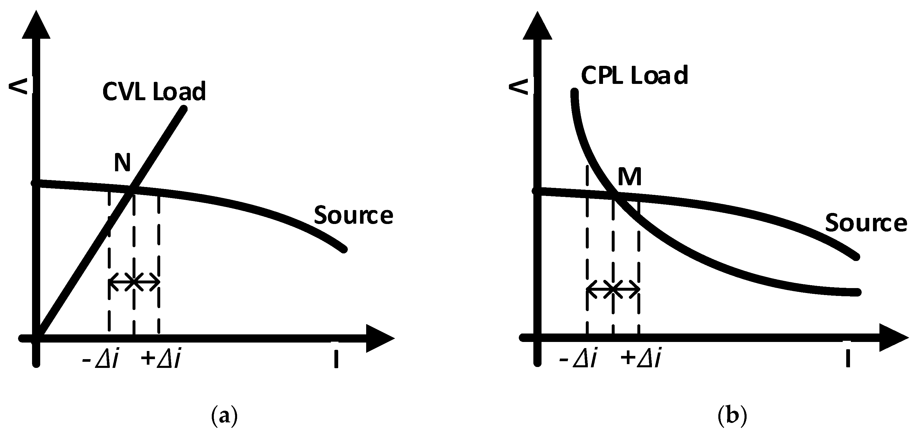
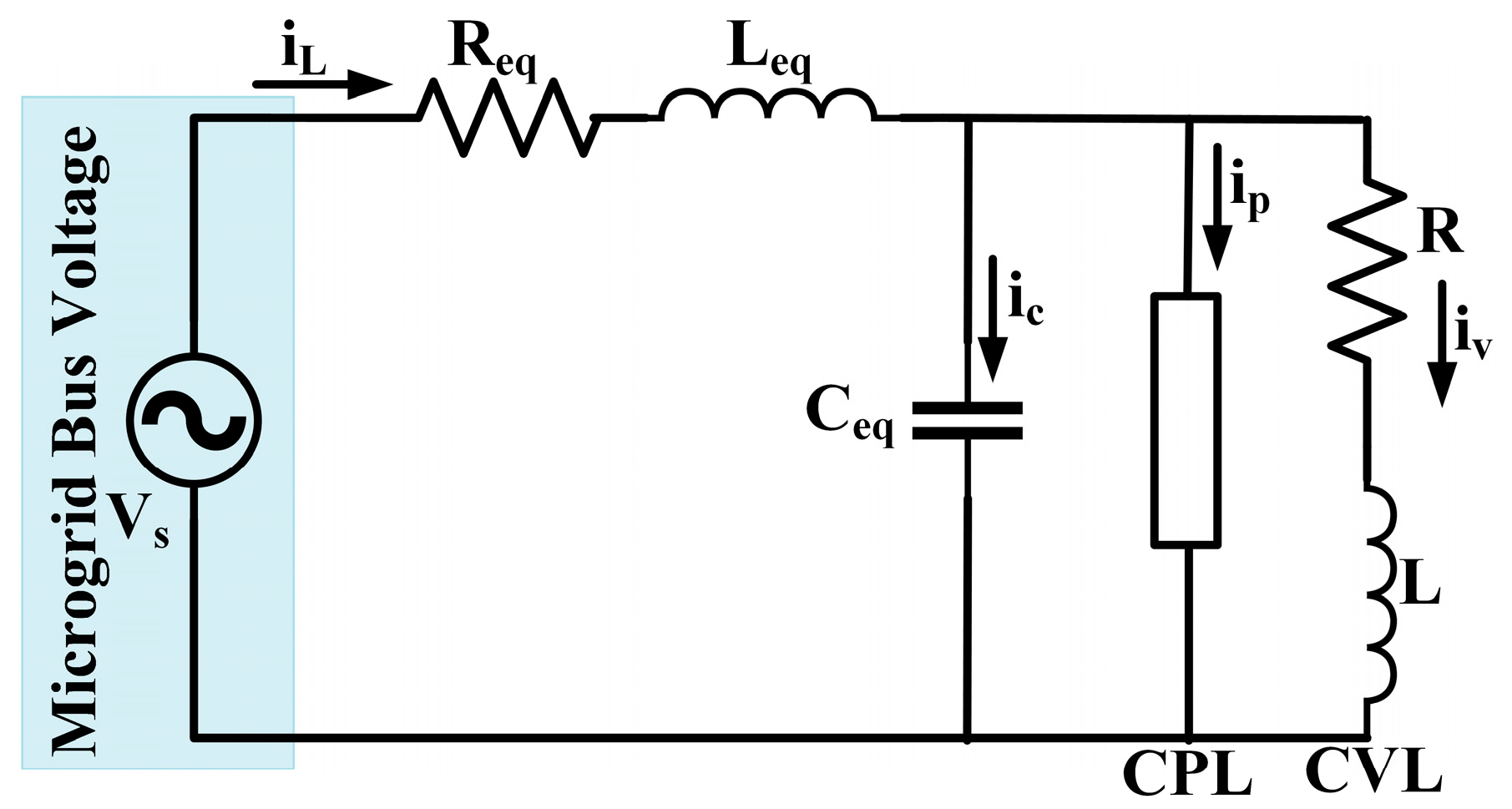
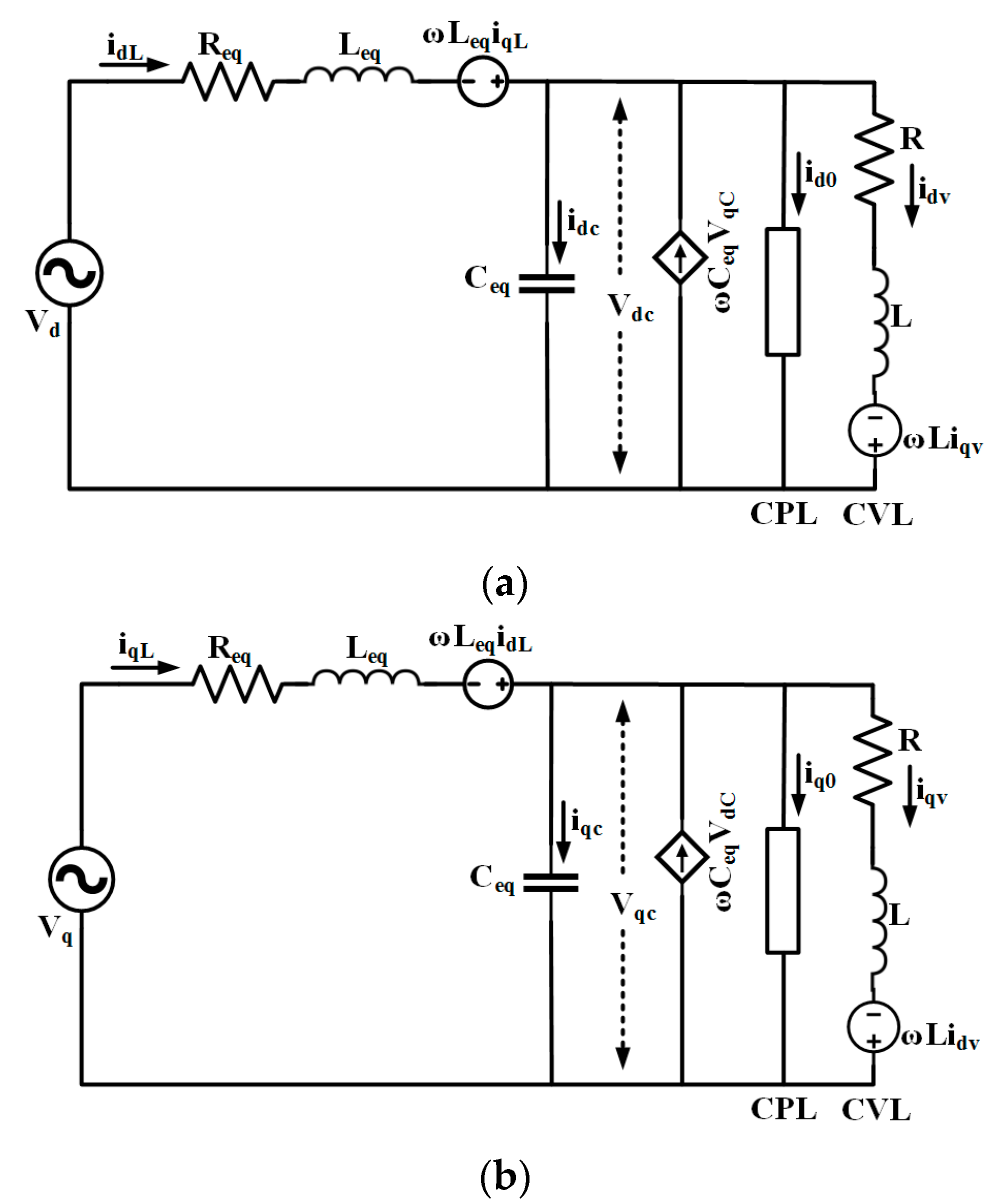
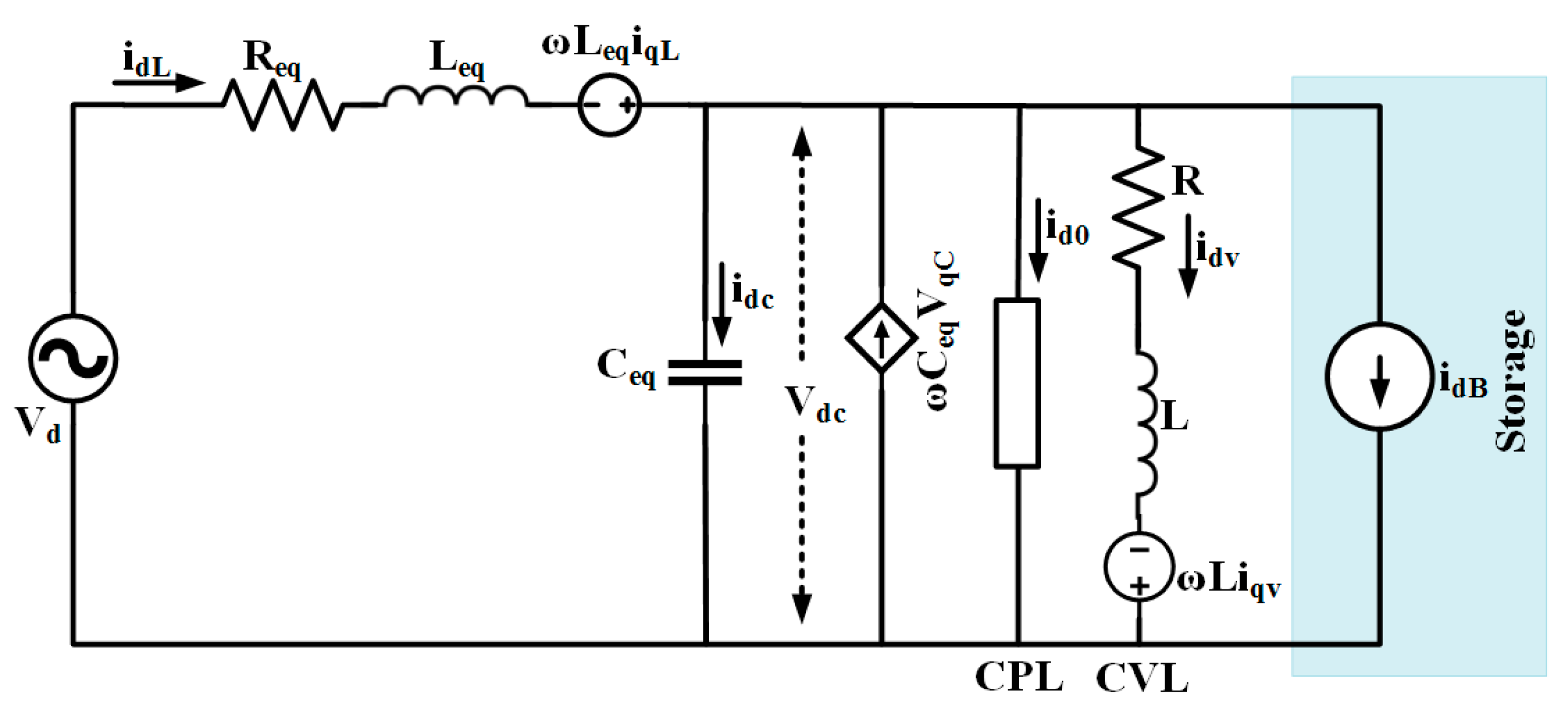
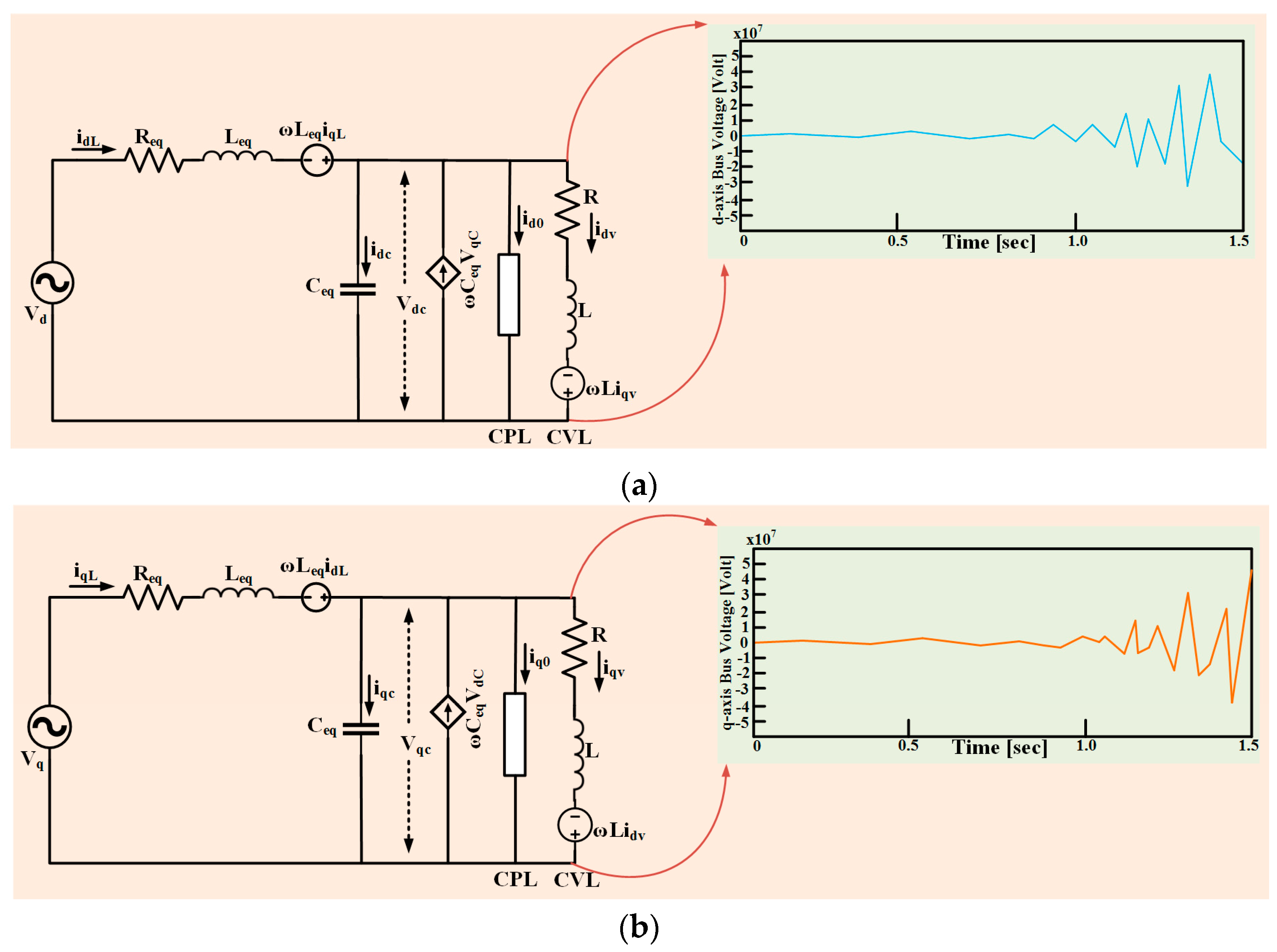
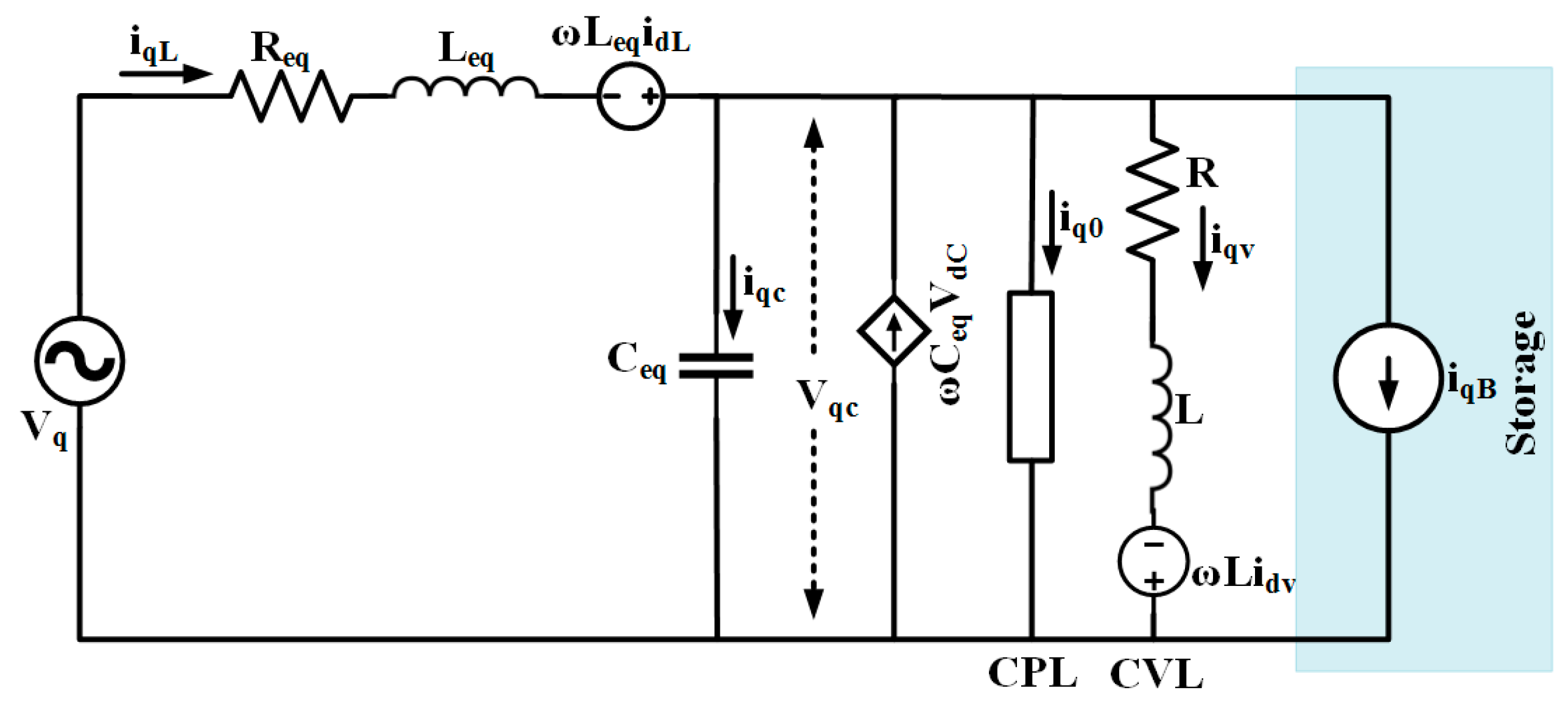
2. Modeling of Microgrid with CPL

The small signal equivalent model of the microgrid is represented in Figure 2. Here Vs represents the combined voltage output from the sources of the microgrid. In this paper, source types are not specified and Vs is used as an equivalent of any source that can be used in a practical microgrid. As the renewable sources are intermittent in nature, Vs is modeled as a varying source to simulate that. Req, Leq, and Ceq represent the equivalent transmission line resistance, inductance, and capacitance from source to load. The loads: CPL and CVL, are connected to the transmission line in parallel.
To develop a mathematical model of the loads from circuit shown in Figure 2, taking Leq = L1, Req = R1, Ceq = C for simplicity and applying circuit theorem gives:
d i L d t   =     R 1 L 1   i L     1 L 1 V C   +   V s L 1 ,
d V C d t   +   P O V C   +   i V   =   i L ,
By taking output current io as a function of capacitor voltage VC i.e., i o = P o V C ; where Po is the Power of constant power load (CPL) and also a constant gives Equations (3) and (4):
d V C d t   =   1 C i L     1 C P o V C     1 C i V ,
d i V d t   =   1 L V C     R L i V ,
To develop the nonlinear state-space model, the state variables are defined as x1 = iL, x2 = VC, x3 = iV, and the system input voltage as VS; which gives Equation (5):
[ x 1 ˙ x 2 ˙ x 3 ˙ ]   =   [ R 1 L 1 x 1     1 L 1 x 2   +   1 L 1 V S 1 C x 1     1 C P O x 2     1 C x 3 1 L x 2     R L x 3 ] ,
The equivalent d-q axis model circuit is represented in Figure 3a,b. Using d-q transformation matrix:
i d L   =   2 3 [ i a L cos ω t   +   i b L cos ( ω t     120 )   +   i c L cos ( ω t   +   120 ) ] ,
Therefore:
d i d L d t   =   2 3 [ d i a L d t cos ω t   +   d i b L d t cos ( ω t     120 )   +   d i c L d t cos ( ω t   +   120 ) ]     2 3 ω [ i a L sin ω t   +   i b L sin ( ω t     120 )   +   i c L sin ( ω t   +   120 ) ] ,
i q L   =   2 3 [ i a L sin ω t   +   i b L sin ( ω t     120 )   +   i c L sin ( ω t   +   120 ) ] ,
Therefore, it can be stated that:
d i d L d t   =   ω i q L     R 1 L 1 i d L     V d c L 1   +   V d L 1 ,
Similarly:
d i q L d t   =     ω i d L     R 1 L 1 i q L     V q c L 1   +   V q L 1 ,
Again from Equation (1), using d-q transformation:
d V d C d t   =   ω V q C   +   1 C i d L     1 C   P o V d C     1 C i d V ,
d V q C d t   =   ω V d C   +   1 C i q L     1 C   P o V q c     1 C i q V ,
From Equation (4), using d-q transformation:
d i d V d t   =   ω i q V   +   1 L V d C     R L i d V ,
d i q V d t   =   ω i d V   +   1 L V q C     R L i q V ,
d-q transformed state equations from Equation (9) to (14):
[ d i d L d t d i q L d t d V d C d t d V q C d t d i q V d t d i q V d t ] = [ ω i q L     R 1 L 1 i d L     V d c L 1   +   V d L 1 ω i d L     R 1 L 1 i q L     V q c L 1   +   V q L 1 ω V q C   +   1 C i d L     1 C   P o V d C     1 C i d V ω V d C   +   1 C i q L   1 C   P o V q c     1 C i q V ω i q V   +   1 L V d C   R L i d V ω i d V   +   1 L V q C   R L i q V ] ,
For the ease of controlling uncompensated nonlinear systems and presenting a detailed analysis of state variables to implement the advanced nonlinear control algorithms, we have derived d-q axis modeling of the designed system. The equivalent d-q axis model circuit is represented in Figure 3a,b. When we consider line frequency is 60 Hz, then ω (speed term) becomes static. However, in practical cases, line frequency always fluctuates, which depends on various characteristics of the system, so in those cases, ω (the speed term) becomes dynamic and nonlinear.
d-q transformed state equations can be represented by Figure 3 as:
[ d i d L d t d i q L d t d V d C d t d V q C d t d i d V d t d i q V d t ] = [ ω i q L     R 1 L 1 i d L     V d c L 1   +   V d L 1 ω i d L     R 1 L 1 i q L     V q c L 1   +   V q L 1 ω V q C   + 1 C i d L   1 C   P O V d C 1 C i d V ω V d C + 1 C i q L   1 C   P O V q c 1 C i q V ω i q V + 1 L V d C   R L i d V ω i d V + 1 L V q C   R L i q V ] ,
Using Equation (16), the bus voltage instability of d-axis due to the constant power loads is presented schematically in Figure 4. In this case, an abrupt and random change is observed in the d-axis bus voltage.
In this sequence, the bus voltage instability of q-axis due to the constant power loads is presented in Figure 5. Like the d-axis bus voltage, the exponentially increased signal and random oscillation are also demonstrated in the case of the q-axis bus voltage.
In the following illustration, the entire design of the microgrid arrangement loaded with CPLs is depicted for d-q representation in Figure 6. The figure exhibits the undamped oscillation due to the perturbation created by the CPL loads in case of microgrid d axis and q axis bus voltage. This disturbance in both of the output voltages leads to the undesired voltage collapse in the microgrid system.
To mitigate this perturbation due to CPL loads, the load side compensation technique is reasonably adopted rather than the feeder side compensation and the intermediate circuitry compensation technique. In the load side compensation technique, necessary manipulation is made in load side of the system so that the system doesn’t experience the effect of constant power loads. To clarify this technique, the real power compensation and reactive power compensation technique are modeled below schematically in Figure 7 and Figure 8.
From the above dq-axis modeling, the combined state space equation of the adopted load side compensation technique is presented in Equation (17):
[ d i d L d t d i q L d t d V d C d t d V q C d t d i d V d t d i q V d t ] = [ ω i q L R 1 L 1 i d L V d c L 1 + V d L 1 ω i d L R 1 L 1 i q L V q c L 1 + V q L 1 ω V q C   +   1 C i d L   1 C   P O V d C     1 C i d V 1 C i d B ω V d C   +   1 C i q L   1 C   Q O V q c     1 C i q V 1 C i q B ω i q V   +   1 L V d C   R L i d V ω i d V   +   1 L V q C   R L i q V ]

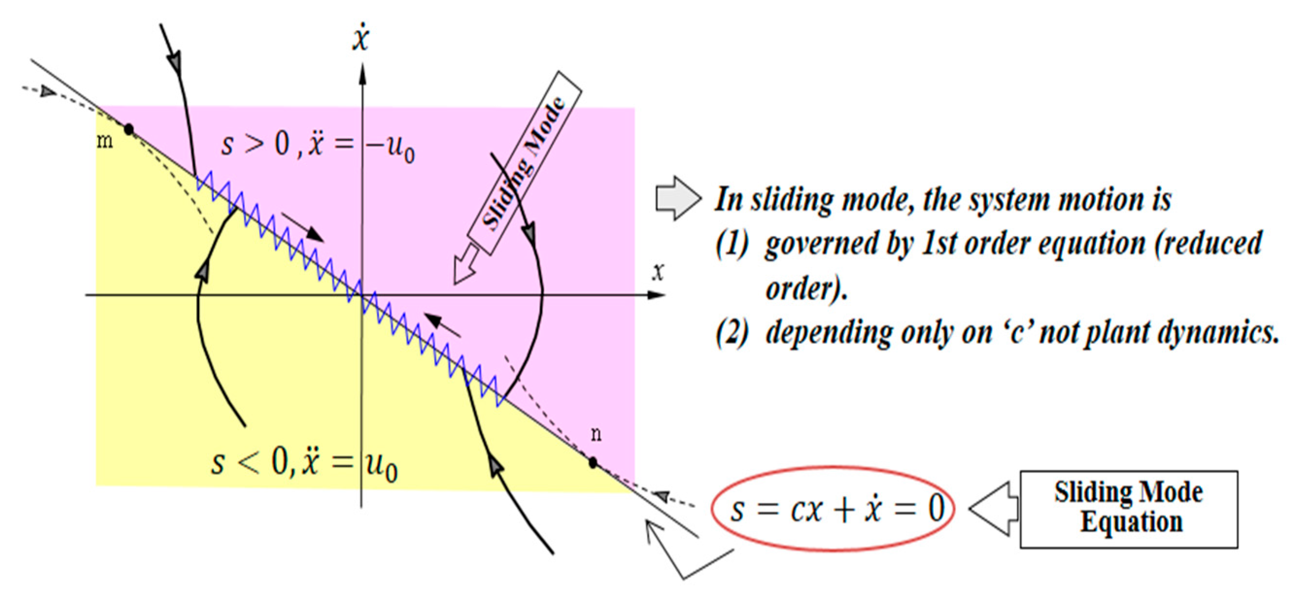
3. Sliding Mode Controller Design

Sliding mode control, commonly known as the SMC technique, is an advanced nonlinear control strategy that features salient properties of accuracy, robustness, and easy tuning and adjusts the system dynamics by the function of discontinuous control signal, forcing the system output to ‘slide’ along with sliding surface or a defined cross-section of the system’s nominal behavior [27]. Here, the state feedback control law, a discontinuous function of time, can shift from one structure to another (in a continuous manner) based on the prevailing location in the space. Therefore, the SMC can be defined as a variable structured control technique. The certain operation mode of the system, as it slides along the predefined boundaries of the control structures, is called the sliding mode. Besides that, the geometrical locus, necessarily consisting of the boundaries, is said to be the sliding surface of the system. Here, Figure 9 depicts an instance of the trajectory of a certain system regarding the SMC technique. In this illustration, the sliding surface is defined by, s = 0, and, in this occasion, the sliding mode starts after a finite time while the system trajectories have come to the specified surface.
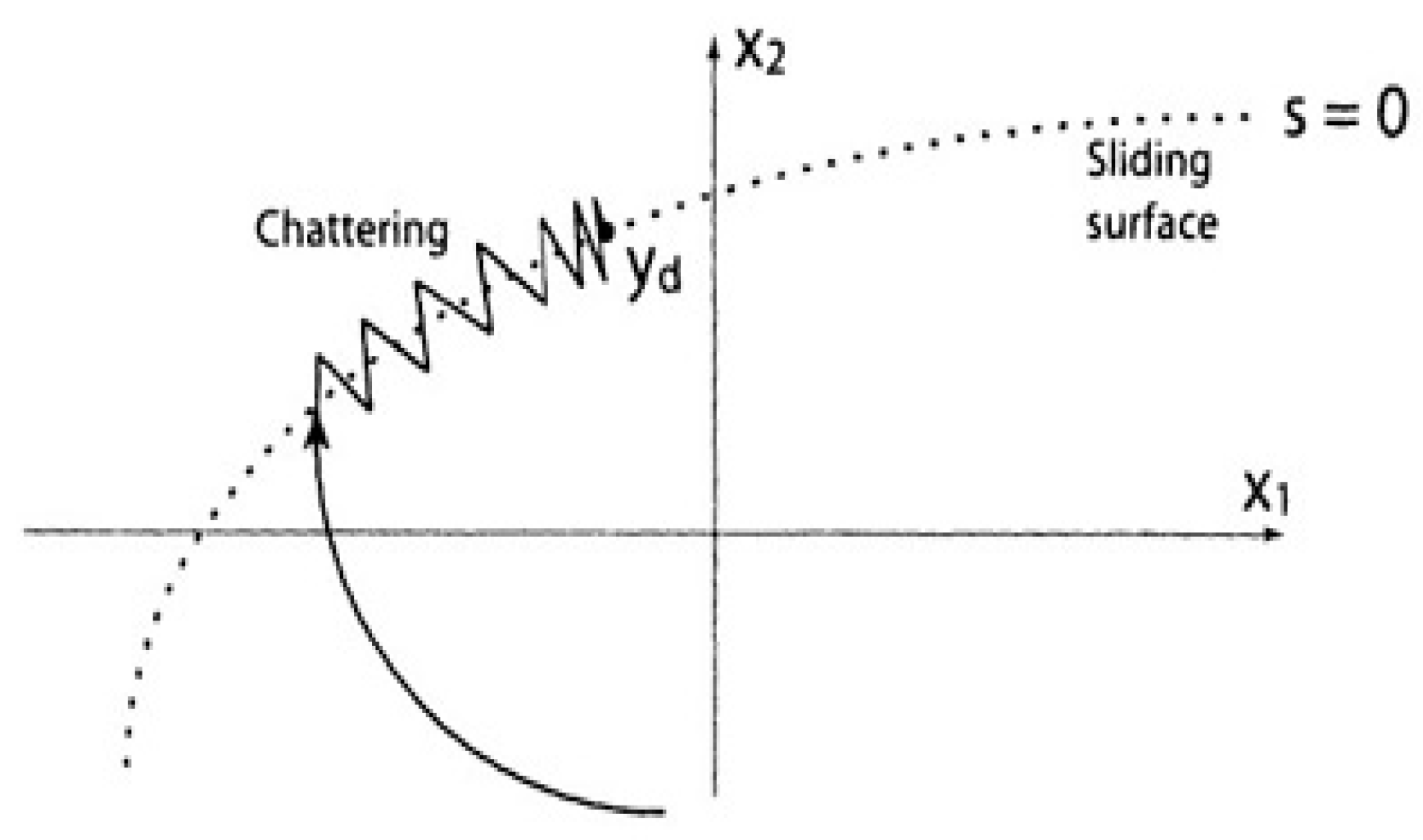
  • State trajectories are toward the switching line s = 0
  • State trajectories cannot leave and belong to the switching line s = 0
  • After sliding mode starts, further motion is governed by s   =   c x   +   x ˙ =   0

3.1. Chattering

The absolute sliding mode remains only while the state trajectory x(t) of the controlled plant complies with the coveted trajectory at each t ≥ t1 for some value of t1 [29]. Here, it may need the infinitely rapid switching, but in the practical systems case, the switching controller does have a number of inadequacies that actually confines switching up to a definite frequency. In this occasion, then the representative point oscillates within a predefined neighborhood of the switching surface. In particular, this kind of oscillation is said to be the chattering [30]. This phenomenon is presented in Figure 10.

3.2. Chattering Reduction

Control laws which satisfying the sliding condition (the simplified 1st order problem of keeping the scalars at zero can be achieved by choosing the control law u such that outside of s(t) as ½*d/dt(s2) ≤ –η|s|, where η is a strictly positive constant) and lead to “perfect” tracking in the face of model uncertainty, are discontinuous across the surface s(t), thus causing control chattering. Chattering is undesirable for the designers because it demands extremely high control activity, and furthermore it involves with the high-frequency dynamics which is neglected in the course of modeling. Chattering must be reduced (eliminated) for the controller to perform properly. This can be achieved by smoothing out the control discontinuity in a thin boundary layer neighboring the switching surface in Equation (18):
B ( t )   =   { x , | s ( x , t ) |     }     >   0   B ( t )   =   { x , | s ( x , t ) |     }     >   0 ,
t     0 , |   x ˜ i   ( t ) | 2 λ i   ε ,   I   =   0 , ( n     1 ) ,
where is boundary layer thickness, ε is tracking precision.

3.3. Selection of Sliding Mode Control over PID Control Technique

PID control technique is one of the most popular and frequently used linear control techniques around the world, but in the case of microgrid applications, to retain the desired stability despite the negative incremental load characteristics of CPL, some inconveniences occur due to the lack of accuracy consistency. Unlike the PID controller, the sliding mode control technique has been developed into the preferable choice to researchers because of its success in practical cases, desired consistency, and straightforward firmware implementation. Besides that, the sliding mode control technique generates discontinuous on/off signals that necessarily force the system to slide along the desired system’s behavior. An SMC controller utilizes a discrete sliding decision rule to retain the desired output. According to this, the system, adopting SMC technique, flows through both continuous and discrete modes. By this way, it demonstrates a hybrid feedback configuration in practice. Sliding mode control technique has a number of advantages over the conventional PID control technique. Hence, in this paper, the sliding mode control technique has been adopted to improve the stability of the microgrid system in the presence of CPL loads. The advantages of the SMC control technique are listed below to compare these two techniques:
  • Characteristically, the microgrid system is significantly nonlinear with time-varying parameters as well as system uncertainties. Hence, using PID control technique may hamper system stability due to the possible overlinearization of the system. On the other hand, an SMC controller doesn’t ignore the system nonlinearity during controller design.
  • The efficiency of the entire system depends cardinally on the loading conditions. In the case of modeling imprecision, the SMC controller offers a systematic way to address the complication of retaining stability as well as the desired consistent performance.
  • The sliding mode control technique is easy to implement. It requires implementation of short computational and numerical algorithms in the microcontroller. It is readily compatible with the standard communication protocols such as Ethernet/IP, RS-232, and the Modbus.
  • In the case of harsh industrial environments, where stability, as well as high performance, is required despite the presence of high nonlinearity, the lifetime of the hardware components can be reduced considerably in the application of PID controllers. Unlike the PID control technique, SMC requires significantly less equipment and maintenance costs.
  • Compared to the PID control technique, SMC offers robust performance against parametric variations and any disturbance and better response time to retain microgrid stability.

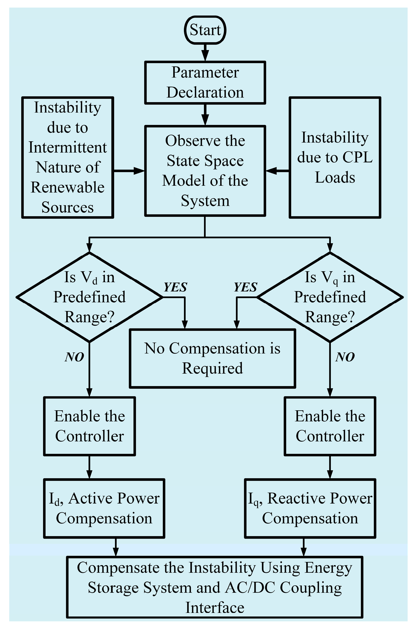
3.4. Controller Design

Two steps have to be followed according to the controller design procedure. Initially, it is required to select a feedback control law u to verify the sliding condition. Nevertheless, the control law has to be discontinuous across s(t) to account for the existence of the modeling imprecision as well as of perturbations. As the consequence of the imperfection of associated control switching, it contributes to chattering (see Figure 10). In practice, chattering is absolutely undesirable for the system, since this requires a special control scheme. Besides that, it may introduce high-frequency dynamics that were neglected in the modeling purpose case. After that, in the next step, the discontinuous control law u is to be suitably smoothed to achieve an optimal condition in the course of the trade-off between the control bandwidth and tracking precision [32]. Therefore, the first step assures the desired robustness for the parametric uncertainty as well as perturbations, and the second step offers robustness to the high-frequency unmodeled dynamics. The illustrated design steps of the SMC controller are discussed for the microgrid system [33]. Here, we present the modified controller model of microgrid systems to implement the storage-based virtual impedance stabilization technique using SMC controller.

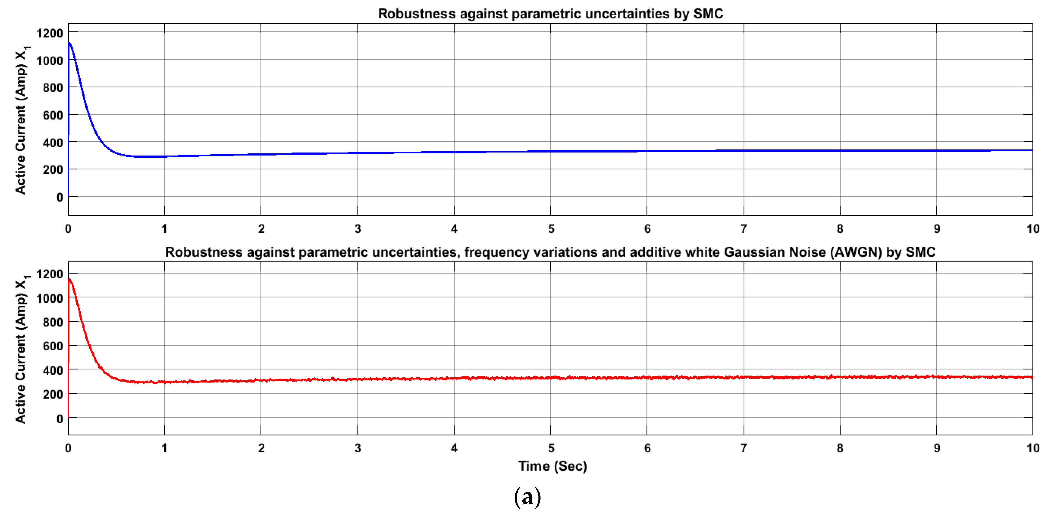
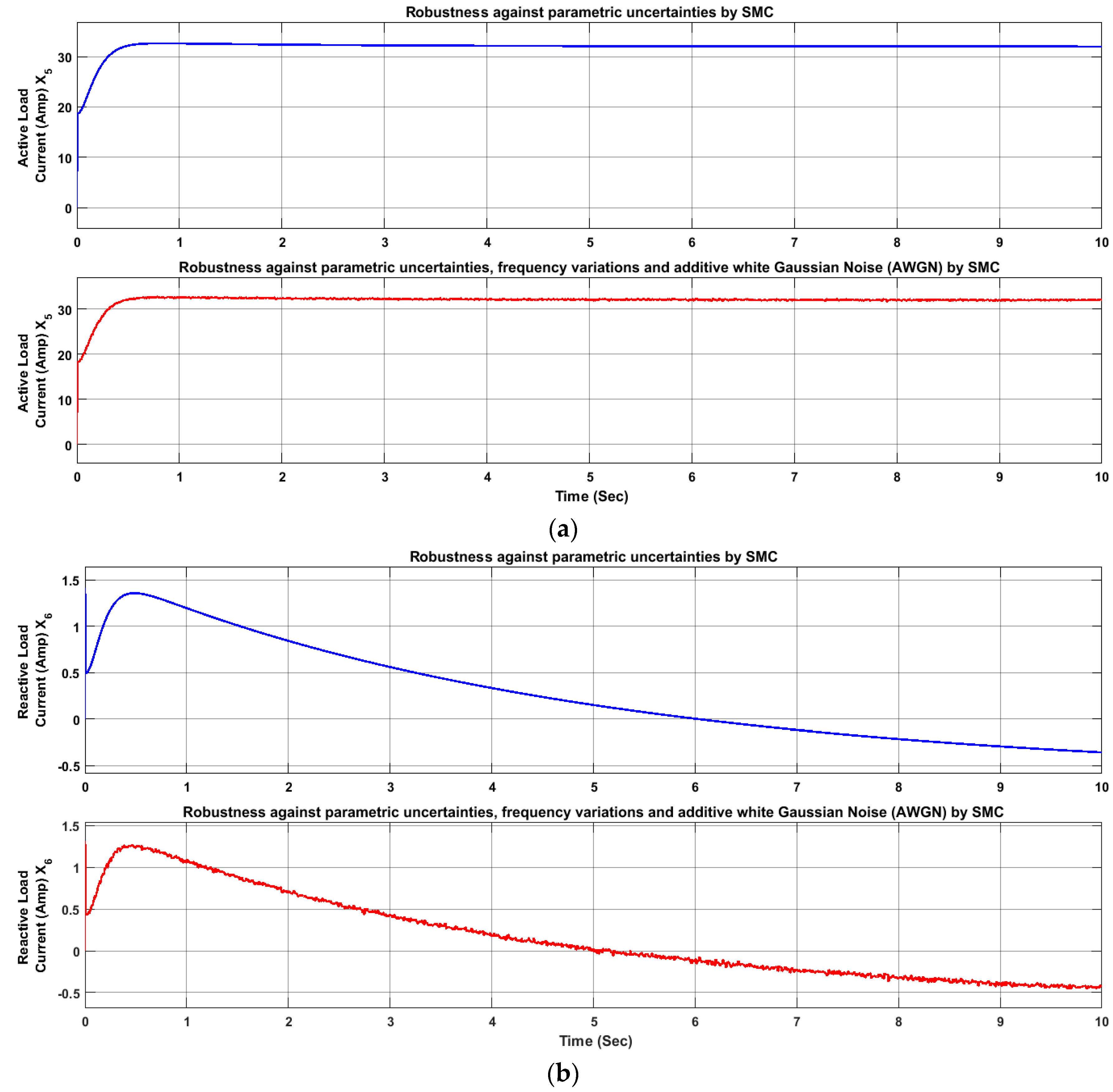
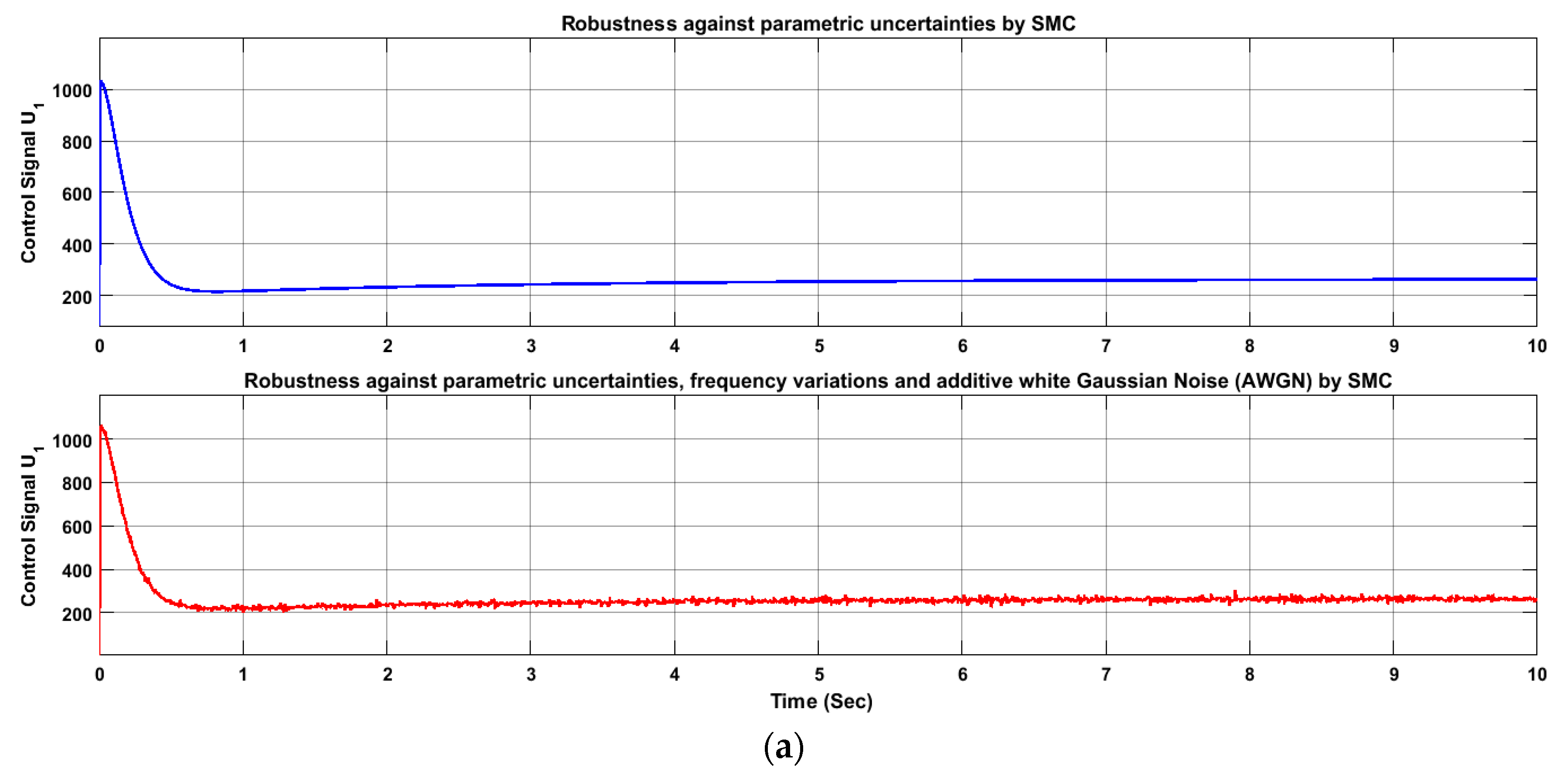
4. Robustness Analysis of SMC

Here, the control objectives/desired output of the proposed controller are Y1 = VdCVd ≈ 480 V and Y2 = VqCVq ≈ (as low as possible) V.
The general form of a system which is affine in the control(s) is given by Equation (20) [34,35,36,37,38,39]:
x ˙   =   f ( x )   +   g ( x ) u ,

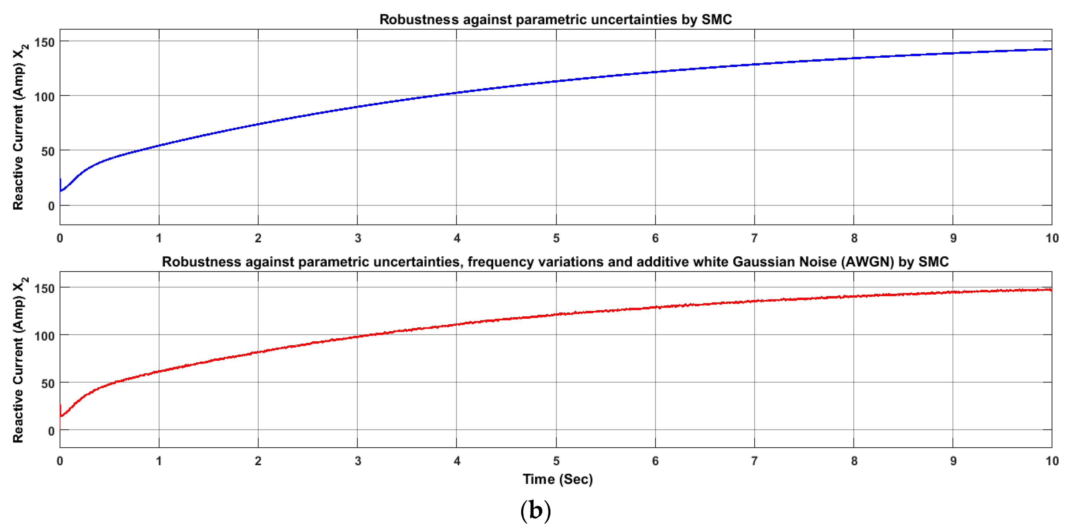
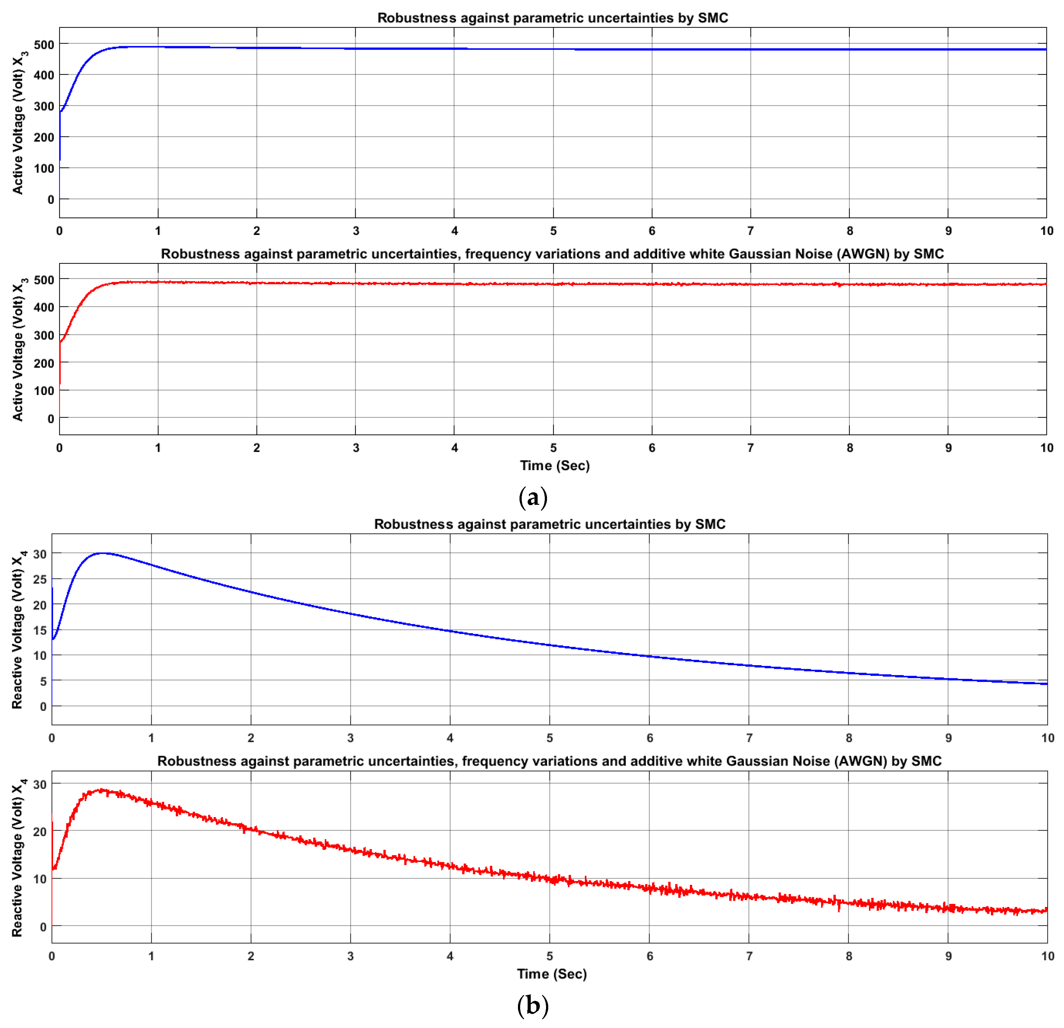
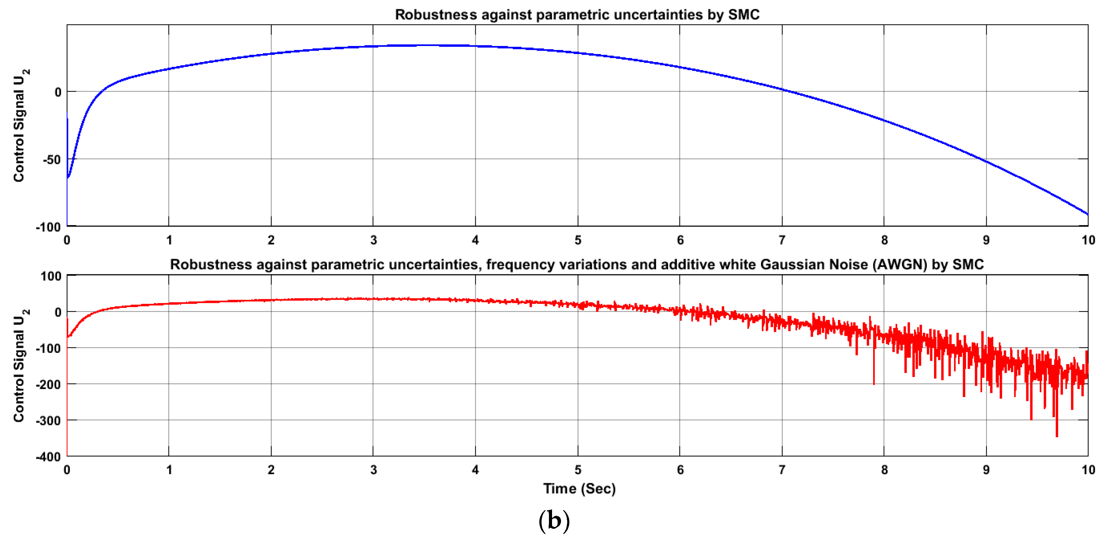
4.1. Sliding Mode Controller, Robustness Against Parametric Uncertainties

We can rewrite our state space model equation as Equation (21) below [39,40,41,42,43,44,45]:
[ x 1 ˙ x 2 ˙ x 3 ˙ x 4 ˙ x 5 ˙ x 6 ˙ ] = [ ω x 2     R 1 L 1 x 1     x 3 L 1 ω x 1     R 1 L 1 x 2     x 4 L 1 ω x 4 + 1 C x 1   1 C P O x 3 1 C x 5 ω x 3 + 1 C x 2   1 C Q O x 4 1 C x 6 ω x 6 + 1 L x 3   R L x 5 ω x 5 + 1 L x 4   R L x 6 ] + [ 0 0 1 C u 1 1 C u 2 0 0 ] + [ r 1 L 1 r 2 L 1 0 0 0 0 ] ,
where, r 1 and r 2 are unknown parameters that satisfy r 1 δ r 1 and r 2 δ r 2 for some known bounds δ r 1 and δ r 2 . Our goal is to regulate the output active voltage x 3 and reactive voltage x 4 by designing the control laws u 1 and u 2 respectively. As x 3 and x 4 are related to r 1 and r 2 through x 1 and x 2 respectively. So, x 1 and x 2 are also unknown parameters those satisfy Δ x 1     δ x 1 and Δ x 2     δ x 2 for some known bounds δ x 1 and δ x 2 . We will design sliding mode control input, u 1 in the first attempt and then we will follow the similar method to design another control input u 2 .
To make the integral controller, let:
e 1   =   ( x 3     x 3 d ) d t ,
e 2   =   e ˙ 1   =   x 3     x 3 d ,
e ˙ 2   =   x ˙ 3     x ˙ 3 d   =   f 3 ( x ) +   g 3 ( x ) u 1     x ˙ 3 d ,
Expanding f 3 ( x ) and g 3 ( x ) :
e ˙ 2   =   ω x 4   +   1 c x 1     1 c P 0 x 3     1 c x 5     1 c u 1     x ˙ 3 d ,
Let the sliding surface be:
s   =   e 1   +   e 2 ,
Then, its derivative will be:
s ˙   =   e ˙ 1   +   e ˙ 2 ,
s ˙   =   e 2   +   ( ω x 4   +   1 c x 1     1 c P 0 x 3     1 c x 5     1 c u 1     x ˙ 3 d ) ,
The state x 1 is unknown, then we can represent the uncertainty as x 1   =   x ^ 1   +   Δ x 1 and:
| | 1 c Δ x 1 | |     1 c δ x 1   =   e 2   +   ( 1 c x 5     x ˙ 3 d     1 c P 0 x 3   +   ω x 4   +   1 c x ^ 1   +   1 c Δ x 1     1 c u 1 ) ,
Let this be the Lyapunov candidate function:
V   =   1 2 s 2 ,
V ˙ =   s s ˙ =   s ( e 2   +   ( 1 c x 5     x ˙ 3 d     1 c P 0 x 3   +   ω x 4   +   1 c x ^ 1   +   1 c Δ x 1     1 c u 1 ) ,
We use u 1 as:
u 1   =   c [ e 2   +   1 c x 5   +   x ˙ 3 d   +   1 c P 0 x 3     ω x 4     1 c x ^ 1   +   v ] ,
Then, we can obtain:
V ˙   =   s ( 1 c Δ x 1   +   v ) ,
Considering | | 1 c Δ x 1 | |     1 c δ x 1 , the following discontinuous control, v , will make V ˙ to be negative, and consequently, guarantee stability:
v   =   1 c δ x 1 s a t ( s ε ) ;   ε   >   0 ,
Totally, the control input is:
u 1   =   c [ e 2   +   1 c x 5   +   x ˙ 3 d   +   1 c P 0 x 3     ω x 4     1 c x ^ 1     1 c δ x 1 s a t ( s ε )   ] ,
Like u 1 , let:
e 3   =   ( x 4     x 4 d ) d t ,
e 4   =   e ˙ 3   =   x 4     x 4 d ,
e ˙ 4   =   x ˙ 4     x ˙ 4 d   =   f 4 ( x ) +   g 4 ( x ) u 2     x ˙ 4 d ,
Expanding f 4 ( x ) and g 4 ( x ) :
e ˙ 4   =   ω x 3   +   1 c x 2     1 c Q 0 x 4     1 c x 6     1 c u 2     x ˙ 4 d ,
Let, the sliding surface be:
s   =   e 3   +   e 4 ,
s ˙   =   e ˙ 1   +   e ˙ 2 ,
Then, its derivative will be:
s ˙   =   e ˙ 3   +   e ˙ 4 ,
s ˙   =   e 4   +   ( ω x 3   +   1 c x 2     1 c Q 0 x 4     1 c x 6     1 c u 2     x ˙ 4 d ) ,
The state x 2 is unknown, then we can represent the uncertainty as x 2   =   x ^ 2   +   Δ x 2 and:
| | 1 c Δ x 2 | |     1 c δ x 2   =   e 4   +   ( ω x 3   +   1 c x ^ 2     1 c Q 0 x 4     1 c x 6     x ˙ 4 d   +   1 c Δ x 2     1 c u 2 ) ,
Let this be the Lyapunov candidate function:
V   =   1 2 s 2 ,
V ˙ =   s   s ˙ =   s ( e 4   +   ( ω x 3   +   1 c x ^ 2     1 c Q 0 x 4     1 c x 6     x ˙ 4 d   +   1 c Δ x 2     1 c u 2 ) ) ,
We use u 2 :
u 2   =   c [ e 4   +   ω x 3     1 c x ^ 2   +   1 c Q 0 x 4   +   1 c x 6   +   x ˙ 4 d   +   v ] ,
Then, we can obtain:
V ˙   =   s ( 1 c Δ x 2   +   v ) ,
Considering | | 1 c Δ x 2 | |     1 c δ x 2 , the following discontinuous control, v , will make V ˙ to be negative, and consequently, guarantee stability:
v   =   1 c δ x 2 s a t ( s ε ) ;   ε   >   0 ,
Totally, the control input is:
u 2   =   c [ e 4   +   ω x 3     1 c x ^ 2   +   1 c Q 0 x 4   +   1 c x 6   +   x ˙ 4 d     1 c δ x 2 s a t ( s ε )   ] ,

4.2. Sliding Mode Controller Robustness Against Parametric Uncertainties, Frequency Variations and Additive White Gaussian Noise (AWGN)
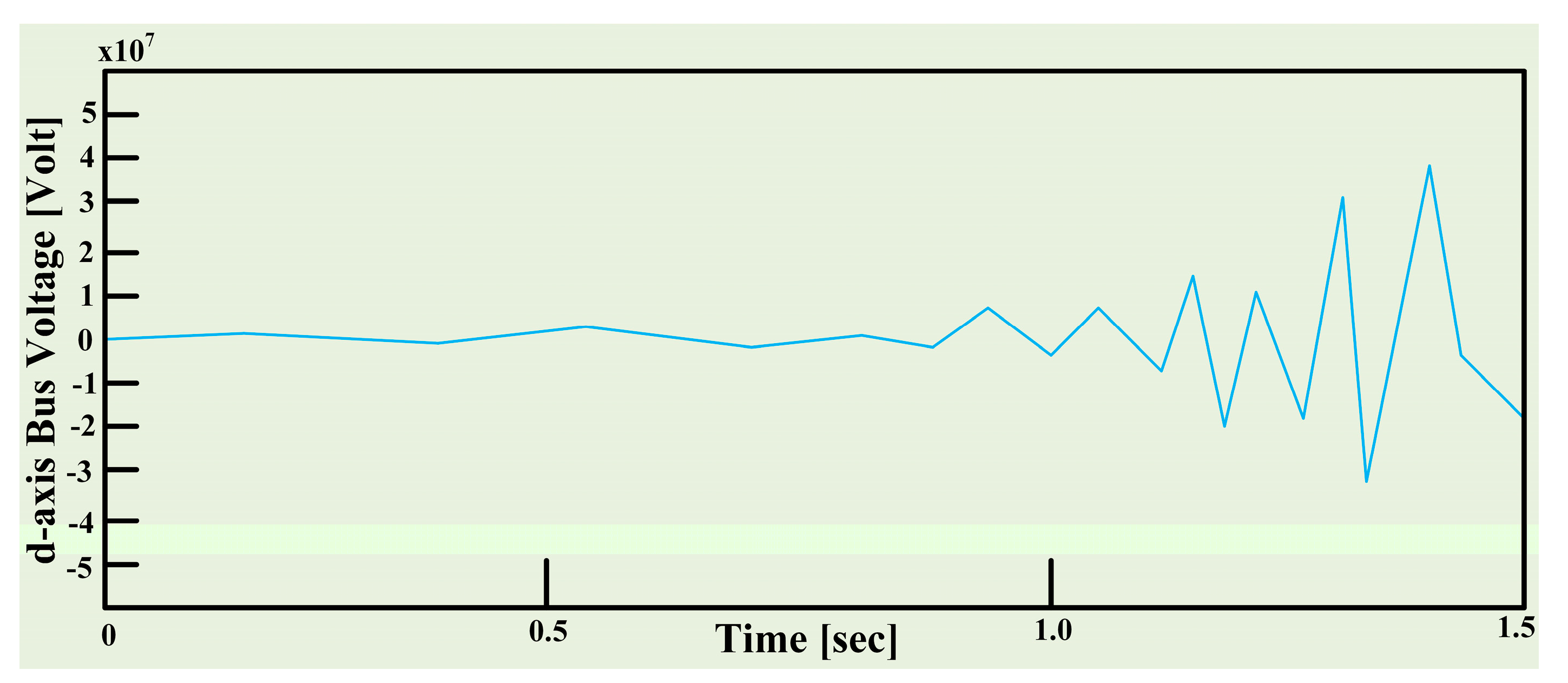
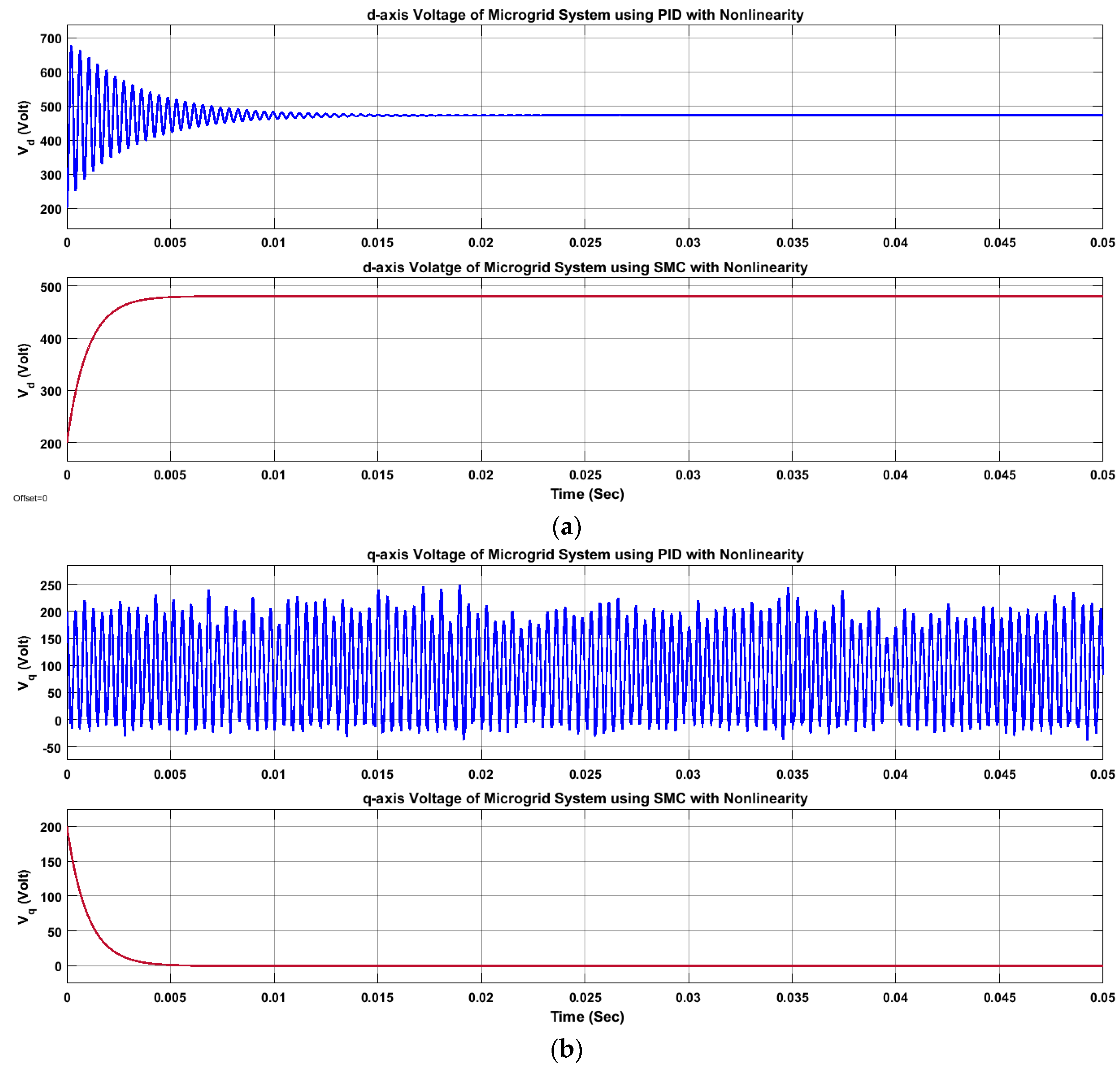
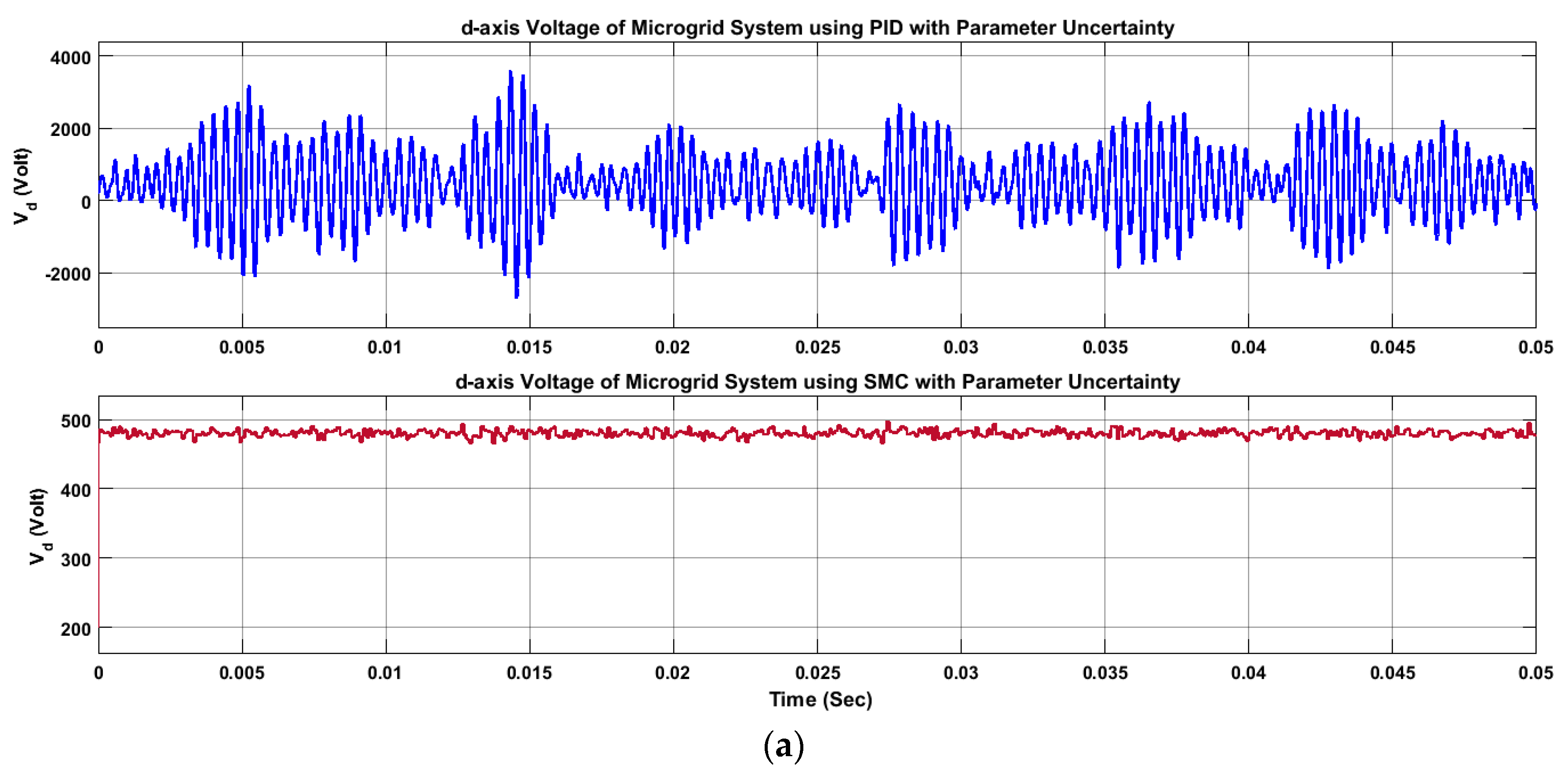
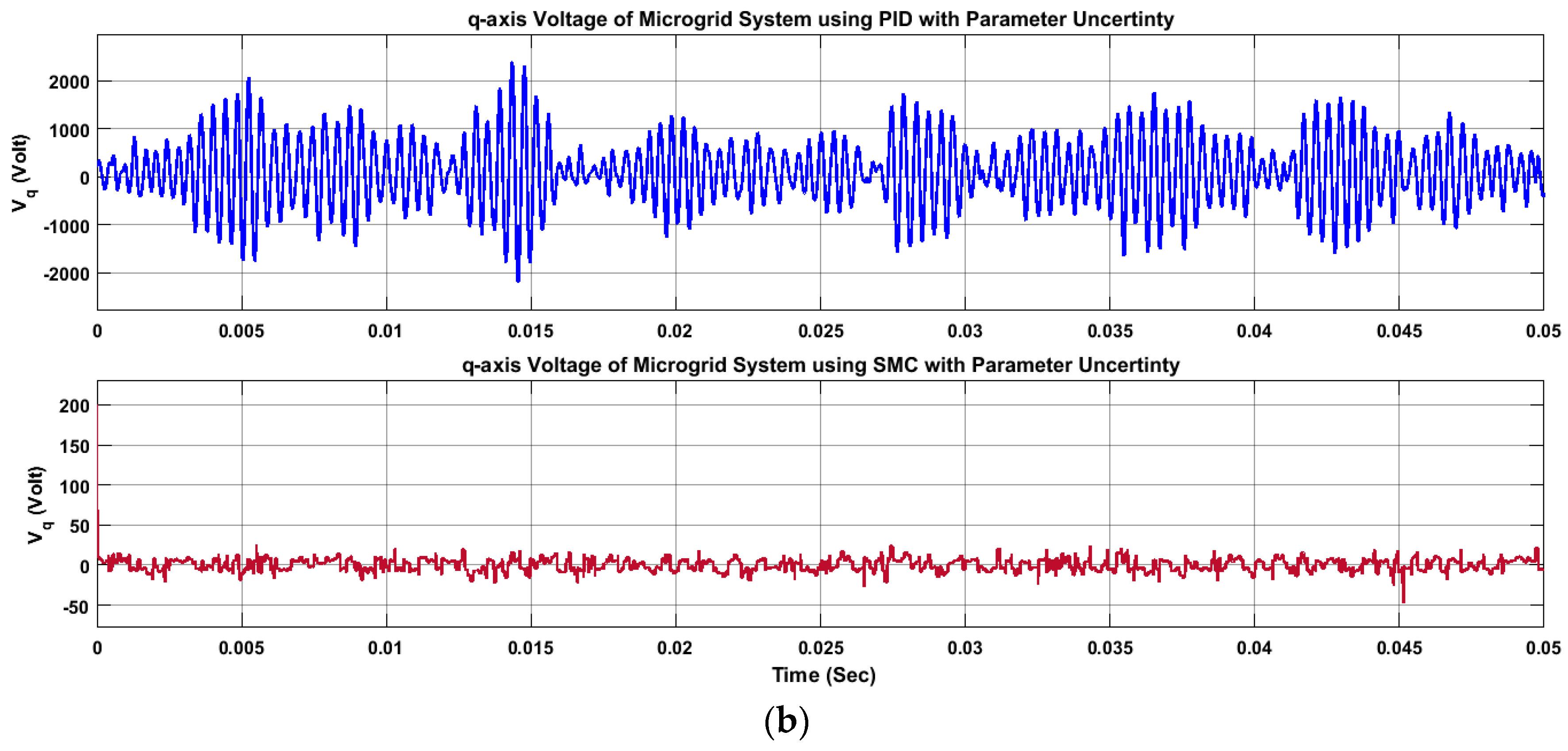
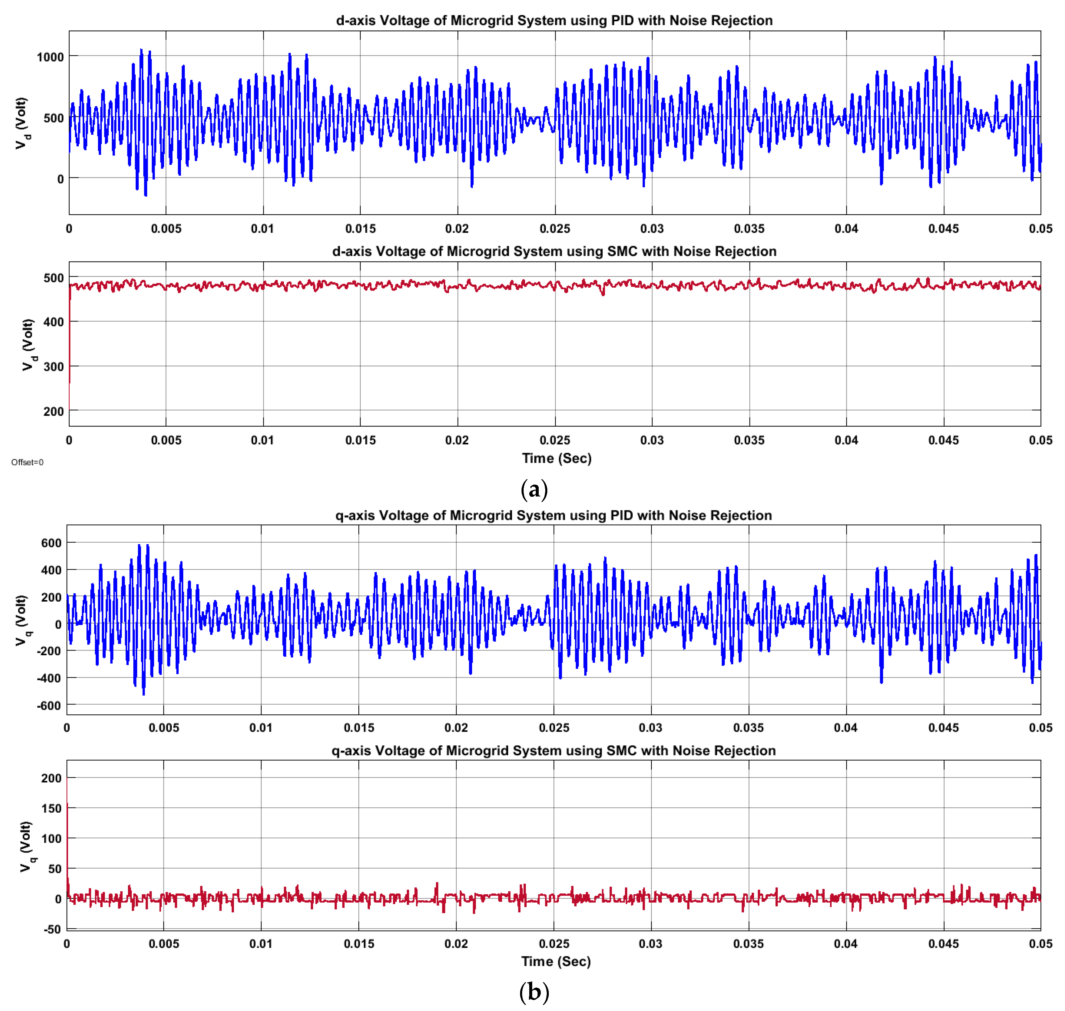
In this section, we will enhance the robustness by introducing the white noise rejection method. From the last section, we can see that we have to measure just two states as all other states are replaced by their bounds. These two parameters are x 3 and x 5 for u 1 and, x 4 and x 6 for u 2 . As we know that multiplicative noise does not affect the stability of the system, we will only consider additive noise. Let, the disturbances added to x 3 , x 4 , x 5 and x 6 be n 3 , n 4 , n 5 and n 6 . Although all the noises; n 3 , n 4 , n 5 and n 6 are white, let their maximum possible value be δ n 3 , δ n 4 , δ n 5 and δ n 6 , respectively.
Using the same method discussed in the last section, let:
e 1   =   ( x 3     x 3 d ) d t ,
e 2   =   e ˙ 1   =   x 3     x 3 d ,
e ˙ 2   =   x ˙ 3     x ˙ 3 d =   f 3 ( x )   +   g 3 ( x ) u 1     x ˙ 3 d ,
Expanding f 3 ( x ) and g 3 ( x ) :
e ˙ 2   =   ω x 4   +   1 c x 1     1 c P 0 x 3     1 c x 5     1 c u 1     x ˙ 3 d ,
Let, the sliding surface be:
s   =   e 1   +   e 2 ,
After differentiating and adding the noises and uncertainties:
s ˙   =   e 2   +   n 3   +   ( ( ω   +   Δ ω ) ( x 4   +   n 4 )   +   1 c ( x ^ 1   +   Δ x 1 )     1 c ( P 0 x 3   +   d P )   1 c ( x 5   +   n 5 )   1 c u 1     x ˙ 3 d ) ,
where d P   =   Δ P /   n 3 and Δ P represents the uncertainties of P 0 . This summarizes the variation on the CPL power term as current. Then we can represent the total parametric uncertainty and noises as:
v d   =   n 3   +   Δ ω n 4   +   Δ ω x 4   +   ω n 4   +   1 c Δ x 1     1 c n 5       1 c d P ;   | | d | |     d m a x ,
where d m a x is the bound of the total disturbance d:
d m a x   = 1 c δ x 1   +   δ n 3   + δ ω δ n 4   +   δ ω δ x 4   +   ω δ n 4   1 c δ n 5   1 c δ P /   δ x 3 ,
Then:
s ˙   =   e 2     1 c x 5     x ˙ 3 d   +   ω x 4   +   1 c x ^ 1     1 c P 0 x 3     1 c u 1   +   d ,
Let this be the Lyapunov candidate function:
V   =   1 2 s 2 ,
  V ˙ =   s   s ˙ =   s ( e 2     1 c x 5     x ˙ 3 d   +   ω x 4   +   1 c x ^ 1     1 c P 0 x 3     1 c u 1   +   d ) ,
We use u 1 :
u 1   =   c [ e 2   +   1 c x 5   +   x ˙ 3 d     ω x 4     1 c x ^ 1   +   1 c P 0 x 3   +   v ] ,
Then, we can obtain:
V ˙ = s ( d + v ) ,
Considering | | d | |     d m a x , the following discontinuous control, v , will make V ˙ to be negative, and consequently, guarantee stability:
v   =   d m a x s a t ( s ε ) ;   ε   >   0 ,
Totally, the control input is:
u 1   =   c [ e 2   +   1 c x 5   +   x ˙ 3 d   +   1 c P 0 x 3     ω x 4     1 c x ^ 1     d m a x s a t ( s ε )   ] ,
Similar analysis is also shown here for u 2 , let:
e 3   =   ( x 4     x 4 d ) dt ,
e 4   =   e ˙ 3   =   x 4     x 4 d ,
e ˙ 4   =   x ˙ 4     x ˙ 4 d   =   f 4 ( x )   +   g 4 ( x ) u 2     x ˙ 4 d ,
Expanding f 4 ( x ) and g 4 ( x ) :
e ˙ 4   =   ω x 3   +   1 c x 2     1 c Q 0 x 4     1 c x 6     1 c u 2     x ˙ 4 d ,
Let, the sliding surface be:
s = e 3 + e 4 ,
After differentiating and adding the noises and uncertainties:
s ˙   =   e 4   +   n 4   +   ( ( ω   +   Δ ω ) ( x 3   +   n 3 )   +   1 c ( x ^ 2   +   Δ x 2 ) 1 c ( Q 0 x 4   +   d Q )   1 c ( x 6   +   n 6 )     1 c u 2     x ˙ 4 d ) ,
where d Q   =   Δ Q /   n 4 And Δ Q   represents the uncertainties of Q 0 . This summarizes the variation on the CPL power term as current. Then we can represent the total parametric uncertainty and noises as:
d   =   n 4     ω n 3     Δ ω n 3     Δ ω x 3   +   1 c Δ x 2     1 c n 6     1 c d Q ;   | | d | |     d m a x ,
where d m a x is the bound of the total disturbance d:
d m a x   =     1 c δ x 2     δ ω δ x 3     δ ω δ n 3     ω δ n 3   +   δ n 4     1 c δ n 6     1 c δ Q /   δ x 4 ,
Then:
s ˙   =   e 3     1 c x 6     x ˙ 4 d   +   ω x 3   +   1 c x ^ 2     1 c Q 0 x 4     1 c u 2   +   d ,
Let this be the Lyapunov candidate function:
V   =   1 2 s 2 ,
V ˙   =   s s ˙   =   s ( e 3     1 c x 6     x ˙ 4 d   +   ω x 3   +   1 c x ^ 2     1 c Q 0 x 4     1 c u 2   +   d ,
We use u 2 :
u 2   =   c [ e 3   +   1 c x 6   +   x ˙ 4 d     ω x 3     1 c x ^ 2   +   1 c Q 0 x 4   +   v ] ,
Then, we can obtain:
V ˙   =   s ( d   +   v ) ,
Considering | | d | |     d m a x , the following discontinuous control, v , will make V ˙ be negative, and consequently, guarantee stability:
v   =   d m a x s a t ( s ε ) ;   ε   >   0 ,
Totally, the control input is:
u 2   =   c [ e 3   +   1 c x 6   +   x ˙ 4 d     ω x 3     1 c x ^ 2   +   1 c Q 0 x 4     d m a x s a t ( s ε ) ,

5. Results

In this paper, a sliding mode controller (SMC) has been selected over a PID controller due to its considerably better performance [39,40,41,42,43,44,45]. In Figure 11, performance comparisons between PID (blue colored) and SMC (red colored) have been shown in the case of: (a) real axis output voltage and (b) reactive axis output voltage for nonlinear system application. It is seen that the PID controller experiences initial chattering rather than stabilized d-axis output voltage in the face of nonlinearity. In the case of the q-axis output voltage, the PID controller doesn’t provide appreciable stabilization, but rather continuous chattering. On the other hand, the sliding mode controller achieved quick and firm output voltage stabilization in the face of microgrid nonlinearity. After that, a performance comparison between PID and SMC is presented at Figure 12 in the case of: (a) real axis output voltage and (b) reactive axis output voltage considering parametric uncertainties. Here, it is evident that the chattering range of the PID controller is considerably more than that of the sliding mode controller. Hence, in the case of parametric uncertainties, SMC shows significantly better performance than the PID controller. Then, in Figure 13, a performance comparison between PID and SMC has been illustrated in the case of: (a) real axis output voltage and (b) reactive axis output voltage considering noise rejection. Here, the SMC handled the instability issue better. Hence, to improve the microgrid stability in the presence of dense CPL, the sliding mode controller is chosen over the PID controller as a load side compensation technique. The algorithm for sliding mode controller simulation platform is presented in Figure 14. In this algorithm, the system is modeled first in state space considering the instabilities caused by intermittency of renewable sources and CPL. If the instability remains within the bounds of a predefined range, no compensation is done. If the predefined boundary is crossed by the instability, the controller is enabled—which decides the amount of real and reactive power required for compensation to make the system stable. This power is then supplied by the energy storage system in terms of active and reactive current through power electronics interface.
Performance comparisons between robustness against parametric variation and robustness analysis against parametric uncertainties, frequency variation and additive Gaussian noise using SMC control technique based on boundary condition are analyzed in Figure 15, Figure 16, Figure 17 and Figure 18. For robustness analysis, we have to take a Lyapunov function and put the feedback system in it. In this case, we will perturb the unknown parameters.
Here, we can also define some numerical values of bounds and the perturbed parameters for robustness analysis:
For u 1
Let, ω   =   60   Hz ,     x 3   =   600   V ,     x 4   =   10   V ,     Δ x 1   =   200   A ,     Δ x 2     =   200   A , n 3   =   50   V ,     n 4   =   50   V   ,     n 5   =   30   A ,     n 6   =   30   A ,     Δ ω   =   10   Hz ,     d P   =   50   A ,     a n d     d Q   =   20   A . Also, we have the numerical value of bounds; δ x 1   =   4000   A , δ x 4   =   100   V , δ ω   =   70   Hz , δ P   =   30   kW , δ Q   =   20   Var ,     δ n 3   =   δ n 4   =   δ n 5   =   δ n 6   =   100   A , ρ x 3   =   200   V , and ε   =   100 . These values represent the parameters of a typical system where ‘ ω ’ represents the frequency, the ‘x’s represent the system voltages and currents, the ‘ Δ x ’s represent the variations in the corresponding system parameters, the ‘n’s represent the noise present in the system, and dP and dQ shows the variation of load in terms of the d and q axis. The rest of the values define the numerical bounds for the perturbed parameters for robustness analysis:
V ˙   =   s ( d   +   v ) =   s ( n 3   +   Δ ω n 4   +   Δ ω x 4   +   ω n 4   +   1 c Δ x 1     1 c n 5     1 c d P     [   1 c δ x 1   +   δ n 3   +     δ ω δ n 4   +   δ ω δ x 4   +   ω δ n 4       1 c δ n 5     δ P C δ x 3 ] s a t ( s ε ) ) ,
V ˙   =   s [ 50   +   ( 10 ) ( 50 )   +   ( 10 ) ( 10 )   +   ( 60 ) ( 50 )   +   1 c ( 200 )     1 c ( 30 )   1 c ( 50 )   [ 1 c 4000   +   100   +   ( 70 ) ( 100 )   +   ( 70 ) ( 100 )   +   ( 65 ) ( 100 )     1 c 100     1 c ( 30000 200 ) ] s a t ( s 100 ) ] ,
V ˙   =   s [ 18.004   ×   10 6     [ 375.021   ×   10 6 ] s a t ( s 100 ) ] ,
Now, if s is either positive or negative, we will get V ˙     0 .
For u 2
V ˙   =   s ( d   +   v )   =   s ( [ n 4     ω n 3     Δ ω n 3     Δ ω x 3   +   1 c Δ x 2     1 c n 6     1 c d Q     [   1 c δ x 2   +     δ n 4     1 c δ n 6     δ ω δ x 3     δ ω δ n 3     ω δ n 3       δ Q /   δ x 4 ] s a t ( s 100 ) ] ,
V ˙   =   s [ 50     ( 60 ) ( 50 )     ( 10 ) ( 600 )     ( 10 ) ( 50 )   +   1 c ( 200 )     1 c ( 30 )   1 c ( 20 )   [ 1 c 1000   +   100     ( 70 ) ( 1000 )     ( 70 ) ( 100 )     ( 65 ) ( 100 )     1 c 100     1 c ( 20 1 ) ] s a t ( s 100 ) ] ,
V ˙   =   s [ 14.99   ×   10 6     [ 79.916   ×   10 6 ] s a t ( s 100 ) ] ,
Now, if s is either positive or negative, we will get V ˙     0 . So, as a derivative of a Lyapunov function is negative, our system will remain stable even in the case of perturbing.

6. Conclusions

Though microgrid systems have several advantages over utility grid systems, to adopt this system for mass electrification is cumbersome due to the CPL instability. To improve the stability scenario of microgrid systems, in this paper, a load side compensation technique has been adopted. Besides a discussion of the previous research work on sliding mode control techniques, a sliding mode controller has been developed for microgrids with constant power loads to assure the control objectives/desired output. Initially, constant power load instability has been presented with necessary examples. After that, the sliding mode control (SMC) technique has been introduced. Apart from that, the control principle of SMC, chattering, chattering reduction, advantages of SMC, controller design, and the control objectives have been delineated with necessary equations and depictions. Then, a robustness analysis of SMC has been presented in this paper. After that, the results and simulations have been illustrated in the case of a number of system parameters between robustness analysis against parametric variation and robustness analysis against parametric uncertainties, frequency variation and additive Gaussian noise using the SMC control technique based on boundary conditions. The algorithm of the proposed system has been presented as well. Later, the performance of the PID and the sliding mode controller have been compared in case of nonlinearity, parameter uncertainties, and noise rejection to justify the selection of the sliding mode controller over the PID controller. To verify the performance of this approach, simulation results have been demonstrated on a virtual platform such as MATLAB/Simulink.

Acknowledgments

No source of funding was provided for this research project.

Author Contributions

All authors were involved equally in the development of the proposed research concept from the basic concept to theoretical prediction and the investigation of the sliding mode controller in microgrids. The numerical simulation software implementation tasks were carried out by Eklas Hossain and Sanjeevikumar Padmanaban, and validated the proposal with the expected outcomes and theoretical background. Ron Perez and Pierluigi Siano shared their expertise in microgrids for validation of the proposal.

Conflicts of Interest

The authors declare no conflict of interest.

References

  1. Hossain, E.; Kabalci, E.; Bayindir, R.; Perez, R. Microgrid testbeds around the world: State of art. Energy Convers. Manag. 2014, 86, 132–153. [Google Scholar] [CrossRef]
  2. Evangelopoulos, V.A.; Georgilakis, P.S.; Hatziargytious, N.D. Optimal operation of smart distribution networks—A review of models, methods and future research. Electr. Power Syst. Res. 2016, 140, 95–106. [Google Scholar] [CrossRef]
  3. Ali Memon, A.; Kauhaniemi, K. A critical review of AC Microgrid protection issues and available solutions. Electr. Power Syst. Res. 2016, 129, 23–31. [Google Scholar] [CrossRef]
  4. Malik, F.H.; Lehtonen, M. A review: Agents in smart grids. Electr. Power Syst. Res. 2016, 131, 71–79. [Google Scholar] [CrossRef]
  5. Papadimitriou, C.N.; Zountouridou, E.I.; Hatziargyriou, N.D. Review of hierarchical control in DC microgrids. Electr. Power Syst. Res. 2015, 122, 159–167. [Google Scholar] [CrossRef]
  6. Sanchez, S.; Ortega, R.; Griño, R.; Bergna, G.; Molinas, M. Conditions for Existence of Equilibria of Systems with Constant Power Loads. IEEE Circuits Syst. I Regul. Pap. 2014, 61, 2204–2211. [Google Scholar] [CrossRef]
  7. Li, Y.; Vannorsdel, K.R.; Zirger, A.J.; Norris, M.; Maksimovic, D. Current Mode Control for Boost Converters with Constant Power Loads. IEEE Trans. Circuits Syst. I Regul. Pap. 2012, 59, 198–206. [Google Scholar] [CrossRef]
  8. Sanchez, S.; Molinas, M. Assessment of a stability analysis tool for constant power loads in DC-grids. In Proceedings of the International Power Electronics and Motion Control Conference (EPE/PEMC), Novi Sad, Serbia, 4–6 September 2012; pp. DS3b.2-1–DS3b.2-5. [Google Scholar]
  9. Barabanov, N.; Ortega, R.; Griñó, R.; Polyak, B. On Existence and Stability of Equilibria of Linear Time-Invariant Systems with Constant Power Loads. IEEE Trans. Circuits Syst. I Regul. Pap. 2016, 63, 114–121. [Google Scholar] [CrossRef]
  10. Trias, A.; Marín, J.L. The Holomorphic Embedding Load flow Method for DC Power Systems and Nonlinear DC Circuits. IEEE Trans. Circuits Syst. I Regul. Pap. 2016, 63, 322–333. [Google Scholar] [CrossRef]
  11. Wu, M.; Lu, D.D.C. A Novel Stabilization Method of LC Input Filter with Constant Power Loads without Load Performance Compromise in DC Microgrids. IEEE Trans. Ind. Electron. 2015, 62, 4552–4562. [Google Scholar] [CrossRef]
  12. Kwasinski, A.; Onwuchekwa, C.N. Dynamic Behavior and Stabilization of DC Microgrids with Instantaneous Constant-Power Loads. IEEE Trans. Power Electron. 2011, 26, 822–834. [Google Scholar] [CrossRef]
  13. Huddy, S.R.; Skufca, J.D. Amplitude Death Solutions for Stabilization of DC Microgrids with Instantaneous Constant-Power Loads. IEEE Trans. Power Electron. 2013, 28, 247–253. [Google Scholar] [CrossRef]
  14. Sanchez, S.; Molinas, M. Large Signal Stability Analysis at the Common Coupling Point of a DC Microgrid: A Grid Impedance Estimation Approach Based on a Recursive Method. IEEE Trans. Energy Convers. 2015, 30, 122–131. [Google Scholar] [CrossRef]
  15. Marx, D.; Magne, P.; Nahid-Mobarakeh, B.; Pierfederici, S.; Davat, B. Large Signal Stability Analysis Tools in DC Power Systems With Constant Power Loads and Variable Power Loads—A Review. IEEE Trans. Power Electron. 2012, 27, 1773–1787. [Google Scholar] [CrossRef]
  16. Magne, P.; Marx, D.; Nahid-Mobarakeh, B.; Pierfederici, S. Large-Signal Stabilization of a DC Link Supplying a Constant Power Load Using a Virtual Capacitor: Impact on the Domain of Attraction. IEEE Trans. Ind. Appl. 2012, 48, 878–887. [Google Scholar] [CrossRef]
  17. Jelani, N.; Molinas, M.; Bolognani, S. Reactive Power Ancillary Service by Constant Power Loads in Distributed AC Systems. IEEE Trans. Power Deliv. 2013, 28, 920–927. [Google Scholar] [CrossRef]
  18. Singh, S.; Fulwani, D.; Kumar, V. Robust sliding-mode control of dc/dc boost converter feeding a constant power load. IEEE Trans. Power Electron. 2015, 8, 1230–1237. [Google Scholar] [CrossRef]
  19. Gautam, A.R.; Singh, S.; Fulwani, D. DC bus voltage regulation in the presence of constant power load using sliding mode controlled dc-dc Bi-directional converter interfaced storage unit. In Proceedings of the IEEE First International Conference on DC Microgrids (ICDCM), Atlanta, GA, USA, 7–10 June 2015; pp. 257–262. [Google Scholar]
  20. Stramosk, V.; Pagano, D.J. Nonlinear control of a bidirectional dc-dc converter operating with boost-type Constant-Power Loads. In Proceedings of the Power Electronics Conference (COBEP), Brazilian, Brazil, 27–31 October 2013; pp. 305–310. [Google Scholar]
  21. Liu, Z.; Liu, J.; Bao, W.; Zhao, Y. Infinity-Norm of Impedance-Based Stability Criterion for Three-Phase AC Distributed Power Systems with Constant Power Loads. IEEE Trans. Power Electron. 2015, 30, 3030–3043. [Google Scholar] [CrossRef]
  22. Jelani, N.; Molinas, M. Asymmetrical Fault Ride Through as Ancillary Service by Constant Power Loads in Grid-Connected Wind Farm. IEEE Trans. Power Electron. 2015, 30, 1704–1713. [Google Scholar] [CrossRef]
  23. Emadi, A. Modeling of power electronic loads in AC distribution systems using the generalized State-space averaging method. IEEE Trans. Ind. Electron. 2004, 51, 992–1000. [Google Scholar] [CrossRef]
  24. Karimipour, D.; Salmasi, F.R. Stability Analysis of AC Microgrids with Constant Power Loads Based on Popov’s Absolute Stability Criterion. IEEE Trans. Circuits Syst. II Express Briefs 2015, 62, 696–700. [Google Scholar] [CrossRef]
  25. Jian, S. Small-signal methods for AC distributed power systems—A review. IEEE Trans. Power Electron. 2009, 24, 2545–2554. [Google Scholar] [CrossRef]
  26. Vilathgamuwa, D.M.; Zhang, X.N.; Jayasinghe, S.D.G.; Bhangu, B.S.; Gajanayake, C.J.; Tseng, K.J. Virtual resistance based active damping solution for constant power instability in AC microgrids. In Proceedings of the IECON 2011—37th Annual Conference on IEEE Industrial Electronics Society, Melbourne, Australia, 7–10 November 2011; pp. 3646–3651. [Google Scholar]
  27. Ganjefar, S.; Sarajchi, M.H.; Mahmoud Hoseini, S. Teleoperation Systems Design Using Singular Perturbation Method and Sliding Mode Controllers. ASME. J. Dyn. Syst. Meas. Control 2017, 136, 051005. [Google Scholar] [CrossRef]
  28. Khalil, H.K. Nonlinear Systems, 3rd ed.; Prentice-Hall: Upper Saddle River, NJ, USA, 2002. [Google Scholar]
  29. Elhalwagy, Y.Z.; Tarbouchi, M. Fuzzy logic sliding mode control for command guidance law design. ISA Trans. 2004, 43, 231–242. [Google Scholar] [CrossRef]
  30. Torchani, B.; Sellami, A.; Garcia, G. Sliding mode control of saturated systems with norm bounded uncertainty. In Proceedings of the 16th IEEE Mediterranean Electrotechnical Conference, Yasmine Hammamet, Tunisia, 25–28 March 2012; pp. 15–18. [Google Scholar]
  31. Sliding Mode Control. Available online: https: //theses.lib.vt.edu/theses/available/etd5440202339731121/unrestricted/CHAP4_DOC.pdf (accessed on 10 May 2017).
  32. Wang, D.; Zhang, Q.; Wang, A. Robust nonlinear control design for ionic polymer metal composite based on sliding mode approach. In Proceedings of the UKACC International Conference on Control (CONTROL), Loughborough, UK, 8–14 July 2014; pp. 519–524. [Google Scholar]
  33. Santi, E.; Li, D.; Monti, A.; Stankovic, A.M. A Geometric Approach to Large-signal Stability of Switching Converters under Sliding Mode Control and Synergetic Control. In Proceedings of the IEEE 36th Power Electronics Specialists Conference, Recife, Brazil, 12–16 June 2005; pp. 1389–1395. [Google Scholar]
  34. Farrell, J.A.; Polycarpou, M.M. Adaptive Approximation Based Control: Unifying Neural, Fuzzy and Traditional Adaptive Approximation Approaches; John Wiley & Sons: Hoboken, NJ, USA, 2006; Volume 48. [Google Scholar]
  35. Bharatiraja, C.; Sanjeevikumar, P.; Siano, P.; Ramesh, K.; Raghu, R. Real Time Foresting of EV Charging Station Scheduling for Smart Energy System. Energies 2017, 10, 377. [Google Scholar]
  36. Ozsoy, E.; Sanjeevikumar, P.; Mihet-Popa, L.; Fedák, V.; Ahmad, F.; Akhtar, R.; Sabanovic, A. Control Strategy for Grid Connected Inverters under Unbalanced Network Conditions—A DOb Based Decoupled Current Approach. Energies 2017, 10, 1067. [Google Scholar] [CrossRef]
  37. Vavilapalli, S.; Sanjeevikumar, P.; Umashankar, S.; Mihet-Popa, L. Power Balancing Control for Grid Energy Storage System in PV Applications—Real Time Digital Simulation Implementation. Energies 2017, 10, 928. [Google Scholar] [CrossRef]
  38. Awasthi, A.; Karthikeyan, V.; Rajasekar, S.; Sanjeevikumar, P.; Siano, P.; Ertas, A.H. Dual Mode Control of Inverter to Integrate Solar-Wind Hybrid fed DC-Grid with Distributed AC grid. In Proceedings of the 16th IEEE International Conference on Environment and Electrical Engineering, Florence, Italy, 7–10 June 2016. [Google Scholar]
  39. Hussain, S.; Alammari, R.; Jafarullah, M.; Iqbal, A.; Sanjeevikumar, P. Optimization Of Hybrid Renewable Energy System Using Iterative Filter Selection Approach. IET Renew. Power Gener. 2017. [Google Scholar] [CrossRef]
  40. Hajizadeh, A.; Norum, L.N.; Hassanzadehc, F.; Sanjeevikumar, P. An Intelligent Power Controller for Hybrid DC Micro Grid Power System. In Lecture Notes in Electrical Engineering; Springer: Berlin, Germany, 2017. [Google Scholar]
  41. Swaminathan, G.; Ramesh, V.; Umashankar, S.; Sanjeevikumar, P. Fuzzy Based Micro Grid Energy Management System using Interleaved Boost Converter and Three Level NPC Inverter with Improved Grid Voltage Quality. In Lecture Notes in Electrical Engineering; Springer: Berlin, Germany, 2017. [Google Scholar]
  42. Swaminathan, G.; Ramesh, V.; Umashankar, S.; Sanjeevikumar, P. Investigations of Microgrid Stability and Optimum Power sharing using Robust Control of grid tie PV Inverter. In Lecture Notes in Electrical Engineering; Springer: Berlin, Germany, 2017. [Google Scholar]
  43. Samee, S.; Khan, S.; Vengatesan, K.; Bhaskar, M.S.; Sanjeevikumar, P.; Jaspreetkuar, P. Smart City Automatic Garbage Collecting System for a Better Tomorrow. In Lecture Notes in Electrical Engineering; Springer: Berlin, Germany, 2017. [Google Scholar]
  44. Tiwaria, R.; Ramesh Babu, N.; Sanjeevikumar, P. A Review on GRID CODES—Reactive power management in power grids for Doubly-Fed Induction Generator in Wind Power application. In Lecture Notes in Electrical Engineering; Springer: Berlin, Germany, 2017. [Google Scholar]
  45. Tiwari, R.; Ramesh Babu, N.; Arunkrishna, R.; Sanjeevikumar, P. Comparison between PI controller and Fuzzy logic based control strategies for harmonic reduction in Grid integrated Wind energy conversion system. In Lecture Notes in Electrical Engineering; Springer: Berlin, Germany, 2017. [Google Scholar]
Figure 1. Typical V-I characteristics of (a) Constant Voltage Load (CVL); (b) Constant Power Load [3].
Energies 10 01086 g001
Figure 2. Equivalent circuit of an AC microgrid with CPL and CVL [26].
Energies 10 01086 g002
Figure 3. d-q axis model of a microgrid system. (a) d-axis model of a microgrid; (b) q-axis model of a microgrid.
Energies 10 01086 g003
Figure 4. d-axis bus voltage instability due to CPL.
Energies 10 01086 g004
Figure 5. q-axis bus voltage instability due to CPL.
Energies 10 01086 g005
Figure 6. The schematic diagram of a microgrid system, which has been made unstable by a CPL while control inputs are absent. Equivalent circuits and bus voltages of the microgrid are shown for d-axis in (a), and for q-axis in (b); the measurement locations are also indicated.
Energies 10 01086 g006
Figure 7. d-axis model of the load side real power compensation method.
Energies 10 01086 g007
Figure 8. q-axis model of the load side reactive power compensation method.
Energies 10 01086 g008
Figure 9. Schematic representation of sliding mode control scheme [28].
Energies 10 01086 g009
Figure 10. Chattering as a result of imperfect control switching [31].
Energies 10 01086 g010
Figure 11. Performance comparison between PID (blue colored) and SMC (red colored) in the case of (a) real axis output voltage (Vd) and (b) reactive axis output voltage (Vq) for nonlinear system application.
Energies 10 01086 g011
Figure 12. Performance comparison between PID (blue colored) and SMC (red colored) in the case of (a) real axis output voltage (Vd) and (b) reactive axis output voltage (Vq) considering parametric uncertainties.
Energies 10 01086 g012aEnergies 10 01086 g012b
Figure 13. Performance comparison between PID (blue colored) and SMC (red colored) in the case of (a) real axis output voltage (Vd) and (b) reactive axis output voltage (Vq) considering noise rejection.
Energies 10 01086 g013
Figure 14. Algorithm for sliding mode control of a microgrid with CPL.
Energies 10 01086 g014
Figure 15. (a) d-axis current comparison; (b) q-axis current comparison, between robustness analysis against parametric variation and robustness analysis against parametric uncertainties, frequency variation and additive Gaussian noise using SMC control technique based on boundary conditions.
Energies 10 01086 g015aEnergies 10 01086 g015b
Figure 16. (a) d-axis bus voltage comparison; (b) q-axis bus voltage comparison, between robustness analysis against parametric variation and robustness analysis against parametric uncertainties, frequency variation and additive Gaussian noise using SMC control technique based on boundary conditions.
Energies 10 01086 g016
Figure 17. (a) d-axis current (CVL load) comparison; (b) q-axis current (CVL load) comparison, between robustness analysis against parametric variation and robustness analysis against parametric uncertainties, frequency variation and additive Gaussian noise using SMC control technique based on boundary condition.
Energies 10 01086 g017
Figure 18. (a) d-axis current compensation (d-axis control signal) comparison; and (b) q-axis current compensation (q-axis control signal) comparison, between robustness analysis against parametric variation and robustness analysis against parametric uncertainties, frequency variation and additive Gaussian noise using SMC control technique based on boundary condition.
Energies 10 01086 g018aEnergies 10 01086 g018b

