Optimal Dynamic Analysis of Electrical/Electronic Components in Wind Turbines
by
 ,
,
Fausto Pedro García Márquez
1,* ,
,
Alberto Pliego Marugán
1, 
Jesús María Pinar Pérez
2,
Stuart Hillmansen
3 and 
Mayorkinos Papaelias
4 1
Ingenium Research Group, Universidad Castilla-La Mancha, 13071 Ciudad Real, Spain
2
CUNEF-Ingenium, University College of Financial Studies, 28040 Madrid, Spain
3
School of Electronic, Electrical & Computer Engineering, University of Birmingham, Birmingham B15 2TT, UK
4
School of Metallurgy and Materials, University of Birmingham, Birmingham B15 2TT, UK
*
Author to whom correspondence should be addressed.
Energies 2017, 10(8), 1111; https://doi.org/10.3390/en10081111
Submission received: 23 May 2017
/
Revised: 28 June 2017
/
Accepted: 18 July 2017
/
Published: 31 July 2017
(This article belongs to the Collection Wind Turbines)
Abstract
:Electrical and electronic components are very important subcomponents in modern industrial wind turbines. Complex multimegawatt wind turbines are continuously being installed both onshore and offshore, continuously increasing the demand for sophisticated electronic and electrical components. In this work, most critical electrical and electronic components in industrial wind turbines have been identified and the applicability of appropriate condition monitoring processes simulated. A fault tree dynamic analysis has been carried out by binary decision diagrams to obtain the system failure probability over time and using different time increments to evaluate the system. This analysis allows critical electrical and electronic components of the converters to be identified in different conditions. The results can be used to develop a scheduled maintenance that improves the decision making and reduces the maintenance costs.
1. Introduction
The environmental benefits arising from the use of wind energy, together with energy policies, mean that the total installed capacity increases every year worldwide. The availability of installed wind turbines (WTs) must be improved to enhance productivity and maximize benefits.
The total global installed wind energy capacity was 486 GW by the end of 2016 [1]. The Global Wind Energy Council (GWEC) forecast anticipates that the cumulative global installed wind energy capacity will be over 800 GW by the end of 2021. Wind energy is expected to continue growing until at least 2050. For a 20-year lifetime, the operation and maintenance (O&M) costs of 750 kW turbines is about 25–30% of the overall energy generation cost, or 75–90% of the investment costs over the life of the wind turbine. Therefore, it is essential to improve the availability, reliability and operational lifetime of WTs to make this energy more efficient [2].
The O&M costs for 2 MW turbines might be 12% less than an equivalent project of 750 kW WTs [3]. The increasing size of the WTs has led to the development of sophisticated maintenance strategies to avoid loss of production [4]. Figure 1 suggests that the largest WTs fail more frequently and, therefore, require more maintenance [5].
Certain WT components fail earlier than expected, causing unscheduled downtimes that can be expensive [6]. Condition monitoring systems (CMS) [7,8] are extensively employed to improve the WT availability and reduce the O&M costs. However, there is a degree of uncertainty about the appropriateness of applying specific maintenance policies to the components of a WT [9].
Figure 2 [10] illustrates the major components of most installed WTs. Driven by the wind, the blades and rotor transmit mechanical energy to the generator, being the low speed shaft supported by the mean bearings. The gearbox monitors the generator speed so that optimal electricity is generated. The nacelle, and hence rotor alignment with respect to the direction of the wind, is controlled by the yaw system at the top of the tower.
The configuration of the WT presented in Figure 2 has an indirect drive system because it employs a gearbox to increase the rotational speed of the shaft that drives the generator. The direct drive configuration does not use a gearbox, but it needs different generators and electric power converters to adapt the energy to the grid frequency.
The main generators used in WTs are squirrel-cage induction generator, wound rotor induction generator, doubly-fed induction generator, permanent magnet synchronous generator (PMSG) and electrically excited synchronous generator [11]. Direct drive configurations use larger and more expensive generators (heavier and multi-pole) than indirect drive types.
Hansen et al. [12,13] identify four types of WT configuration (A, B, C and D), which may be classified together with the sub-types given by Li and Chen [14]. This classification and the main characteristic of each configuration are shown below:
- Type A: Constant speed.
- -
- A0: WTs use passive stall control;
- -
- A1: WTs employ active stall control;
- -
- A2: WTs use a pitch control system, the most advanced technology used in larger WTs;
- Type B: Limited variable speed;
- Type C: Variable speed with partial-scale frequency converter. With DFIG (doubly fed induction generator);
- Type D: Variable speed with full-scale frequency converter:
- -
- DD: Direct-drive: Gearless and variable speed with full-scale frequency converter:
- o
- DDE: This type uses an electrically excited synchronous generator.
- o
- DDP: This group uses a permanent magnet synchronous generator, PMSG;
- -
- DI: Indirect-drive: Variable speed indirect drive with a full-scale power converter:
- o
- DI1P: It is the only configuration with a single-stage gearbox with PMSG;
- o
- DI3W: Three stages gearbox with a wound rotor synchronous generator;
- o
- DI3P: Three stages gearbox with PMSG;
- o
- DI3S: Three stages gearbox with squirrel-cage induction generator.
Figure 3 shows the component cost distribution for a typical 2 MW WT such as the WT shown in Figure 2. Note that the electrical and electronic components account for a considerable percentage, which increases for those configurations with a greater use of electronics such as direct drive WTs.
Some failures, such as leaking and corrosion, can be detected by visual inspection. The noise coming from the bearings can also indicate physical condition [16,17]. However, many typical failures, e.g., electric short circuits in the generator and converters, demand more sophisticated maintenance.
The cost per failure increases due to the cost of corrective maintenance and the loss of production during downtimes. A proper CMS can be used to detect more faults. Early detection of incipient faults prevents major component failures and allows predictive strategies to be carried out [18,19,20]. The capability of a CMS depends on the number and type of sensors, and signal processing [21,22,23,24,25]. It involves measuring, e.g., current, voltage, temperature, humidity, etc., and turning them into electric signals to be processed and monitored. It requires sensors and measurements to carry out basic operations, e.g., amplification, filtering, linearization, modulation/demodulation, etc. Optimization techniques may be employed [26] in the processing of the signals by a digital signal processor. The most common signal processing methods employed in a supervisory control and data acquisition system (SCADA) are:
- Statistical methods.
- Trend analysis.
- Filtering methods.
- Time-domain analysis.
- Cepstrum analysis.
- Time synchronous averaging
- Fast-Fourier transform.
- Amplitude demodulation.
- Order analysis.
- Wavelet transforms.
- Hidden Markov models.
- Novel approaches.
This paper presents a novel approach that uses the data provided by the CMS to analyze the converters and main electrical components of any WT. The results will support the optimization of CMS design and investment. The approach employs fault trees (FTs) and binary decision diagrams (BDDs) for an efficient determination of the system failure probability over time. Additionally, different importance measures (IMs) have been considered to identify the events that contribute more to this probability. Finally, a FT has been developed and analyzed qualitatively and quantitatively considering a large number of research studies. The main components of the converters and electrical parts of the WTs have been considered according to the advice of industrial experts involved in the European NIMO [27] and OPTIMUS [28] projects. Finally, the critical components have been set in different scenarios and the fault probabilities of the events, which would be given by the CMS in real conditions, have been simulated.
2. Electrical/Electronic Failures Analysis
Figure 4 shows the annual failure probabilities of the main components of a WT. The maximum, minimum and median values are shown for each component from different estimations [29]. The figure illustrates that the components with the highest failure probability are the electronics, being more than double that estimated for the rest of the components. Therefore, the electrical and electronic components must be considered in detail.
The literature collects different critical failures for the generator [30,31,32,33,34,35], and for the power electronics and electric controls failure [30,34,36]. Figure 5 shows the failure root distribution in power electronic systems [37].
A study of failure modes and effects for WTs in 2010 (from the RELIAWIND project [38]) noted the causes of failure and failure modes of a specific 2 MW WT with a diameter of 80 m [39]. Some causes of electrical failures are:
- Calibration error
- Connection failure
- Electrical overload
- Electrical short
- Insulation failure
- Lightning strike
- Loss of power input
- Conducting debris
- Software design fault
- Electrical insulation
- Electrical failure
- Output inaccuracy
- Software fault
- Intermittent output
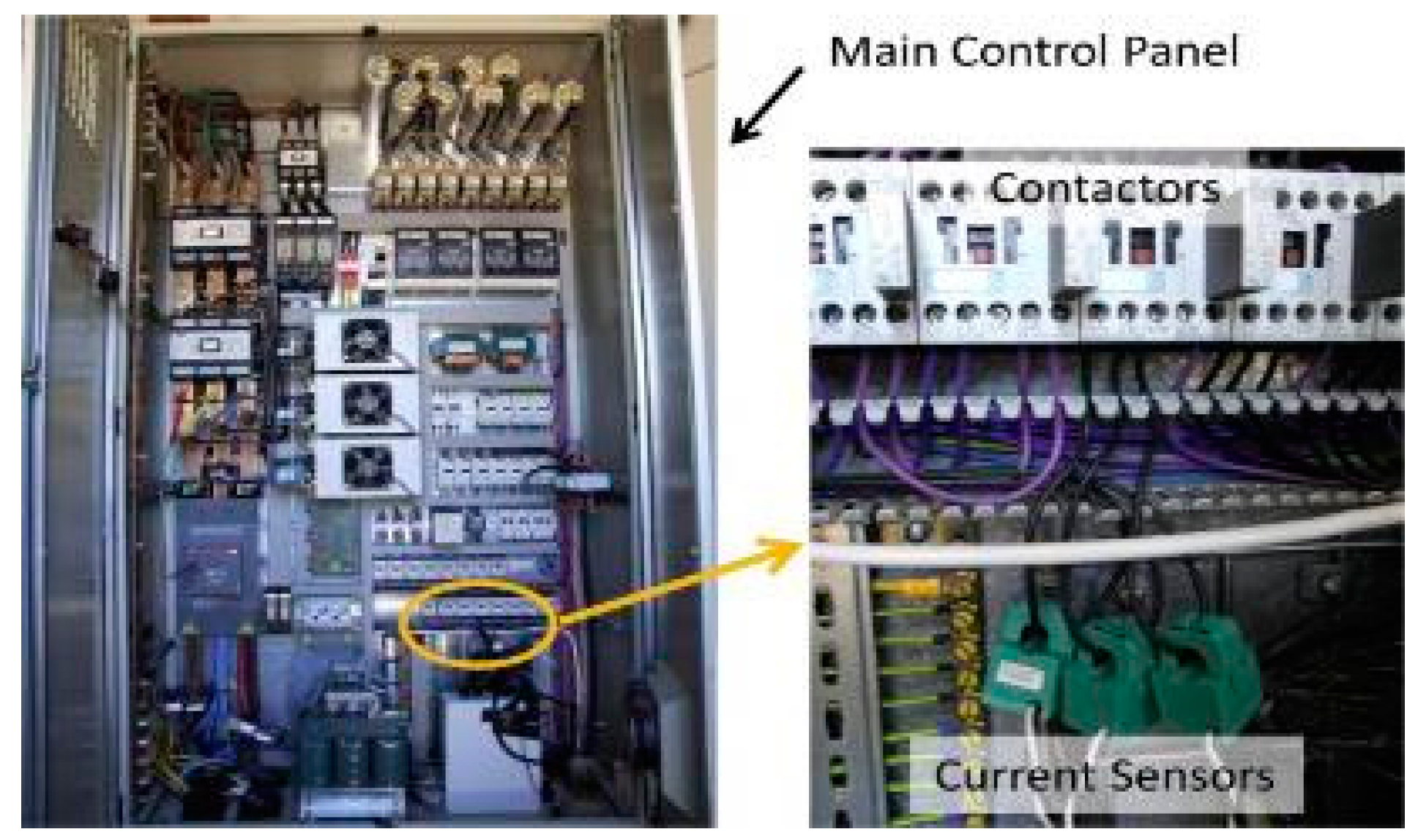
The reliability analysis requires information about each cause of failure. For this purpose, CM of electrical equipment such as converters, motors, generators and accumulators, is typically performed using voltage and current analysis (see Figure 6). Discharge measurements are used for medium and high voltage grids. A spectral analysis of the stator current in the generator can be used for detecting isolation faults in the cabling without influencing WT operation [41].
Electrical resistance is also used for the structural evaluation of certain WT components. It varies with stiffness, and abrupt changes can be used to detect cracks, delamination, and fatigue. Hence, the technique can be applied on in-service WTs. The resistance principle is useful for detecting fatigue damages as demonstrated in [43]. These techniques are identified as research-related activities, but there is significant potential in applying them successfully in real case studies.
Thermography is usually used for monitoring electronic and electrical components and identifying failures [44]. This technique is only applied off-line, and often involves visual interpretation of hot spots that arise due to a bad contact or a system failure, but new cameras and diagnostic software are becoming available for on-line monitoring processes. Infrared cameras [45] have been used to visualize temperature variations in the surface of the blades [46] and can “effectively indicate cracks as well as places threatened by damage” [47]. The converter configuration is essential for the reliability analysis, being the most common [48]: Diode rectifier-Boost-Pulse Width Modulation (PWM) inverter, Two-Level Back-To-Back (2L-BTB) voltage source converter, Three-Level Neutral-Point diode Clamped Back-To-Back (3L-NPC-BTB), multicell converters with 2L-BTB or Power Feed Equipment (PFE) module.
Most of the research studies in the literature propose algorithms to control the specific components and configurations of WTs. For instance, Alrifai et al. [49] proposed a feedback linearization controller for a DFIG with a 3L-NPC-BTB. Xu et al. [50] proposed a slip control strategy to regulate a PWM converter to control the output power. Xiao et al. [51] developed a fuzzy based strategy for controlling DFIG and review many control techniques for different converter configurations.
The authors have not found any previous research work that analyses all the components together from the point of view of reliability. A new approach is proposed that will analyse the main electrical and electronic components. It is important to note that they could be simplified or extended, but in this research study the authors have considered in this research study a certain set of events, following the opinion of the experts [27,28].
3. Reliability Analysis
FT is a tool for analyzing a system composed of several events. FT provides an alternative method to represent a system, including the logical interrelations between the components. Logical operators “AND” and “OR”, together with the events (or components), will allow a better perception of the system.
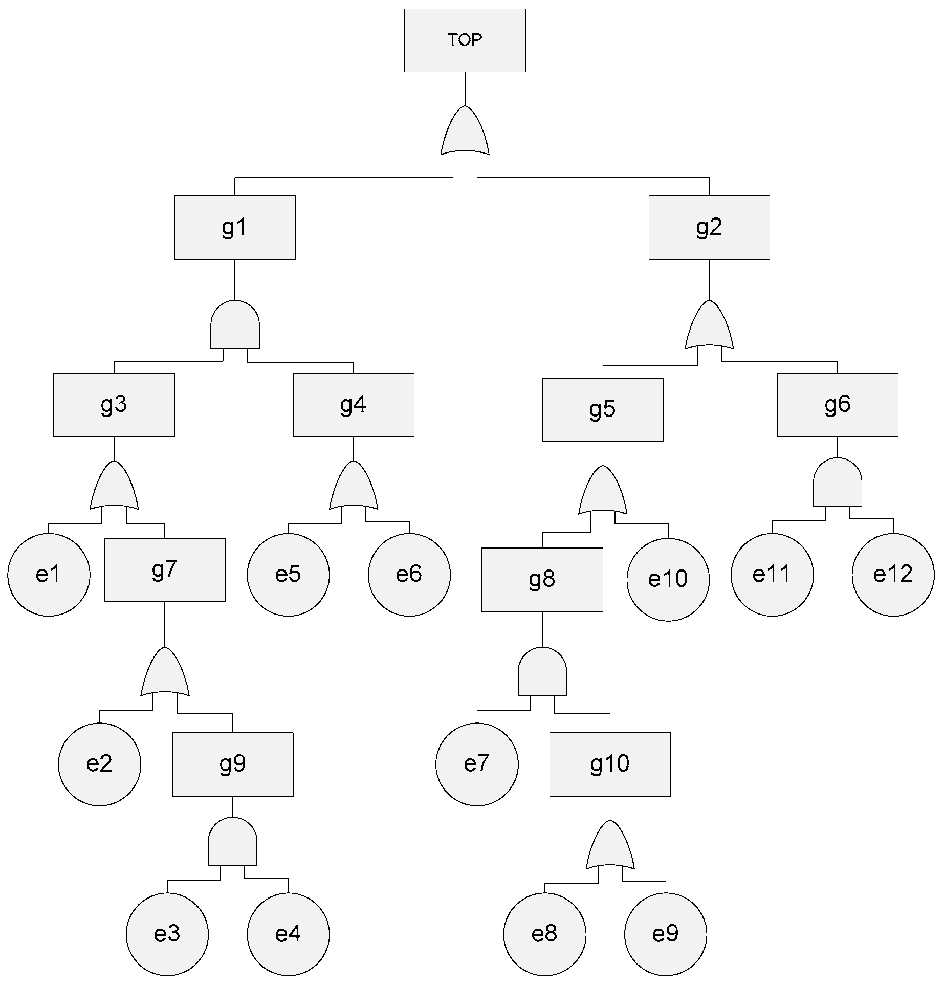
Figure 7 shows a FT composed by 12 basic events (ei) and 10 non-basic events (gi). An event is called a “basic event” if it cannot be broken down into simpler components. They are connected by logical gates. The example shown in Figure 7 has seven “OR” gates and four “AND” gates. Top event is an undesirable event and it is unique in the FT. Non-basic events can be repeated in the FT, but their branch must be the same. FTs provide the information required to carry out a qualitative analysis. BDDs have been successfully found in the constant search for an efficient way to simulate FTs. BDD is a direct graph representation of a Boolean function where equivalent Boolean sub-expressions are uniquely represented [52].
Further information about the origins of BDDs can be found in references [53,54]. The main data provided by BDD are the Cut-Sets (CS). A CS is a path of the BDD “from the top to a one” that provides the combination of events that would cause a system failure.
The number of CSs (BDD size) and the computational cost have a strong dependence on the basic events ordering [55]. Different ranking methods can be used to reduce the number of CS, and consequently, to reduce the computational runtime. There is not a unique method that can provide the best solution in all cases. In this paper, the “Level”, “Top-down-Left-Right” (TDLR), “AND”, “Depth First Search” (DFS) and “Breadth-First Search” (BFS) methods [56] are considered for listing the events, and a comparative analysis is done in order to set the best ranking order. The order of the events will not modify the probability of the top event in any case, i.e., different orders will provide equivalent BDDs.
The TDLR method generates a ranking of the events by ordering them from the original FT structure in a top-down and then left-right manner [57]. The listing of the events is initialized, at each level, in a left to right path adding the basic events found in the ordering list. If any event has been considered and located previously, then this event must not be considered.
The DFS approach goes from top to down of a root and each sub-tree from left to right. This procedure is a non-recursive implementation and all freshly expanded nodes are added as last-input last-output process [58].
The BFS algorithm begins ordering all the basic events obtained expanding from the standpoint by the first-input first-output procedure. The events not considered are added in a queue list named “open”. The list will be recalled “closed” list when every event is studied [59].
The “level” method creates a ranking regarding to the level of the events. The level of any event corresponds to the number of the gates from that event to the top event. Should two or more events have the same level, the event that appears early in the tree will have highest priority [60].
The “AND” criterion sets that the importance of the basic event is based on “AND” gates located between the k event and the top event. These gates imply redundancies in the systems [61]. Basic events with the highest number of “AND” gates will be ranked at the end. In the case of duplicated basic events, the event with less “AND” gates has priority. Finally, basic events with the same number of “AND” gates can be ranked as the TDLR method approach. Table 1 shows the number of CSs obtained by doing the conversion in Figure 7 with the five different ranking methods mentioned above.
The following expressions correspond to the first four CSs out of 31 obtained with DFS method, which is the best one for converting the FT in Figure 7:
The unavailability of the system () can be achieved because the CSs are mutually exclusive, and it is expressed as the sum of probabilities of all the CSs. This expression will represent the unavailability function of the system. It is defined as:
where n corresponds to the total number of CSs. Therefore, Qsys = P(CS1) + P(CS2) + P(CS3) + P(CS4) + … = P(e5)·P(e1) + P(e6)·(1 − P(e5))·P(e1) + P(e10)·(1 − P(e6))·(1 − P(e5))·P(e1) + P(e8)·P(e7)·(1 − P(e10))·(1 − P(e6))·(1 − P(e5))·P(e1) + …
The nature of the events considered in the FT could be different, but a probability assignment is necessary to obtain the system failure probability. Unfortunately, the literature does not include the values of these probabilities over time, and the WT operators are reluctant to provide them. Therefore, the following time–dependent functions have been considered to estimate the probability of each event . In this paper, the time units correspond to ‘months’.
I Constant probability.
The probability of the event is constant
where K is a constant value from 0 to 1.
II Exponential increasing probability.
The probability function assigned is , where is a parameter that has only positive values and determines the rising velocity of the probability.
III Linear increasing probability
where m determines the rising velocity of the probability.
IV Periodic probability
The events have a periodic behaviour, according to the following expression:
where is a parameter that is positive and determines the rising velocity of the probability and is a parameter that determines the period size.
Once the has been obtained over time, it is essential to identify the events that are most important at each time. For this purpose, the IMs can be used to evaluate the contribution of each event to the global system unavailability. In this research, three heuristic IMs (Birnbaum, Criticality, and Fussell-Vesely) based on the probability of each component k to cause a system failure [62] are calculated.
4. FT Dynamic Analysis for Converter, Generator, Electrical and Electronic Components
The approach presented in this work has been employed to analyse the generator, electrical and electronic components that are installed inside the nacelle. The high-speed shaft drives the rotational torque to the generator, where the mechanical energy is converted to electrical energy. This conversion needs a specific input speed, or a power electronic equipment to adapt the output energy from the generator to the requirement of the grid. Several authors have studied the faults related to converters and proposed methods to detect and prevent them. For instance, Swain and Ray [65] proposed the analysis of short circuit fault for a DFIG with active crowbar protection; Qiu et al. studied open-circuit fault features and proposed a new fault diagnosis algorithm to accurately detect faulted IGBT in the circuit arms of WT converters [66]. De Moura et al. [67] proposed a classification of imbalance levels based on the analysis of vibration signal. Faiz and Moosavi [68] developed a method for detecting air gap and other kinds of eccentricities.
To summarize, faults in generators can be the result of electrical or mechanical causes [32]. The main electrical faults are due to open-circuits or short-circuits in the rotor or stator [30] that could cause overheating [69]. Previous research work has demonstrated that bearings, rotors and stators involve a high failure rate in WTs [35]. The bearings failures of the generator are usually caused by cracks, asymmetry and imbalance [70]. The rotor and stator failures can be caused by broken bars [33], air-gap eccentricities and dynamic eccentricities, among other failures [30]. Rotor imbalance and aerodynamic asymmetry can be generated by the non-uniform accumulation of ice and dirt over the blade systems [30]. Table 2 lists the main elements and failures in the generator, electrical and electronic components [71].
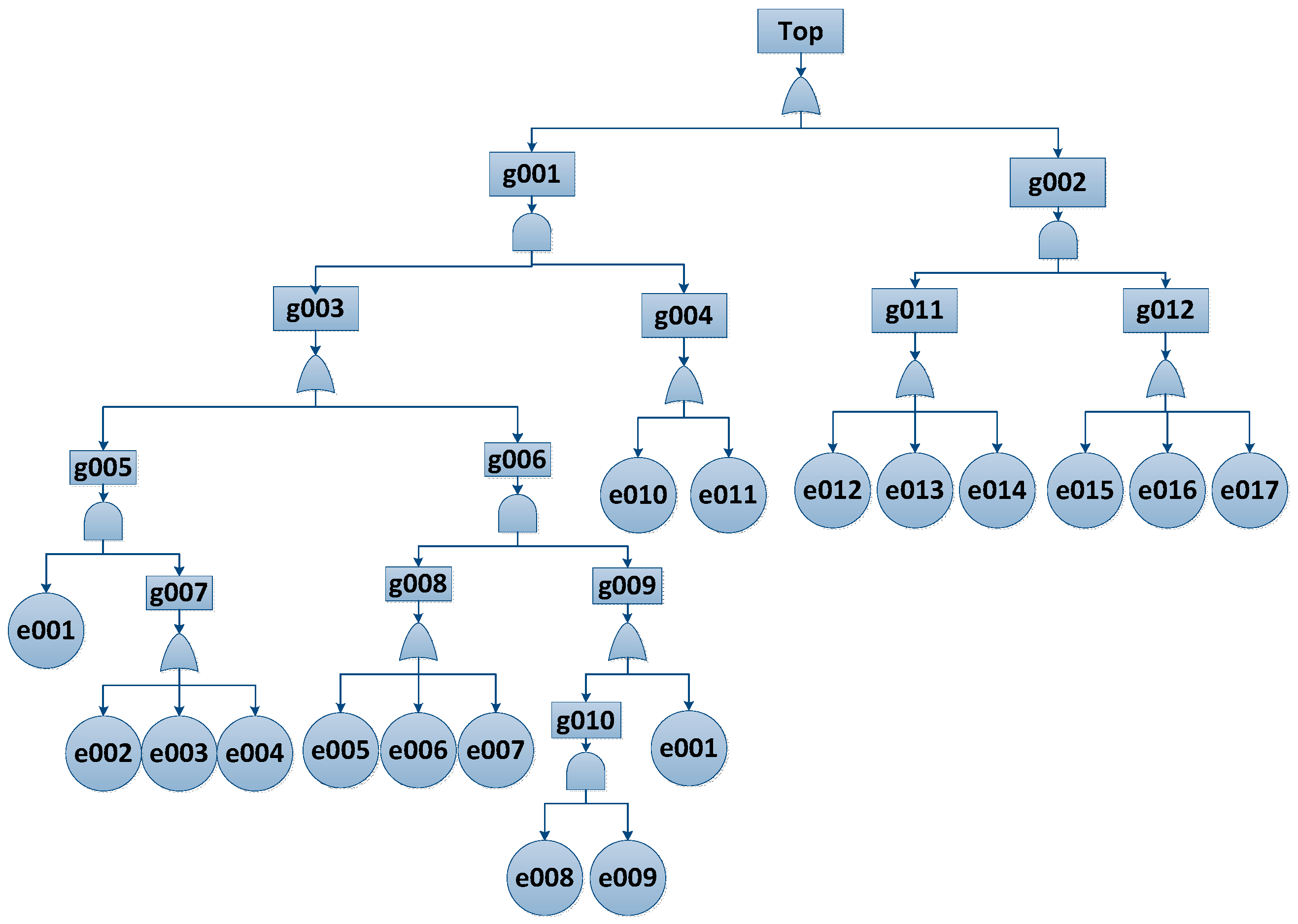
Figure 8 presents the FT for the main elements of the converter, generator, electrical and electronic components given in Table 2.
The FT is solved by BDDs, based on the method described in Section 2 and using different ordering methods. Table 3 shows the number of CSs provided by each method. The AND, TDLR and Level methods provide the minimum number of CSs, 99, whereas the DFS and BFS methods get 171 CSs.
A probability assignment has been done by using the time-dependent functions defined in Section 3.
Table 4 shows the parameters that define the probability of each event over time. The parameters have been set according to the experience of different partners from the NIMO [27] and OPTIMUS FP7 European projects [28]. For confidentiality reasons, there is no detailed information of the specific components or WTs. The main purpose in this study is to show an example close to reality. This numerical dataset has been arbitrarily generated for each event by simulations.
The probability functions that link Table 2 and Table 4 have been chosen by the authors considering the engineering interpretation of each event. For instance, the event “e008” (Rotor and stator fault) shows a constant probability of occurrence over time and the “e014” (gate driven circuit) shows a linear increasing probability, i.e., the contribution to the system failure of the first event does not change over time but the contribution of the second event continues to rise until the probability is 1; the event “e016” (Dirty) has been related to a periodic probability because the dirty is expected to be eliminated during maintenance processes; the event 017 (terminal damage) is considered as linear increasing probability because the responsible phenomena, such as wear or fatigue, increase over time. The use of dynamic probabilities for the events enables system failure probability to be determined over time.
Figure 9 shows the probability assigned to each event. The events have different behaviors according to the values of their parameters. The time units considered in this paper correspond to months.
Figure 10 presents Qsys(t) over time. This probability has been obtained for 20 months. It does not continue rise because there are events (periodic functions) that undergo preventive maintenance.
The system failure probability must be below the failure probability threshold. The maintenance tasks should be set and carried out when the system is close to this threshold.
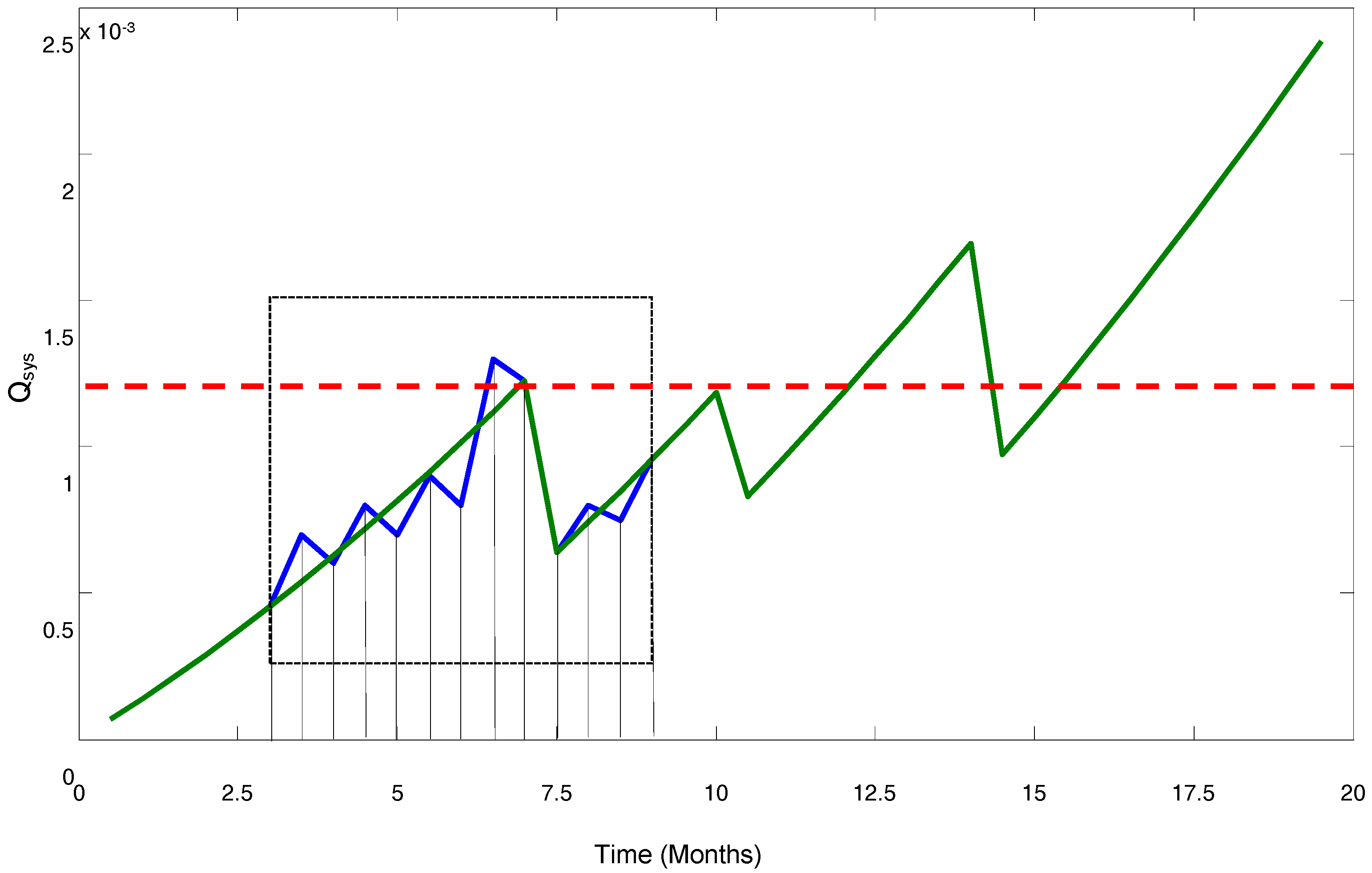
The approach proposed in this paper allows the Qsys to be obtained over time using different time increments to evaluate the system. This is a novelty regarding the state of the art that has resulted in increasing the accuracy of the quantitative analysis. Figure 11 shows the Qsys obtained by using a variable time increment from 3 to 9 (blue line). The time increment is five times smaller than the increment used from 9 to 20 (green line). This is an important advantage because the critical zone (marked as dashed square) can be analysed in further detail. A threshold has been arbitrarily established with probability of 0.00125 (horizontal red dashed line).
Figure 11 shows that the accuracy in the critical zone is greater. This allows detailed analysis the moment the failure probability exceeds the threshold. This procedure shows that the threshold is exceeded in the seventh month, however, in Figure 10 the threshold is not exceeded until the mid-twelfth month. This is an illustrative example about the flexibility of the method and its accuracy in critical zones [72].
IMs have been calculated employing the methods Birnbaum (Figure 12), Criticality (Figure 13), and Fussel-Vesely (Figure 14), described in Section 3 and applied to the FT shown in Figure 8. The Birnbaum’s measures are similar for events e001 to e011, whereas e012, e013 and e014 are identified as the most critical, followed by e015, e016 and e017 (see Figure 10). According to these results, short, open and gate driven circuits are the most critical events due to their occurrences will cause a global system failure. Although the probabilities of these events have been considered as constant or linear increased, their Birnbaum importance is not constant but it is highly influenced by the “health” of the rest of the components.
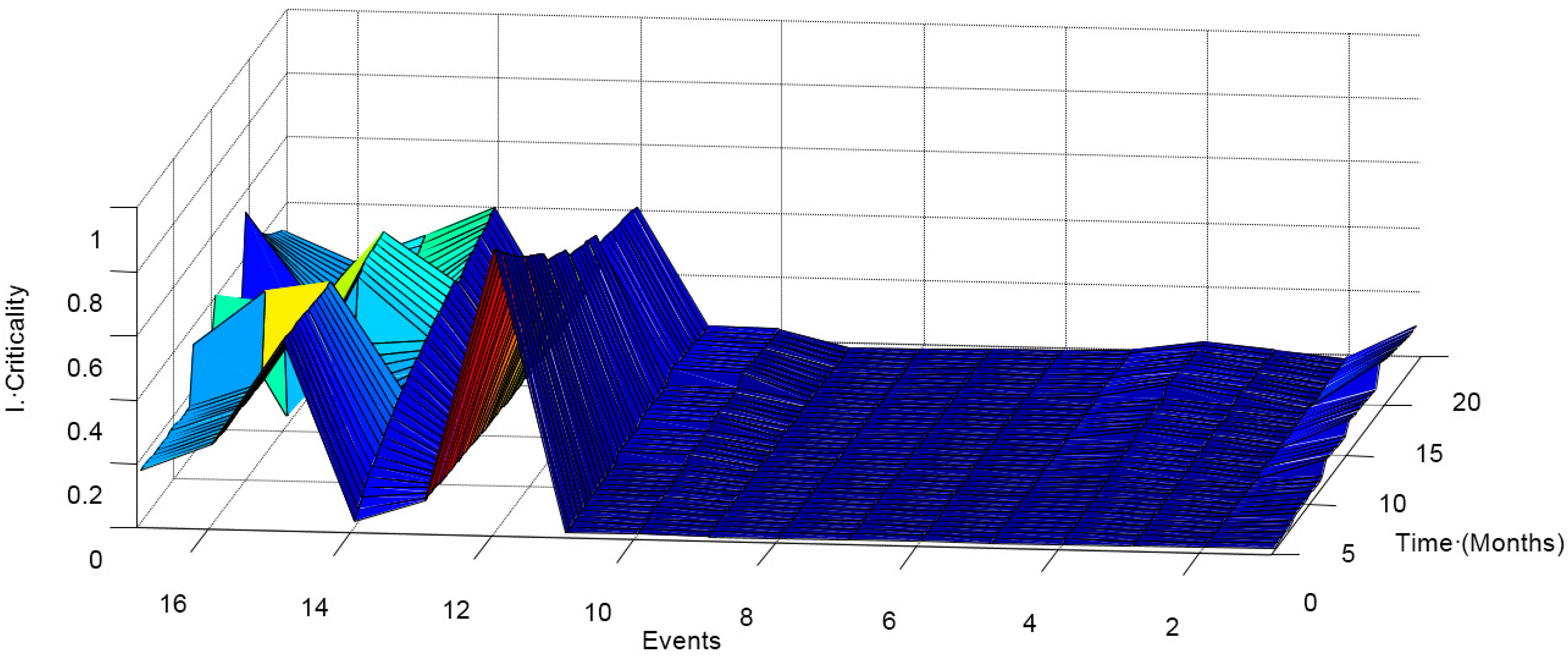
The Criticality method shows that the event e012 is the most important for the Qsys, followed by e0015 and e014 and, finally, by e016 and e017 (see Figure 13). The criticality enables the real risk of each failure to be evaluated considering not only the contribution of the event to the global system but also the probability of the event. From Figure 13 it can be gathered that, among the most critical failures, the short circuit is the most probable event. However, the open circuit does not represent an imminent risk in spite of being a very critical failure according to Birnbaum importance.
The Fussell-Vesely approach shows in Figure 14 that the principal event is e012, and then e014, e015, e016 and e017. Again, the most important event is the short circuit. The Fussel-vesely importance establishes the ratio in which the event belongs to the cause of the global failure. In this case, the presence of corrosion is very usual when a converter failure occurs.
The main conclusions are that the events from e001 to e011 have the lowest IMs, and the event e012 is the most important for Qsys, followed by the events e013, e014, e015, e016 and e017. Only the Birnbaum method demonstrates that the main events are e012, e013 and e014. Therefore, the event ‘short circuit’ should be studied in detail because all the methods provide a high IM value.
The dynamic analysis proposed in this paper can improve maintenance planning because the fault probability is known over time. The IMs allows classification of the main events or components that should be considered to reduce the system failure probability, and, therefore, to optimize the resources. This analysis can be employed for prognostics and diagnosis tasks.
5. Conclusions
The condition of the converters and the main electrical components in a WT has been analysed over time in this paper via fault tree analysis. In this work, binary decision diagrams are used to reduce the computational costs. The cut-sets (combination of basic events whose simultaneous occurrence causes the top event to happen) generated by binary decision diagrams, depending on the order of events. The “Level”, “Top-Down-Left-Right”, “AND”, “Depth-First Search” and “Breadth-First Search” methods have been considered for ranking the events, and a comparative analysis of them has been done. The methods AND, TDLR and Level have provided the minimum number of cut-sets, 99, whereas the DFS and BFS methods get 171 cut-sets.
An illustrative fault tree for converters and the main electrical components has been developed. The authors have followed the opinion of experts and research studies in establishing the set of events and their occurrence probabilities. Importance measures (Birnbaum, Criticality and Fussel-Vesely) have been used to identify the most critical events. A set of experiments were carried out where all the importance measures provided a similar solution: short circuit (electronics) is the most important event for the system reliability over time, followed by the open circuit (electronics), gate drive circuit, corrosion, dirty and terminals damage. Consequently, attention needs to be focused on these events to improve the reliability of the system.
The quantitative analysis proposed in this paper is robust and flexible. It allows system failure probability to be determined over time. The dynamic analysis proposed in this paper can be used to improve the maintenance planning. This novel approach can increase the accuracy of the system and allow a correct maintenance plan to be established.
Acknowledgments
The work reported herewith has been financially supported by the Spanish Ministerio de Economía y Competitividad, under Research Grants DPI2015-67264-P and RTC-2016-5694-3.
Author Contributions
All authors of this paper have participated in all the sections.
Conflicts of Interest
The authors declare no conflict of interest.
Abbreviations
| BDD | Binary decision diagram |
| BFS | Breadth-first search |
| CMS | Condition monitoring system |
| CS | Cut-set |
| DFIG | Doubly fed induction generator |
| DFS | Depth-first search |
| FT | Fault tree |
| GWEC | Global wind energy council |
| IGBT | Insulated gate bipolar transistor |
| IM | Importance measure |
| O&M | Operation and maintenance |
| PFE | power feed equipment |
| PMSG | permanent magnet synchronous generator |
| PWM | pulse width modulation |
| SCADA | Supervisory control and data acquisition system |
| TDLR | Top-Down-Left-Right |
| WT | Wind turbine |
| 3L-NPC-BTB | Three-Level Neutral-Point Diode Clamped Back-To-Back |
| 2L-BTB | Two-level back-to-back voltage source converter |
| Formula Expressions | |
| CS | Cut-set |
| Qsys | Unavailability of the system |
| Probability of the event ‘ i’ over time | |
| probability rising velocity | |
| period size | |
| Constant | |
References
- Global Wind Energy Council (GWEC). Global Wind Report: Annual Market Update 2016. Available online: www.gwec.net (accessed on June 2017).
- Pérez, J.M.P.; Márquez, F.P.G.; Hernández, D.R. Economic viability analysis for icing blades detection in wind turbines. J. Clean. Prod. 2016, 135, 1150–1160. [Google Scholar] [CrossRef]
- Walford, C. Wind Turbine Reliability: Understanding and Minimizing Wind Turbine Operation and Maintenance Costs; Sandia Report, SAND2006-1100; Sandia National Laboratories: Albuquerque, NM, USA; Livermore, CA, USA, 2006. [Google Scholar]
- Novaes, G.; Araújoa, A.M.; Carvallo, P.A. Prognostic techniques applied to maintenance of wind turbines: A concise and specific review. Renew. Sustain. Energy Rev. 2017, in press. [Google Scholar]
- Tavner, P.J.; van Bussel, G.J.W.; Koutoulakos, E. Reliability of Different Wind Turbine Concepts with Relevance to Offshore Application. In Proceedings of the European Wind Energy Conference, Brussels, Belgium, 31 March–3 April 2008. [Google Scholar]
- Anonymous. Managing the Wind: Reducing Kilowatt-Hour Costs with Condition Monitoring. Refocus 2005, 6, 48–51. [Google Scholar]
- Márquez, F.P.G.; Muñoz, J.M.C. A pattern recognition and data analysis method for maintenance management. Int. J. Syst. Sci. 2012, 43, 1014–1028. [Google Scholar] [CrossRef]
- Munoz, J.C.; Márquez, F.G.; Papaelias, M. Railroad inspection based on ACFM employing a non-uniform B-spline approach. Mech. Syst. Sign. Process. 2013, 40, 605–617. [Google Scholar] [CrossRef]
- Pliego, A.; Garcia, F.P.; Pinar, J.M. Optimal Maintenance Management of Offshore Wind Farms. Energies 2016, 9, 46. [Google Scholar] [CrossRef]
- De Novaes Pires, G.; Alencar, E.; Kraj, A. Remote Conditioning Monitoring System for a Hybrid Wind Diesel System-Application at Fernando de Naronha Island, Brasil. Available online: http://www.ontario-sea.org (accessed on 19 July 2010).
- Polinder, H.; Bang, D.J.; Li, H.; Chen, Z. Concept Report on Generator Topologies, Mechanical and Electromagnetic Optimization. Proj. UpWind 2007. [Google Scholar]
- Hansen, A.D.; Lov, F.; Blaabjerg, F.; Hansen, L.H. Review of contemporary wind turbine concepts and their market penetration. Wind Eng. 2004, 28, 247–263. [Google Scholar] [CrossRef]
- Hansen, A.D.; Hansen, L.H. Wind turbine concept market penetration over 10 years (1995–2004). Wind Energy 2007, 10, 81–97. [Google Scholar] [CrossRef]
- Li, H.; Chen, Z. Overview of different wind generator systems and their comparisons. Renew. Power Gener. IET 2008, 2, 123–138. [Google Scholar] [CrossRef]
- Argyriadis, K.; Rademakers, L.; Capellaro, K.; Ristow, M.; Hauptmann, S.; Kochmann, M.; Mouzakis, F. PROTEST (PROcedures for TESTing and measuring wind energy systems). In Deliverable D1: State-of-the-Art-Report; FP7-ENERGY-2007-1-RTD; University of Stuttgart: Stuttgart, Germany, 2009. [Google Scholar]
- Igarashi, T.; Hamada, H. Studies on the Vibration and Sound of Defective Roller Bearings (First report: Vibration of ball bearing with one defect). Bull. JSME 1982, 25, 994–1001. [Google Scholar] [CrossRef]
- Igarashi, T.; Yabe, S. Studies on the Vibration and Sound of Defective Roller Bearings (First report: Sound of ball bearing with one defect). Bull. JSME 1983, 26, 1791–1798. [Google Scholar] [CrossRef]
- Gómez, C.Q.; Ruiz, R.; Trapero, J.R.; Marquez, F.P.G. A novel approach to fault detection and diagnosis on wind turbines. Glob. NEST J. 2014, 16, 1029–1037. [Google Scholar]
- Nabati, E.G.; Thoben, K.D. Big Data Analytics in the Maintenance of Off-Shore Wind Turbines: A Study on Data Characteristics. In Dynamics in Logistics; Springer: Basel, Switzerland, 2017; pp. 131–140. [Google Scholar]
- Gómez, C.Q.; Marquez, F.P.G. A New Fault Location Approach for Acoustic Emission Techniques in Wind Turbines. Energies 2016, 9, 40. [Google Scholar] [CrossRef]
- Pedregal, D.J.; Garcia, F.P.; Roberts, C. An Algorithmic Approach for Maintenance Management. Ann. Oper. Res. 2009, 166, 109–124. [Google Scholar] [CrossRef]
- Marquez, F.P.G.; Pliego, A.; Lorente, J.; Trapero, J. A new ranking approach for Decision Making in Maintenance Management. In Proceedings of the Seventh International Conference on Management Science and Engineering Management, Philadelphia, PA, USA, 7–9 November 2013; Lecture Notes in Electrical Engineering. Springer: Berlin, Germany; pp. 27–38. [Google Scholar]
- Marquez, F.P.G.; Roberts, C.; Tobias, A. Railway Point Mechanisms: Condition Monitoring and Fault Detection. Proc. Inst. Mech. Eng. Part F 2010, 224, 35–44. [Google Scholar] [CrossRef]
- Marquez, F.P.G.; Pedregal, D.J.; Roberts, C. Time Series Methods Applied to Failure Prediction and Detection. Reliab. Eng. Syst. Saf. 2010, 95, 698–703. [Google Scholar]
- Ruiz, R.; Garcia, F.P.; Dimlaye, V. Maintenance management of wind turbines structures via MFCs and wavelet transforms. Renew. Sustain. Energy Rev. 2015, 48, 472–482. [Google Scholar]
- Levitin, G. Genetic Algorithms in Reliability Engineering. Reliab. Eng. Syst. Saf. 2006, 91, 975–976. [Google Scholar] [CrossRef]
- Development and Demonstration of a Novel Integrated Condition Monitoring System for Wind Turbines, NIMO Project. (NIMO, Ref.:FP7-ENERGY-2008-TREN-1: 239462). Available online: www.nimoproject.eu (accessed on 30 January 2012).
- Demonstration of Methods and Tools for the Optimisation of Operational Reliability of Large-Scale Industrial Wind Turbines, OPTIMUS Project. (OPTIMUS, Ref.: FP-7-Energy-2012-TREN-1: 322430). Available online: www.optimusproject.eu (accessed on 25 February 2014).
- McMillan, D.; Ault, G. Specification of reliability benchmarks for offshore wind farms. In Proceedings of the European Safety and Reliability, Valencia, Spain, 22–25 September 2008; CRC Press: Cleveland, OH, USA, 2008; pp. 22–25. [Google Scholar]
- Lu, B.; Li, Y.; Wu, X.; Yang, Z. A Review of Recent Advances in WT Condition Monitoring and Fault Diagnosis. In Proceedings of the Power Electronics and Machines in Wind Applications, Lincoln, NE, USA, 24–26 June 2009. [Google Scholar]
- Ciang, C.C.; Lee, J.R.; Bang, H.-J. Structural health monitoring for a WT system: A review of damage detection methods. Meas. Sci. Technol. 2008, 19, 22. [Google Scholar] [CrossRef]
- Hansena, D.; Michalke, G. Fault ride-through capability of DFIG wind turbines. Renew. Energy 2007, 32, 1594–1610. [Google Scholar] [CrossRef]
- Douglas, H.; Pillay, P.; Ziarani, A. Broken rotor bar detection in induction machines with transient operating speeds. IEEE Trans. Energy Convers. 2005, 20, 135–141. [Google Scholar] [CrossRef]
- Fischer, K.; Besnard, F.; Bertling, L. A Limited-Scope Reliability-Centred Maintenance Analysis of Wind Turbines. In Proceedings of the European Wind Energy Conference EWEA, Brussels, Belgium, 14–17 March 2011; pp. 89–93. [Google Scholar]
- Popa, L.M.; Jensen, B.B.; Ritchie, E.; Boldea, I. Condition monitoring of wind generators. In Proceedings of the Industry Applications Conference, 38th IAS Annual Meeting, Salt Lake City, UT, USA, 12–16 October 2003; pp. 1839–1846. [Google Scholar]
- Liu, W.; Tang, B.; Jiang, Y. Status and problems of WT structural health monitoring techniques in China. Renew. Energy 2010, 35, 1414–1418. [Google Scholar] [CrossRef]
- Wang, H.; Ma, K.; Blaabjerg, F. Design for reliability of power electronic systems. In Proceedings of the IECON 2012—38th Annual Conference on IEEE Industrial Electronics Society, Montreal, QC, Canada, 25–28 October 2012; pp. 33–44. [Google Scholar]
- RELIAWIND Project. European Union’s Seventh Framework Programme for RTD (FP7). Available online: http://www.reliawind.eu/ (accessed on January 2014).
- Arabian-Hoseynabadi, H.; Oraee, H.; Tavner, P.J. Failure Modes and Effects Analysis (FMEA) for Wind Turbines. Int. J. Electr. Power Energy Syst. 2010, 32, 817–824. [Google Scholar] [CrossRef] [Green Version]
- International Electrotechnical Commission. 2005–2008 Wind Turbines—Part 1: Design Requirements, 3rd ed.; IEC 61400-1; International Electrotechnical Commission: Geneva, Switzerland, 2005. [Google Scholar]
- Schoen, R.R.; Lin, B.K.; Habetler, T.G.; Schlag, J.H.; Farag, S. An Unsupervised, On-Line System for Induction Motor Fault Detection Using Stator Current Monitoring. IEEE Trans. Ind. Appl. 1995, 31, 1280–1286. [Google Scholar] [CrossRef]
- Entezami, M.; Hillmansen, S.; Weston, P.; Papaelias, M. Fault detection and diagnosis within a wind turbine mechanical braking system using condition monitoring. Renew. Energy 2012, 47, 175–182. [Google Scholar] [CrossRef]
- Seo, D.C.; Lee, J.J. Damage detection of CFRP laminates using electrical resistance measurement and neural network. Compos. Struct. 1999, 47, 525–530. [Google Scholar] [CrossRef]
- Smith, B.M. Condition Monitoring by Thermography. NDT Int. 1978, 11, 121–122. [Google Scholar] [CrossRef]
- Gómez, C.Q.; Garcia, F.P.; Sanchez, J.M. Ice detection using thermal infrared radiometry on wind turbine blades. Measurement 2016, 93, 157–163. [Google Scholar] [CrossRef]
- Rumsey, M.A.; Musial, W. Application of Infrared Thermography Nondestructive Testing during Wind Turbine Blade Tests. J. Sol. Energy Eng. 2001, 123, 271. [Google Scholar] [CrossRef]
- Doliński, L.; Krawczuk, M. Damage detection in turbine wind blades by vibration based methods. In Proceedings of the 7th International Conference on Modern Practice in Stress and Vibration Analysis, Cambridge, UK, 8–10 September 2009. [Google Scholar]
- Blaabjerg, F.; Liserre, M.; Ma, K. Power electronics converters for wind turbine systems. IEEE Trans. Ind. Appl. 2012, 48, 708–719. [Google Scholar] [CrossRef]
- Alrifai, M.; Zribi, M.; Rayan, M. Feedback Linearization Controller for a Wind Energy Power System. Energies 2016, 9, 771. [Google Scholar] [CrossRef]
- Xu, P.; Shi, K.; Bu, F.; Zhao, D.; Fang, Z.; Liu, R.; Zhu, Y. A Vertical-Axis Off-Grid Squirrel-Cage Induction Generator Wind Power System. Energies 2016, 9, 822. [Google Scholar] [CrossRef]
- Xiao, Y.; Zhang, T.; Ding, Z.; Li, C. The study of fuzzy proportional integral controllers based on improved particle swarm optimization for permanent magnet direct drive wind turbine converters. Energies 2016, 9, 343. [Google Scholar] [CrossRef]
- Masahiro, F.; Hisanori, F.; Bobuaki, K. Evaluation and Improvements of Boolean Comparison. In Method Based on Binary Decision Diagrams; Fujitsu Laboratories LTD: Hayes, UK, 1988. [Google Scholar]
- Lee, C.Y. Representation of switching circuits by binary-decision programs. Bell Syst. Tech. J. 1959, 38, 985–999. [Google Scholar] [CrossRef]
- Moret, B.M.E. Decision trees and diagrams. ACM Comput. Surv. 1982, 14, 413–416. [Google Scholar] [CrossRef]
- Pliego, A.; García, F.P.; Lev, B. Optimal decision-making via binary decision diagrams for investments under a risky environment. Int. J. Prod. Res. 2017, 55, 1–16. [Google Scholar]
- Stol, K.A. Disturbance tracking control and blade load mitigation for variable speed wind turbines. J. Sol. Energy Eng. 2003, 125, 396–401. [Google Scholar] [CrossRef]
- Bartlett, L.M. Progression of the Binary Decision Diagram Conversion Methods. In Proceedings of the 21st International System Safety Conference, Ottawa, ON, Canada, 4–8 August 2003; pp. 116–125. [Google Scholar]
- Cormen, T.H.; Leiserson, C.E.; Rivest, R.L.; Stein, C. Introduction to Algorithms, 2nd ed.; Section 22.3: Depth-First Search; MIT Press: Cambridge, MA, USA; McGraw-Hill: New York, NY, USA, 2001; pp. 540–549. ISBN 0-262-03293-7. [Google Scholar]
- Jensen, R.; Veloso, M. OBDD-Based Universal Planning for Synchronized Agents in Non-Deterministic Domains. J. Artif. Intell. Res. 2000, 13, 189–226. [Google Scholar]
- Malik, S.; Wang, A.R.; Brayton, R.K.; Vincentelli, A.S. Logic Verification using Binary Decision Diagrams in Logic Synthesis Environment. In Proceedings of the IEEE International Conference on Computer Aided Design, ICCAD’88, Santa Clara, CA, USA, 7–10 November 1988; pp. 6–9. [Google Scholar]
- Xie, M.; Tan, K.C.; Goh, K.H.; Huang, X.R. Optimum Prioritisation and Resource Allocation Based on Fault Tree Analysis. Int. J. Qual. Reliab. Manag. 2000, 17, 189–199. [Google Scholar] [CrossRef]
- Birnbaum, Z.W. On the Importance of Different Components in a Multicomponent System; Academic Press: New York, NY, USA, 1969; pp. 581–592. [Google Scholar]
- Lambert, H.E. Measures of importance of events and cut sets. In Reliability and Fault Tree Analysis; SIAM: Philadelphia, PA, USA, 1975; pp. 77–100. [Google Scholar]
- Mankamo, T.; Pörn, K.; Holmberg, J. Uses of Risk Importance Measures; Technical Report, Research Notes 1245; Technical Research Centre of Finland: Espoo, Finland, 1991; ISBN 951-38-3877-3. ISSN 0358-5085. [Google Scholar]
- Swain, S.; Ray, P.K. Short circuit fault analysis in a grid connected DFIG based wind energy system with active crowbar protection circuit for ridethrough capability and power quality improvement. Int. J. Electr. Power Energy Syst. 2017, 84, 64–75. [Google Scholar] [CrossRef]
- Qiu, Y.; Jiang, H.; Feng, Y.; Cao, M.; Zhao, Y.; Li, D. A new fault diagnosis algorithm for PMSG wind turbine power converters under variable wind speed conditions. Energies 2016, 9, 548. [Google Scholar] [CrossRef]
- De Moura, E.P.; de Abreu Melo Junior, F.E.; Damasceno, F.F.R.; Figueiredo, L.C.C.; de Andrade, C.F.; de Almeida, M.S.; Rocha, P.A.C. Classification of imbalance levels in a scaled wind turbine through detrended fluctuation analysis of vibration signals. Renew. Energy 2016, 96, 993–1002. [Google Scholar]
- Faiz, J.; Moosavi, S.M.M. Eccentricity fault detection—From induction machines to DFIG—A review. Renew. Sustain. Energy Rev. 2016, 55, 169–179. [Google Scholar]
- Hameed, Z.; Hong, Y.S.; Cho, Y.M.; Ahn, S.H.; Song, C.K. Condition monitoring and fault detection of WTs and related algorithms: A review. Renew. Sustain. Energy Rev. 2009, 13, 1–39. [Google Scholar] [CrossRef]
- Wu, A.P.; Chapman, P.L. Simple expressions for optimal current waveforms for permanent-magnet synchronous machine drives. IEEE Trans. Energy Convers. 2005, 20, 151–157. [Google Scholar] [CrossRef]
- Garcia, F.P.; Pinar, J.M.; Pliego, A.; Papaelias, M. Identification of critical components of wind turbines using FTA over time. Renew. Energy 2016, 85, 1178–1191. [Google Scholar]
- Pliego, A.; Garcia, F.P. A Novel Approach on Diagnostic and Prognostics in Railways: A Real Case Study. Proc. Inst. Mech. Eng. Part F J. Rail Rapid Transit 2015, 230, 1440–1456. [Google Scholar] [CrossRef]
Figure 1.
Distribution of failure frequencies between different turbine types, sorted by turbine size (Adapted from [5]).
Figure 1.
Distribution of failure frequencies between different turbine types, sorted by turbine size (Adapted from [5]).
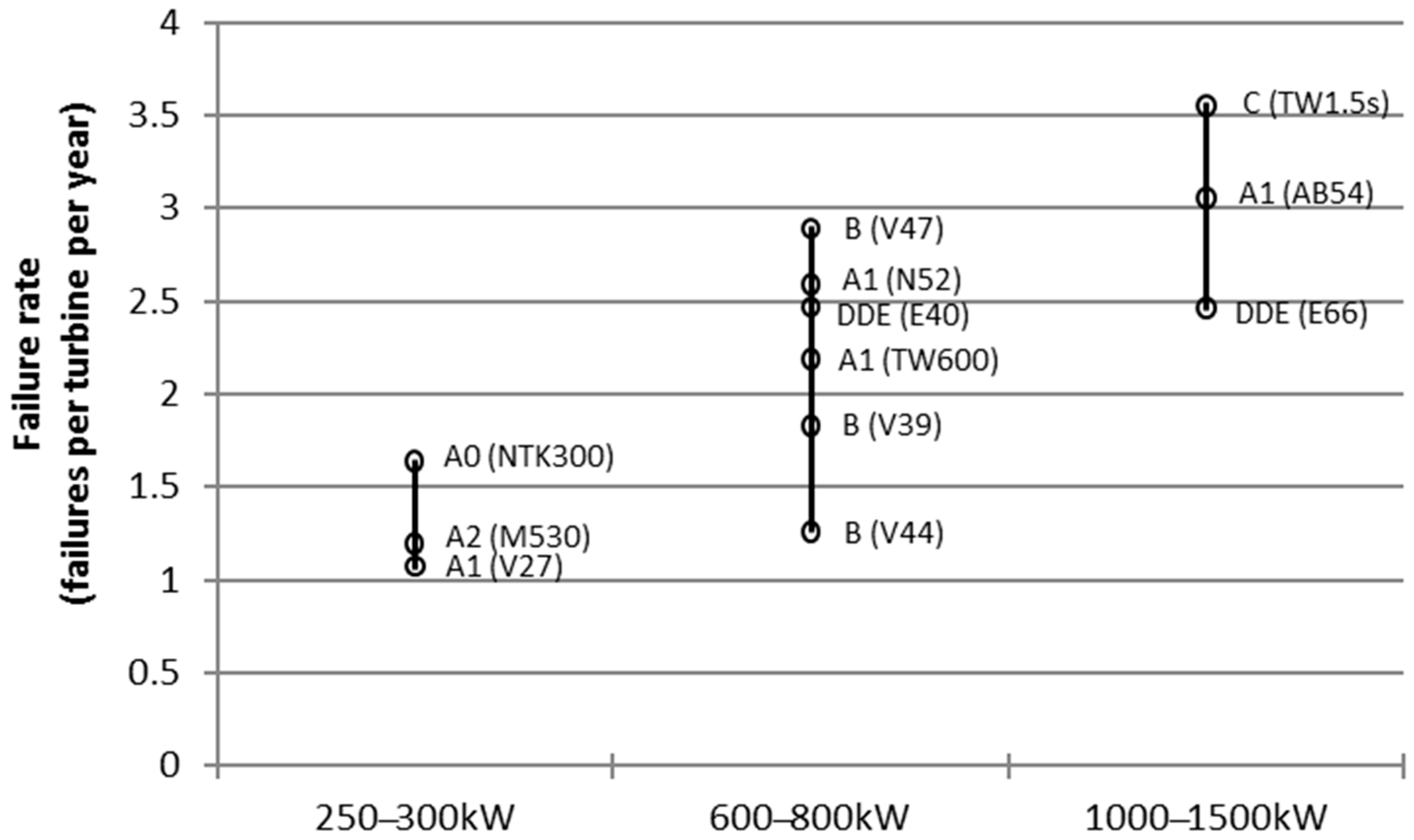
Figure 2.
Main components of the most installed WT where: 1—pitch system; 2—hub; 3—main bearing; 4—low speed shaft; 5—gearbox; 6—high speed shaft; 7—brake system; 8—generator; 9—yaw system; 10—bedplate; 11—converter; 12—tower; 13—meteorological unit. (Adapted from [10]).
Figure 2.
Main components of the most installed WT where: 1—pitch system; 2—hub; 3—main bearing; 4—low speed shaft; 5—gearbox; 6—high speed shaft; 7—brake system; 8—generator; 9—yaw system; 10—bedplate; 11—converter; 12—tower; 13—meteorological unit. (Adapted from [10]).
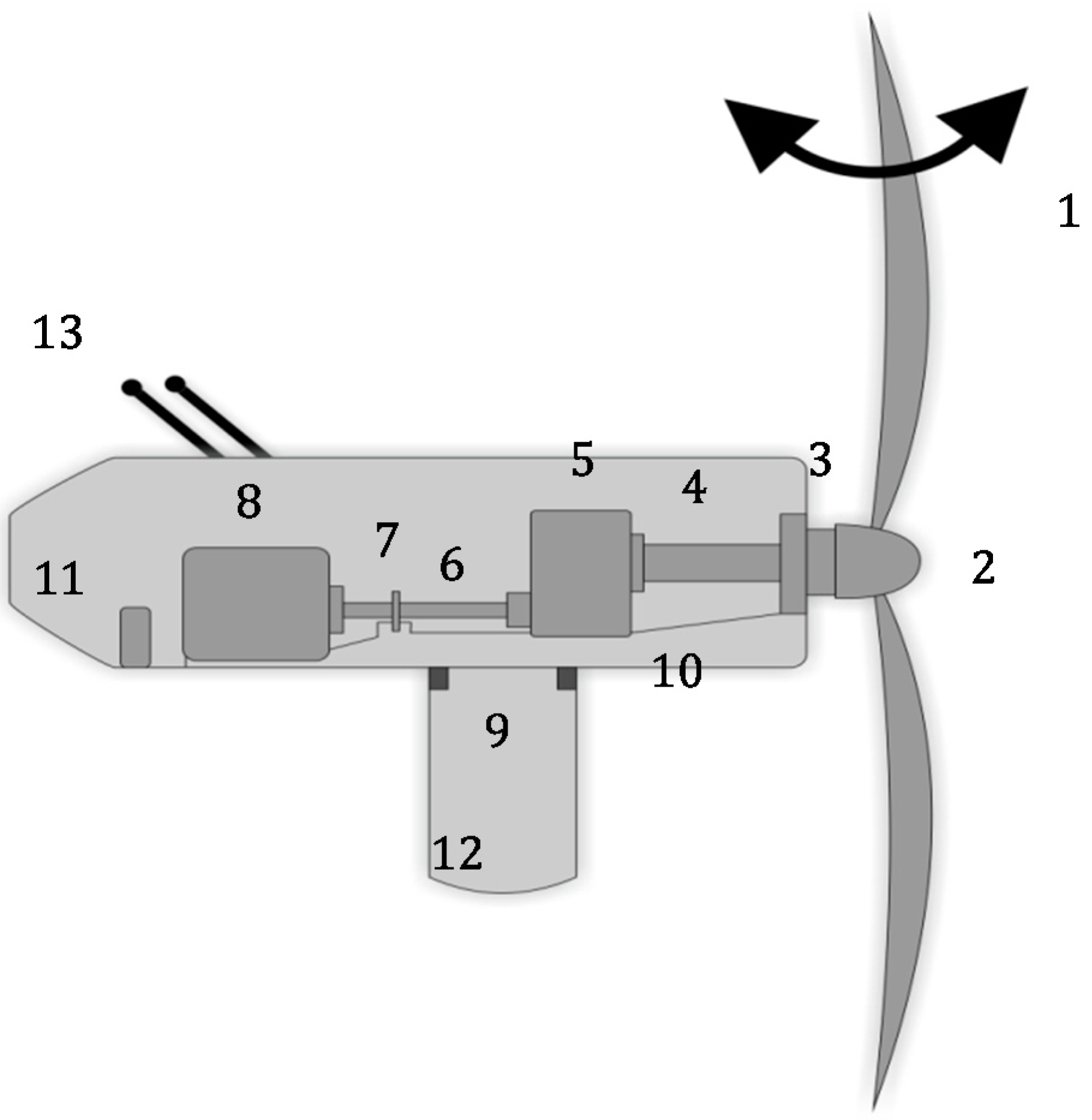
Figure 3.
Distribution of the component costs for a typical 2 MW wind turbines (adapted from [15]).
Figure 3.
Distribution of the component costs for a typical 2 MW wind turbines (adapted from [15]).
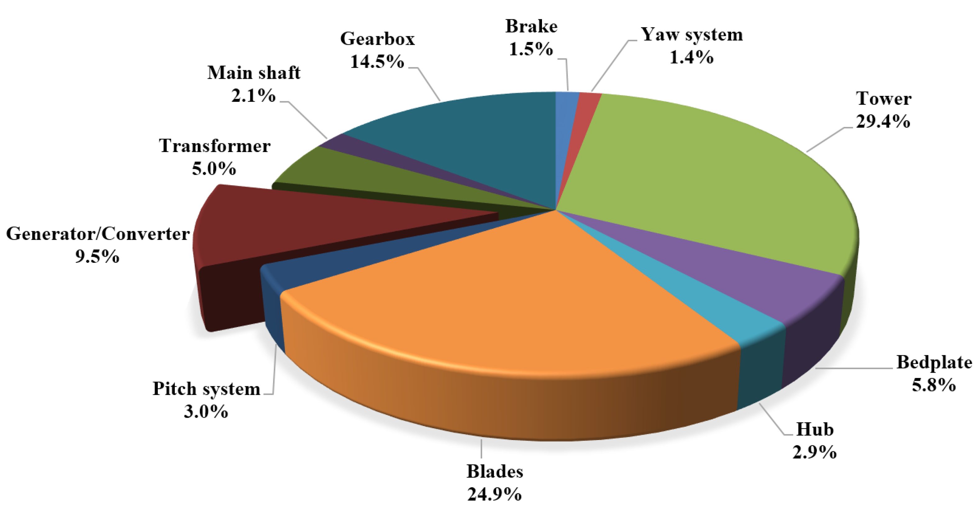
Figure 4.
Annual failure probability for subcomponents (adapted from [29]).
Figure 4.
Annual failure probability for subcomponents (adapted from [29]).

Figure 5.
Failure root cause distribution (adapted from [37]).
Figure 5.
Failure root cause distribution (adapted from [37]).
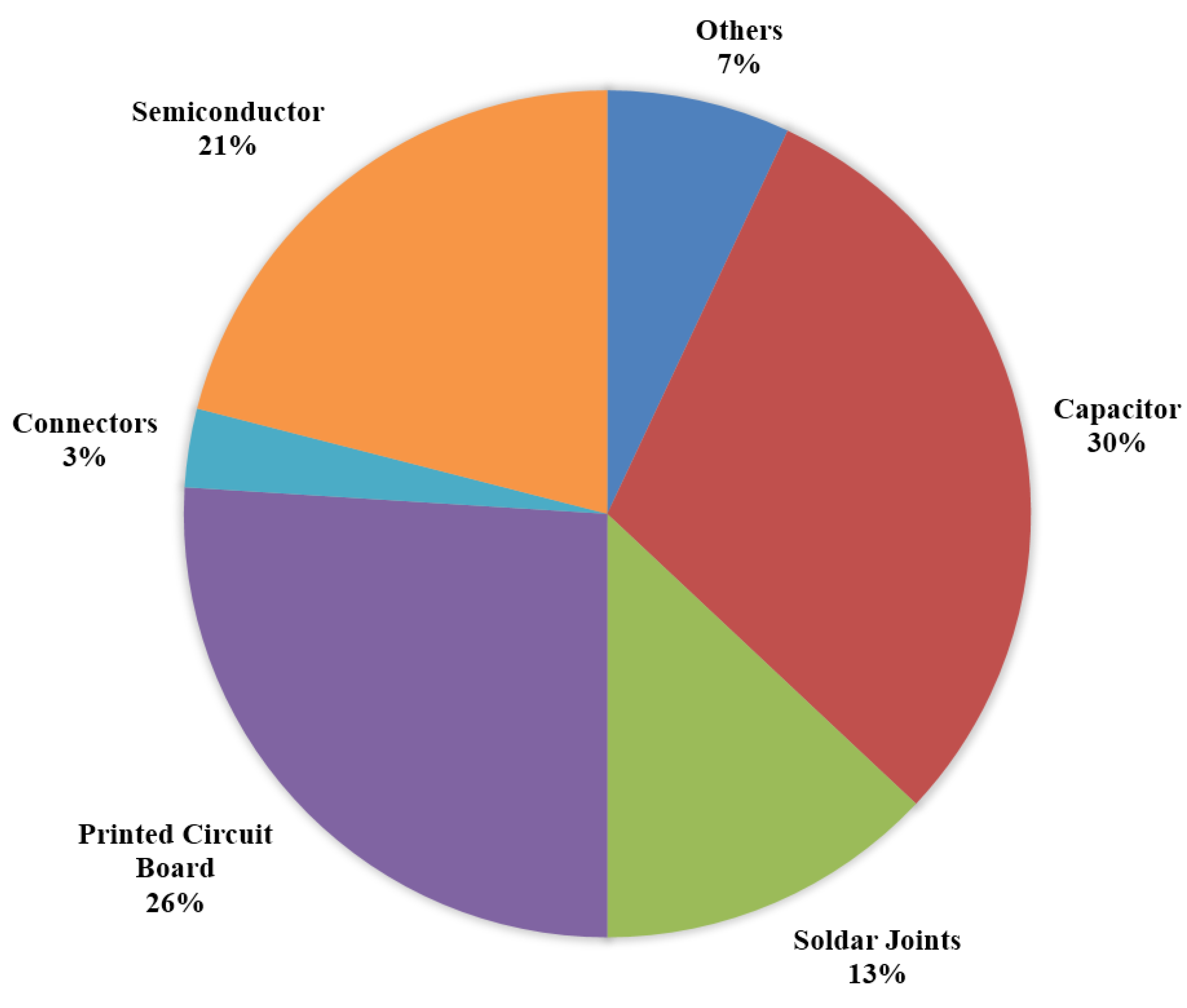
Figure 6.
The current sensors for the brake hydraulic system inside the main control panel of the WT Reproduced with permission from [42]. Elsevier, 2012.
Figure 6.
The current sensors for the brake hydraulic system inside the main control panel of the WT Reproduced with permission from [42]. Elsevier, 2012.

Figure 7.
Fault Tree example.

Figure 8.
Fault tree of the generator, electrical and electronic components.

Figure 9.
Probability over time for each event of Figure.

Figure 10.
Qsys(t) over time.
Figure 11.
Qsys(t) with time variable increment.

Figure 12.
Birnbaum importance for each event over time.
Figure 13.
Critically importance for each event over time.

Figure 14.
Fussel-Vesely importance for each event over time.

Table 1.
Number of Cut-Sets (CS).
| Ranking Method | TLDR | DFS | BFS | Level | AND |
|---|---|---|---|---|---|
| Number of CS | 46 | 31 | 36 | 46 | 35 |
Table 2.
Principal faults in the converter, generator, electrical and electronic components.
| Non-Basic Events | Basic Events | ||
|---|---|---|---|
| Critical Generator Failure | g001 | Abnormal Vibration G | e001 |
| Power electronics and electric controls failure | g002 | Cracks | e002 |
| Mechanical failure (generator) | g003 | Imbalance | e003 |
| Electrical failure (generator) | g004 | Asymmetry | e004 |
| Bearing generator failure | g005 | Air-Gap eccentricities | e005 |
| Rotor and stator failure | g006 | Broken bars | e006 |
| Bearing generator fault | g007 | Dynamic eccentricity | e007 |
| Rotor and stator fault | g008 | Sensor Tª error | e008 |
| Abnormal signals A | g009 | Temperature above limit | e009 |
| Overheating generator | g010 | Short circuit (generator) | e010 |
| Electrical fault (PE) | g011 | Open circuit (generator) | e011 |
| Mechanical fault (PE) | g012 | Short circuit (electronics) | e012 |
| Open circuit (electronics) | e013 | ||
| Gate drive circuit | e014 | ||
| Corrosion | e015 | ||
| Dirt | e016 | ||
| Terminals damage | e017 | ||
Table 3.
Ranking methods and CSs.
| Ranking Method | Number of CSs |
|---|---|
| TDLR | 99 |
| DFS | 171 |
| BFS | 171 |
| Level | 99 |
| AND | 99 |
| Event | Probability Model | Parameters |
|---|---|---|
| e001 | Exponential increasing | 𝜆 = 0.0030 months−1 |
| e002 | Constant | K = 0.0010 |
| e003 | Exponential increasing | 𝜆 = 0.0025 months−1 |
| e004 | Exponential increasing | 𝜆 = 0.0045 months−1 |
| e005 | Linear increasing | m = 0.0015 months−1 |
| e006 | Linear increasing | m = 0.0009 months−1 |
| e007 | Linear increasing | m = 0.0007 months−1 |
| e008 | Constant | K = 0.0040 |
| e009 | Periodic | 𝜆 = 0.0025 months−1, = 5 months |
| e010 | Constant | K = 0.0012 |
| e011 | Constant | K = 0.0013 |
| e012 | Constant | K = 0.0020 |
| e013 | Constant | K = 0.0021 |
| e014 | Linear increasing | m = 0.0010 months−1 |
| e015 | Periodic | 𝜆 = 0.0035 months−1, = 7 months |
| e016 | Periodic | 𝜆 = 0.0015 months−1, = 10 months |
| e017 | Linear increasing | m = 0.0010 months−1 |
© 2017 by the authors. Licensee MDPI, Basel, Switzerland. This article is an open access article distributed under the terms and conditions of the Creative Commons Attribution (CC BY) license (http://creativecommons.org/licenses/by/4.0/).
Share and Cite
MDPI and ACS Style
García Márquez, F.P.; Pliego Marugán, A.; Pinar Pérez, J.M.; Hillmansen, S.; Papaelias, M. Optimal Dynamic Analysis of Electrical/Electronic Components in Wind Turbines. Energies 2017, 10, 1111. https://doi.org/10.3390/en10081111
AMA Style
García Márquez FP, Pliego Marugán A, Pinar Pérez JM, Hillmansen S, Papaelias M. Optimal Dynamic Analysis of Electrical/Electronic Components in Wind Turbines. Energies. 2017; 10(8):1111. https://doi.org/10.3390/en10081111
Chicago/Turabian StyleGarcía Márquez, Fausto Pedro, Alberto Pliego Marugán, Jesús María Pinar Pérez, Stuart Hillmansen, and Mayorkinos Papaelias. 2017. "Optimal Dynamic Analysis of Electrical/Electronic Components in Wind Turbines" Energies 10, no. 8: 1111. https://doi.org/10.3390/en10081111
Note that from the first issue of 2016, this journal uses article numbers instead of page numbers. See further details here.