Development of the IBSAL-SimMOpt Method for the Optimization of Quality in a Corn Stover Supply Chain


1
Mechanical Engineering Department, The University of Texas at San Antonio, One UTSA Circle, San Antonio, TX 78249, USA
2
Environmental Sciences Division, Oak Ridge National Laboratory, One Bethel Rd., Oak Ridge, TN 37831, USA
*
Author to whom correspondence should be addressed.
Energies 2017, 10(8), 1137; https://doi.org/10.3390/en10081137
Submission received: 28 June 2017
/
Revised: 31 July 2017
/
Accepted: 31 July 2017
/
Published: 3 August 2017
(This article belongs to the Special Issue Biomass for Energy Country Specific Show Case Studies)
Abstract
:Variability on the physical characteristics of feedstock has a relevant effect on the reactor’s reliability and operating cost. Most of the models developed to optimize biomass supply chains have failed to quantify the effect of biomass quality and preprocessing operations required to meet biomass specifications on overall cost and performance. The Integrated Biomass Supply Analysis and Logistics (IBSAL) model estimates the harvesting, collection, transportation, and storage cost while considering the stochastic behavior of the field-to-biorefinery supply chain. This paper proposes an IBSAL-SimMOpt (Simulation-based Multi-Objective Optimization) method for optimizing the biomass quality and costs associated with the efforts needed to meet conversion technology specifications. The method is developed in two phases. For the first phase, a SimMOpt tool that interacts with the extended IBSAL is developed. For the second phase, the baseline IBSAL model is extended so that the cost for meeting and/or penalization for failing in meeting specifications are considered. The IBSAL-SimMOpt method is designed to optimize quality characteristics of biomass, cost related to activities intended to improve the quality of feedstock, and the penalization cost. A case study based on 1916 farms in Ontario, Canada is considered for testing the proposed method. Analysis of the results demonstrates that this method is able to find a high-quality set of non-dominated solutions.
1. Introduction
Biofuel has been recognized as an alternative source of renewable energy [1]. This research focuses on the use of energy crops, agricultural and forest residues to produce second-generation biofuels. First-generation biofuels are produced using edible products such as corn and soybean. These types of biomass feedstock have raised the debate of food versus fuel and, as a result, second-generation biofuels were developed. Second generation biomass feedstock exhibit more variability on its physical properties (e.g., higher ash and moisture contents) than first generation biomass. The variability of these physical properties has an important effect on the cost to deliver biomass feedstock to the reactor throat, which is known as delivered cost [2]. This delivered cost includes the cost of production, harvest, storage, handling, preprocessing, and transportation operations. Particularly, the cost of production includes the cost of feedstock, which accounts for 40–60% of the operating cost of conversion facilities [3,4].
The term “biorefinery” refers to the facility that processes biomass coming from plant, animal and food wastes into energy, fuels, chemicals, polymers, and food additives, among others [5]. At a constant operation rate, biorefinery processing facilities have lifetimes of 20 to 25 years [6]. Considering such a limited time for biorefineries to obtain profit on their investment, it becomes extremely important that all factors that have a direct effect on the delivered cost are considered when developing a bioenergy project. However, it is not possible to maintain delivered cost at a level that supports the profitability of the bioenergy projects and allows reduction of fuel cost when it is not possible to maintain the required supply of convertible biomass (i.e., biomass with uniform physical characteristics at the specification values determined by the conversion process).
The purpose of this paper is to propose and test a Discrete Events Simulation (DES) model coupled with a metaheuristic-based optimization method to design and manage a biomass supply chain (SC). The SC spans from the collection of biomass to the delivery at the gate of the biorefinery for its conversion to biofuel. The objective is to minimize the cost of having imperfect biomass quality and total dry matter loss.
The proposed model is based on an extension of the IBSAL (Integrated Biomass Supply Analysis and Logistics) model developed by Sokhansanj et al. [7]. This time-dependent DES model with activity-based costing has been extensively used by Oak Ridge National Laboratory (ORNL) to estimate the collection, storage, and transportation costs in biomass logistic systems. These estimates have been considered by the U.S. Department of Energy (DoE) and the bioenergy industry for making decisions related to the supply of biomass for the production of biofuel. In this paper, the IBSAL model is extended. The extended version estimates the cost of imperfect quality of feedstock and evaluates its effect on the performance measures of the SC. The inherent variability in biomass quality is added as well as several preventive pre-processing operations. Moreover, the extended IBSAL is coupled with a novel SimMOpt (Simulation-based Multi-Objective Optimization) method that allows finding near-optimal solutions. This method uses a Simulated Annealing (SA) approach for multi-objective problems with stochastic elements included in its formulations. In this way, the IBSAL (previously used as a manual what-if scenario tool) is enhanced to find near-optimal designs while considering multiple competing objectives.
This paper is structured as follows: Section 2 presents a literature review on models for biomass SCs. Section 3 describes the methodology: (a) the impact of feedstock quality; (b) interaction between the extended IBSAL and the SimMOpt optimization method; (c) detailed description of the SimMOpt optimization method; and (d) extended IBSAL with quality related blocks. Section 4 describes the case study and provides the geographical and operational characteristics of the implementation. The SA schedules (algorithmic parameters) considered during the experimentation are also discussed in this section. Section 5 presents the results of the case study using different SA schedules. Results are evaluated by computing a hyper volume indicator to determine the ability of the model of producing Pareto-optimal fronts. Section 6 discuss the quality of the set of non-dominated solutions for three SA schedules and future algorithmic improvements, which are intended to reduce the computational cost.
2. Literature Review
The delivered cost is highly sensitive to the variability on the attributes behavior (i.e., the properties of the elements intervening in the SC), and the interactions among them. Therefore, it is important to build models that realistically represent this variability and complex interactions, so that any conclusion based on the results from the experimentations with these models can be validated before design and management decisions are made to the real system. Reliable models, correct assumptions and accurate cost estimates are vital to appropriately design the system that will supply the feedstock to the conversion process.
Success in designing a biomass SC that optimizes the delivered cost depends on the model’s ability to: (1) represent the behavior of the elements intervening in the SC; (2) consider plausible assumptions; and (3) perform the computations within a reasonable computational burden.
These models are commonly based on approaches such as simulation-based optimization or mathematical programming (MP). Simulation-based optimization models may require a considerable amount of execution time and data. Alternatively, in some cases, it is possible to formulate simpler time-independent models using methods such as metaheuristics or MP. Consequentially, there is a price to pay for using simplified models to represent complex systems.
Two factors that contribute to the complexity of the models are: (1) stochastic behavior; and (2) competition among the performance indicators (e.g., multiple criteria/objectives). Solving multi-objective stochastic programming models may require complex solution techniques and considerable execution time. This becomes even more complex when the formulations include non-linear expressions, for instance, quadratic programming (QP). Instances that remain treatable within sensible execution time may be limited to those of highly constrained size. Ignoring stochastic behavior and merging competing objectives into a single function are usual practices for simplifying these models in many applications. These simplifications occur at the expense of detail in the model which may jeopardize its value as a representation of the SC.
One approach to dealing with multiple objectives consists of simplifying the problem by merging all objectives of interest into a single objective (i.e., a single mathematical expression). However, in many real cases in the bioenergy sector, the decision maker(s) (whether it is a farmer or a biorefinery) is interested in individual production, harvest, storage, handling, and transportation costs or some other performance measures such as dry matter loss, percentage of moisture, percentage of ash, probability of failing to meet the specifications at the conversion facility, instead of the single estimation of the overall costs (i.e., delivered cost). In supply chains, it is not unusual to find that the optimization of some performance measures frequently competes with the optimization of others [8]. Merging multiple objectives into a single performance measure prevents the decision maker(s) from conducting individual evaluations on each objective. An even more important, information on the behavior of each measure and interactions among them is lost when competing objectives are merged. In any case, a set of solutions for different scenarios and priorities provide the decision maker(s) with a better understanding on the behavior and interactions among individual objectives. This has motivated the development of models that can be used for the optimization of multiple competing performance measures in biomass SCs.
The applicability of these models, whether simplified or complex, to specific situations depend on the information required by the decision maker(s), the required level of detail in the modeling of the SC, the required level of resolution on the solutions, available input data, and available time for the execution of the model.
Many models in the literature are readily applicable to the minimization of the collection, storage, and transportation costs derived from supplying biomass to biorefineries for the production of biofuels. However, an appropriate design and integral evaluation of a SC must also consider the cost from having imperfect quality of feedstock. Table 1 mentions some papers that discuss the development and applications of models developed for the design and improvement of biomass SCs. The last column is reserved for indicating papers that are relevant to the development and implementation of the IBSAL model.
Some of the papers included Table 1 discuss the implementation of simulation-based methods for problems that consider multiple performance measures. The IBSAL model is used in some of these papers for: (1) searching for acceptable solutions; or (2) finding the value of some variables that serve as input parameters to other models proposed in that paper. Kumar et al. [9], and Kumar and Sokhansanj [10] present methodologies that use the IBSAL model for assessing alternatives for biomass collection and transportation systems while considering multiple performance measures (e.g., cost of delivered biomass, quality of biomass supplied, emissions during collection, energy input to the chain operation, and maturity of supply system technologies). Sokhansanj et al. [13] use the IBSAL model to estimate the economics (e.g., cost of collection, cost of pre-processing, transportation cost, on-site fuel storage and preparation costs, and overall delivered cost) of the supply of corn stover to produce heat and power for a drill mill ethanol plant. An and Searcy [16] use the IBSAL model to evaluate multiple performance measures (e.g., collection and processing cost, transportation cost, energy consumption, and CO2 emissions) in a biomass logistic system. Searcy and Hartley [20] utilize the IBSAL for evaluating a system of transportation and storage of herbaceous biomass in terms of volumetric percentages of different biomass quality classes.
Other works do not necessarily use the IBSAL model, but present an implementation of Discrete Event Simulation (DES) models for designing biomass SCs. Ravula et al. [11] use a DES model to determine the operation parameters of a cotton gin SC while considering multiple performance measures. They describe in detail some key components that cotton gin transportation systems share with biomass transportation systems. Igathinathane et al. [19] propose a simulation model to determine the bale storage configuration that minimizes the required time, fuel, and incurred cost from handling bales at the storage facility or field-stack. Pinho et al. [23] use SIMEVENTS®™ to build a DES model for a typical biomass production chain. The performance measures that are considered in this model include transportation time, chipping time, and idle time among others.
Some other papers in Table 1 propose simulation-based methods but focus more emphatically on a single performance measure (e.g., overall delivered cost). For instance, Stephen et al. [12] use the IBSAL model to assess the impact of agricultural residue yield on the delivered cost. Variability on physical properties of feedstock has a considerable effect on yield.
A second group includes papers that propose models based on non-simulation-based approaches, such as MP. An et al. [14] propose a MP model to maximize the profit of a lignocellulosic biofuel supply chain. The scope of the formulation covers from the feedstock suppliers to the biofuel customers. Shastri et al. [15] formulate a MILP model (e.g., BioFeed) to maximize the profit of the system (i.e., Miscanthus production and provision system). Other papers such as Larasati et al. [17] explain the dynamics between competing performance measures, such as the trade-off between switchgrass transportation cost and the economic scale of cellulosic ethanol production. Castillo-Villar et al. [24] use a QP model that merges the total cost of transportation, total cost of the harvest processes, cost for opening a collection of facilities, cost for opening a collection of biorefineries, mechanical drying cost, ash disposal cost, screening cost, grinding cost, and a penalty cost for reduced oil yield due to high ash content into a single cost function to be minimized.
Finally, a third group consists of those papers that propose integration between simulation and optimization. Ebadian et al. [18] integrate an optimization model and a simulation model for designing and planning of a bioethanol plant in Canada. They describe the limitations of the integral model and the effect of the termination criterion on its ability to meet a global optimal solution. Ren et al. [21] use a systems dynamics (SD) approach to analyze the corn stover and sweet sorghum supply systems and estimate the logistic costs. Chavez et al. [22] propose a simulation-based optimization model for minimizing two competing objectives in a supply chain of perishable commodities.
The papers mentioned in section “Development of the IBSAL Model” in Table 1 describe in detail the IBSAL model, new versions of the IBSAL (e.g., Ebadian et al. [26]), or a methodology that the authors of this paper found relevant in successfully integrating an optimization methodology with the IBSAL model.
Section “Availability of Feedstock and Technologies” in Table 1 includes papers that provide insight into the effect of weather and time on the physical properties of feedstock as it moves along the supply chain. It also includes a paper that provides solid ground for the selection of the case study. Kadam and McMillan [29] state that about 60–80 million dry tonne/yr of stover can be potentially available for ethanol production. The importance of corn stover as a source of biomass (particularly in some regions) supports the selection of the case study presented in this paper.
3. Methodology
3.1. The Impact of Feedstock Quality
In this study, two physical characteristics of the feedstock are used to quantify the quality of feedstock: (1) percentage of moisture content; and (2) percentage of ash. The SimMOpt model presented in this paper considers six goals during the optimization: (a) minimization of dry matter loss; (b) minimization of cost related to the implementation of activities intended to improve the physical characteristics of the feedstock (i.e., moisture content and ash content); (c) minimization of the percentage of moisture content; (d) minimization of the percentage of ash content; (e) minimization of the penalization dockage cost derived from failing in meeting the maximum acceptable percentage of ash at the gate of the conversion facility; and (f) minimization of the percentage of feedstock not meeting the moisture and ash specifications at the conversion process. All of these objectives are affected by these two quality-related physical characteristics. Hence, it is crucial to improve these physical characteristics.
The percentage of moisture content is a common variable used for quantifying the quality of the feedstock. From the conversion point of view, the moisture content does not significantly contribute to the cost [32]. However, the supply system is more sensitive to the costs derived from having imperfect moisture content [32]. Moisture content can have a significant impact on the transportation, preprocessing, and feedstock handling costs [33]. An appropriate moisture content (i.e., below 20% for corn stover) has a positive effect on the degradation and consumption of structural carbohydrates during prolonged storage [32].
Ash content is another physical characteristic of the feedstock that has a significant effect on the supply system. High content of ash reduces the pretreatment efficiency, increases the deterioration of handling systems, increases operational costs such as the usage of water, treatment of the waste stream, and ultimately disposing of the excess ash [33]. Bonner et al. [34] found that two thirds of the increase on the cost of the supply system for corn stover with ash content ranging from 10% to 25% was due to the feedstock replacement needed to maintain the supply of convertible biomass. The other third comes mainly from the ash disposal operation. Bonner et al. [34] assume the specification for ash content at 5%.
The variability on the physical characteristics of the feedstock generates the need for models that can accurately represent the stochastic behavior followed by interacting elements in complex biomass SCs.
3.2. Interaction Between the Extended IBSAL and the SimMOpt Optimization Method
The most powerful feature of DES is that it allows modeling complex systems with numerous interacting elements that follow stochastic behavior. DES models have been extensively used in the bioenergy industry. For instance, the IBSAL model has been used to represent the interactions among different operations in the biomass SCs and the variability on the behavior of the system with more accuracy than most MP formulations are capable of. However, this model has been consistently used as a manual what-if scenario tool.
The proposed IBSAL-SimMOpt is a method for finding near-optimal solutions for multi-objective stochastic problems. The IBSAL model iteratively interacts with the proposed SimMOpt method which is used for optimizing the set of competing objectives.
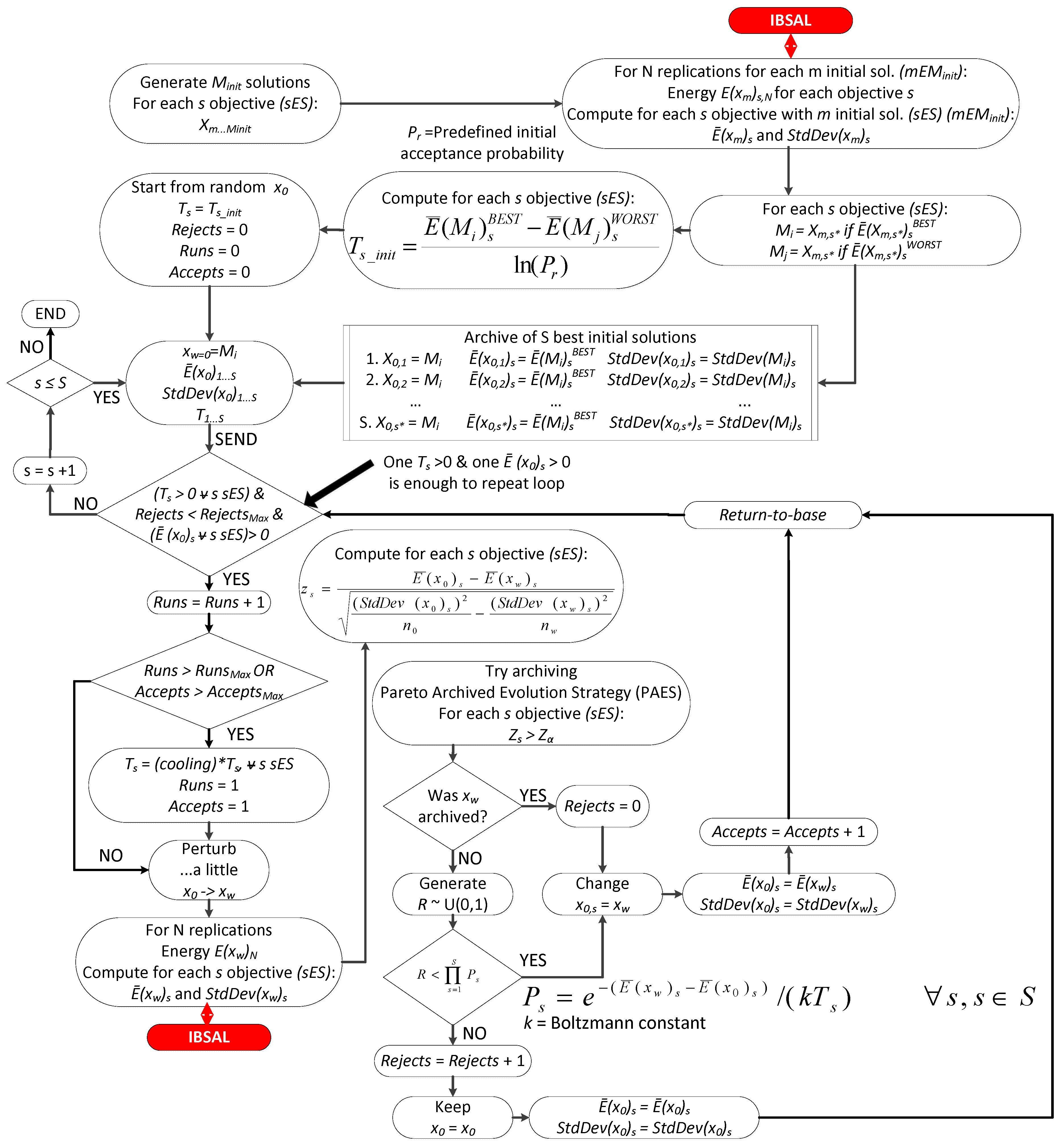
The IBSAL-SimMOpt method is a two-phase procedure that searches a near-optimal set of solutions. During the first phase (i.e., optimization using the SimMOpt) the method is initialized and particular values are given to the decision variables (i.e., perturbed solution). The SimMOpt method uses the Gaussian distribution to perturb the decision variables. A discretization of the Gaussian distribution allows exploring with a high probability those integer values close to the value of the selected variable in the best solution at a given iteration. This perturbation technique is intended to improve the exploitation conditions during local searches. The appropriate selection of the standard deviation improves the exploration conditions. This perturbed solution becomes the input to the IBSAL model during the second phase (i.e., simulation using the extended IBSAL). During the second phase, several replications are computed for evaluating the competing objectives. These evaluations become feedback to a new iteration. Based on these evaluations, a new perturbed solution is computed. This process is repeated until the stopping conditions are met. The stochastic behavior of the system is represented by executing multiple times (i.e., replications) the extended IBSAL model using ExtendSim®™.
The proposed IBSAL-SimMOpt method can be described as follows:
- Extended IBSAL: This research is especially concerned with the costs derived from imperfect quality of feedstock. The IBSAL model is extended so that the cost of imperfect quality of the feedstock is estimated for the corn stover-to-bioethanol SC. For this purpose, blocks were added to the baseline IBSAL for estimating these quality-related costs and other performance measures of interest (e.g., dry matter loss at operations designed to improve the physical characteristics of the feedstock, percentage of moisture, percentage of ash, and probability of having non-conforming stover at the gate of the biorefinery). Extended IBSAL accurately represents the stochastic behavior of elements intervening in the SC and estimates the costs derived from collection, storage, and transportation operations and from having imperfect quality of feedstock.
- SimMOpt: The SimMOpt method is inspired on the procedure used by the stochastic Multi-Objective Simulated Annealing (MOSA). It can be expected that the solutions obtained with this method converge to global optima given the appropriate SA schedule. However, just as with any metaheuristic, optimality is not guaranteed. The procedure can be described as follows:
- (a)
- At the initial iteration, a large set of random solutions is computed. The best solutions for each objective of interest determine a cell in the grid of the Pareto front. The initial temperatures are computed.
- (b)
- Solutions are perturbed and several replications of the evaluation of the objectives are computed. This part is where the extended IBSAL connects with the SimMOpt. The extended IBSAL model is used to perform the replication and return the evaluations of the performance measures to the SimMOpt.
- (c)
- The SimMOpt method uses some hypothesis testing techniques and the Pareto Archive Evolution Strategy (PAES) with the evaluations of the performance measures from the extended IBSAL to find good solutions and perturb the solution that will be used in the following iteration.
- (d)
- The procedure is repeated until some conditions are met (e.g., minimum temperature, value of the objectives, maximum number of iterations, maximum number of rejects, and maximum number of accepts).
- The extended IBSAL and the SimMOpt method are coupled (extended IBSAL-SimMOpt) and used to minimize the set of competing objectives.
- Non-dominated solutions and Pareto-optimal fronts constructed from these solutions are obtained for multiple SA schedules for the problem in the case study.
- Performances of the Pareto-optimal fronts are evaluated using the hypervolume indicator approach.
Figure 1 describes at a high level the interaction between the SimMOpt optimization method (FIRST PHASE) and the extended IBSAL model (SECOND PHASE). This figure shows how decision variables are input to the extended IBSAL from the SimMopt optimization method, and how objective evaluations considering these decision variables are input back to the SimMOpt from the replications performed on the extended IBSAL. The six objectives of interest and four types of decision variables considered in the case study are shown in Figure 1. The definitions of all the abbreviations, symbols and variables used in this paper (figures, tables, and equations) are enlisted in Appendix A.
In the case study presented in Section 4, the types of decisions variables are: (1) initial day of harvest; (2) number of day allowed for field drying; (3) wrap the bales (binary variable); and (4) perform air classification operation (binary variable). The first two are manipulated by the SimMOpt method by perturbation with the purpose of reducing the percentage of moisture uniformly. The third is related to an activity designed to reduce dry matter loss after field drying. The fourth is related to an activity intended to reduce the percentage of ash content. One block is added to the extended IBSAL to represent the opportunity cost derived from failing in meeting the ash content specifications at the conversion facility (i.e., ash dockage). Current biorefineries operating at commercial scale have reported losses due to non-flowable poor quality of biomass and penalization fees [24].
The first and second types of decision variables are defined for each “farm land” (i.e., the amount of land that can be harvested based on the windrower capacity) passing through the Shred/Windrow Module in the extended IBSAL. The third type is defined for each bale passing though the Field-Side Storage Module. The fourth is defined for each truckload leaving the last module of the extended IBSAL model.
3.3. Detailed Description of the SimMOpt Optimization Method
The SimMOpt method is based on SA, which is analogous to the metal annealing process [35,36]. Although SA can be considered slow in converging to a global optimum when compared to other metaheuristics [35], it exhibits one extremely desirable feature. Given the appropriate schedule, which implies a slow cooling rate, convergence to a global minimum is ensured in most applications [35,37]. Figure 2 shows the details of the SimMOpt method and points where it connects with the extended IBSAL.
3.4. Extended IBSAL-SimMopt: Quality Related Blocks
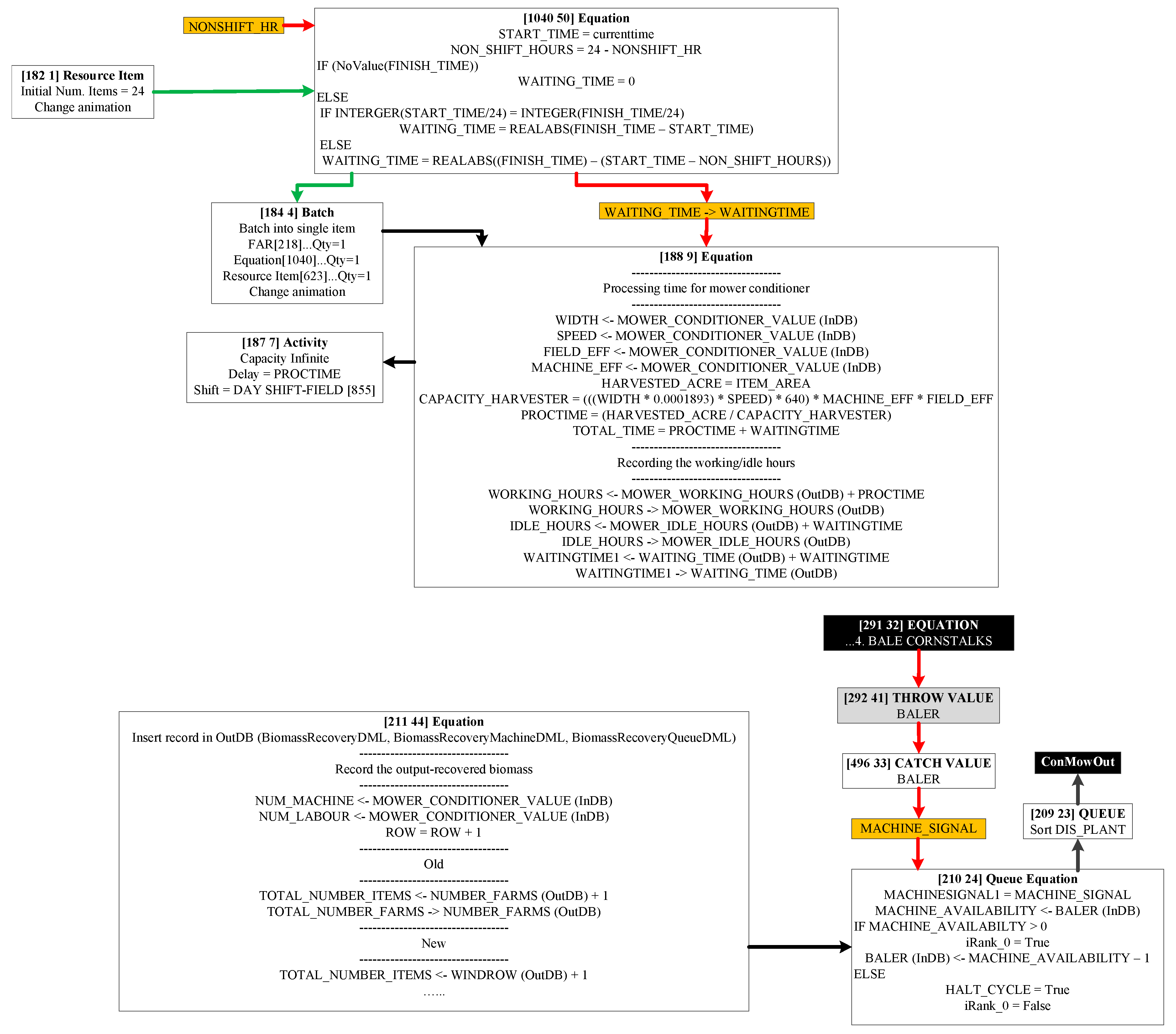
Some elements necessary for the estimation of quality-related costs have been added to the extended IBSAL model. Preliminary versions of the new quality-related blocks were described in [38]. Appendix B shows a diagram block of a section of the original Shred/Windrow Module. The computations performed in the added blocks are discussed in this section.
Initial moisture content of the grain (variable “MoistGrainInit”) (decimal): Moisture content of corn stover after harvest ranges from 35% to 50% when the grain moisture content is at 25%; this level is optimum for harvest. For the case presented by Sokhansanj et al. [7], initial moisture content of stover stalks is assumed at 72% when the grain moisture content is at about 40%. Harvest moisture content of grain at 40% is limited to cold and humid northern regions. In this study, the initial moisture content of grain is assumed to be uniformly distributed (0.35, 0.40) (decimal). Refer to block (83, 24) in the Biomass Field Module—extended IBSAL.
Windrow density (variable “WindrowDensity”) (kg/m2): Khanchi and Birrel [39] evaluate the effect of rainfall and swath density on dry matter, and the composition change during the drying of corn stover. They assume three possible densities 0.8, 1.3, and 2.6 kg/m2 (low density—LD, medium density—MD, and high density—HD, respectively). For this study, the windrow density is assumed to be uniformly distributed (0.8 and 2.6) (decimal). Refer to block (195, 15) in the Shred/Windrow Module—extended IBSAL.
Stover moisture content after harvest (variable “MoistContWet”) (decimal): Moisture content of stover after harvest is determined based on the equations described by Sokhansanj et al. [7]. Refer to block (881, 74) in the Shred/Windrow Module—extended IBSAL.
“RH” and “Temp” depend on “StartDayHarvest”, which is one type of the decision variables that are iteratively evaluated and sent to the extended IBSAL by the SimMOpt optimization tool.
“P(t)” is computed in block [211, 44] in the Shred/Windrow Module—extended IBSAL.
Initial ash content after harvest (variable “AshCont”) (decimal): Schon and Darr [40] enlist the total ash content and all elemental components of ash for the windrowing method and single and multi-pass systems. From the multi-pass bale, this study assumed that the ash content is uniformly distributed (0.08, 0.12). Refer to block [881, 74] in the Shred/Windrow Module—extended IBSAL.
Stover moisture content after field drying (variable “MoistContWet”) (decimal): Moisture content of stover after field drying is determined based on equations described by Khanchi and Birrel [41]. Refer to block [882, 52] in the Shred/Windrow Module—extended IBSAL.
Variable “t” depends on “StartDayHarvest” and “DaysInField”, which are two types of decision variables that are iteratively evaluated sent to the extended IBSAL by the SimMOpt optimization tool.
Ash content after field drying (variable “AshCont”) (decimal): A linear regression was performed on the data provided by Khanchi and Birrel [39]. The resulting equation is used for computing the percentage of ash content after field drying. (Refer to block [882, 52] in the Shred/Windrow Module—extended IBSAL).
Average moisture and ash content (i.e., average “MoistContWet” and “AshCont”) are minimized by two objectives considered during the optimization with the SimMOpt method.
Dry matter loss during field drying (variable “DMLOSS”) (decimal): Linear regression was performed on the data provided by Khanchi and Birrel [39]. The resulting equation is used to compute the percentage of dry matter lost during the field drying period. “0.35” in the numerator of Equation (11) is a multiplier factor used for predicting dry matter loss while biomass is in a “queue” [7,25]. Refer to block [882, 52] in the Shred/Windrow—extended IBSAL.
Items (i.e., farm lands) are delayed in a block a time equal to “DaysInField”.
“WrappingBales” (binary: wrapping/no wrapping): This is the third type of decision variable. It is defined for each bale coming from a particular field. The cost of wrapping each bale is $3/bale and the processing time is 2 min/bale. Bales are delayed in a block during a time equal to the processing time. The dry matter loss percentage for wrapped (“DMLOSSWrap”) bales is 3% [42]. Therefore, if the bales coming from the same farm are wrapped, then The operation of wrapping bales reduces the percentage of dry matter loss. The cost of quality-related operations (“CostQual”) is increased by the cost of wrapping (if applicable). Refer to block [889, 22] in the Field-Side Storage Module—extended IBSAL.
Total cost derived from quality-related operations and amount of dry matter loss (i.e., “CostQual” and “DMLOSS”) are minimized by two objectives considered during the optimization with the SimMOpt method.
“AirClassification” (binary: classification/no classification): This is the fourth type of decision variables. It is defined for each truckload arriving to the conversion facility. The air classification operation is designed to reduce the content of ash. Processing time was assumed to be 3.4 ton/h [43]. The whole ash concentrations in air classified fractions was assumed that corresponding to the 15 Hz light sieve, which results in a uniformly distributed ash content of 6.44 ± 2.54% [43] (i.e., “AshCont” = U(0.0391, 0.0897). Total air classification cost is assumed at $1.05/ton of biomass [43]. The “CostQual” variable is increased accordingly. Refer to block [1267, 120] in the Unload (Facility) Module—extended IBSAL.
“Dockage cost” (CostNoQual): This variable is related to the fifth objective considered during the optimization with the SimMOpt method. This variable is used to compute the cost from having truckloads with bales that have ash content over 5%. These corresponding computations assume that dockage cost is calculated as $1.90/ton for every percentage point of ash above 5% [43]. Refer to block [1262, 114] in the Unload (Facility) Module—extended IBSAL.
In the last block in the last module (i.e., Unload (Facility) Module) in the extended IBSAL, it is possible to identify the items that do not meet the specifications of a maximum of 20% and 5% for the percentage of moisture and ash content, respectively. The minimization of the percentage of items failing to meet these requirements represents the sixth and last objective considered during the optimization. Refer to block [1262, 114] in the Unload (Facility) Module—extended IBSAL.
4. Case Study
The scope of the case study includes field operations, just in time delivery, and storage delivery of corn stover supplied for the production of bioethanol. The starting point of SC under analysis is the “creation of the corn field.” The exit module is the “unload at the biorefinery.” Figure 3 shows the modules of the corn stover SC for the production of bioethanol described in IBSAL for this case study.
Some of the characteristics of the model used in this case study for representing a corn stover SC include: specific dimensions of the geographical implementation, geographical location of the biorefineries, distances from stacking (storage) locations, crop availability and yield, local weather data, fixed biorefinery and storage facility capacities, equipment available for collection and transportation, equipment-related costs (e.g., purchase price, maintenance cost, among others), analytical expressions for the estimation of the residue feedstock delivery price, initial values of the physical characteristics for the corn grain and formulas to compute estimations for the corresponding properties for the stover, and expressions for computing the cost derived from having imperfect feedstock quality in the SC.
4.1. Geographical Regions and Farm Input Data
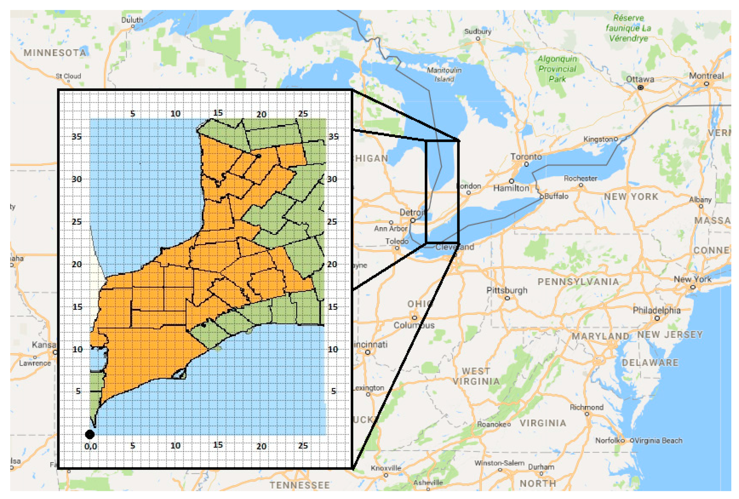
The case study considers 1961 farms distributed in the counties of Lambton, Chatham-kent, Middlesex, and Huron, in the regions of Southern and Western Ontario, Canada. Input information for each farm was entered into IBSAL: size (ac), corn yield (bu/ac), produced corn stover (dry tonne/ac), sustainable corn stover removal (dry tonne/ac), total harvestable corn stover (dry tonne), satellite storage index (zone; only one zone was considered), distance from the satellite storage (km), and distance from the cellulosic sugar plant (km). Figure 4 shows the geographical location of the region considered in the case study.
4.2. Local Weather Input Data
Local weather input data include: daily average temperature (°C), daily snow on the ground (mm), monthly maximum humidity (decimal), monthly minimum humidity (decimal), daily evaporation (mm), daily rainfall (mm), monthly wind speed (m/s) (most common daily wind speed for each month), and monthly average radiation intensity for the hour (watt/m2).
4.3. Machinery Input Data
Table 2 shows the equipment input data provided to the IBSAL model.
4.4. Storage and Other Operational/Quality Input Data
The storage-related input data include the size of bales, stack width (bale), stack height (bale), stack length (bale), clearance between bale stack in a row (ft), clearance between bale stacks in a column (ft), and land charge for storage ($/ac).
Other input data are the daily biomass demand (dry tonne), nutrient replacement cost ($/tonne), daily working hours in the field, and daily working hours performing transportation activities. Input quality-related data consider a user-defined initial moisture content of grain (decimal), and initial ash content (decimal) for the initialization of the simulation model.
4.5. IBSAL Set Up and Tuning
The simulation setup of the extended IBSAL model was determined from literature [7,25]. The “end Time” was set at 8640 h (i.e., one year). The number of replications was set to 30 so it was possible to assume normality (based on the Central Limit Theorem) when performing the hypotheses tests during the optimization phase.
The tuning of the parameters for each SA schedule was determined by using a systematic screening process based on previous experiments with a simplified version of the IBSAL model [38]. Table 3 provides the levels of the parameters corresponding to the SA schedules considered in the screening process. Haddock et al. [35] further discuss the importance of the appropriate setting of these parameters.
5. Results and Discussion
The results from solving the case study by using the IBSAL-SimMOpt method are presented in this section. The solutions are evaluated by using a hypervolume indicator [46] to determine the ability of the model for producing Pareto-optimal fronts.
For schedule (*) it was noted that the percentage of feedstock not meeting the moisture and ash specifications at the conversion process remained constant throughout most of the simulation runs. Therefore, the objective of minimizing this probability was not considered for further analysis.
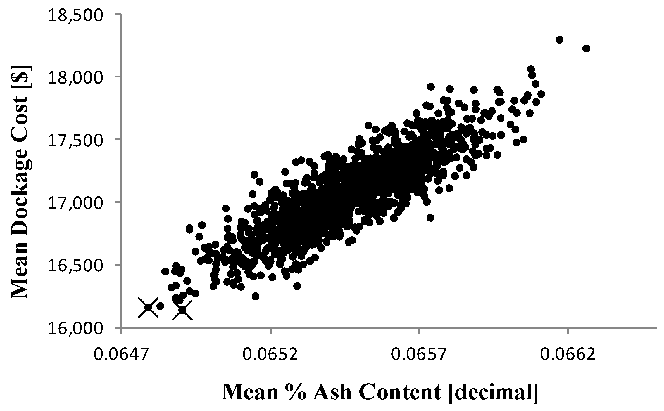
It can be shown that some of the objectives compete with each other, but this is not the case for all objectives under consideration. Some show almost no competition at all. For example, two objectives that change elastically in the same direction are the ash content and the penalization dockage cost. The corresponding Pearson correlation coefficient for the evaluations of the corresponding two objectives using schedule (*) is 0.861. Figure 5 shows the scatter plot of these evaluations. The best solution for each objective is marked with a cross. Other figures in this paper show that not all of objectives behave like this.
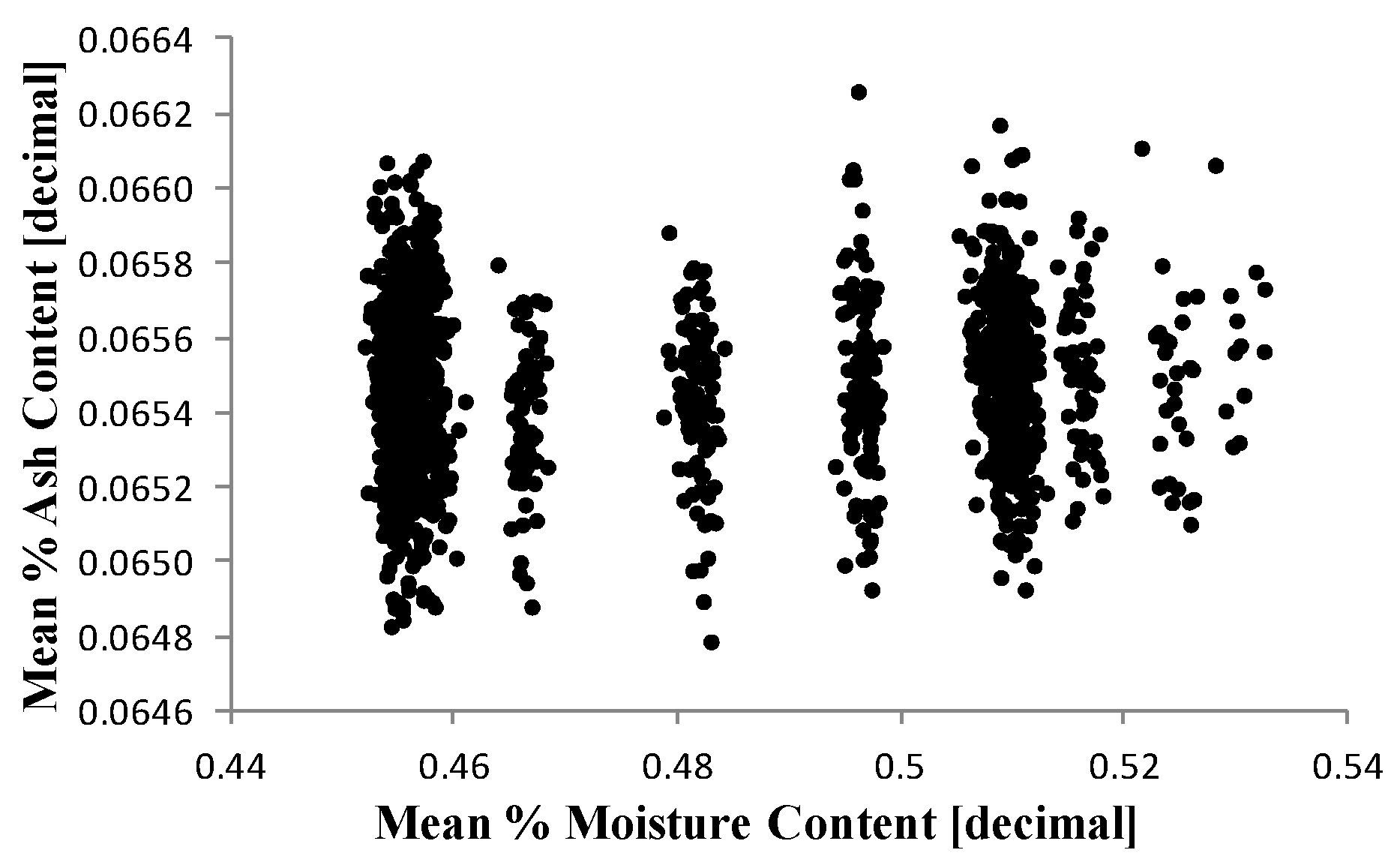
The purpose of the in-field drying operation is to uniformly reduce the percentage of moisture content. In the IBSAL model, the attribute that represents the percentage of moisture content is passed on to the farmlands, and to the bales. These attributes are averaged before forming the batches to be loaded to Stinger®™ equipment, and finally to the truck. This process results in values of this attribute uniformly distributed within a small range about values that depends on the harvest day and the number of days that the stover is left on the field to dry. In this case study, the initial moisture content after harvest is uniformly distributed with values close to 73% (Equation (4)). In Figure 6, Figure 7 and Figure 8, it can be observed that this value is brought down by performing operations designed to improve the physical properties of feedstock to values in the range from 45% to 53%.
In Figure 6, the correlation between the two objectives is close to zero. Moisture content depends on the relative humidity and temperature corresponding to the harvesting day and number of days the stover is left in the field (Equations (1) and (6)–(8)). In addition, dry matter loss depends on the amount of rainfall (Equation (11)). Due to lack of weather data for the region, the relative humidity was averaged for the entire month, while the rainfall was allowed to fluctuate during the month. This caused different moisture contents for fixed values of dry matter loss. Similarly, the percentage of ash depends on the amount of rainfall (Equation (10)). In Figure 8, the correlation between the average moisture content and average ash content is also close to zero.
The IBSAL computes the total tons (fraction of ton) per bale as follows (Refer to block [318, 11] in the Bale Module—extended IBSAL:
Similar formulas are used to compute the tonnage per farm land (Refer to block [195, 14] in the Shred/Windrow Module). Notice that larger values for moisture content result in more tons of dry matter per item (e.g., bales). This relation explains the behavior shown in Figure 7.
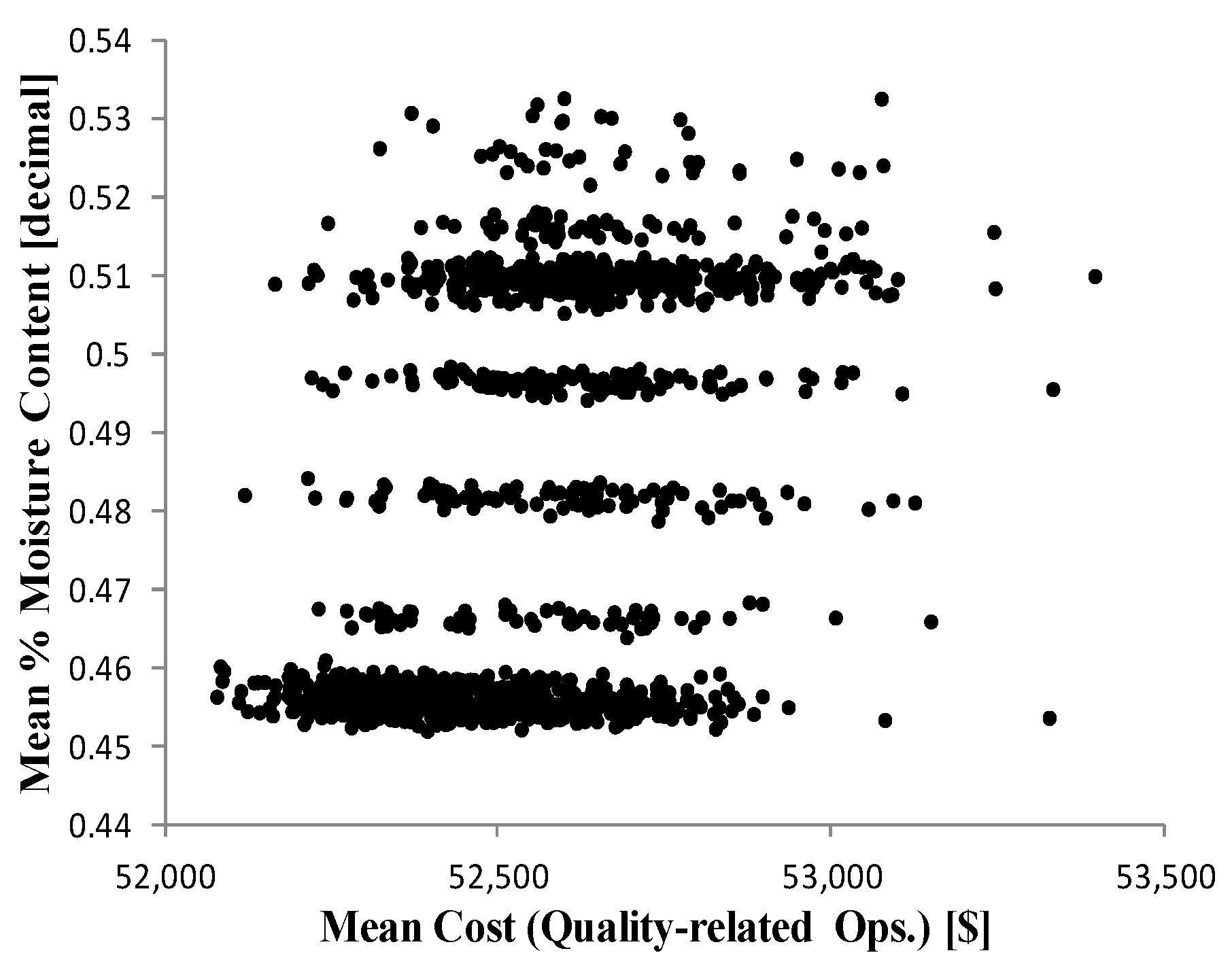
In Figure 7, the corresponding Pearson correlation coefficient is 0.3921. The cost derived from quality-related operations is computed from two sources: (1) the cost from wrapping bales; and (2) the cost from air classifying the truckloads. These costs increase with the number of bales, and tonnage per truckload, respectively. This is supported by the results from IBSAL. These results show that the cost derived from performing quality-related operations has a slight overall positive correlation with moisture content (Figure 7). However, selecting the non-dominated solutions for these objectives implies some trade-offs. Incurring low cost performing operations intended to improve quality results in high moisture content (Figure 9f).
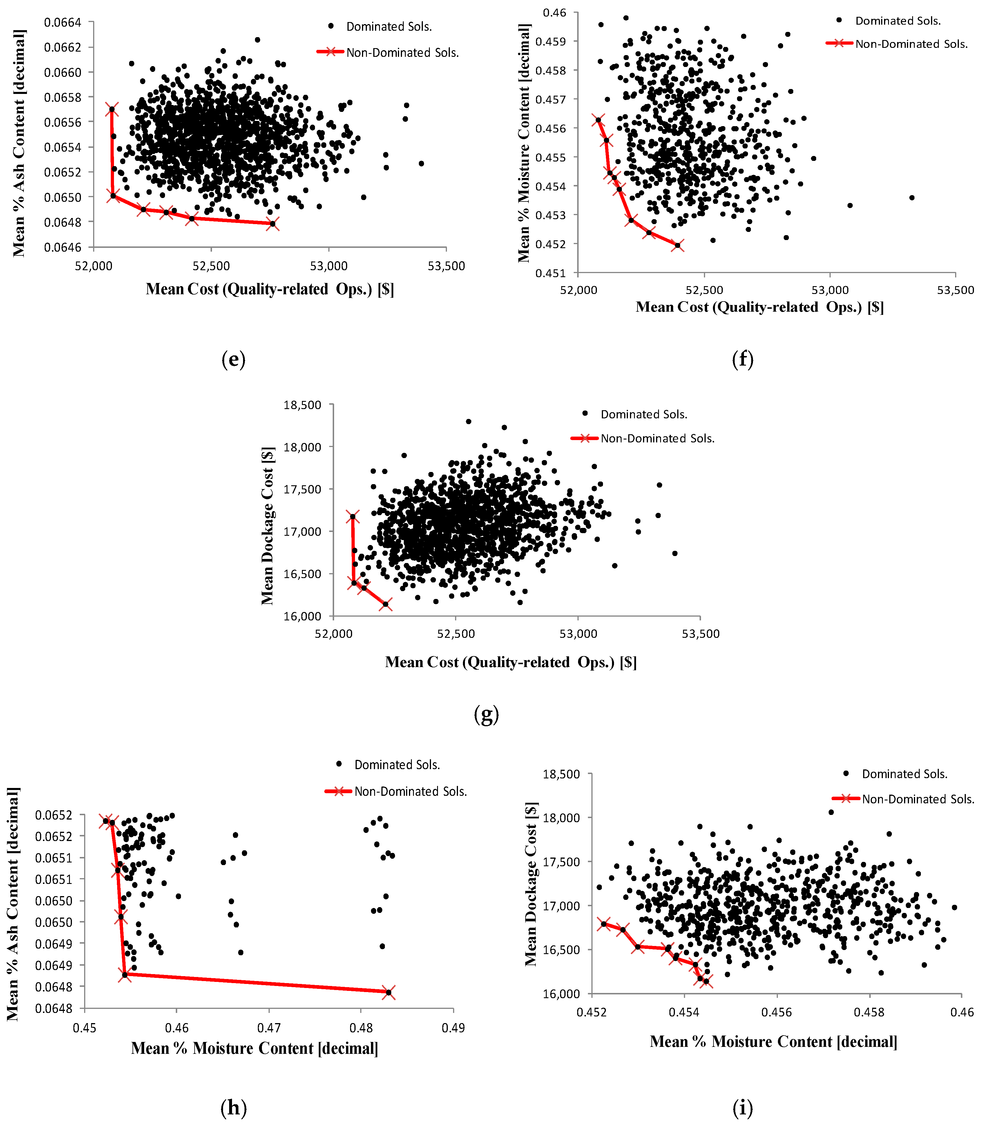
For any pair of objectives in Figure 6, Figure 7 and Figure 8, no single solution optimizes both objectives. Figure 9b,f,h shows the Pareto-optimal fronts for pairs of objectives corresponding to Figure 6, Figure 7 and Figure 8, respectively. The remaining Pareto-optimal fronts for objective pairs are also show in Figure 9.
From the total of computed non-dominated solutions, 31 appeared in one out of the nine fronts (Figure 9), 10 solutions appeared in two, six solutions were present in three, and one solution is included in four. The IBSA-SimMOpt method computed 1366, 94, and 382 solutions using schedules (*), (**), and (***), respectively.
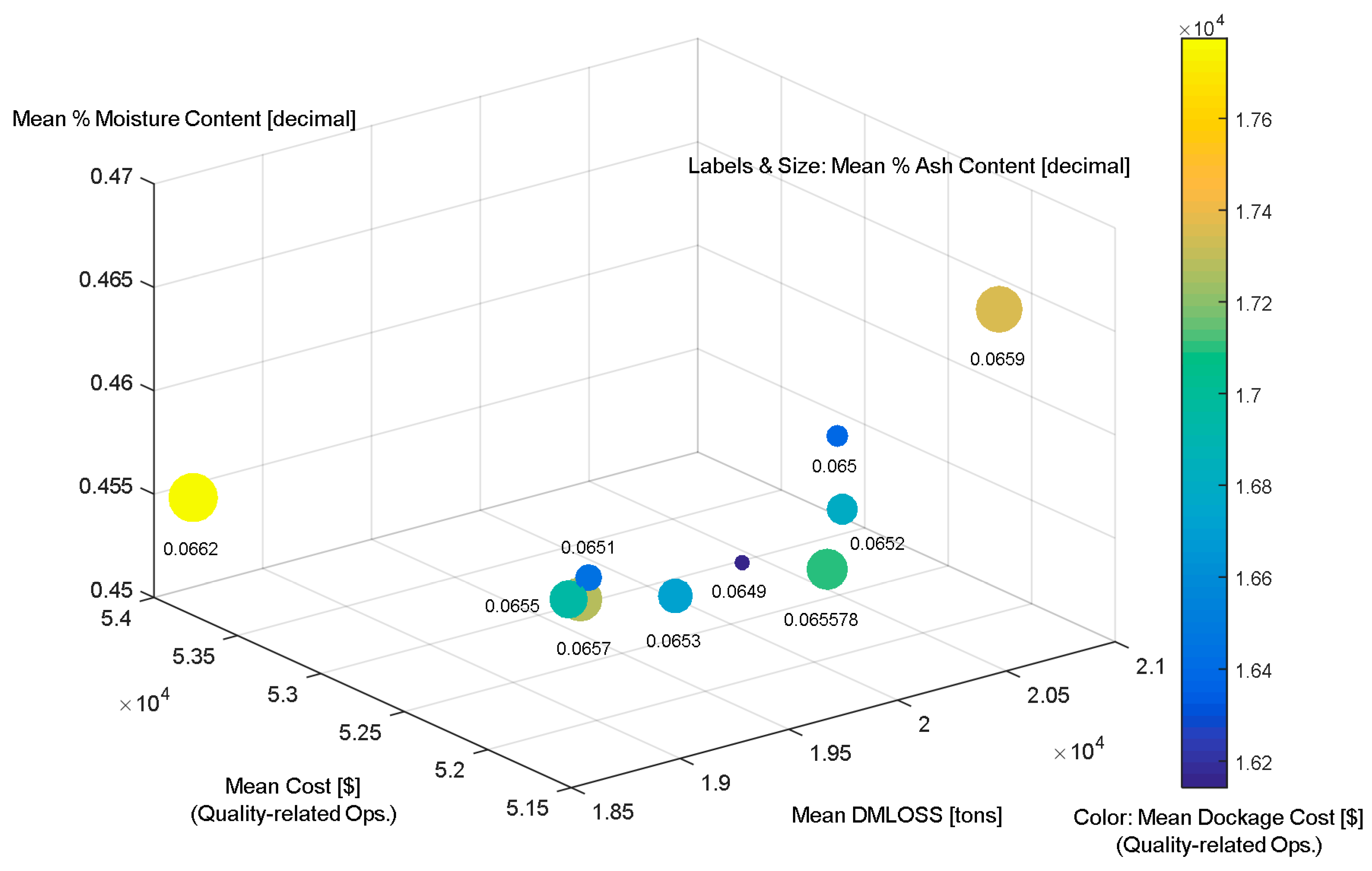
Not all of the non-dominated solutions shown in Figure 9 remain non-dominated solutions when considering the multi-objective problem (i.e., Many-objective Pareto-optimal front). Figure 10 shows the set of non-dominated solutions for the many-objective problem. It can be observed that no single solution (i.e., point) yields minimum values for all objectives. Implementation of any one particular solution from the set depends on the preferences of the decision-maker.
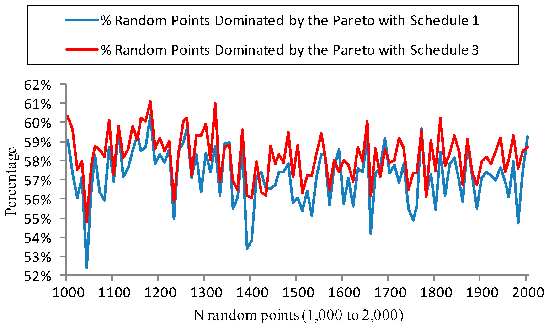
The hypervolume indicator approach [46] is used to compare the performance of the three schedules. Figure 11 shows the hypervolume indicators for the two schedules with the higher values. The random points are computed using a uniform distribution between the minimum values of the objectives from all the computed solutions (mapped onto a space bounded by axes (0, 1)) and 1. Of course, not all the random points represent feasible solutions. For example, the point where all objectives reach their minimum is not feasible as the objectives compete with each other during the optimization. Even when not all the random points represent feasible solutions, this method provides an estimator of the space where inhabiting points are dominated by a given Pareto front. This method allows the quality of the solutions, obtained from using multiple schedules, to be compared.
According to the hypervolume indicators, schedule 3 (i.e., schedule (***)) outperformed the other two. By using this schedule, it is possible to construct a Pareto front with a greater probability of containing solutions that dominate random solutions. For example, for the experiment where 1390 random solutions (not necessarily all feasible) were generated, the non-dominated solutions obtained with schedule (***) outperformed over 56% (779 out of the 1390 random solutions) of them. Solutions from using schedule (**) only outperformed 53.5%. This difference may not seem significant, but the same conclusion can be reached from over a hundred different experiments. Moreover, the difference becomes greater in several experiments.
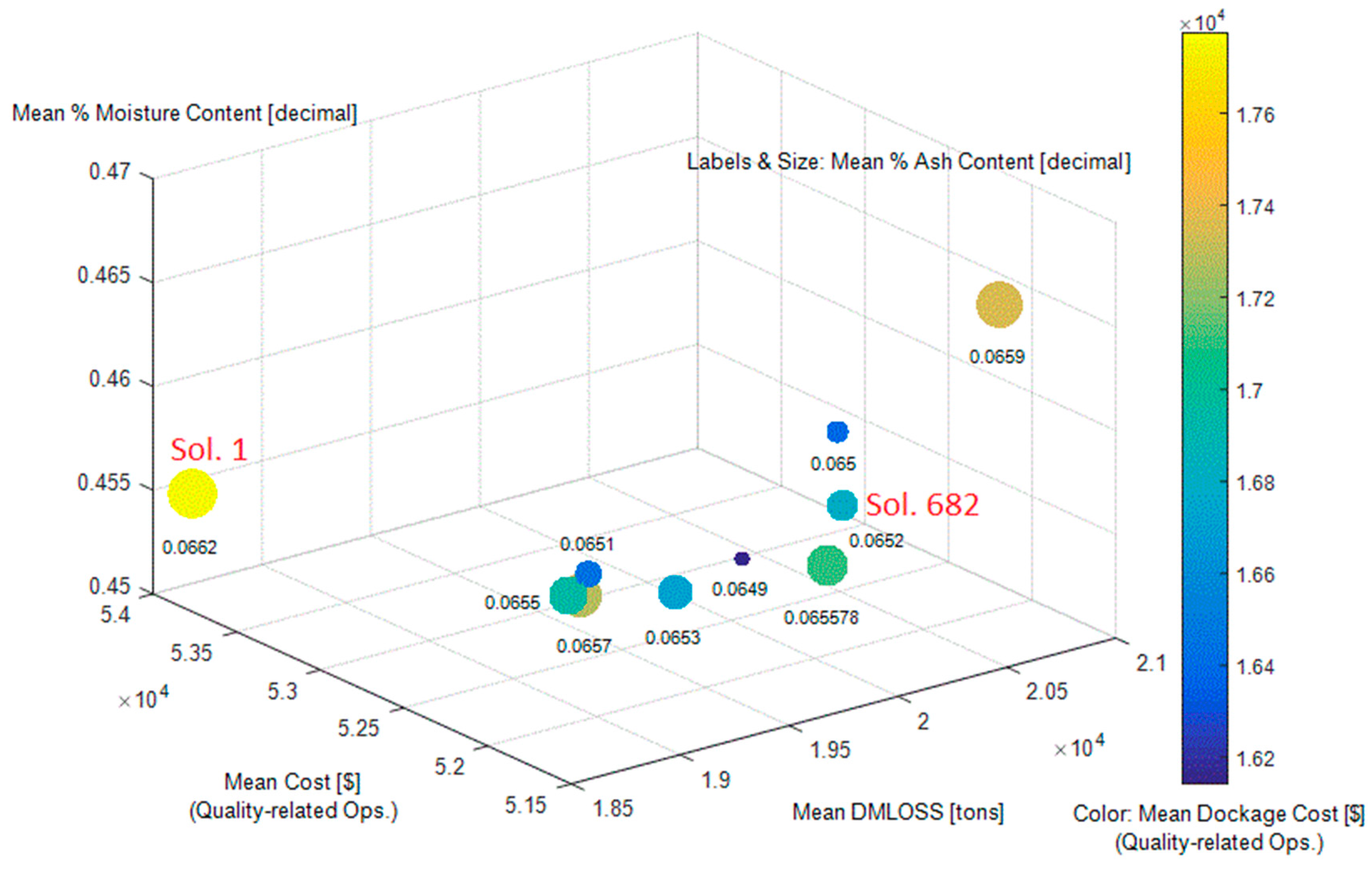
The practitioner is provided with a set of non-dominated solutions. These solutions become more or less attractive depending on the priorities determined by the decision-maker. For example, let us assume that the decision-maker is interested in the following objectives: (1) minimization of the cost derived from implementing activities intended to improve physical characteristics of the feedstock (i.e., moisture content and ash content); (2) minimization of dry matter loss; and (3) minimization of the percentage of moisture content. For illustration purposes, two solutions from the set of non-dominated solutions for the many-objective optimization are compared (Figure 12).
Solution 1 implies that only 8.8% of the farm lands were left on the field for drying for five or more days. This solution resulted in an average moisture content of 45.44%. Solution 682 implies that 10.48% of the farm lands were left on the field for five or more days. The corresponding average moisture content remained close to 45%. However, the trade-off between solutions becomes more evident when the mean cost and the mean DMLOSS objectives are analyzed.
Solution 1 implies an average cumulative cost from quality-related operations of approximately $54,000. Solution 682 implies an average cumulative cost of approximately $52,000. Although the difference is modest, the reduction in dry matter loss from investing more resources on wrapping bales and air separating matter is equal to 2099 tons (solution 1).
Dockage cost is elastic with respect to the percentage of ash content. Even when the average percentage of ash content is similar for solutions 1 and solutions 682, the difference between the dockage costs is proportionally greater. Ash content is computed as the average from all the truckloads at the gate of the conversion facility while the dockage cost is computed as the cumulative cost (see Section 3). It is expected that the dockage cost increases as the ash content increases. However, for small increments on the average ash content, it is possible to observe dockage costs that differ considerably. This is also explained by the fact that dockage cost is affected by the mass at the gate of the biorefinery, and consequently by the cumulative dry matter loss.
The characteristics of the workstations used to run the experiments can set limitations on the size of the instances that can be solved by the proposed method. The equipment used for executing experiments is a computer with an Intel(R)®™ CORE®™ i7-3632QM central processing unit (CPU) processor that operates at 2.20 GHz with 8 GB of random access memory (RAM). The extended IBSAL model was modified and executed using Imagine That! Inc.®™ ExtendSim®™ 9 advanced technology (AT). The SimMOpt method was coded using Microsoft®™ (MS) Excel VBA®™.
6. Conclusions
The IBSAL-SimMOpt method provides the bioenergy industry with a tool capable of finding near-optimal solutions to a set of competing objectives, such as: minimization of dry matter loss, moisture content, ash content, costs related to different operations along the SC (e.g., collection, storage, and transportation), and cost derived from having imperfect quality of feedstock while accurately representing the stochastic behavior of the corn stover supply chain for the production of bioethanol. This provided without the need for additional assumptions intended to simplify the modeling of such complex system.
However, the validity of the model as a representation of the real SC is highly dependent on the assumptions related to the input parameters. These parameters attempt to represent, with numeric values and probability distributions, the behavior of elements interacting in the supply chain. Therefore, it is important to perform the corresponding statistical tests to evaluate the accuracy of these parameters. In the future, the equations included in the new blocks added to IBSAL will be validated using data obtained from field experiments and performing the appropriate statistical tests.
The quality of the solutions can be assessed by computing the hypervolume indicator for the Pareto-optimal solutions obtained from using different methods or settings of a particular method. Results show that the quality of the set of non-dominated solutions depends on the SA schedule. Therefore, it is important in real-life applications to allocate time for the execution of the trial runs required for the tuning of the parameters that define the schedule.
The applicability of the IBSAL-SimMOpt method to real biomass SCs largely depends on the computational effort (i.e., time and data resources) required for the execution of the model. The IBSAL-SimMOpt method required considerably large execution time for solving the problem in the case study. The computational time required by using the three schedules mentioned in Section 5 ranged from four hours to over 48 h. Future work involves quantifying the range of problem sizes that can be solved within reasonable time.
The main contributions of the extended IBSAL-SimMOpt method to biomass SC modeling can be summarized by the following:
- Provides a novel method for finding near-optimal solutions to the problem of designing biomass supply chains that improve the physical characteristics of the feedstock at an acceptable cost.
- Provides the bioenergy sector and the research community with a simulation-based optimization model with activity-based costing that is capable of representing the stochastic behavior of some elements intervening in the corn stover SC for the production of bioethanol. This analytical model can be used for decision making as well as educational and training purposes since it allows the user to conduct “what if” scenarios.
- Optimizes a set of competing individual objectives that include the cost of having imperfect corn stover quality for the production of bioethanol. The bioenergy industry will potentially benefit from this methodology, which can be adapted to minimize multiple costs in the biomass supply chain (e.g., collection, storage, transportation, and quality-related) as well as other key output measurements (e.g., dry matter loss, moisture content, and ash content) within a computational effort that is sensible for the solution of real problems. Here, the decision maker assigns the priority of objectives when finding a solution.
- Allows modeling complex systems with multiple intertwined stochastic elements; this is one of the most powerful features. The IBSAL-SimMOpt method captures the variability in the behavior of the elements of the biomass SC. Replications of the IBSAL model are performed to represent the stochastic behavior of the system.
- The SimMOpt method interacts with the output from the extended IBSAL model. There are no limitations in terms of the characteristics of the equalities/inequalities representing the objectives and constraints, which is an important concern when using mathematical programming instead of simulation.
- The IBSAL-SimMOpt method can be modified with relative ease using a top-down or bottom-up approach, as required. Therefore, the method can be easily transferred to applications involving biomass SCs with a wider range of feedstock to larger instances.
Acknowledgments
Funding for this research was provided by the U.S. Department of Energy, Office of Energy Efficiency and Renewable Energy, Bioenergy Technologies Office (4000142556). This material is based upon work that is supported by the National Institute of Food and Agriculture, U.S. Department of Agriculture, under award number 2014-38502-22598 (OK State Sub # 3TC460, 2568930.UTSA1) through South Central Sun Grant Program and the Hispanic-Serving Institutions (HSI) program (2015-38422-24064). The fellowship from the Mexican Council for Science and Technology (CONACYT) is gratefully acknowledged. The support provided by Imagine That!®™ by donating of a full version of ExtendSim®™ through the ExtendSim Research Grant is gratefully acknowledged. The research work on the IBSAL model by Sokhansanj, Turhollow, and Ebadian was relevant for the development of the proposed approach.
Author Contributions
Hernan Chavez developed the IBSAL-SimMOpt solution procedure and solved the instance of the extended IBSAL model. Krystel K. Castillo-Villar supervised and provided theoretical and conceptual advice. Erin Webb provided expert advice on biomass SC and the baseline IBSAL model.
Conflicts of Interest
The authors declare no conflict of interest. This manuscript has been authored by University of Tennessee (UT)-Battelle, Limited Liability Company (LLC) under Contract No. DE-AC05-00OR22725 with the U.S. Department of Energy. The United States Government retains and the publisher, by accepting the article for publication, acknowledges that the United States Government retains a non-exclusive, paid-up, irrevocable, worldwide license to publish or reproduce the published form of this manuscript, or allow others to do so, for United States Government purposes. The Department of Energy (DoE) will provide public access to these results of federally sponsored research in accordance with the DoE Public Access Plan (http://energy.gov/downloads/doe-public-access-plan). The founding sponsors had no role in the design of the study; in the collection, analyses, or interpretation of data; in the writing of the manuscript, and in the decision to publish the results.
Appendix A
| Symbols | |
| S | Set of objective |
| M | Set of solutions |
| Xm | Solution m (m M) |
| E(Xm)s | Evaluation of objective s by considering solution m (s S, m M) |
| Ts | Temperature related to objective s (s S) |
| NBi | The i-th return-to-base occurs after these many iterations |
| N | Set of replications |
| Minit | Set of initial solutions |
| W | Set of computed solutions |
| Xm | Solution m (m Mini) |
| Mi = Xm,s* | Best initial solution for objective s (m Minit, i Minit, s S) |
| Mj = Xm,s* | Worst initial solution for objective s. (m Minit, j Minit, s S) |
| xw | Solution w computed by a series of perturbations starting from Mi (w W) |
| E(Xw)s | Evaluations of objective s by considering solution Xw (s S, w W) |
| Ts_init | Initial temperature |
| Ts | Temperature |
| Ē(Xw)s | Mean value from evaluations of objective s by considering solution Xw (s S, w W) |
| StdDev(Xw)s | Standard deviation from evaluations of objective s by considering solution Xw (s S, w W) |
| Runsmax | Maximum number of runs (SA schedule) |
| Rejectsmax | Maximum number of rejects (SA schedule) |
| Acceptsmax | Maximum number of accepts (SA schedule) |
| zs | Critical value (Hypotheses testing on the mean of evaluations of objective s for two large samples) (s S) |
| nw | Size of sample consisting of the evaluations of objectives while considering solution Xw (w W) |
| zα | Value from standard normal table corresponding to significance level α. |
| R | Pseudo-random number ~Uniform(0, 1) |
| Ps | Probability of acceptance of solution Xw based on the mean of the evaluations of objective s (s S) |
| K | Boltzmann constant |
| Sched. | SA Schedule |
| Pr | Probability of acceptance of neighbor solution |
| MinTemp | Minimum Temperature—stopping criterion |
| MinOFVal | Minimum value of the objective evaluation—stopping criterion |
| Ali | Number of solutions in the candidate list from which a solution is selected when the SimMOpt returns-to-base |
| Lm | Zero dry matter loss (due to machine) at 80% moisture content |
| Lmmax | Machine biomass loss (decimal) |
| MoistContWet | Moisture content in stover (decimal) |
| Mwmax | Moisture content with zero machine loss (decimal wb) |
| DMLoss | Loss tonnage due to machine (tonne) |
| ItemTom | Tonnage of item (e.g., land) |
| MoistGrainInit | Initial moisture content of the grain (decimal) |
| WindrowDensity | Windrow density (kg/m2) |
| MoistEq(t) | Equilibrium moisture content on the grain (cob) at time t (decimal) |
| RH(t) | relative humidity at time t (decimal) |
| Temp(t) | Ambient air temperature at time t (°C) |
| P(t) | Cumulative harvested fraction at time t (decimal) |
| CumHarvestAreaDay | Cumulative harvested area (considered for all farm lands harvested on the same day) (ac) |
| MoistGrainWet(t) | Grain kernel moisture content at time t (decimal). Assumed ≥ 0.08 |
| MoistContWet | Moisture content of the stover stalk (w.b.) (decimal) |
| Mo | Initial moisture content (decimal) |
| Me | Equilibrium moisture calculated by modified Oswin equation (decimal) |
| K | Drying rate constant (applies to Equations (8) and (9)) |
| AvgRH(t) | Average relative humidity at time t (decimal) |
| VPD(t) | Vapor pressure density at time t |
| Rad(t) | Radiation intensity for the hour at time t (watt/m2) |
| WS(t) | Wind speed at time t (m/s) |
| T | Each day the stover is left on the field for dying (days) |
| StartDayHarvest | Start day of harvest (type of decision variable) |
| DaysInField | Number of days left on the field for drying (type of decision variable) |
| AshCont | Ash content after field drying (decimal) |
| Rainfall(t) | Amount of rain at time t (mm) |
| DMLOSS | Dry matter loss during field drying (decimal) |
| WrappingBales | Binary: wrapping/no wrapping (type of decision variable) |
| DMLOSSWrap | Dry matter loss percentage for wrapped bales (decimal) |
| CostQual | Cost of quality-related operations ($) |
| AirClassification | Binary: classification/no classification |
| CostNoQual | Dockage cost ($) |
| Abbreviations | |
| IBSAL | Integrated Biomass Supply Analysis and Logistics |
| SimMOpt | Simulation-based Multi-Objective Optimization |
| SA | Simulated Annealing |
| NREL | National Renewable Energy Laboratory |
| DES | Discrete Events Simulation |
| SC | Supply Chain |
| ORNL | Oak Ridge National Laboratory |
| DoE | Department of Energy |
| MP | Mathematical Programming |
| QP | Quadratic Programming |
| PROMETHEE | Preference Ranking Organization Method for Enrichment of Evaluations |
| MILP | Mixed-Integer Linear Programming |
| BLM | Biomass Logistic Model |
| FS | Feedstock Supply |
| IBSAL-MC | IBSAL Multi-Crop |
| SD | Systems Dynamics |
| MOSA | Multi-Objective Simulated Annealing |
| PAES | Pareto Archive Evolution Strategy |
| CTL | Central Limit Theorem |
| w.b. | Wet Basis |
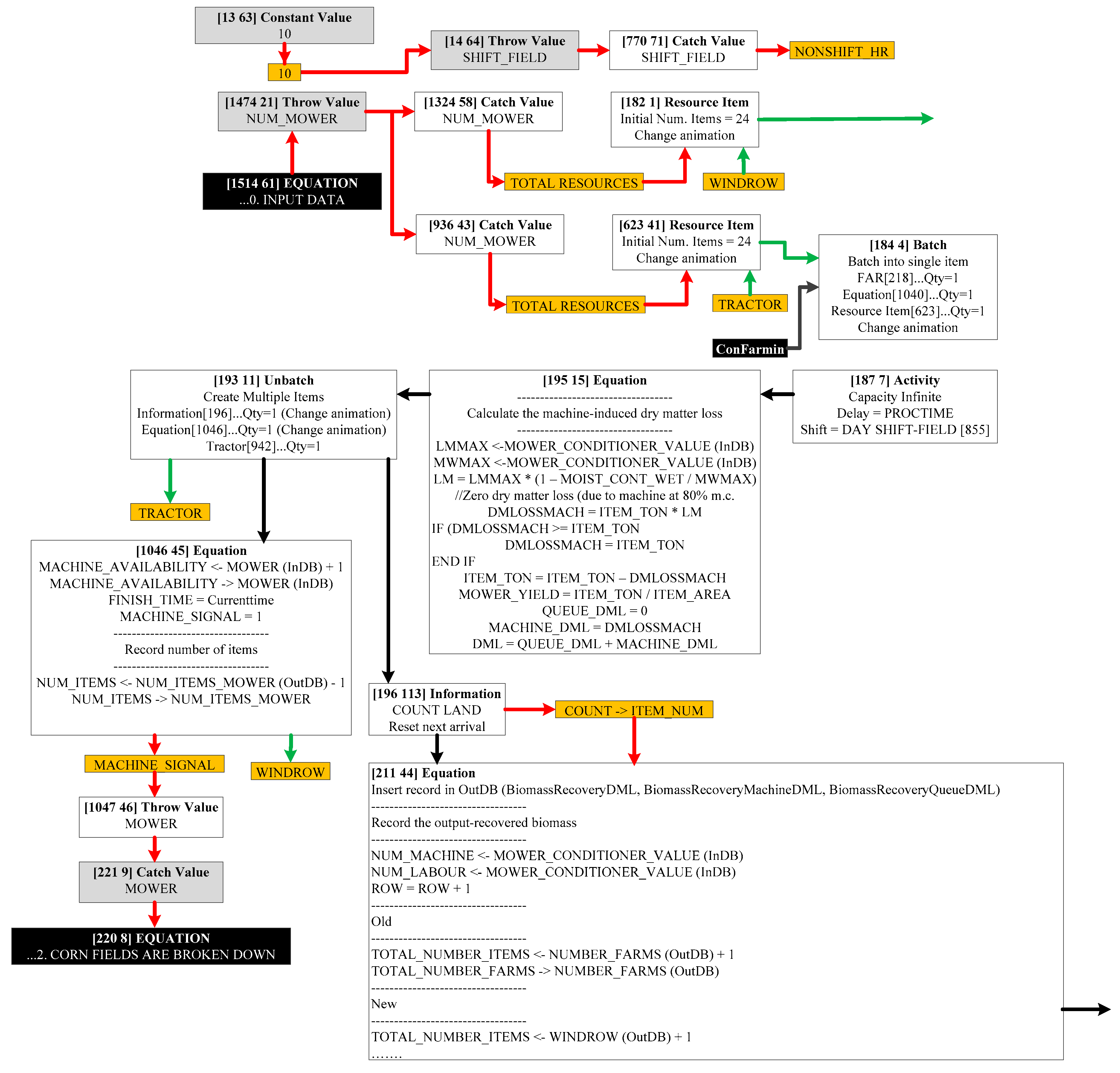
Appendix B
Figure A1.
Section of the original Shred/Windrow module.

References
- Office of Energy Efficiency & Renewable Energy. Available online: http://www.energy.gov/eere/bioenergy/biomass-feedstocks (accessed on 2 August 2017).
- Langholtz, M.H.; Stokes, B.J.; Eaton, L.M. 2016 Billion-Ton Report: Advancing Domestic Resources for a Thriving Bioeconomy, Volume 1: Economic Availability of Feedstocks; Oak Ridge National Laboratory: Oak Ridge, TN, USA, 2016.
- Caputo, A.C.; Palumbo, M.; Pelagagge, P.M.; Scacchia, F. Economics of biomass energy utilization in combustion and gasification plants: Effects of logistic variables. Biomass Bioenergy 2015, 28, 35–51. [Google Scholar] [CrossRef]
- Leistritz, F.L.; Hodur, N.M.; Senechal, D.M.; Stowers, M.D.; McCalla, D.; Saffron, C.M. Biorefineries Using Agricultural Residue Feedstock in the Great Plains. Available online: http://ageconsearch.umn.edu/bitstream/7323/2/ae070001.pdf (accessed on 2 August 2017).
- Sadhukhan, J.; Ng, K.S.; Hernandez, E.M. Biorefineries and Chemical Processes: Design, Integration and Sustainability Analysis; John Wiley & Sons: Hoboken, NJ, USA, 2014. [Google Scholar]
- Stephen, J.D. Biorefinery Feedstock Availability and Price Variability: Case Study of the Peace River Region, Alberta. Ph.D. Thesis, University of British Columbia, Vancouver, BC, Canada, 2008. [Google Scholar]
- Sokhansanj, S.; Kumar, A.; Turhollow, A.F. Development and implementation of integrated biomass supply analysis and logistics model (IBSAL). Biomass Bioenergy 2006, 30, 838–847. [Google Scholar] [CrossRef]
- Aslam, T.; Amos, H.N. Multi-objective optimization for supply chain management: A literature review and new development. In Proceedings of the 2010 8th International Conference on Supply Chain Management and Information Systems (SCMIS), Hong Kong, China, 6–8 October 2010; pp. 1–8. [Google Scholar]
- Kumar, A.; Sokhansanj, S.; Flynn, P.C. Development of a multicriteria assessment model for ranking biomass feedstock collection and transportation systems. Appl. Biochem. Biotechnol. 2006, 129, 71–87. [Google Scholar] [CrossRef]
- Kumar, A.; Sokhansanj, S. Switchgrass (Panicum vigratum, L.) delivery to a biorefinery using integrated biomass supply analysis and logistics (IBSAL) model. Bioresour. Technol. 2007, 98, 1033–1044. [Google Scholar] [CrossRef] [PubMed]
- Ravula, P.P.; Grisso, R.D.; Cundiff, J.S. Cotton logistics as a model for a biomass transportation system. Biomass Bioenergy 2008, 32, 314–325. [Google Scholar] [CrossRef]
- Stephen, J.; Sokhansanj, S.; Bi, X.; Sowlati, T.; Kloeck, T.; Townley-Smith, L.; Stumborg, M. The impact of agricultural residue yield range on the delivered cost to a biorefinery in the Peace River region of Alberta, Canada. Biosyst. Eng. 2010, 105, 298–305. [Google Scholar] [CrossRef]
- Sokhansanj, S.; Mani, S.; Tagore, S.; Turhollow, A. Techno-economic analysis of using corn stover to supply heat and power to a corn ethanol plant–Part 1: Cost of feedstock supply logistics. Biomass Bioenergy 2010, 34, 75–81. [Google Scholar] [CrossRef]
- An, H.; Wilhelm, W.E.; Searcy, S.W. A mathematical model to design a lignocellulosic biofuel supply chain system with a case study based on a region in Central Texas. Bioresour. Technol. 2011, 102, 7860–7870. [Google Scholar] [CrossRef] [PubMed]
- Shastri, Y.N.; Rodriguez, L.F.; Hansen, A.C.; Ting, K. Impact of distributed storage and pre-processing on Miscanthus production and provision systems. Biofuels Bioprod. Biorefining 2012, 6, 21–31. [Google Scholar] [CrossRef]
- An, H.; Searcy, S.W. Economic and energy evaluation of a logistics system based on biomass modules. Biomass Bioenergy 2012, 46, 190–202. [Google Scholar] [CrossRef]
- Larasati, A.; Liu, T.; Epplin, F.M. An analysis of logistic costs to determine optimal size of a biofuel refinery. Eng. Manag. J. 2012, 24, 63–72. [Google Scholar] [CrossRef]
- Ebadian, M.; Sowlati, T.; Sokhansanj, S.; Smith, L.T.; Stumborg, M. Development of an integrated tactical and operational planning model for supply of feedstock to a commercial-scale bioethanol plant. Biofuels Bioprod. Biorefining 2014, 8, 171–188. [Google Scholar] [CrossRef]
- Igathinathane, C.; Archer, D.; Gustafson, C.; Schmer, M.; Hendrickson, J.; Kronberg, S.; Faller, T. Biomass round bales infield aggregation logistics scenarios. Biomass Bioenergy 2014, 66, 12–26. [Google Scholar] [CrossRef]
- Searcy, S.W.; Hartley, B.E.; Thomasson, J.A. Evaluation of a modular system for low-cost transport and storage of herbaceous biomass. BioEnergy Res. 2014, 7, 824–832. [Google Scholar] [CrossRef]
- Ren, L.; Cafferty, K.; Roni, M.; Jacobson, J.; Xie, G.; Ovard, L.; Wright, C. Analyzing and comparing biomass feedstock supply systems in China: Corn stover and sweet sorghum case studies. Energies 2015, 8, 5577–5597. [Google Scholar] [CrossRef]
- Chávez, H.; Castillo-Villar, K.K.; Herrera, L.; Bustos, A. Simulation-based multi-objective model for supply chains with disruptions in transportation. Robot. Comput. Integr. Manuf. 2017, 43, 39–49. [Google Scholar] [CrossRef]
- Pinho, T.M.; Coelho, J.P.; Moreira, A.P.; Boaventura-Cunha, J. Modelling a biomass supply chain through discrete-event simulation. IFAC PapersOnLine 2016, 49, 84–89. [Google Scholar] [CrossRef]
- Castillo-Villar, K.K.; Minor-Popocatl, H.; Webb, E. Quantifying the impact of feedstock quality on the design of bioenergy supply chain networks. Energies 2016, 9, 203. [Google Scholar] [CrossRef]
- Sokhansanj, S.; Turhollow, A.; Wilkerson, E. Development of the Integrated Biomass Supply Analysis and Logistics Model (IBSAL); Oak Ridge National Laboratory: Oak Ridge, TN, USA, 2008.
- Ebadian, M.; Sowlati, T.; Sokhansanj, S.; Stumborg, M.; Townley-Smith, L. A new simulation model for multi-agricultural biomass logistics system in bioenergy production. Biosyst. Eng. 2011, 110, 280–290. [Google Scholar] [CrossRef]
- De Meyer, A.; Cattrysse, D.; Rasinmäki, J.; Van Orshoven, J. Methods to optimise the design and management of biomass-for-bioenergy supply chains: A review. Renew. Sustain. Energy Rev. 2014, 31, 657–670. [Google Scholar] [CrossRef]
- Diamond, B. The ExtendSim Optimizer; Imagine That Inc.: San Jose, CA, USA, 2003. [Google Scholar]
- Kadam, K.L.; McMillan, J.D. Availability of corn stover as a sustainable feedstock for bioethanol production. Bioresour. Technol. 2003, 88, 17–25. [Google Scholar] [CrossRef]
- Sokhansanj, S.; Mani, S.; Turhollow, A.; Kumar, A.; Bransby, D.; Lynd, L.; Laser, M. Large-scale production, harvest and logistics of switchgrass (Panicum virgatum L.)—Current technology and envisioning a mature technology. Biofuels Bioprod. Biorefining 2009, 3, 124–141. [Google Scholar] [CrossRef]
- Popp, M.P.; Searcy, S.W.; Sokhansanj, S.; Smartt, J.B.; Cahill, N.E. Influence of weather on the predicted moisture content of field chopped energy sorghum and switchgrass. Appl. Eng. Agric. 2015, 31, 179–190. [Google Scholar]
- Kenney, K.L.; Cafferty, K.G.; Jacobson, J.J.; Bonner, I.J.; Gresham, G.L.; Hess, R.J.; Ovard, L.P.; Smith, W.A.; Thompson, D.N.; Thompson, V.S.; et al. Feedstock Supply System Design and Economics for Conversion of Lignocellulosic Biomass to Hydrocarbon Fuels: Conversion Pathway: Biological Conversion of Sugars to Hydrocarbons; Idaho National Laboratory: Idaho Falls, ID, USA, 2013.
- Kenney, K.L.; Smith, W.A.; Gresham, G.L.; Westover, T.L. Understanding biomass feedstock variability. Biofuels 2013, 4, 111–127. [Google Scholar] [CrossRef]
- Bonner, I.J.; Smith, W.A.; Einerson, J.J.; Kenney, K.L. Impact of harvest equipment on ash variability of baled corn stover biomass for bioenergy. BioEnergy Res. 2014, 7, 845–855. [Google Scholar] [CrossRef]
- Haddock, J.; Mittenthal, J. Simulation optimization using simulated annealing. Comput. Ind. Eng. 1992, 22, 387–395. [Google Scholar] [CrossRef]
- Van Laarhoven, P.J.; Aarts, E.H. Simulated annealing. In Simulated Annealing: Theory and Applications; Springer: Dordrecht, The Netherlands, 1987; pp. 7–15. [Google Scholar]
- Geman, S.; Geman, D. Stochastic relaxation, Gibbs distributions, and the Bayesian restoration of images. IEEE Trans. Pattern Anal. Mach. Intell. 1984, 6, 721–741. [Google Scholar] [CrossRef] [PubMed]
- Chavez, H.; Castillo-Villar, K.K.; Webb, E. Simulation-based approach for the optimization of a biofuel supply chain. In Proceedings of the Industrial and Systems Engineering Research Conference (ISERC), Pittsburgh, PA, USA, 20–23 May 2017. [Google Scholar]
- Khanchi, A.; Birrell, S.J. Effect of rainfall and swath density on dry matter and composition change during drying of switchgrass and corn stover. Biosyst. Eng. 2017, 153, 42–51. [Google Scholar] [CrossRef]
- Schon, B.; Matt, D. Corn Stover Ash; Iowa State University: Ames, IA, USA, 2014. [Google Scholar]
- Khanchi, A.; Birrell, S. Drying models to estimate moisture change in switchgrass and corn stover based on weather conditions and swath density. Agric. Forest Meteorol. 2017, 237, 1–8. [Google Scholar] [CrossRef]
- Vadas, P.A.; Digman, M.F. Production costs of potential corn stover harvest and storage systems. Biomass Bioenergy 2013, 54, 133–139. [Google Scholar] [CrossRef]
- Thompson, V.S.; Lacey, J.A.; Hartley, D.; Jindra, M.A.; Aston, J.E.; Thompson, D.N. Application of air classification and formulation to manage feedstock cost, quality and availability for bioenergy. Fuel 2016, 180, 497–505. [Google Scholar] [CrossRef]
- Map Data @ 2017 Google United States. Available online: https://www.google.com/maps/@42.2748687,-82.2910045,7.5z (accessed on 4 April 2017).
- Suppapitnarm, A.; Seffen, K.A.; Parks, G.T.; Connor, A.M.; Clarkson, P.J. Multiobjective optimisation of bicycle frames using simulated annealing. In Proceedings of the 1st ASMO/ISSMO Conference on Engineering Design Optimization, Ilkley, UK, 8–9 July 1999. [Google Scholar]
- Cao, Y. Hypervolume Indicator. Available online: https://www.mathworks.com/matlabcentral/fileexchange/19651-hypervolume-indicator (accessed on 2 August 2017).
Figure 1.
Extended IBSAL-SimMOpt method.
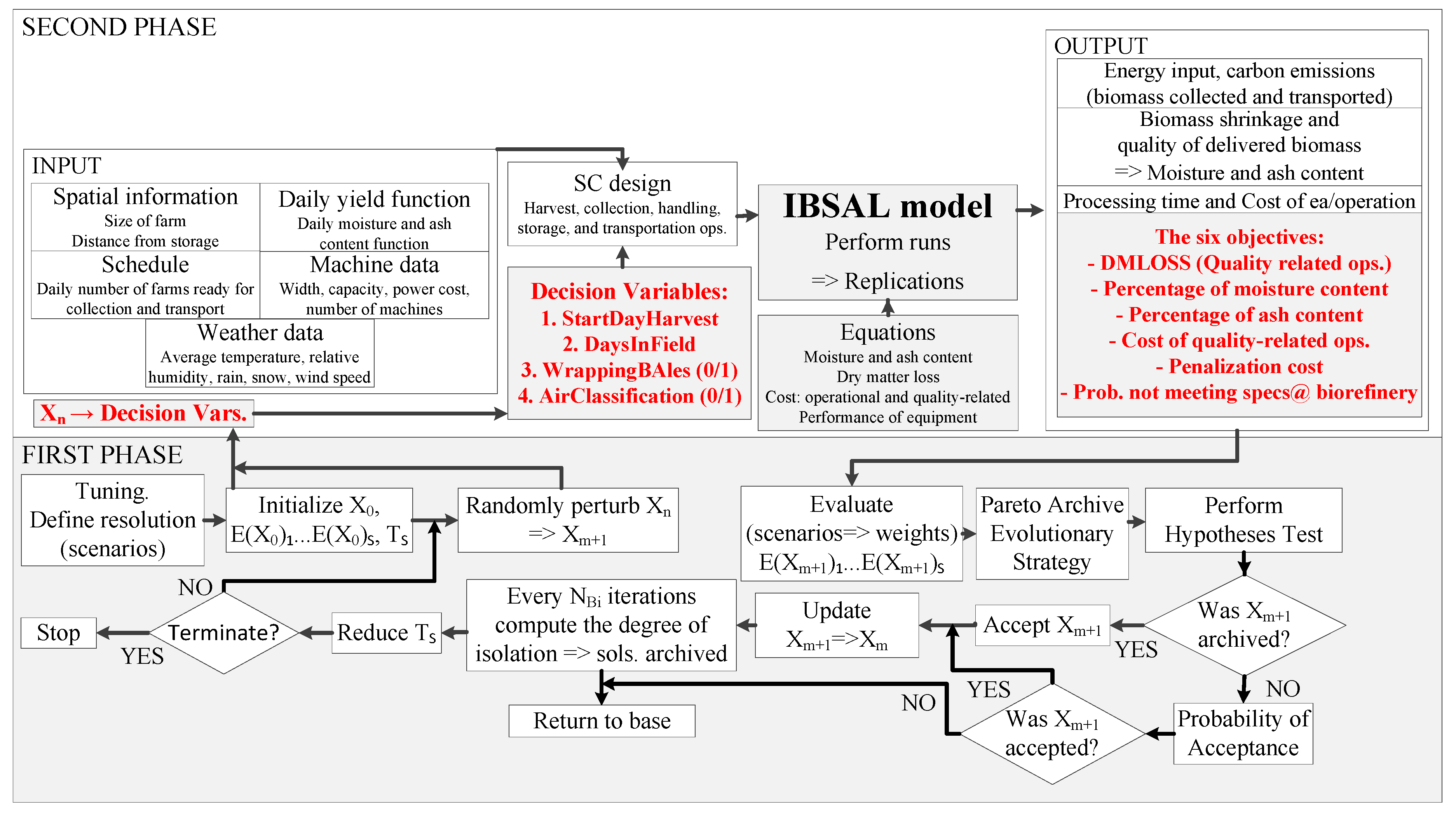
Figure 2.
SimMOpt optimization method.

Figure 3.
Corn stover SC for the production of bioethanol (IBSAL).
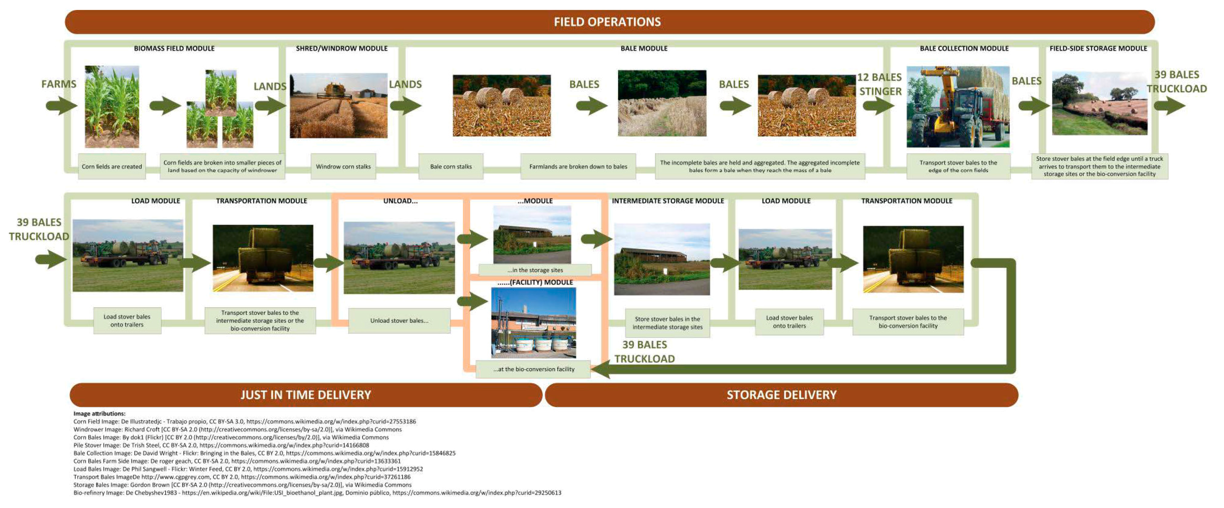
Figure 4.
Geographical location (based on [44]).
Figure 4.
Geographical location (based on [44]).

Figure 5.
Scatter plot percentage of ash content vs. dockage cost (schedule (*)).

Figure 6.
Average MC vs. DMLOSS (schedule (*)).

Figure 7.
Average ash content vs. cost (schedule (*)).

Figure 8.
Average ash content vs. MC (schedule (*)).

Figure 9.
Pareto fronts (schedule (*)): (a) mean DMLOSS vs. mean cost; (b) mean DMLOSS vs. mean percent moisture; (c) mean DMLOSS vs. mean percent ash; (d) mean DMLOSS vs. mean dockage cost; (e) mean cost vs. mean percent ash; (f) mean cost vs. mean percent moisture; (g) mean cost vs. mean dockage cost; (h) mean percent moisture vs. mean percent Ash; and (i) mean dockage cost vs. mean percent moisture.
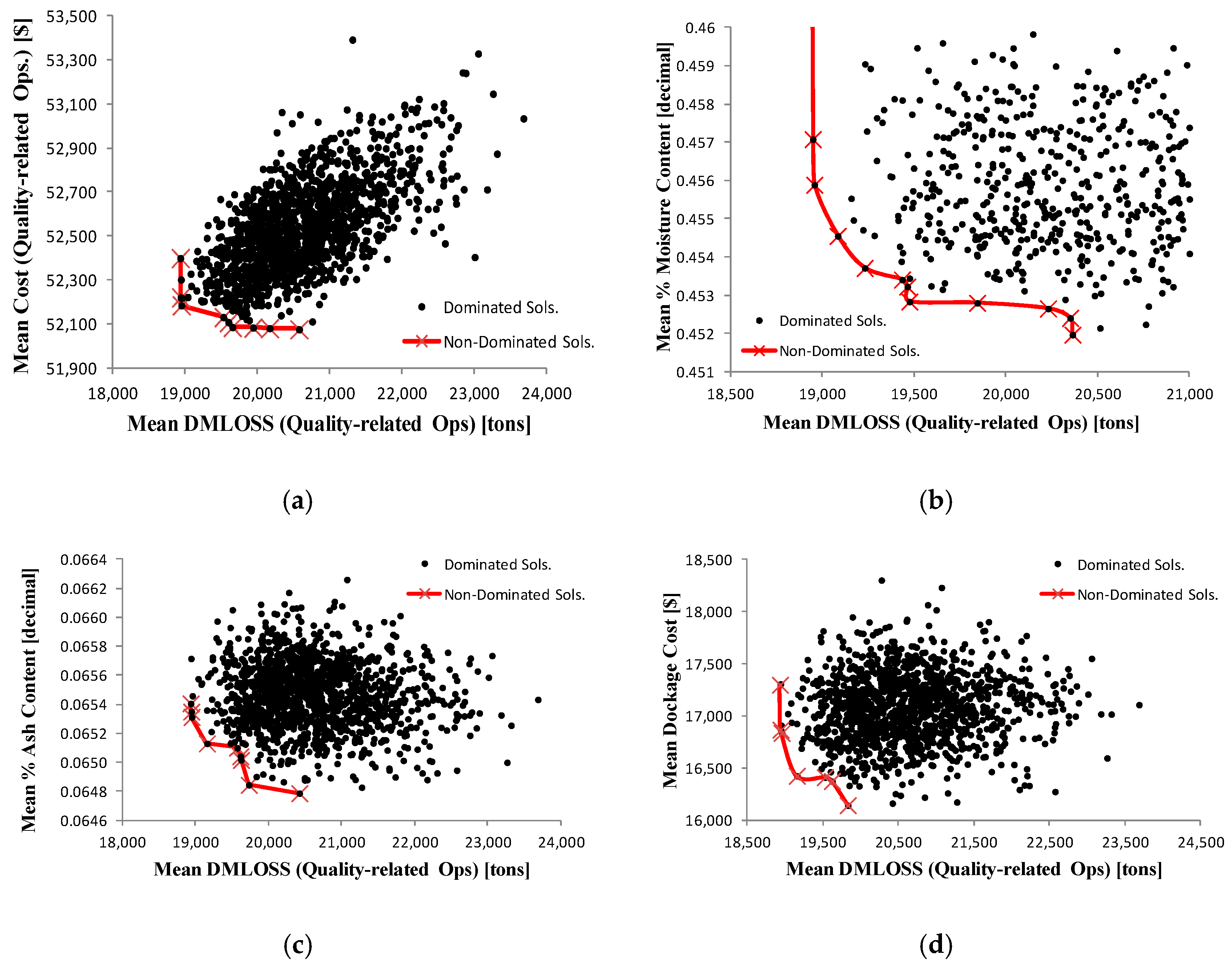

Figure 10.
Many-objective set of non-dominated solutions (schedule (*)).

Figure 11.
Hypervolume indicator approach (note: schedule 1 = schedule (*)).

Figure 12.
Solutions 1 and Solutions 682 (schedule 1).


Table 1.
Models for biomass SCs.
| Title | Author | Objective/Feedstock | Method | IBSAL |
|---|---|---|---|---|
| Biomass Supply Chains | ||||
| Development of a multicriteria assessment model for ranking biomass feedstock collection and transportation systems | Kumar et al. [9] | Rank alternatives for the collection and transportation of biomass. Feedstock: Biomass (corn stover). | Multicriteria assessment methodology (PROMETHEE I, II) and IBSAL | √ |
| Switchgrass (Panicum vigratum, L.) delivery to a biorefinery using integrated biomass supply analysis and logistics (IBSAL) model | Kumar and Sokhansanj [10] | Evaluate a collection systems of switchgrass and analysis of the related costs, energy input, and carbon emissions. Feedstock: Switchgrass | Discrete event simulation | √ |
| Cotton logistics as a model for a biomass transportation system | Ravula et al. [11] | Determine the operating parameters for reducing the transportation cost of biomass. Feedstock: Cotton gin (analogously to biomass). | Discrete event simulation | |
| The impact of agricultural residue yield range on the delivered cost to a biorefinery in the Peace River region of Alberta, Canada | Stephen et al. [12] | Evaluate the impact of residue yield on the biomass delivered cost. Feedstock: Straw and chaff from wheat, barley, and oats. | Discrete event simulation | √ |
| Techno-economic analysis of using corn stover to supply heat and power to a corn ethanol plant–Part 1: Cost of feedstock supply logistics | Sokhansanj et al. [13] | Propose a supply chain for corn stover to produce heat and power for a dry mill ethanol plant. Feedstock: Corn stover. | Discrete event simulation | √ |
| A mathematical model to design a lignocellulosic biofuel supply chain system with a case study based on a region in Central Texas | An et al. [14] | Maximize the profit of a lignocellulosic biofuel supply chain. Feedstock: Switchgrass. | Multi-commodity flow mathematical model | |
| Impact of distributed storage and pre-processing on Miscanthus production and provision systems | Shastri et al. [15] | Analyze the cost reduction from implementing distributed storage and pre-processing at satellite storage locations. Feedstock: Miscanthus. | Mixed integer linear programming (MILP) (BioFeed) optimization model | |
| Economic and energy evaluation of a logistics system based on biomass modules | An and Searcy [16] | Minimize the feedstock costs in a logistic system by maximizing highway load and minimizing load/unload times. Feedstock: Cotton (analogously to biomass) | Discrete event simulation | √ |
| An analysis of logistic costs to determine optimal size of a biofuel refinery | Larasati et al. [17] | Analyze the impact of logistic costs on the size of cellulosic ethanol biorefineries. Feedstock: Switchgrass. | Variable distance on grids approach | |
| Development of an integrated tactical and operational planning model for supply of feedstock to a commercial-scale bioethanol plant | Ebadian et al. [18] | Integrate the tactical and operational levels in the biomass supply chain for a commercial-scale cellulosic ethanol plant. Feedstock: Multi-biomass. | Discrete event simulation/Mixed-integer linear programming | |
| Biomass round bales infield aggregation logistics scenarios | Igathinathane, et al. [19] | Evaluate logistic scenarios for aggregating biomass bales to a field-edge stack or a storage. Feedstock: Biomass. | Computer simulation | |
| Evaluation of a modular system for low-cost transport and storage of herbaceous biomass | Searcy and Hartley [20] | Optimize the harvest of energy sorghum in the humid southern region by using a modified cotton module builder for the formation of modules. Feedstock: Energy sorghum. | Discrete event simulation | √ |
| Analyzing and comparing biomass feedstock supply systems in China: corn stover and sweet sorghum case studies | Ren et al. [21] | Analyze the harvest, collection, storage, transportation, preprocessing, handling, and queuing operations in the rural China biomass supply system. Feedstock: Corn stover and sweet sorghum. | System’s dynamics. Biomass Logistic Model (BLM) framework (BLM Sino-Feedstock Supply (FS)) | |
| Simulation-based multi-objective model for supply chains with disruptions in transportation | Chavez et al. [22] | Optimize the supply of agricultural products by using a simulation-based optimization model. Feedstock: Agricultural products. | Simulation-based Optimization | |
| Modelling a biomass supply chain through discrete-event simulation | Pinho et al. [23] | Providing a decisions tool for the biomass supply chain management services. Feedstock: Wood chip supply to a co-generation power plant. | Discrete event simulation (SIMEVENTS) | |
| Quantifying the impact of feedstock quality on the design of bioenergy supply chain networks | Castillo-Villar, Minor-Popocatl, and Webb [24] | Present a mixed-integer quadratically constrained programming model that minimizes the bioethanol SC, considering quality related costs. Feedstock: Logging residues. | Mixed-integer quadratic programming | |
| Development of the IBSAL model | ||||
| Development and implementation of integrated biomass supply analysis and logistics model (IBSAL) | Sokhansanj et al. [7] | Describe the development of the IBSAL model. Feedstock: Corn stover. | Discrete event simulation | √ |
| Development of the Integrated Biomass Supply Analysis and Logistics Model (IBSAL) | Sokhansanj, Turhollow, and Wilkerson [25] | Detailed description of the IBSAL model. Feedstock: Corn stover. | Discrete event simulation | √ |
| A new simulation model for multi-agricultural biomass logistics system in bioenergy production | Ebadian et al. [26] | Propose a model for the supply of a mixture of feedstock to a cellulosic ethanol plant. Feedstock: Multi-agricultural. | Discrete event simulation (IBSAL-MC (multi-crop)) | √ |
| Methods to optimise the design and management of biomass-for-bioenergy supply chains: A review | Meyer et al. [27] | Present an overview of the optimization methods and model focusing on the design of biomass SCs. Feedstock: Biomass. | Various methods | |
| The ExtendSim Optimizer | Diamond [28] | Describe the technique used by the ExtendSim Optimizer®™ to find the best set of parameters for a simulation model. Feedstock: N/A. | Simulation optimization | |
| Availability of feedstock and technologies | ||||
| Availability of corn stover as a sustainable feedstock for bioethanol production | Kadam and McMillan [29] | Analyze the potential long-term amount of corn stover available to ethanol plants. Feedstock: Corn stover. | Analysis of a generalized model for stover production and removal | |
| Large-scale production, harvest and logistics of switchgrass (Panicum virgatum L.)—Current technology and envisioning a mature technology | Sokhansanj et al. [30] | Evaluation of technologies for the production, harvest, storage, and transportation. Feedstock: Switchgrass. | Empirical | |
| Evaluation of a modular system for low-cost transport and storage of herbaceous biomass | Searcy and Hartley [20] | Optimize the harvest of energy sorghum in the humid southern region by using a modified cotton module builder for the formation of modules. Feedstock: Energy sorghum. | Discrete event simulation | √ |
| Influence of weather on the predicted moisture content of field chopped energysorghum and switchgrass | Popp et al. [31] | Determine the effect of weather on harvested moisture content. Feedstock: Switchgrass and energy sorghum. | Discrete event simulation | √ |
Table 2.
Equipment input data.
| Equipment | Input data |
|---|---|
| Mower-Conditioner | Width (ft), field speed average (mph), field efficiency (dec. fraction), machine efficiency, horsepower (hp), custom cost ($/h), annual fixed cost ($), variable cost ($/h), labor cost ($/h), purchase price ($), number of equipment, number of operators, machine biomass loss (decimal), and moisture content with zero machine loss (decimal w.b.) |
| Windrow-Tractor | Power, (hp), total cost ($/h), annual fixed cost ($), variable cost ($/h), labor cost ($/h), and purchase price. |
| Rectangular Baler | Baling pick up width (ft), field average speed (mph), field efficiency (dec. fraction), machine efficiency, power requirement (hp), custom cost ($/h), annual fixed cost ($), variable cost ($/h), labor cost ($/h), purchase price ($), number of equipment, number of operator, machine biomass loss (decimal), moisture content with zero machine loss (decimal w.b.), bale dimension width ( ft), bale dimension height (ft), bale dimension length (ft), bale density (lb/ft3), bales mass (ton), and cost of twine per bale ($/bale). |
| Tractor-Baler | Power (hp), total cost ($/h), annual fixed cost ($), variable cost ($/h), labor cost ($/h), and purchase price (S) |
| Infield-Transporter | Bale size 3x4x8 (volume ft3), bale density (lb/ft3), number of bale per load, load tie time—securing load (min/bale), load efficiency, travel speed full (mph), travel speed empty (mph), efficiency travel, unloading weight and inspection time (min/bale), efficiency unload, power (hp), custom cost ($/h), annual fixed cost ($), variable cost ($/h), labor cost ($/h), purchase price ($), number of equipment, number of operators, machine biomass loss (decimal), moisture content with zero machine loss (decimal w.b.), and winding factor. |
| Loader Storage | Number of bales per load, weight of each bale (ton), loading time per load (min), unloading time per load (min), efficiency, horsepower (hp), custom cost ($/h), annual fixed cost ($), operating cost ($/h), labor cost ($/h), purchase price ($), number of equipment, number of operators, machine biomass loss (decimal), and moisture content with zero machine loss (decimal w.b.) |
| Flatbed Trailer | Bale size 3x4x8 (volume ft3), bale density (lb/ft3), number of bale per load, load tie time—securing load (min/bale), load efficiency, travel speed full (mph), travel speed empty (mph), efficiency travel, unloading weight and inspection time (min/bale), efficiency unload, power (hp), custom cost ($/h), annual fixed cost ($), variable cost ($/h), labor cost ($/h), purchase price ($), number of equipment, number of operators, machine biomass loss (decimal), moisture content with zero machine loss (decimal w.b.), and winding factor. |
| Truck-Tractor | Power (hp), total cost ($/h), annual fixed cost ($), variable cost ($/h), labor cost ($/h), and purchase price |
| Bale Wrapper | Purchase price, stone pad cost ($/m2), cost of plastic wrap per bale, wrapping time (min/bale) |
| Tarp | Tarp cost ($/ft2), labor cost to remove and place tarps ($/ft2), and tarp useful life (years) |
Table 3.
SA schedules.
| Sched. | Pr | MinTemp (all) | MinOFVal (all) | Rejectsmax | Runsmax | Acceptsmax | k | Ali | NBi |
|---|---|---|---|---|---|---|---|---|---|
| * | 0.95 | 0.001 | 0.01 | 10 | 10 | 10 | 1 | 10 | 100 |
| ** | 0.6 | 0.001 | 0.01 | 5 | 5 | 5 | 1 | 10 | 10 |
| *** | 0.6 | 0.001 | 0.01 | 10 | 10 | 10 | 1 | 10 | 100 |
© 2017 by the authors. Licensee MDPI, Basel, Switzerland. This article is an open access article distributed under the terms and conditions of the Creative Commons Attribution (CC BY) license (http://creativecommons.org/licenses/by/4.0/).
Share and Cite
MDPI and ACS Style
Chavez, H.; Castillo-Villar, K.K.; Webb, E. Development of the IBSAL-SimMOpt Method for the Optimization of Quality in a Corn Stover Supply Chain. Energies 2017, 10, 1137. https://doi.org/10.3390/en10081137
AMA Style
Chavez H, Castillo-Villar KK, Webb E. Development of the IBSAL-SimMOpt Method for the Optimization of Quality in a Corn Stover Supply Chain. Energies. 2017; 10(8):1137. https://doi.org/10.3390/en10081137
Chicago/Turabian StyleChavez, Hernan, Krystel K. Castillo-Villar, and Erin Webb. 2017. "Development of the IBSAL-SimMOpt Method for the Optimization of Quality in a Corn Stover Supply Chain" Energies 10, no. 8: 1137. https://doi.org/10.3390/en10081137
Note that from the first issue of 2016, this journal uses article numbers instead of page numbers. See further details here.