Numerical Investigation of the Effect of Variable Baffle Spacing on the Thermal Performance of a Shell and Tube Heat Exchanger

1
Faculty of Engineering, Department of Automotive Engineering, Uludağ University, Görükle, Bursa 16059, Turkey
2
Faculty of Technology, Department of Automotive Engineering, Amasya University, Amasya 05100, Turkey
*
Author to whom correspondence should be addressed.
Energies 2017, 10(8), 1156; https://doi.org/10.3390/en10081156
Submission received: 23 June 2017
/
Revised: 27 July 2017
/
Accepted: 1 August 2017
/
Published: 7 August 2017
Abstract
:In this present study, numerical and theoretical analysis were both used to investigate the effect of the variable baffle spacing on the thermal characteristics of a small shell and tube heat exchanger. The numerical study was performed by using a three dimensional computational fluid dynamics (CFD) method and the computations were performed under steady-state conditions. We employed five different cases where the first had equal baffle spacing and the others had variable ones considering different configurations for balancing the pressure drop on the shell side. Theoretical calculations were run using the Bell-Delaware and Kern methods which are the most commonly used methods in the available literature. We show that the thermal performance of a shell and tube heat exchanger can be improved by evaluating together the results of the CFD and Bell-Delaware methods. From the numerical results, we can say that variable spacing with centered baffle spacing scheme can be proposed as an alternative shell side construction layout compared to an equal baffle spacing scheme. The numerical results were in good agreement with the theoretical data in the available literature.
1. Introduction
Heat exchangers are devices made for efficient heat transfer from one zone to another in order to transfer energy and they are widely used in different industries like the automotive, heating, ventilation and air conditioning (HVAC), chemical and food industry and so on [1,2]. The shell and tube heat exchanger is an indirect contact type heat exchanger and there are considerable reasons to prefer the shell and tube heat exchanger, such as relatively simple manufacturing, multi-purpose applicability, robust geometry construction, easy maintenance, etc. Certain standards and correlations proposed by the Tubular Exchanger Manufacturers Association (TEMA) have to be considered when a well-designed shell and tube heat exchanger is desired for industrial applications. In the shell and tube heat exchanger there are two main fluid flows, one fluid flow that goes through the tubes while the other flows on the shell side [3,4,5]. In a baffled shell and tube heat exchanger, the baffles are used for different reasons such as providing support for tubes, obtaining a desirable fluid velocity to be maintained for the shell-side fluid flow, and preventing the tubes from vibrating. They also direct the shell side flow to enhance the heat transfer coefficient but their usage conversely produces an increased pressure drop [6]. Therefore, their dimensions and locations have to be optimized or they have to be replaced with the other types which have better heat transfer efficiency and lower pressure drops [7,8,9,10]. There are numerous studies on the impact of the baffle cut, number of baffles, baffle type, etc. on the thermal performance of the shell and tube heat exchanger in the available literature, however there is a limited amount of research on the effect of variable baffle spacing schemes on the heat transfer rate and pressure drop of a small shell and tube heat exchanger. Baffle spacing is one of the most important parameters used in the design of shell and tube heat exchangers. Closer spacing causes a higher heat transfer rate and pressure drop. On the other hand, a higher baffle spacing reduces both the heat transfer rate and pressure drop [11]. In this study, we investigated the impact of variable baffle spacing on the thermal characteristics of a shell and tube heat exchanger. As the default shell and tube heat exchanger an E shell type was selected which is the most commonly used due to its low cost and simplicity. The shell and tube heat exchanger used in this study had one shell and one pass with 19 tubes and seven baffles. In theoretical calculations for predicting the overall heat transfer coefficient, the convective heat transfer coefficients for the shell and tube sides are needed. On the tube side, well known correlations have to be selected according to the flow conditions. On the other hand, the shell side analysis is more complex than the tube side one because of several additional parameters that affect the shell side flow. On the shell side of the heat exchanger, the Kern and Bell-Delaware methods are the common methods used in the literature to calculate the heat transfer coefficient and pressure drop. Comparing these two methods, the Kern method is also only suitable for preliminary sizing whereas the Bell-Delaware method is a very detailed method that takes into account the effects of various leakage and bypass streams on the shell side. The Bell-Delaware method gives also the most reliable results for the shell side analysis [1,12,13]. However, while all these theoretical calculations indicate the deficiencies of shell side design in general these methods do not give any information about the location of these weaknesses. On the other hand, a well designed and built computational fluid dynamics (CFD) numerical model can be a useful tool to obtain the flow and heat transfer characteristics of a shell and tube heat exchanger. The CFD method with these common correlations can be utilized to get the appropriate flow and heat transfer characteristics taking into account the desired heat transfer rate and pressure drop. The CFD method can be used both in the rating and iteratively in the sizing of heat exchangers [14]. On the other hand, to get a successful CFD simulation for a detailed heat exchanger model, in the numerical computations, we chose a small shell and tube heat exchanger to evaluate the effect of variable baffle spacing on the heat transfer coefficient and also pressure drop that can be compared with the correlation-based ones.
2. Materials and Methods
2.1. Theoretical Study
The total heat transfer rate between two different fluid streams can be easily calculated by using Equations (1) and (2) under steady-state conditions assuming negligible heat transfer between the heat exchanger and its surroundings:
On the other hand the temperature difference in the heat exchanger varies with the location in both shell and tube sides. Thus, for the design process, the total heat transfer rate can be written by using logarithmic mean temperature difference (LMTD) shown in Equation (3):
where Uf is the overall heat transfer coefficient described in Equation (5) considering fouling resistance, A is the total heat transfer area of a heat exchanger and the ΔTlm can be calculated as a function of inlet and outlet temperatures both of hot and cold fluids by using Equation (4):
In this study, the fouling resistance is assumed negligible in theoretical calculations, thus Equation (5) can be rewritten for cylindrical geometries and the final form of the overall heat transfer coefficient based on the outer diameter of the tube which is used in this study is described in Equation (6) for clean surfaces. The use of Equation (6) requires the convective heat transfer coefficients for shell and tube sides. In this study, the shell side heat transfer coefficient and pressure drop for various baffle spacings were calculated by using the Kern and Bell-Delaware methods described below. The heat transfer coefficient of the tube side was calculated by using the appropriate correlation known as the Petukhov-Kirillov method and the flow was assumed as turbulent (Equations (7)–(10)):
2.1.1. Shell Side Heat Transfer Coefficient and Pressure Drop Using the Kern Method
In the Kern method, all results are based on a constant baffle cut (Bc) ratio which is taken as 25% in this study. The shell side heat transfer coefficient can be calculated with the correlation suggested by Mc Adams and expressed by Equation (11), where ho is the shell-side heat transfer coefficient, De is the equivalent diameter on the shell side and is calculated by using Equation (12) and Gs is the shell side mass velocity which is the ratio of mass flow rate to the bundle crossflow area at the center of the shell that can be calculated from Equation (13) [15]. The bundle crossflow area can be calculated using shell side inner diameter (Ds), clearance between adjacent tubes (C), the distance between two successive baffles (B) and the pitch size (Pt) (Equation (14)):
In this method, the pressure drop for the shell side can be calculated with Equation (15), where Nb is the number of baffles, is calculated from Equation (16) where μ is the dynamic viscosity and the friction factor (f) for the shell side can be calculated from Equation (17) considering the range of the Reynolds number described:
2.1.2. Shell Side Heat Transfer Coefficient and Pressure Drop Using the Bell-Delaware Method
The Bell-Delaware method is more complicated than the Kern method because of some additional parameters that are involved in the calculations. These parameters concern various leakages and bypass streams on the shell side and their effect on the shell side ideal heat transfer coefficient is described by Equation (18): The ideal heat transfer coefficient (hid) described in the Bell-Delaware method for pure crossflow in an ideal tube bank and is calculated from Equation (19), where Ji is Colburn j-factor and it can be found as a function of the shell side Reynolds number, As is the cross-flow area at the centerline of the shell for one cross-flow between two baffles. Jc is the correction factor for baffle cut and spacing, Jl is the correlation factor for baffle leakage effects including tube-to-baffle and shell-to-baffle leakage, Jb is the correction factor for bundle bypassing effects and Js is the correction factor for variable baffle spacing at the inlet and outlet. Jr is only appropriate if Re is less than 100. This factor can be selected as 1.00 if Re > 100. Baffle leakage effects were not considered in the CFD model so the Jl factor was assumed as 1. Js is a correction factor if the baffle spacing length is different in the inlet and outlet fluid zones. In this study, the value of this length was equal to each other for these zones, thus the Js factor was assumed as 1. The details of this method can be found in [1]:
For shell side Reynolds number we used Equation (20) where do is the outer diameter of a one tube and As is the crossflow bundle area described in Equation (14). The Reynolds number is computed to be about 2773, thus the shell side flow is assumed as turbulent:
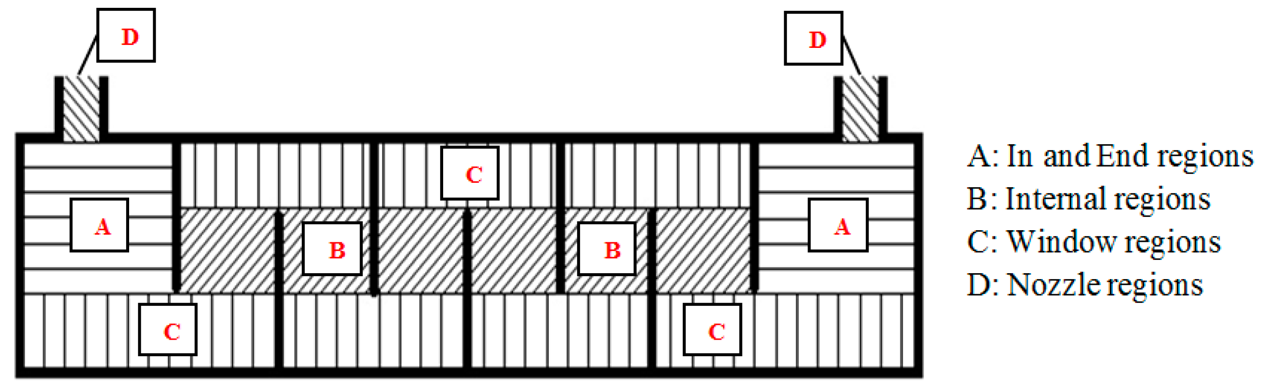
In this method the total pressure drop for the shell side (Δps) is calculated considering entering and leaving (Δpe), internal cross-flow (Δpc) baffle window (Δpw) and the nozzle (Δpn) regions, the detailed information about these calculations can be found in references [16] and [17] (Equation (21)). These pressure drop regions are shown in Figure 1 for shell and tube heat exchangers in general:
2.2. Numerical Study
2.2.1. CAD Model of the Heat Exchanger
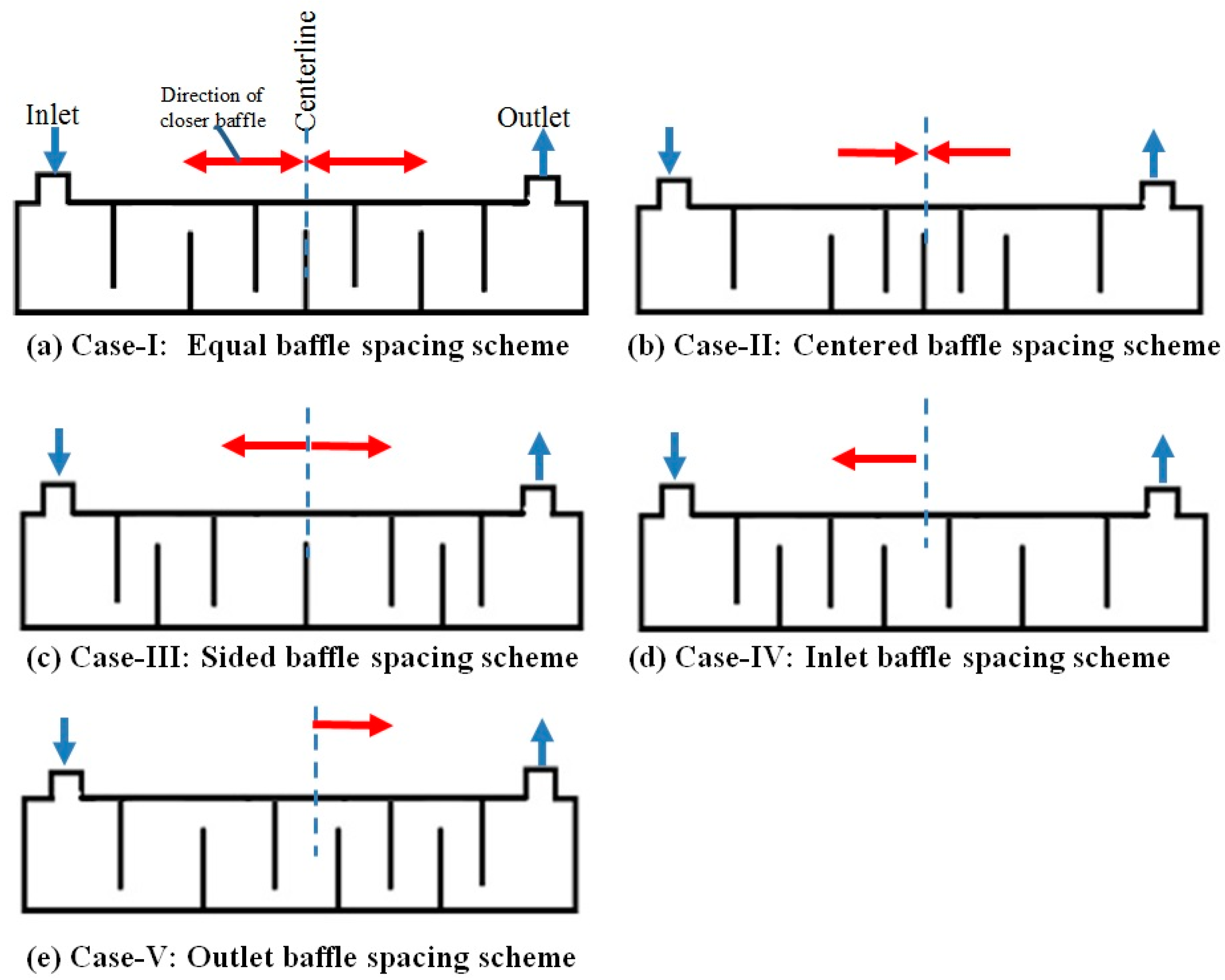
We considered three different locations that can be taken as a reference point for the comparison of the thermal performance. These locations were selected at inlet, outlet and the center of the heat exchanger. This can be also examined in different configurations but five different baffle spacing schemes were selected for the numerical simulations to evaluate the effect of variable baffle spacing on the heat transfer characteristics in terms of using these reference locations.
In the first case the heat exchanger had equal baffle spacing length and the other cases it had a variable one. On the other hand, in the second case, the baffle spacing length decreases when approaching the center line of the heat exchanger. The third case had an opposite structure to the second case. For the fourth and fifth cases, a baffle spacing length which decreases from centerline to the inlet and outlet zones, respectively, was selected. These variable baffle spacing schemes and the dimensions are shown in Figure 2 and Figure 3 and Table 1. We selected these five different schemes for the comparison of the numerical results in view of pressure drops and heat transfer rates.
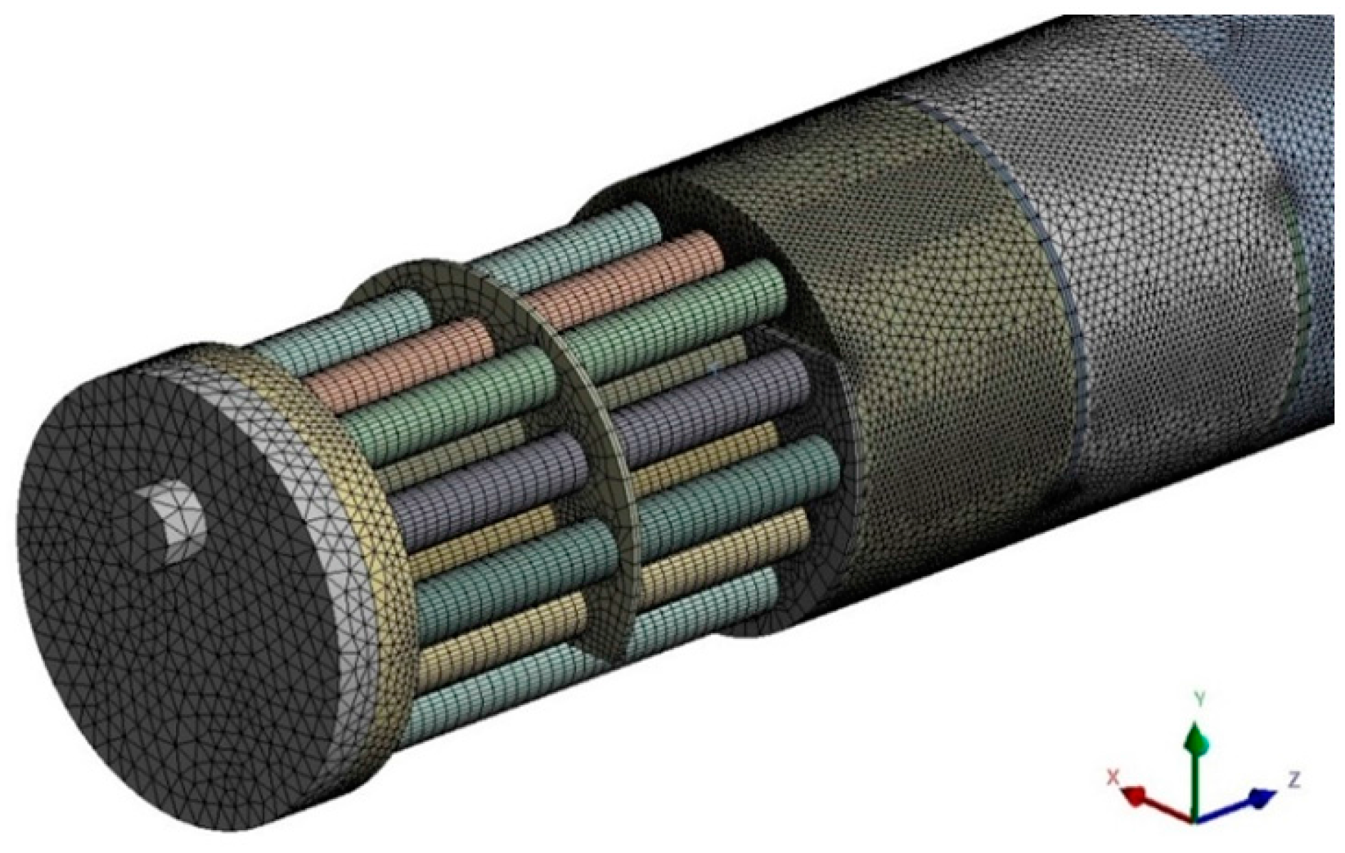
2.2.2. Mesh Structure and Boundary Conditions of Numerical Calculations for Shell and Tube Heat Exchanger
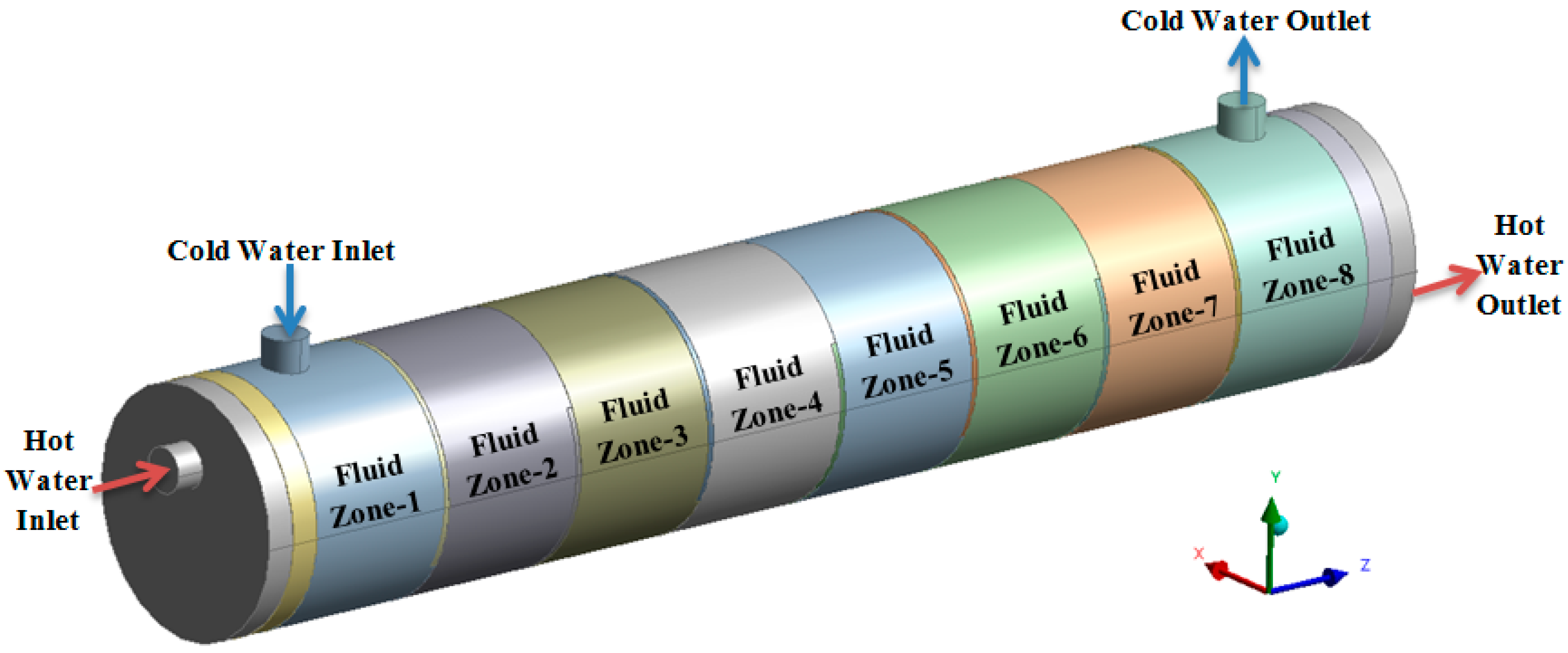
In the numerical calculations of all cases, the computational domain had eight fluid zones in the shell side for getting comparative numerical detailed results (Figure 5). The multi-zone approach was used to model the heat exchanger and all these zones had tetrahedral mesh elements due to the complexity of the CAD model. The number of total elements was about 6.0 million and the mesh should be well designed to resolve the important flow features which are dependent upon flow condition parameters.
In numerical calculations, mesh generation is very crucial for getting accurate predicted results and reducing the computation time [9,12,14,18,19]. The mesh structure of the surfaces of the computational domain and the section view of this domain are shown in Figure 6. Today, there are many computer software packages for flow field and heat transfer analysis. For the mesh generation and the numerical solution, the Ansys Fluent package software program was used. In this software flow and temperature fields were computed by a three dimensional CFD method. This software solves continuum, energy and transport equations numerically and the coupled algorithm was chosen for pressure-velocity coupling, the k-ε realizable model was used for turbulence modeling and this model was used for such calculations due to stability and precision of the numerical results in the available literature [6,12,18,19,20,21,22]. The governing equations for steady state conditions are shown below:
In Equation (22), Φ is the dissipation function that can be calculated from:
All numerical calculations were performed under steady state conditions and in the numerical calculations, water was selected as both the shell and tube side fluid in the numerical model of the heat exchanger. The mass flow rates of the hot and cold water were set to 0.3 kg/s and 0.2 kg/s and the temperature values of these zones were set to 50 °C and 10 °C, respectively. The detailed solver settings and the boundary conditions used in this numerical study are shown in Table 3.
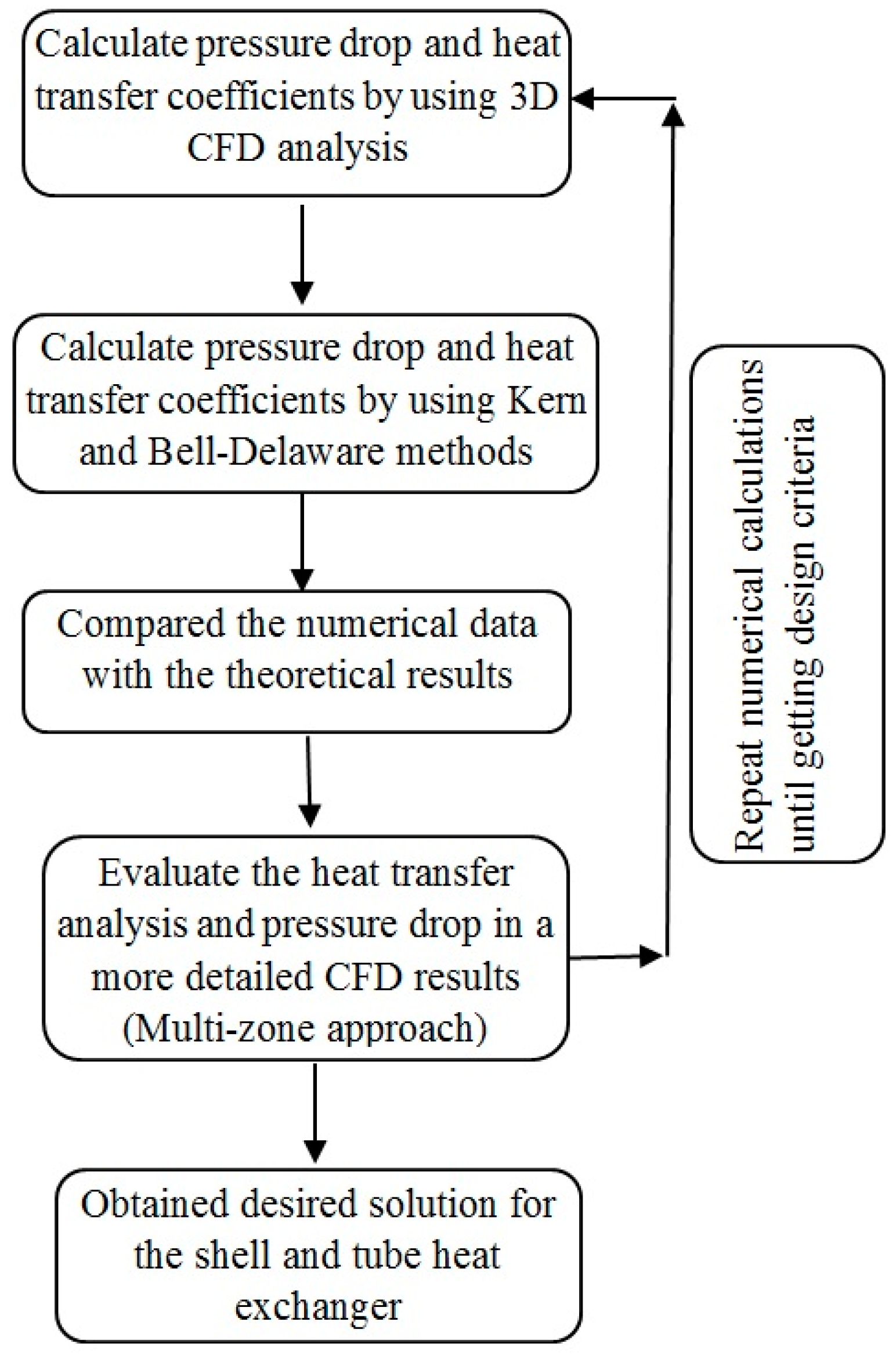
The flow chart of the numerical simulation used in this study is shown in Figure 7. In the first stage, 3D CFD analysis of a shell and tube heat exchanger was achieved by using a commercial CFD solver. When the entire fluid domain is modeled as a single continuum zone, the numerical data can be obtained only for this zone and getting the computed values of temperature, velocity and pressure between baffles becomes difficult. We used a multi-zone approach in which the entire fluid domain for CFD analysis was divided into sub-zones as shown in Figure 5 and Figure 6. These sub-zones can helpful to get the numerical solution data between two successive fluid zones compared to the single zone. These sub-zones were used to obtain the thermal characteristics and pressure drop in an efficient way. In this content, we can easily say that multi-zone solution scheme including solid and fluid zones can be used to evaluate the heat transfer characteristics and pressure drop in a more detailed way compared to the single zone approach because the multi-zone approach enables one to investigate each fluid zone individually in view of the heat transfer coefficient, pressure drop, temperature and velocity distributions. On the other hand, this approach can be used to evaluate the results such as the weaknesses (different leakage flow paths, bypass streams for different flow zones, temperature and velocity distribution for each zone etc.) on the shell side for different operating conditions. Moreover, using a 3D CFD model, the effect of the main important parameters such as baffle spacing length and baffle cut on the heat transfer and pressure drop in shell side can be obtained easily in this stage.
The validation of the numerical results can be achieved by comparison with the theoretical results of common methods like the Kern and Bell-Delaware methods. Thus multi-zone CFD approach used together with common theoretical methods can be useful for getting better design solution considering the maximum pressure drop limit and desired heat transfer rate of the heat exchanger. The desired configuration based on the numerically obtained temperature and flow fields can be achieved iteratively and this numerical solution procedure is shown in Figure 7.
In the numerical calculations, the 3D model of the heat exchanger was obtained considering inlet and outlet plenums, whereas in the literature, some numerical investigations were performed by applying a constant mass flow rate for each tube individually and constant temperature boundary conditions were applied to the tube surfaces in general, but in this study, we also considered the effect of the velocity distribution of the inlet and outlet regions (plenum) on the flow inside the tubes and the shell and tube side flows were both solved simultaneously with energy equations [5,12]. On the other hand, we also employed solid zones such as tube walls, shell body, baffles and inlet and outlet nozzles etc. to include conjugate heat transfer in this numerical study.
3. Results and Discussion
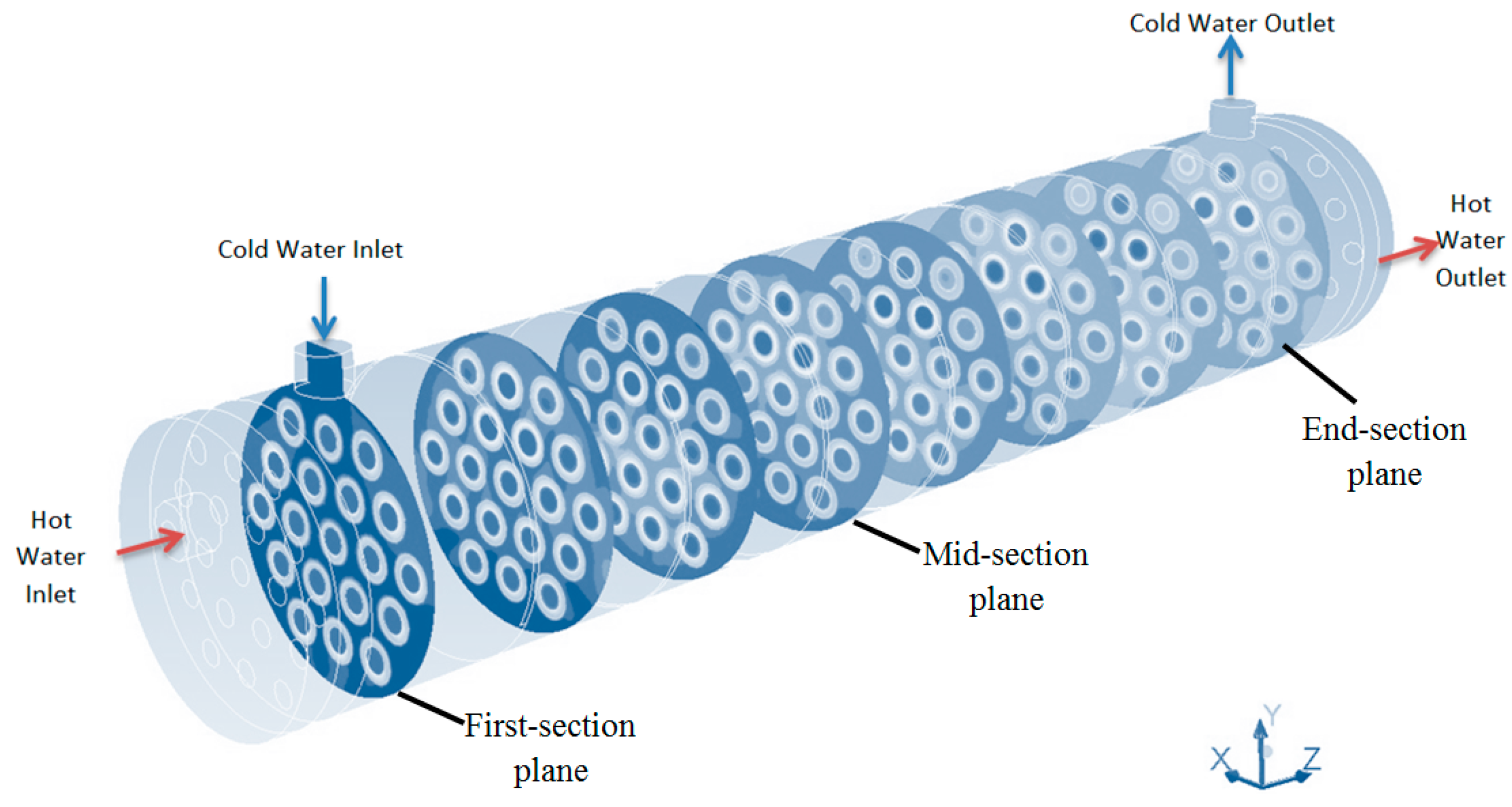
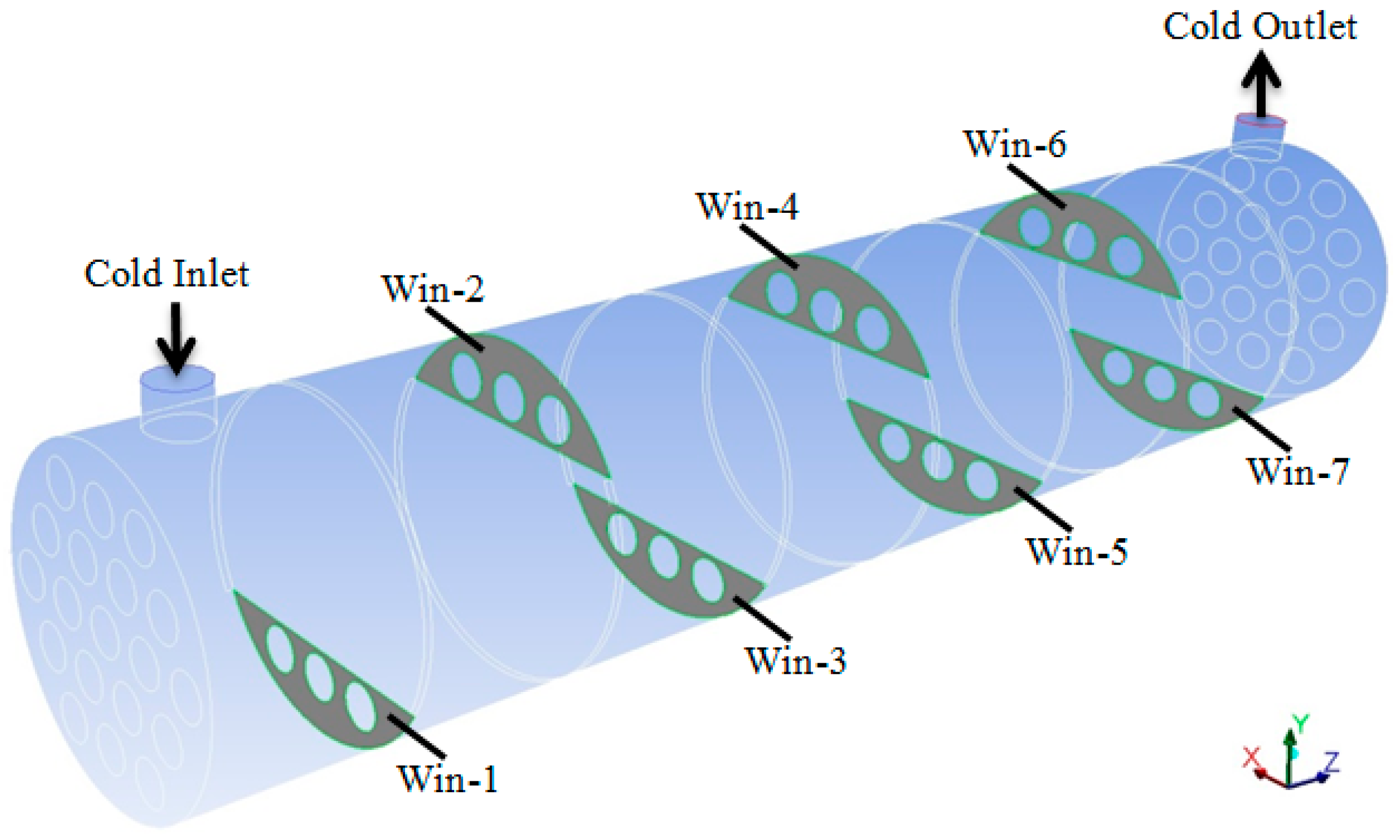
For getting the comparative numerical results, we defined eight section planes in different zones (Figure 8). The first and end section planes are located at the mid-center of the nozzles and the other ones are located at the middle center of the each fluid zone. To evaluate the numerical data in terms of multi-zone approach, the each fluid zone had inlet and outlet faces, separately. These faces (window, inlet and outlet faces) are shown in Figure 9.
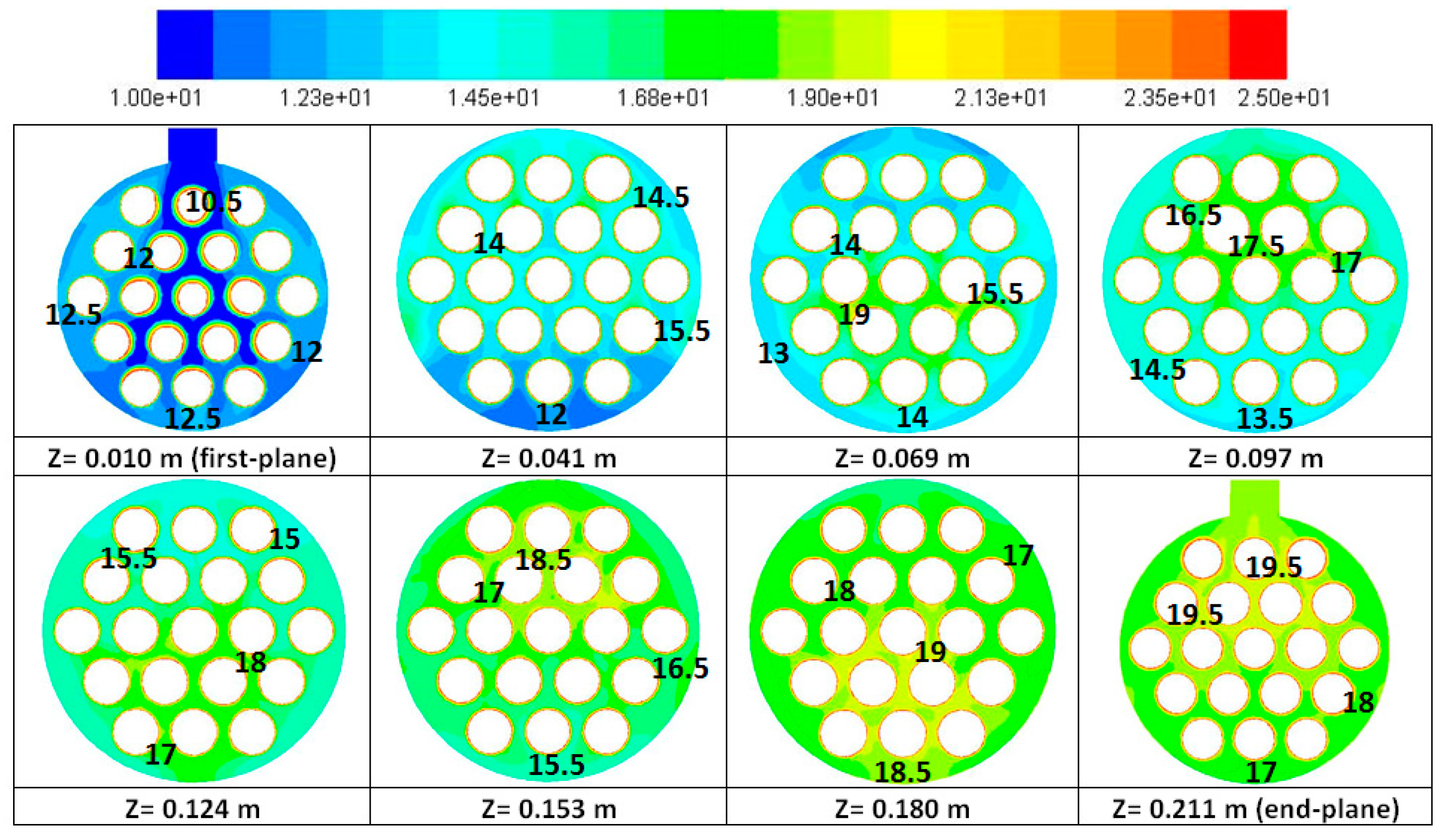
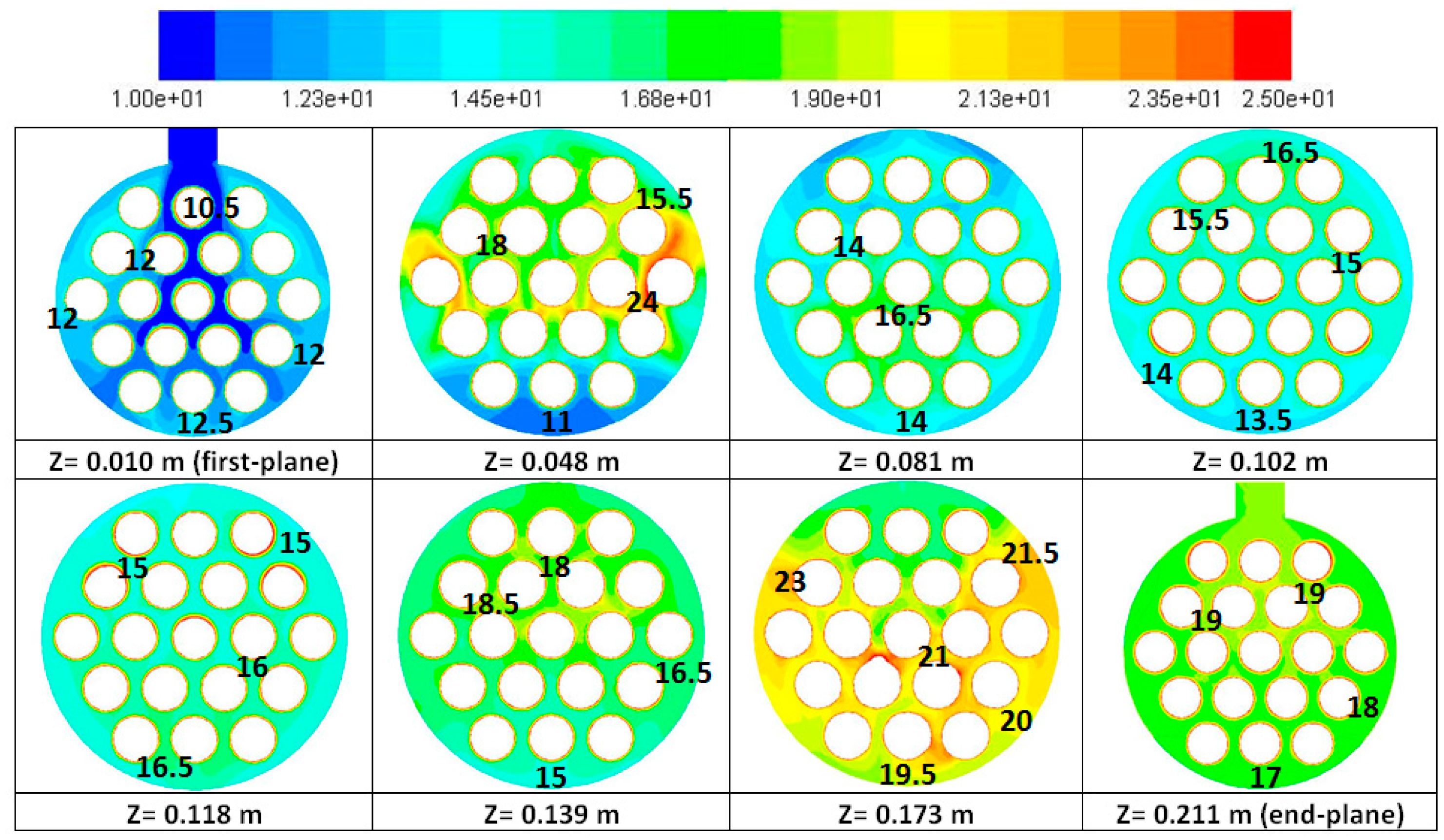
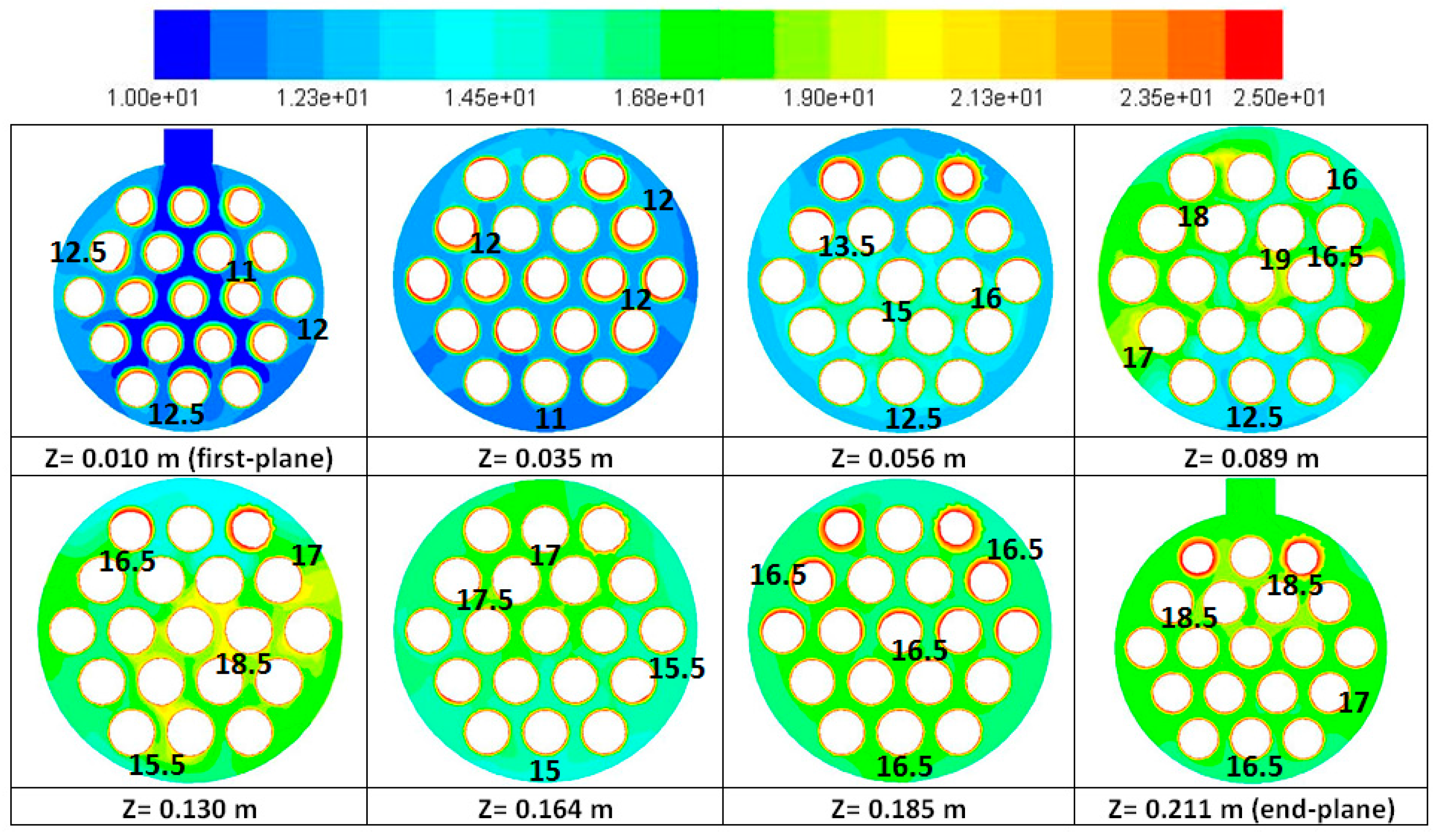
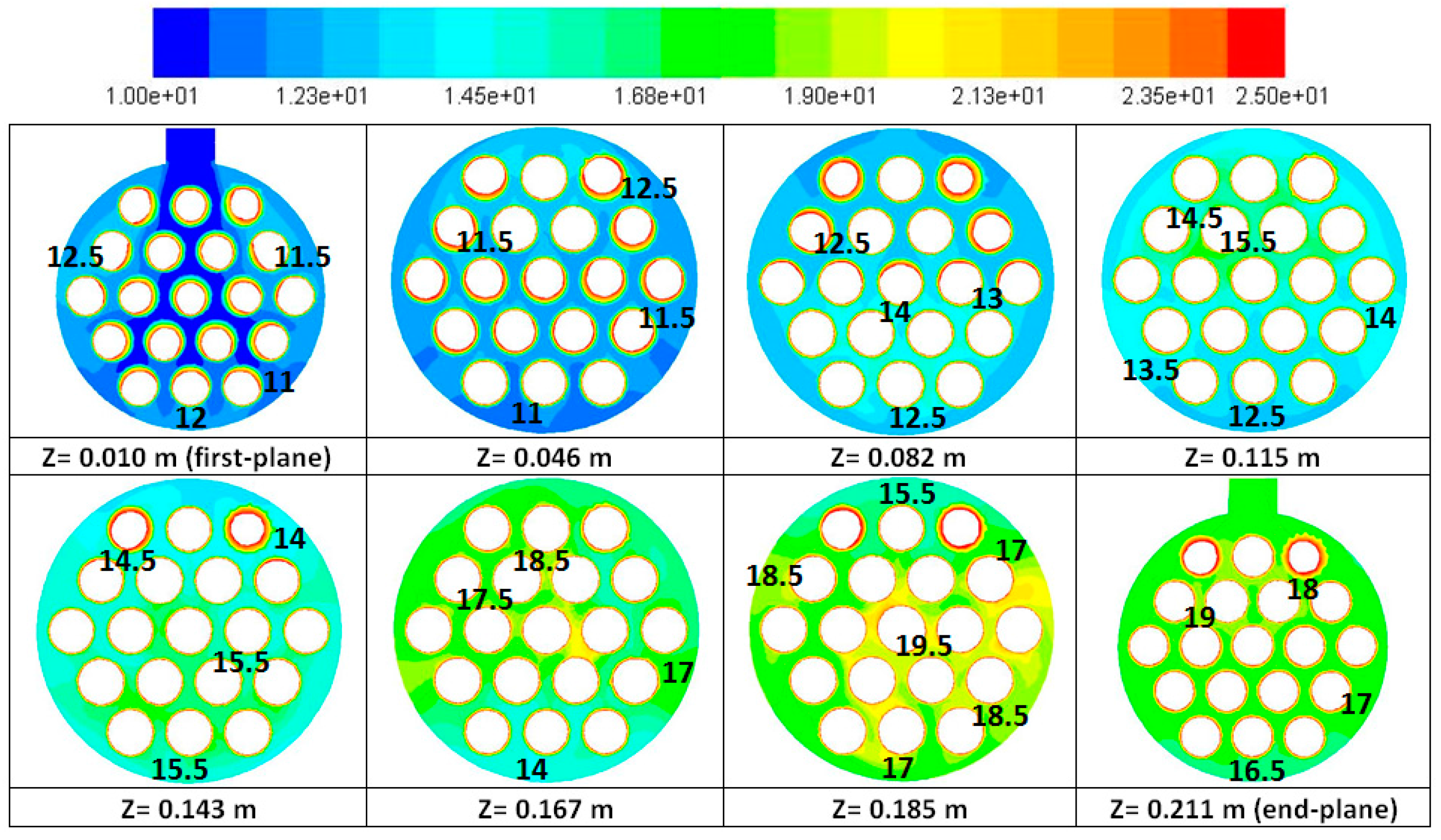
The predicted temperature values at these section planes are shown in Figure 10, Figure 11, Figure 12, Figure 13 and Figure 14. The calculated maximum temperature difference was about 2.5 °C in the first section plane for all cases. On the other hand, the predicted temperature values increased with the z-coordinate and the maximum values were computed at the location which had dense baffle spacing construction because this structure leads to an increase in the predicted temperature values in these section planes. Thus we can say that heat transfer rate strictly depends on the baffle spacing length.
From the calculated temperature values at the middle center of the each fluid zone the temperature values were lower than the others for the region aligned with the window area for all cases in general (Figure 10, Figure 11, Figure 12, Figure 13 and Figure 14). The maximum temperature difference between the first and end section planes were computed at about 9 °C for Case-I and Case-II. In these section planes, the calculated maximum temperature value was obtained for Case-II and it was computed about 23 °C at z = 0.173 m section plane which is located close to the middle plane of the heat exchanger. As a result of these numerical data, we can easily say that different baffle spacing scheme has a great effect on the temperature distribution of shell side and also the heat transfer rate. These results can be used for getting better designs in terms of heat transfer characteristics.
These computed numerical data for each zone is shown in Table 4 and Table 5. From the obtained results, the calculated pressure drop changed between 893 Pa and 1210 Pa for each zone. Due to the assignation of zero gauge pressure for the outlet surface to obtain the relative pressure drop between inlet and outlet sections, the maximum pressure drop was calculated from win-7 to the cold outlet surfaces. One of the reasons for this situation is that, the contraction at the outlet nozzle leads to a higher pressure drop. The maximum pressure drop that occurred in a single fluid zone was calculated at about 1600 Pa for Case-II. However, in this case, this leads to an increase in temperature values and also the heat transfer rate compared to the Case-III, Case-IV and Case-V. On the other hand the temperature difference between the cold inlet and outlet surfaces was predicted at about 7.2 °C for Case-III, Case-IV and Case-V. This value was computed as 8.1 °C and 8.0 °C for Case-I and Case-II, respectively. Thus, Case-I and Case-II have similar thermal properties in view of heat transfer rate and the pressure drop was calculated to be nearly equal, but the pressure drop should be adopted considering the best design configuration by changing baffle spacing length for Case-II.
The predicted heat transfer rates for each zone and total heat transfer rate for all cases are shown in Table 6. From the obtained numerical results, the calculated total heat transfer rates for Case-I and Case-II were about equal to 6.5 kW and these cases had similar properties in terms of thermal performance. The ratio of the total heat transfer rate to the computed heat transfer rate for Case-I was defined as a dimensionless number (Rh) and this value was computed as 0.98. These results shown that Case-II which had variable spacing with centered baffle spacing scheme had similar thermal properties compared to Case-I but more experimental investigation about this scheme has to be performed considering practical problems. The predicted total heat transfer rates for Case-III, Case-IV and Case-V were about 5.9 kW, thus these baffle spacing schemes had lower thermal performance than the others. The minimum predicted heat transfer rate was obtained for Case-III and Case-V.
The computed overall heat transfer coefficients, the total heat transfer rates and pressure drops for all cases are shown in Table 7. For the pressure drop calculations, we only used the Bell-Delaware method because the Kern method is just suitable for initial sizing problems but the Bell-Delaware method estimates shell side heat transfer coefficients and pressure drops more precisely. The baffle cut ratio was selected as 25% which is the reference value of the Kern method. From the results given in Table 7, the computed overall heat transfer coefficient by using the Kern and CFD methods were calculated to be 2533 W·m−2 K−1 and 2347 W·m−2 K−1, respectively, but this computed value was about 2270 W·m−2 K−1 from the Bell-Delaware method. In the CFD method, the effects of various leakage and bypass streams on the shell side were ignored, thus the computed value was higher than that one obtained from the Bell-Delaware method. The outlet temperature of the shell side, pressure drop and overall heat transfer coefficient were directly computed from the CFD results and the difference between the heat transfer rates for the shell and tube sides was nearly about 0.5 Watt, thus we can easily say that steady-state conditions were achieved for the CFD results. The calculated total pressure drop for Case-I was about 21 kPa and 18 kPa by using the CFD and Bell-Delaware methods, respectively.
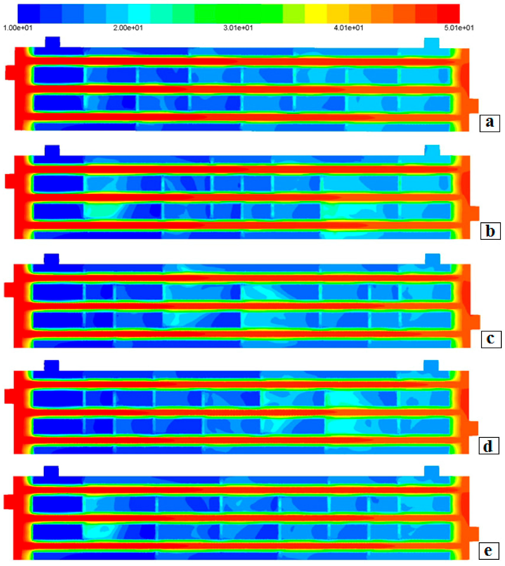
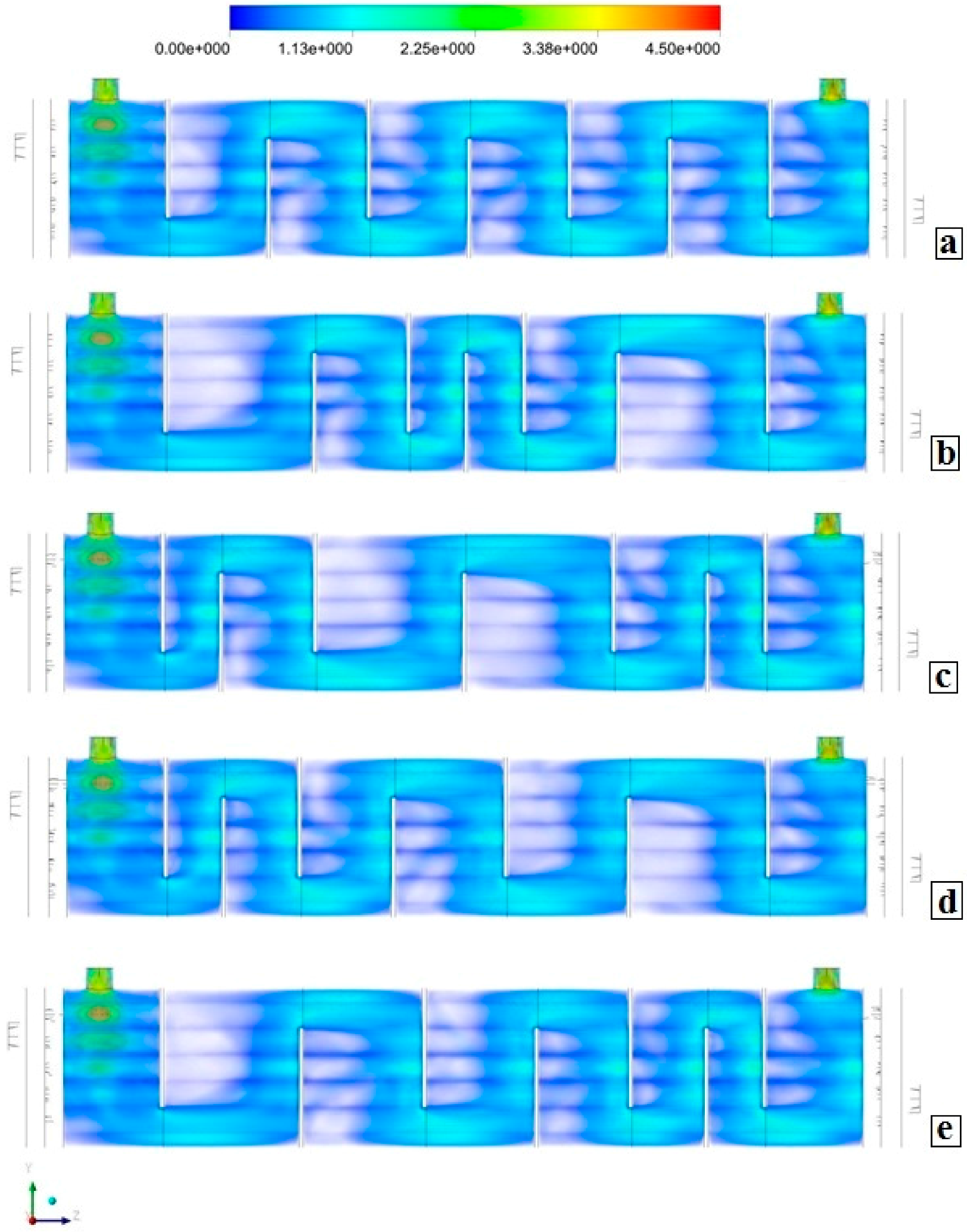
We also defined a horizontal plane parallel to flow direction in the middle center of the shell and tube heat exchanger and the calculated temperature distributions throughout the flow direction for all cases are shown in Figure 15. These results may be used to evaluate the heat transfer characteristics between the cold and hot fluid streams. As expected, the maximum temperature difference between the tube outer wall and the shell side fluid were predicted in the first fluid zone for all cases. This value decreased along the tubes and the minimum value was computed for the end zone. The higher temperature values were predicted in the second half of the heat exchanger and we can easily say that the baffle spacing length and scheme directly affected the temperature distribution in the center plane of the heat exchanger. The predicted velocity distribution in all fluid zones is shown in Figure 16 for all cases. The computed velocity value was obtained between 1.1 m·s−1 and 2.25 m·s−1 in general but the maximum value was computed about 4.5 m·s−1 near the nozzle regions due to contraction in the inlet and outlet regions. The calculated mass average velocity values for all fluid zones are shown in Table 8. The predicted mass average velocity values varied between 0.4 m·s−1 and 2.25 m·s−1 in general, however the maximum calculated value was 0.662 m·s−1 in fluid-zone 5 for Case-II due to effect of the dense baffle spacing scheme for that zone. The computed mass average velocity value in the first and end fluid zones was calculated at about 0.6 m·s−1 and 0.5 m·s−1, respectively, for all cases. It can be observed that a decrease in baffle spacing length leads to higher velocity values and the heat transfer rate will be higher with increasing velocity values.
4. Conclusions
In this study, numerical and theoretical analysis were both used to investigate the effect of variable baffle spacing on the thermal characteristics of a small shell and tube heat exchanger. As a result of these numerical computations, we can say that correlation-based approaches indicate the deficiencies of a shell and tube heat exchanger but the location of these weaknesses is not used in any of these methods. By using a well designed and built multi-zone CFD model, the flow and heat transfer characteristics of a shell and tube heat exchanger can be changed and improved. Another important result is that the Case-I which had equal baffle spacing configuration had the smallest pressure drop and highest thermal performance among all the schemes. On the other hand, the predicted temperature difference between the cold inlet and outlet surfaces was about 8 °C for Case-I and Case-II. Thus, we conclude that thermal performance of Case-II was close to that of Case-I but using the variable baffle spacing scheme in practical applications may cause difficulties such as manufacturing and maintenance problems, etc. More experimental investigations about this scheme have to be performed considering industrial applications. However, using a centered baffle spacing scheme leads to an increase in pressure drop and also the heat transfer rates, so design parameters have to be determined for the best configuration considering the maximum pressure drop limit and desired heat transfer rate of the heat exchanger. We can easily say that different baffle spacing schemes have a great effect on the temperature distribution of the shell side and also the heat transfer rate. These results can be used for getting the best design in terms of heat transfer characteristics of a shell and tube heat exchanger. Moreover, using the CFD model together with the correlation-based approaches not only indicates the weaknesses, but also predicts the location of the maximum pressure drop, variation of heat transfer rate and flow field and the effects of different baffle spacing schemes on the heat transfer characteristics of the shell and tube heat exchanger in a more detailed way. In this numerical study, the simulation results are compared with the results from the Kern and Bell–Delaware methods and the numerical results were in good agreement with the theoretical data, although in this study, the numerical data from the CFD solution were more compatible with the theoretical results calculated with the Kern method. However, more complicated parameters such as by-pass and leakage streams and various factors existing in the Bell-Delaware method leads to underestimated thermal performance results. We plan to investigate the transient thermal performance of a shell and tube heat exchanger in future studies considering different baffle spacing schemes and the other design configurations.
Author Contributions
Halil Bayram and Gökhan Sevilgen prepared this article Gökhan Sevilgen analysed the research data to contribute the design configurations and Halil Bayram and Gökhan Sevilgen wrote this paper.
Conflicts of Interest
The authors declare no conflicts of interest.
Nomenclature
| A | total heat transfer rate area | [m2] |
| As | bundle crossflow area | [m2] |
| B | baffle spacing | [m] |
| cp | specific heat at constant pressure | [J·kg−1·K−1] |
| C | clearance between adjacent tubes | [m] |
| di | tube inside diameter | [m] |
| do | tube outside diameter | [m] |
| De | equivalent diameter | [m] |
| Ds | shell inner diameter | [m] |
| f | friction factor | - |
| g | gravitational acceleration | [m·s−2] |
| Gs | mass velocity | [kg·m−2·s−1] |
| h | convection heat transfer coefficient | [W·m−2·K−1] |
| ji | Colbum j-factor for an ideal tube bank | - |
| Jb | bundle bypass correction factor for heat transfer | - |
| Jc | segmental baffle window correction factor for heat transfer | - |
| Jl | baffle leakage correction factor for heat transfer | - |
| Jr | laminar flow heat transfer correction factor | - |
| Js | heat transfer correction factor for unequal end baffle spacing | - |
| k | kinetic energy of turbulent fluctuations per unit mass | - |
| k | thermal conductivity | [W·m−1·K−1] |
| mass flow rate | [kg·s−1] | |
| Nb | number of baffles | - |
| Nu | Nusselt number | - |
| t | thickness | [m] |
| T | temperature | [K] |
| p | pressure | [Pa] |
| Pr | Prandl number | - |
| PT | pitch size | [m] |
| q | heat flux as a source term | [W·m−2] |
| Q | total heat transfer rate | [W] |
| R | fouling resistance | [m2·K·W−1] |
| Re | Reynolds number | - |
| Rh | Heat transfer ratio | - |
| u, v, w | velocity components | [m·s−1] |
| U | overall heat transfer coefficient | [W·m−2·K−1] |
| Uf | overall heat transfer coefficient with fouilng | [W·m−2·K−1] |
| velocity vector | - | |
| x, y, z | position coordinates | - |
| Δps | total shell side pressure drop | [Pa] |
| Δpe | pressure drop in entering and leaving section | [Pa] |
| Δpc | pressure drop in cross flow section | [Pa] |
| Δpwin | pressure drop in window section | [Pa] |
| Δpn | pressure drop in nozzle region | [Pa] |
| λ | viscosity coefficient | - |
| ρ | density | [kg·m−3] |
| τ | shear stress | [N·m−2] |
| viscosity correction factor for shell-side fluids | - | |
| Φ | dissipation function | - |
| µ | dynamic viscosity | [N·s·m−2] |
| µb | viscosity evaluated at the bulk mean temperature | [N·s·m−2] |
| µw | viscosity evaluated at the wall temperature | [N·s·m−2] |
| µs | shell fluid dynamic viscosity at average temperature | [N·s·m−2] |
| µs,w | shell fluid dynamic viscosity at wall temperature | [N·s·m−2] |
Subscript
| b | bulk mean |
| c | cold |
| f | fouling factor |
| h | hot |
| i | inner |
| id | ideal |
| lm | logarithmic mean |
| m | mean |
| o | outer |
| s | shell |
| w | wall |
| Δ | delta operator |
| Laplacian operator |
References
- Kakac, S.; Liu, H.; Pramuanjaroenkij, A. Heat Exchangers: Selection, Rating, and Thermal Design; CRC Press: Boca Raton, FL, USA, 2012; pp. 361–425. ISBN 978-1-4398-4991-0. [Google Scholar]
- Raj, K.T.R.; Ganne, S. Shell side numerical analysis of a shell and tube heat exchanger considering the effects of baffle inclination angle on fluid flow using CFD. Therm. Sci. 2012, 16, 1165–1174. [Google Scholar] [CrossRef] [Green Version]
- Yang, J.; Ma, L.; Bock, J.; Jacobi, A.M.; Liu, W. A comparison of four numerical modeling approaches for enhanced shell-and-tube heat exchangers with experimental validation. Appl. Therm. Eng. 2014, 65, 369–383. [Google Scholar] [CrossRef]
- Ambekar, A.S.; Sivakumar, R.; Anantharaman, N.; Vivekenandan, M. CFD simulation study of shell and tube heat exchangers with different baffle segment configurations. Appl. Therm. Eng. 2016, 108, 999–1007. [Google Scholar] [CrossRef]
- Rehman, U.U. Heat Transfer Optimization of Shell-and-Tube Heat Exchanger through CFD Studies. Master’s Thesis, Chalmers University of Technology, Gothenburg, Sweden, 2011. [Google Scholar]
- Wang, Q.; Chen, Q.; Chen, G.; Zeng, M. Numerical investigation on combined multiple shell-pass shell-and-tube heat exchanger with continuous helical baffles. Int. J. Heat Mass Transf. 2009, 52, 1214–1222. [Google Scholar] [CrossRef]
- Hajabdollahi, H.; Naderi, M.; Adimi, S. A comparative study on the shell and tube and gasket-plate heat exchangers: The economic viewpoint. Appl. Therm. Eng. 2016, 92, 271–282. [Google Scholar] [CrossRef]
- Mukherjee, R. Effectively design shell-and-tube heat exchangers. Chem. Eng. Prog. 1998, 94, 21–37. [Google Scholar]
- Zhang, J.F.; He, Y.L.; Tao, W.Q. 3D numerical simulation on shell-and-tube heat exchangers with middle-overlapped helical baffles and continuous baffles—Part I: Numerical model and results of whole heat exchanger with middle-overlapped helical baffles. Int. J. Heat Mass Transf. 2009, 52, 5371–5380. [Google Scholar] [CrossRef]
- Peng, B.; Wang, Q.W.; Zhang, C.; Xie, G.N.; Luo, L.Q.; Chen, Q.Y.; Zeng, M. An experimental study of shell-and-tube heat exchangers with continuous helical baffles. J. Heat Transf. 2007, 129, 1425–1431. [Google Scholar] [CrossRef]
- Eryener, D. Thermoeconomic optimization of baffle spacing for shell and tube heat exchangers. Energy Convers. Manag. 2006, 47, 1478–1489. [Google Scholar] [CrossRef]
- Ozden, E.; Tari, I. Shell side CFD analysis of a small shell-and-tube heat exchanger. Energy Convers. Manag. 2010, 51, 1004–1014. [Google Scholar] [CrossRef]
- Kern, D.Q. Process Heat Transfer; McGraw-Hill: Tokyo, Japan, 1983; pp. 137–184. ISBN 0-07-085353-3. [Google Scholar]
- Bhutta, M.M.A.; Hayat, N.; Bashir, M.H.; Khan, A.R.; Ahmad, K.N.; Khan, S. CFD applications in various heat exchangers design: A review. Appl. Therm. Eng. 2012, 32, 1–12. [Google Scholar] [CrossRef]
- McAdams, W.H. Heat Transmission; McGraw-Hill: New York, NY, USA, 1958; pp. 276–280. [Google Scholar]
- Gaddis, E.S.; Gnielinski, V. Pressure drop on the shell side of shell-and-tube heat exchangers with segmental baffles. Chem. Eng. Process. Process. Intensif. 1997, 36, 149–159. [Google Scholar] [CrossRef]
- Kapale, U.C.; Chand, S. Modeling for shell-side pressure drop for liquid flow in shell-and-tube heat exchanger. Int. J. Heat Mass Transf. 2006, 49, 601–610. [Google Scholar] [CrossRef]
- Mohammadi, K. Investigation of the Effects of Baffle Orientation, Baffle Cut and Fluid Viscosity on Shell Side Pressure Drop and Heat Transfer Coefficient in an E-Type Shell and Tube Heat Exchanger. Ph.D. Thesis, University of Stuttgart, Stuttgart, Germany, 2011. [Google Scholar]
- Kilic, M.; Sevilgen, G. Modelling airflow, heat transfer and moisture transport around a standing human body by computational fluid dynamics. Int. Commun. Heat Mass Transf. 2008, 35, 1159–1164. [Google Scholar] [CrossRef]
- Kilic, M.; Sevilgen, G. Evaluation of heat transfer characteristics in an automobile cabin with a virtual manikin during heating period. Numer. Heat Transf. Part A Appl. 2009, 56, 515–539. [Google Scholar] [CrossRef]
- Sevilgen, G.; Kilic, M. Numerical analysis of air flow, heat transfer, moisture transport and thermal comfort in a room heated by two-panel radiators. Energy Build. 2011, 43, 137–146. [Google Scholar] [CrossRef]
- Mutlu, M.; Sevilgen, G.; Kiliç, M. Evaluation of windshield defogging process in an automobile. Int. J. Veh. Des. 2016, 71, 103–121. [Google Scholar] [CrossRef]
Figure 1.
Pressure drop regions in a shell and tube heat exchanger.

Figure 2.
The dimensions of baffle spacing lengths for all cases.

Figure 3.
Baffle spacing scheme for all cases.

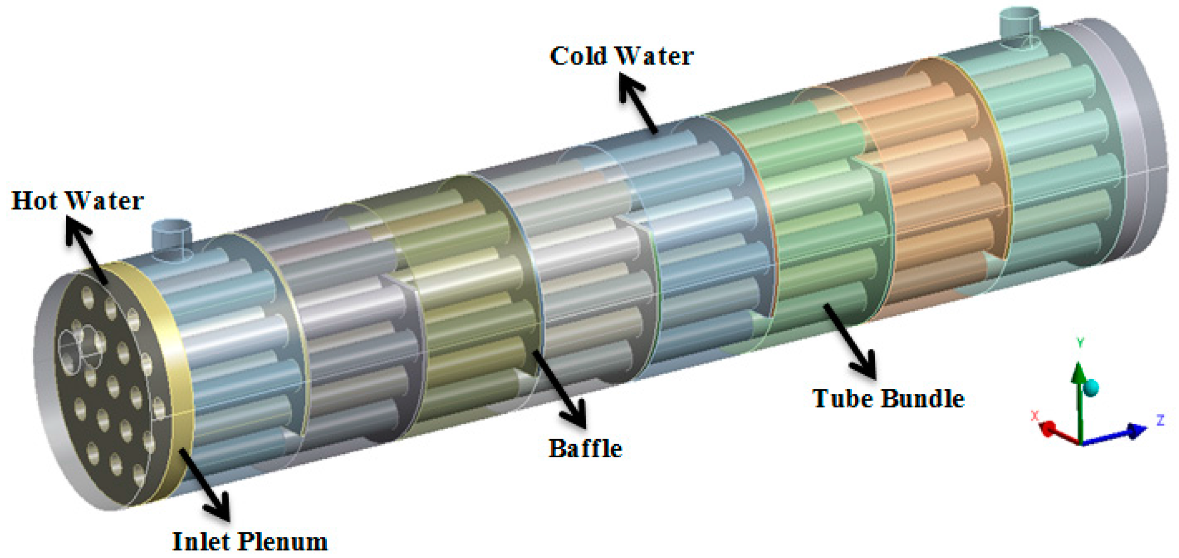
Figure 4.
CAD model of the shell and tube heat exchanger used in this numerical study.

Figure 5.
Separated fluid zones on the shell side of the heat exchanger.

Figure 6.
Mesh structure of the heat exchanger.

Figure 7.
Flow chart of numerical method for the desired solution of the thermal analysis of a shell and tube heat exchanger suggested in this study.
Figure 7.
Flow chart of numerical method for the desired solution of the thermal analysis of a shell and tube heat exchanger suggested in this study.

Figure 8.
Schematic view of section planes defined for comparative results for shell side.

Figure 9.
Window surfaces located between two adjacent fluid zones.

Figure 10.
Prediction of temperature (°C) distribution at section planes defined in shell side (Case-I).
Figure 10.
Prediction of temperature (°C) distribution at section planes defined in shell side (Case-I).

Figure 11.
Prediction of temperature (°C) distribution at section planes defined in shell side (Case-II).
Figure 11.
Prediction of temperature (°C) distribution at section planes defined in shell side (Case-II).

Figure 12.
Prediction of temperature (°C) distribution at section planes defined in shell side (Case-III).
Figure 12.
Prediction of temperature (°C) distribution at section planes defined in shell side (Case-III).

Figure 13.
Prediction of temperature (°C) distribution at section planes defined in shell side (Case-IV).
Figure 13.
Prediction of temperature (°C) distribution at section planes defined in shell side (Case-IV).

Figure 14.
Prediction of temperature (°C) distribution at section planes defined in shell side (Case-V).
Figure 14.
Prediction of temperature (°C) distribution at section planes defined in shell side (Case-V).

Figure 15.
Temperature distribution at the center plane of the heat exchanger (a) Case-I (b) Case-II (c) Case-III (d) Case-IV (e) Case-V.
Figure 15.
Temperature distribution at the center plane of the heat exchanger (a) Case-I (b) Case-II (c) Case-III (d) Case-IV (e) Case-V.

Figure 16.
Prediction of velocity (m s-1) distribution of shell side flow (a) Case-I (b) Case-II (c) Case-III (d) Case-IV (e) Case-V.
Figure 16.
Prediction of velocity (m s-1) distribution of shell side flow (a) Case-I (b) Case-II (c) Case-III (d) Case-IV (e) Case-V.


Table 1.
The dimensions of baffle spacing lengths for all cases.
| Spacing Length | Case-I (mm) | Case-II (mm) | Case-III (mm) | Case-IV (mm) | Case-V (mm) |
|---|---|---|---|---|---|
| L1 | 26.75 | 26.75 | 26.75 | 26.75 | 26.75 |
| L2 | 26.75 | 41.25 | 16.00 | 16.00 | 38.50 |
| L3 | 26.75 | 26.00 | 26.00 | 21.00 | 34.00 |
| L4 | 26.75 | 16.00 | 41.25 | 26.00 | 31.00 |
| L5 | 26.75 | 16.00 | 41.25 | 31.00 | 26.00 |
| L6 | 26.75 | 26.00 | 26.00 | 34.00 | 21.00 |
| L7 | 26.75 | 41.25 | 16.00 | 38.50 | 16.00 |
| L8 | 26.75 | 26.75 | 26.75 | 26.75 | 26.75 |
Table 2.
The dimensions of the shell side and tube side of the heat exchanger.
| Shell Side Dimensions | |
| Shell internal diameter | 44 mm |
| Shell wall thickness | 3 mm |
| Baffle plate wall thickness | 1 mm |
| Number of baffle plates | 7 |
| Tube Side Dimensions | |
| Tube internal diameter | 4 mm |
| Tube wall thickness | 1 mm |
| Effective tube length | 221 mm |
| Number of tubes in tube bundle | 19 |
Table 3.
Solver settings and boundary conditions used in the numerical simulations.
| Solver Settings | |
| Solver | Pressure-based |
| Time | Steady-state conditions |
| Equations | Combined simulation of flow and energy |
| Flow type | k-epsilon realizable turbulence model |
| Shell Side | |
| Supply temperature of cold water | 10 °C |
| Mass flow rate | 0.2 kg s−1 |
| Shell outer surfaces | Adiabatic conditions |
| Outlet nozzle | Gauge pressure equals to 0 Pa |
| Tube-Side | |
| Supply temperature of hot water | 50 °C |
| Mass flow rate | 0.3 kg s−1 |
| Outlet surfaces of the tube side | Gauge pressure equals to 0 Pa |
| Thermal Properties of Water at Mean Temperature | |
| Thermal conductivity | 0.6 W m−1 K−1 |
| Specific heat | Cold side: 4180 j kg−1 K−1 , Hot side: 4186.5 j kg−1 K−1 |
| Density | 998.2 kg m−3 |
| Dynamic viscosity | 0.001003 kg m−1 s−1 |
Table 4.
Computed temperature and pressure values at different surfaces (i).
| Surface Name | Case-I | Case-II | Case-III | |||
|---|---|---|---|---|---|---|
| Pressure (Pa) | Temperature (°C) | Pressure (Pa) | Temperature (°C) | Pressure (Pa) | Temperature (°C) | |
| Cold-inlet | 20,832 | 10.00 | 21,340 | 10.00 | 21,312 | 10.00 |
| Win-1 | 19,622 | 11.78 | 20,194 | 11.83 | 20,128 | 11.50 |
| Win-2 | 18,729 | 12.82 | 19,356 | 13.22 | 18,934 | 12.20 |
| Win-3 | 17,588 | 13.91 | 18,243 | 14.13 | 17,756 | 13.20 |
| Win-4 | 16,484 | 14.89 | 16,754 | 14.82 | 16,759 | 14.36 |
| Win-5 | 15,361 | 15.86 | 15,183 | 15.43 | 15,768 | 15.41 |
| Win-6 | 14,269 | 16.76 | 14,023 | 16.37 | 14,709 | 16.27 |
| Win-7 | 13,147 | 17.63 | 12,986 | 17.49 | 13,230 | 16.67 |
| Cold-outlet | 0 | 18.11 | 0 | 17.98 | 0 | 17.16 |
Table 5.
Computed temperature and pressure values at different surfaces (ii).
| Surface Name | Case-IV | Case-V | ||
|---|---|---|---|---|
| Pressure (Pa) | Temperature (°C) | Pressure (Pa) | Temperature (°C) | |
| Cold-inlet | 20,907 | 10.00 | 21,196 | 10.00 |
| Win-1 | 19,759 | 11.51 | 19,852 | 11.64 |
| Win-2 | 18,602 | 12.22 | 19,021 | 12.83 |
| Win-3 | 17,308 | 12.97 | 17,938 | 13.87 |
| Win-4 | 16,195 | 13.83 | 16,944 | 14.71 |
| Win-5 | 15,103 | 14.79 | 15,851 | 15.56 |
| Win-6 | 14,125 | 15.77 | 14,661 | 16.24 |
| Win-7 | 13,130 | 16.75 | 13,132 | 16.67 |
| Cold-outlet | 0 | 17.22 | 0 | 17.16 |
Table 6.
Predicted heat transfer rates on the shell side for all cases.
| Shell Side Fluid Zones | CFD Results of Heat Transfer Rates for All Cases (Watt) | ||||
|---|---|---|---|---|---|
| Case-I | Case-II | Case-III | Case-IV | Case-V | |
| Fluid zone-1 | 1460.59 | 1501.61 | 1230.83 | 1239.04 | 1345.71 |
| Fluid zone-2 | 853.38 | 1140.57 | 574.39 | 582.59 | 976.46 |
| Fluid zone-3 | 894.40 | 746.70 | 820.55 | 615.42 | 853.38 |
| Fluid zone-4 | 804.14 | 566.18 | 951.84 | 705.68 | 689.27 |
| Fluid zone-5 | 795.94 | 500.54 | 861.58 | 787.73 | 697.47 |
| Fluid zone-6 | 738.50 | 771.32 | 705.68 | 804.14 | 557.98 |
| Fluid zone-7 | 713.88 | 919.02 | 328.22 | 804.14 | 352.84 |
| Fluid zone-8 | 393.87 | 402.07 | 402.07 | 385.66 | 402.07 |
| Total | 6654.69 | 6548.02 | 5875.17 | 5924.40 | 5875.17 |
| Rh | 1 | 0.98 | 0.88 | 0.89 | 0.88 |
Table 7.
Results of numerical and analytical calculations for all cases.
| Heat Transfer Characteristics | |||||||
| Thermal properties | Case-I | Case-II | Case-III | Case-IV | Case-V | ||
| CFD | Kern | Bell-Delaware | CFD | ||||
| U (W m2 K−1) | 2533.06 | 2346.74 | 2269.00 | 2485.00 | 2175.54 | 2199.57 | 2177.83 |
| Qcold (W) | 6654.69 | 6164.72 | 5960.51 | 6548.02 | 5875.17 | 5924.40 | 5875.17 |
| Qhot (W) | 6654.18 | 6164.72 | 5960.51 | 6551.76 | 5871.48 | 5925.51 | 5876.63 |
| Pressure Drop Calculations | |||||||
| ΔPs (Pa) | CFD | Bell-Delaware | CFD | ||||
| 20,832 | 17,769 | 21,340 | 21,312 | 20,907 | 21,196 | ||
Table 8.
CFD results of velocity distribution for each fluid zone (m/s).
| Shell Side Fluid Zones | Case-I | Case-II | Case-III | Case-IV | Case-V |
|---|---|---|---|---|---|
| Fluid zone-1 | 0.62 | 0.62 | 0.62 | 0.62 | 0.62 |
| Fluid zone-2 | 0.44 | 0.37 | 0.61 | 0.60 | 0.37 |
| Fluid zone-3 | 0.50 | 0.50 | 0.52 | 0.57 | 0.46 |
| Fluid zone-4 | 0.50 | 0.65 | 0.41 | 0.52 | 0.46 |
| Fluid zone-5 | 0.49 | 0.66 | 0.40 | 0.47 | 0.50 |
| Fluid zone-6 | 0.50 | 0.52 | 0.50 | 0.44 | 0.55 |
| Fluid zone-7 | 0.49 | 0.41 | 0.65 | 0.41 | 0.66 |
| Fluid zone-8 | 0.58 | 0.57 | 0.59 | 0.57 | 0.59 |
| Average | 0.51 | 0.51 | 0.51 | 0.51 | 0.51 |
© 2017 by the authors. Licensee MDPI, Basel, Switzerland. This article is an open access article distributed under the terms and conditions of the Creative Commons Attribution (CC BY) license (http://creativecommons.org/licenses/by/4.0/).
Share and Cite
MDPI and ACS Style
Bayram, H.; Sevilgen, G. Numerical Investigation of the Effect of Variable Baffle Spacing on the Thermal Performance of a Shell and Tube Heat Exchanger. Energies 2017, 10, 1156. https://doi.org/10.3390/en10081156
AMA Style
Bayram H, Sevilgen G. Numerical Investigation of the Effect of Variable Baffle Spacing on the Thermal Performance of a Shell and Tube Heat Exchanger. Energies. 2017; 10(8):1156. https://doi.org/10.3390/en10081156
Chicago/Turabian StyleBayram, Halil, and Gökhan Sevilgen. 2017. "Numerical Investigation of the Effect of Variable Baffle Spacing on the Thermal Performance of a Shell and Tube Heat Exchanger" Energies 10, no. 8: 1156. https://doi.org/10.3390/en10081156
Note that from the first issue of 2016, this journal uses article numbers instead of page numbers. See further details here.