Numerical Simulation of Density-Driven Flow and Heat Transport Processes in Porous Media Using the Network Method

Abstract

Density-driven flow and heat transport processes in 2-D porous media scenarios are governed by coupled, non-linear, partial differential equations that normally have to be solved numerically. In the present work, a model based on the network method simulation is designed and applied to simulate these processes, providing steady state patterns that demonstrate its computational power and reliability. The design is relatively simple and needs very few rules. Two applications in which heat is transported by natural convection in confined and saturated media are studied: slender boxes heated from below (a kind of Bénard problem) and partially heated horizontal plates in rectangular domains (the Elder problem). The streamfunction and temperature patterns show that the results are coherent with those of other authors: steady state patterns and heat transfer depend both on the Rayleigh number and on the characteristic Darcy velocity derived from the values of the hydrological, thermal and geometrical parameters of the problems.

1. Introduction

The topic of density-driven flow in porous media has aroused great interest among researchers in the last decades. The solution patterns of the complex phenomena involved in these processes are fundamental for the exploitation of geothermal energy extraction systems (Cheng [1]; Revil et al. [2]; Pruess [3]; Ciriello et al. [4]; Böttcher et al. [5]). In addition, other subjects such as saltwater intrusion, underground spreading of pollutants, thermal insulation or petroleum engineering also involve the fundamentals of density-driven flow in porous media (Liu et al. [6]; Adler [7]).

Fluid flow and heat transport processes in porous media are governed by coupled, non-linear PDEs derived from momentum and mass and energy conservation laws. The pioneering works in this field were conducted by Horton and Rogers [8], Lapwood [9] and Wooding [10], who addressed the porous medium analog of Bénard convection with regard to thermal instability in a saturated porous layer of infinite horizontal extent. Elder [11,12] performed laboratory experiments with Hele–Shaw cells and computed 2-D convection patterns for both transient and steady-state using a finite-difference method. Since then, the numbers of works on this topic has increased considerably; in this sense, excellent reviews of these problems can be found in Holzbecher [13], Vafai [14], Diersch and Kolditz [15], Bejan et al. [16] and Nield and Bejan [17].

As subsequent studies began to cover new subjects, the importance of numerical analysis soon became apparent and different techniques were applied: finite-differences, finite-volumes, finite-elements, Garlekin technique and lattice Boltzmann method (Straus [18]; Hickox and Gartling [19]; Debéda et al. [20]; Šarler et al. [21]). Moreover, the steady-state patterns of temperature and streamfunction related to the different scenarios that emerge in these problems, as well as their stability, are also of interest due to these patterns not only provide a clear insight into the coupled phenomena involved, but they can also be used for testing the numerical codes proposed for the solution.

In this paper, the network method is proposed to simulate density-driven flow and heat transport processes in porous media. In recent years, this numerical technique has been successfully applied to a great number of problems in different fields of engineering and science, such as electrochemistry, heat transfer, tribology, where it has provided accurate solutions in all cases (Morales et al. [22]; Caravaca et al. [23]; Sánchez-Pérez et al. [24]; Marín et al. [25]). The network method, whose application follows formal steps that require few programming rules, makes good use of the powerful computational algorithms integrated in modern circuit simulation codes, allowing the exact solution of the model and reducing the errors to the size of the mesh grid.

To demonstrate the reliability of the network method, two selected applications, in which heat transports by natural convection in confined and saturated porous media, are chosen to demonstrate the reliability and robustness of the proposed method: slender boxes heated from below (a kind of Bénard problem, Holzbecher [13]) and partially heated horizontal plates in rectangular domains (the Elder problem, Elder [11,12]). Despite the simplicity of the boundary conditions, both problems can be assumed as benchmarks for testing purposes. The choice of these two applications is based on the significant differences in their resulting patterns. In slender box, the emergent eddy covers the whole domain with a high degree of symmetry, while temperature is evenly distributed; in contrast, the distorted eddy of the Elder problem gives rise to large velocities in the region nearest the thermal focus and large temperature gradients in part of the top and bottom boundaries.

2. Steady-State Governing Equations and Boundary Conditions for a 2-D Domain

Figure 1 depicts the physical scenario of the two selected applications. The left-hand scenario (Figure 1a) refers to a slender box with a height greater than the length of the base, while, in the right-hand scenario (Figure 1b), the length is greater than the height and the bottom plate is partially heated in its center region. A porous medium assumes thermal and hydraulic anisotropic properties. Finally, Boussinesq approximation is assumed since this hypothesis is widely used in most processes in this field.

The set of steady state governing equations is formed by the momentum (Darcy’s law), the mass conservation and energy equations. For an anisotropic 2-D medium, using the rectangular coordinates of Figure 1, Darcy´s law is written in the form:

$$\mathrm{u}=-\left(\frac{{\mathrm{K}}_{\mathrm{x}}}{\mathsf{\mu }}\right)\left(\frac{\partial \mathrm{P}}{\partial \mathrm{x}}\right),\mathrm{v}=-\left(\frac{{\mathrm{K}}_{\mathrm{y}}}{\mathsf{\mu }}\right)\left[\left(\frac{\partial \mathrm{P}}{\partial \mathrm{y}}\right)+\mathsf{\rho }\mathrm{g}\right]$$

(1)

These equations can be merged by eliminating the pressure. Doing this, and taking into account the Boussinesq approximation, ∆$\mathsf{\rho }=-{\mathsf{\rho }}_0\mathsf{\beta }\left(∆\mathrm{T}\right)$, the momentum equation is reduced to:

$$\left(\frac{{\mathrm{K}}_{\mathrm{y}}}{{\mathrm{K}}_{\mathrm{x}}}\right)\left(\frac{\partial \mathrm{u}}{\partial \mathrm{y}}\right)-\left(\frac{\partial \mathrm{v}}{\partial \mathrm{x}}\right)=-\left(\frac{{\mathsf{\rho }}_0{\mathrm{K}}_{\mathrm{y}}\mathrm{g}\mathsf{\beta }}{\mathsf{\mu }}\right)\left(\frac{\partial \mathrm{T}}{\partial \mathrm{x}}\right)$$

(2)

In addition, mass and energy conservation equations are expressed as:

$$\left(\frac{\partial \mathrm{u}}{\partial \mathrm{x}}\right)+\left(\frac{\partial \mathrm{v}}{\partial \mathrm{y}}\right)=0$$

(3)

$$\left({\mathsf{\rho }}_{\mathrm{f}}{\mathrm{c}}_{\mathrm{p},\mathrm{f}}\right)\mathrm{u}\left(\frac{\partial \mathrm{T}}{\partial \mathrm{x}}\right)+\left({\mathsf{\rho }}_{\mathrm{f}}{\mathrm{c}}_{\mathrm{p},\mathrm{f}}\right)\mathrm{v}\left(\frac{\partial \mathrm{T}}{\partial \mathrm{y}}\right)={\mathrm{k}}_{\mathrm{m},\mathrm{x}}\left(\frac{{\partial }^2\mathrm{T}}{\partial {\mathrm{x}}^2}\right)+{\mathrm{k}}_{\mathrm{m},\mathrm{y}}\left(\frac{{\partial }^2\mathrm{T}}{\partial {\mathrm{y}}^2}\right)$$

(4)

The average thermal conductivity depends on the solid and fluid portions of the porous medium and on their respective conductivities: This dependence in terms of porosity can be written as ${\mathrm{k}}_{\mathrm{m}}=\left[\mathsf{\varphi }{\mathrm{k}}_{\mathrm{f}}+\left(1-\mathsf{\varphi }\right){\mathrm{k}}_{\mathrm{s}}\right]$.

For a better illustration of the graphic solutions, a potential scalar function from which the velocity can be derived, the streamfunction variable (ψ), is used as the dependent variable instead of velocity. This has the advantage that the isolines of ψ directly show the way in which the particles of fluid move. The connection between velocity and streamfunction variables is given by the partial derivative expressions “u = ∂ψ/∂y” and “v = −∂ψ/∂x”.

To complete the mathematical models, the following boundary conditions are assumed:

(i)

Vertical slender boxes (Figure 1, left):

$${\mathrm{T}}_{\left(\mathrm{x},\mathrm{y}=0\right)}=1,{\mathrm{T}}_{\left(\mathrm{x},\mathrm{y}=\mathrm{H}\right)}=0,{\left(\frac{\partial \mathrm{T}}{\partial \mathrm{x}}\right)}_{\left(\mathrm{x}=0,\mathrm{y}\right)}={\left(\frac{\partial \mathrm{T}}{\partial \mathrm{x}}\right)}_{\left(\mathrm{x}=\mathrm{L},\mathrm{y}\right)}=0$$

(5a)

$${\mathsf{\psi }}_{\left(\mathrm{x},\mathrm{y}=0\right)}={\mathsf{\psi }}_{\left(\mathrm{x},\mathrm{y}=\mathrm{H}\right)}={\mathsf{\psi }}_{\left(\mathrm{x}=0,\mathrm{y}\right)}={\mathsf{\psi }}_{\left(\mathrm{x}=\mathrm{L},\mathrm{y}\right)}=0$$

(5b)

(ii)

Elder problem (Figure 1, right):

$$\begin{gathered} {\mathrm{T}}_{\left(\mathrm{a}<\mathrm{x}<\mathrm{L}-\mathrm{a},\mathrm{y}=0\right)}=1,{\mathrm{T}}_{\left(\mathrm{x},\mathrm{y}=\mathrm{H}\right)}=0, \\ {\left(\frac{\partial \mathrm{T}}{\partial \mathrm{x}}\right)}_{\left(0<\mathrm{x}<\mathrm{a},\mathrm{y}=0\right)}={\left(\frac{\partial \mathrm{T}}{\partial \mathrm{x}}\right)}_{\left(\mathrm{L}-\mathrm{a}<\mathrm{x}<\mathrm{L},\mathrm{y}=0\right)}={\left(\frac{\partial \mathrm{T}}{\partial \mathrm{x}}\right)}_{\left(\mathrm{x}=0,\mathrm{y}\right)}={\left(\frac{\partial \mathrm{T}}{\partial \mathrm{x}}\right)}_{\left(\mathrm{x}=\mathrm{L},\mathrm{y}\right)}=0 \end{gathered}$$

(6a)

$${\mathsf{\psi }}_{\left(\mathrm{x},\mathrm{y}=0\right)}={\mathsf{\psi }}_{\left(\mathrm{x},\mathrm{y}=\mathrm{H}\right)}={\mathsf{\psi }}_{\left(\mathrm{x}=0,\mathrm{y}\right)}={\mathsf{\psi }}_{\left(\mathrm{x}=\mathrm{L},\mathrm{y}\right)}=0$$

(6b)

The aspect ratio of the problem L/H is smaller than unity in the first case (i) but greater than unity in the second case (ii).

3. The Network Model

As mentioned in the Introduction, during recent years, the network method has been successfully applied to a great variety of problems in science and engineering. Soto-Meca et al. [26] applied this technique to simulate fluid flow and solute transport. In this sense, part of the model is similar, since the topics “fluid flow and solute transport” and “fluid flow and heat transport” have one common part: the governing equation related to momentum (Equation (2)). However, there are important differences relating to the software that specifies each of the electrical devices that implement the “heat transport” section of the model (Figure 2b) and to the electrical devices of boundary conditions. Besides, the thermal parameters involved in “heat transport” have specific expressions (mean values) different from those of the parameters involved in “solute transport”.

Application of the network method follows two clear stages: (i) design (for which the programmer must have some knowledge of convectional circuit theory); and (ii) simulation in an appropriate software such as PSPICE [27]. In addition, the potential convergence and stability problems that arise in numerical simulations are solved by adjusting a parameter that reflects a compromise between the computing time and the accuracy of the solution. Another advantage of the method is that, since the codes of circuit simulation must satisfy Kirchhoff’s theorems (one of which refers to electric current conservation and the other to electric potential unicity), the errors produced in other methods by neglecting the differences in the balance of input and output flows in each volume element do not arise. The code adjusts the numerical calculation to provide a solution in which these differences are negligible. The user requires no other mathematical manipulations (González-Fernández and Alhama [28]).

The network model can be considered as a representation of the natural convection problem. In the network method, the coupled PDEs that govern the problem are reduced to finite-difference differential equations by discretizing the spatial independent variables, while time is retained as a continuous variable. The network model is designed assuming that the addends of each equation are electric currents that balance each other in the principal node of the circuit—in the same way that physical quantities that counteract each other in the equation do so in the physical domain of the volume element. There are as many circuits as governing equations.

Thus, each addend is implemented in its respective branch by an electric device, whose constitutive equation is the mathematical expression of the addend in question. The addends that realize the coupling between equations are also easily implemented by a special kind of device, called a controlled source, which provides an output current specified as an arbitrary mathematical function, whose arguments can be voltages and/or currents at any point or any device of the network. Besides, network cells are inter-connected by ideal electrical contacts to form the whole model of the domain. Boundary conditions are finally also implemented by means of electrical devices.

The equivalence between thermal and electric variables is implemented as follows:

• j (electric current, W/m²)—heat flux density (W/m²)
• V (electric potential, V)—temperature (K)

for the heat transport circuit, and:

• j (electric current, W/m²)—flow velocity (m/s)
• V (electric potential, V)—streamfunction variable (m²/s)

for the fluid flow circuit. The equations from which the model is designed are the finite-difference differential equations derived from those of momentum and energy, Equations (2) and (4), respectively; the energy equation, written in terms of streamfunction and temperature, is:

$$\left(\frac{{\mathrm{K}}_{\mathrm{y}}}{{\mathrm{K}}_{\mathrm{x}}}\right)\left(\frac{{\partial }^2\mathsf{\psi }}{\partial {\mathrm{y}}^2}\right)+\left(\frac{{\partial }^2\mathsf{\psi }}{\partial {\mathrm{x}}^2}\right)=-\left(\frac{{\mathsf{\rho }}_0{\mathrm{K}}_{\mathrm{y}}\mathrm{g}\mathsf{\beta }}{\mathsf{\mu }}\right)\left(\frac{\partial \mathrm{T}}{\partial \mathrm{x}}\right)$$

(7)

$$\left({\mathsf{\rho }}_{\mathrm{f}}{\mathrm{c}}_{\mathrm{p},\mathrm{f}}\right)\left(\frac{\partial \mathsf{\psi }}{\partial \mathrm{y}}\right)\left(\frac{\partial \mathrm{T}}{\partial \mathrm{x}}\right)-\left({\mathsf{\rho }}_{\mathrm{f}}{\mathrm{c}}_{\mathrm{p},\mathrm{f}}\right)\left(\frac{\partial \mathsf{\psi }}{\partial \mathrm{x}}\right)\left(\frac{\partial \mathrm{T}}{\partial \mathrm{y}}\right)={\mathrm{k}}_{\mathrm{m},\mathrm{x}}\left(\frac{{\partial }^2\mathrm{T}}{\partial {\mathrm{x}}^2}\right)+{\mathrm{k}}_{\mathrm{m},\mathrm{y}}\left(\frac{{\partial }^2\mathrm{T}}{\partial {\mathrm{y}}^2}\right)$$

(8)

which, in finite-difference form, referring to a volume element, and using the nomenclature of Figure 2, can be conveniently written as:

$$\begin{array}{c}\frac{1}{∆\mathrm{y}}{\left(\frac{∆\mathsf{\psi }}{\left(\frac{{\mathrm{K}}_{\mathrm{x}}}{{\mathrm{K}}_{\mathrm{y}}}\right)\left(\frac{∆\mathrm{y}}{2}\right)}\right)}_{\mathrm{out}}-\frac{1}{∆\mathrm{y}}{\left(\frac{∆\mathsf{\psi }}{\left(\frac{{\mathrm{K}}_{\mathrm{x}}}{{\mathrm{K}}_{\mathrm{y}}}\right)\left(\frac{∆\mathrm{y}}{2}\right)}\right)}_{\mathrm{in}}+\frac{1}{∆\mathrm{x}}{\left(\frac{∆\mathsf{\psi }}{\left(\frac{∆\mathrm{x}}{2}\right)}\right)}_{\mathrm{out}}-\frac{1}{∆\mathrm{x}}{\left(\frac{∆\mathsf{\psi }}{\left(\frac{∆\mathrm{x}}{2}\right)}\right)}_{\mathrm{in}}\hfill \\ =-\left(\frac{{\mathsf{\rho }\mathrm{K}}_{\mathrm{y}}\mathrm{g}\mathsf{\beta }}{\mathsf{\mu }}\right)\left(\frac{∆\mathrm{T}}{∆\mathrm{x}}\right)\hfill \end{array}$$

(9)

$$\begin{array}{c}\left({\mathsf{\rho }}_{\mathrm{f}}{\mathrm{c}}_{\mathrm{p},\mathrm{f}}\right)\left[\left(\frac{∆\mathsf{\psi }}{∆\mathrm{y}}\right)\left(\frac{∆\mathrm{T}}{∆\mathrm{x}}\right)-\left(\frac{∆\mathsf{\psi }}{∆\mathrm{x}}\right)\left(\frac{∆\mathrm{T}}{∆\mathrm{y}}\right)\right]=\hfill \\ \frac{1}{∆\mathrm{x}}{\left(\frac{∆\mathrm{T}}{\left(\frac{∆\mathrm{x}}{2{\mathrm{k}}_{\mathrm{m},\mathrm{x}}}\right)}\right)}_{\mathrm{out}}-\frac{1}{∆\mathrm{x}}{\left(\frac{∆\mathrm{T}}{\left(\frac{∆\mathrm{x}}{2{\mathrm{k}}_{\mathrm{m},\mathrm{x}}}\right)}\right)}_{\mathrm{in}}+\frac{1}{∆\mathrm{y}}{\left(\frac{∆\mathrm{T}}{\left(\frac{∆\mathrm{y}}{2{\mathrm{k}}_{\mathrm{m},\mathrm{y}}}\right)}\right)}_{\mathrm{out}}-\frac{1}{∆\mathrm{y}}{\left(\frac{∆\mathrm{T}}{\left(\frac{∆\mathrm{y}}{2{\mathrm{k}}_{\mathrm{m},\mathrm{y}}}\right)}\right)}_{\mathrm{in}}\hfill \end{array}$$

(10)

Each term of each equation is an electric current variable, which is balanced in the volume element by the other terms depending on its sign. Each equation, in turn, gives rise to an independent network, which is 2-D connected to adjoining circuits to make up the whole scenario. These equations can be considered as Kirchhoff´s current law at the (i, j) node—the center of the volume element—for the flow velocity and heat flux variables, respectively. The lineal fluid flow and temperature terms, to which Ohm’s law can be directly applied, are implemented in the model by simple resistors, and the values of which are:

$${\mathrm{R}}_{\mathsf{\psi },\mathrm{y},\mathrm{out}}={\mathrm{R}}_{\mathsf{\psi },\mathrm{y},\mathrm{in}}=\left(\frac{{\mathrm{K}}_{\mathrm{x}}}{{\mathrm{K}}_{\mathrm{y}}}\right)\frac{{\left(∆\mathrm{y}\right)}^2}{2},{\mathrm{R}}_{\mathsf{\psi },\mathrm{x},\mathrm{out}}={\mathrm{R}}_{\mathsf{\psi },\mathrm{x},\mathrm{in}}=\frac{{\left(∆\mathrm{x}\right)}^2}{2}$$

(11a)

$${\mathrm{R}}_{\mathrm{T},\mathrm{y},\mathrm{out}}={\mathrm{R}}_{\mathrm{T},\mathrm{y},\mathrm{in}}=\left(\frac{{\left(∆\mathrm{y}\right)}^2}{2{\mathrm{k}}_{\mathrm{m},\mathrm{y}}}\right),{\mathrm{R}}_{\mathrm{T},\mathrm{x},\mathrm{out}}={\mathrm{R}}_{\mathrm{T},\mathrm{x},\mathrm{in}}=\left(\frac{{\left(∆\mathrm{x}\right)}^2}{2{\mathrm{k}}_{\mathrm{m},\mathrm{x}}}\right)$$

(11b)

while the non-linear terms j_ψ,∆Tx, j_T,∆ψx and j_T,∆ψy, for the momentum and energy equations, respectively, are implemented by controlled current sources, whose output current is specified by programming. In Figure 2, G_Ψ implements the current terms j_ψ,∆Tx, while G_T,x and G_T,y do so for the currents j_T,∆ψx and j_T,∆ψy, respectively.

A total number of N × M volume elements are connected in series to represent the whole domain. The electrical devices necessary for the implementation of the Dirichlet and Neumann boundary conditions are a constant voltage source and resistor of very high (infinite) value, respectively. It is important to mention that other kinds of boundary conditions are easily implemented using controlled current (or voltages) sources. Once these conditions are implemented, the network model is complete.

As regards simulation of the network, two options can be followed to introduce the model in the simulation code PSPICE. The first involves a text file of the model, for which few programming rules are used (rules for the specification of the resistors and sources plus standard sentences referring to the grid size and to the kind and accuracy of the analysis), while the second involves the use of a symbolic language by means of the “schematics” option of PSPICE.

4. Applications

The complete network model is formed by 20 (horizontal) × 80 (vertical) identical rectangular volume elements for the first application (slender boxes) and 80 (horizontal) × 20 (vertical) for the second application (Elder´s problem), according to their relative aspect ratio. Once the model has been simulated, output data are read and treated by Matlab [29] routines for their representation since the output graphic ambient of PSPICE, the code simulator, is not appropriate for showing 2-D patterns.

All the simulations reported reach a stable steady state, following the criterion that the numerical solution does not change within the last time step. The main parameters that control the simulation in PSPICE are: (i) the relative tolerance, an accuracy criterion chosen by the user; and (ii) the time step. The last, which satisfies the Courant criterion, can be changed during the simulation, depending on the smoothness of the solution to reduce the total computing time.

Since both problems are ruled by the same governing equations, they have may aspects in common. However, from the point of view of their solution, the problems can be considered clearly different. While the Elder problem is characterized by a constant Rayleigh number of 400 (a value for which the convection has been completely developed), a wide range of values for Rayleigh (200, 300 and 400) is assumed for slender boxes. Another difference between the problems refers to the aspect of their patterns. In slender boxes there is complete symmetry in the eddy that emerges and covers the whole domain, while temperature isolines are regularly distributed from the bottom to the top boundaries. In contrast, the stable eddy that appears in the Elder problem is asymmetric, the greatest velocities concentrating in the region nearest to the source of heat, while temperature isolines have an irregular distribution, the steep gradients of this variable concentrating in the right side of the top and bottom boundaries.

4.1. Slender Boxes Heated from Below

The physical scheme of this problem is shown in Figure 1a. This is a kind of Bénard problem (Bénard [30]) but with a different aspect ratio, since the height of the domain is greater than its length. Bénard’s original experiment in 1900, which refers to a rectangle of large aspect ratio L (length)/H (height) = 100, provides a steady state solution pattern organized in regular cells (Bénard cells) of a constant length. However, for slender boxes of aspect ratio smaller than unity, the steady state pattern is formed by one symmetric flow eddy, in which heat is transferred by conduction near the top and bottom, where temperature isolines of the pattern are horizontal, and by convection in the core cell, where the isolines tend to be vertical. The onset of convection in all scenarios takes place when the Rayleigh number (Ra) is larger than a critical threshold value. According to Holzbecher [13], steady state temperature and streamfunction patterns only depend on Ra.

The geometrical domain is given by L (width) = 90 m and H (height) = 360 m. Three cases with different Darcy velocities, v_D, but constant Rayleigh number, Ra, are studied. To check the reliability of the network method, the change in the individual parameters for each case is noticeable—even when values of gravitational acceleration are not representative of natural environments. These large deviations would mean that the Boussinesq approximation is not applicable but the test in question does not depend on this approximation: for the same governing equations, patterns must be identical for the same Ra. The hydrogeological parameters of the chosen cases are shown in

Table 1. Physical parameters of the first application.

Case	K (m2)	α (m2/s)	μ (kg/m∙s)	∆⍴ (kg/m3)	g (m/s2)	vD (m/s)	Ra
1	4.831 × 10−14	1.0 × 10−6	2.0 × 10−4	230	9.81	5.452 × 10−7	200
2	9.662 × 10−14	2.0 × 10−6	4.0 × 10−4	115	9.81	1.09 × 10−6	200
3	1.449 × 10−13	3.0 × 10−6	8.0 × 10−4	460	19.62	1.635 × 10−6	200

. The Darcy velocity and Ra number are given by the expressions:

$${\mathrm{v}}_{\mathrm{D}}=\left(\frac{\mathrm{K}}{\mathsf{\mu }}\right)\left(∆\mathsf{\rho }\right)\mathrm{g},\mathrm{Ra}=\left(\frac{\mathrm{Kg}∆\mathsf{\rho }\mathrm{H}}{\mathsf{\mu }\mathsf{\alpha }}\right)$$

(12)

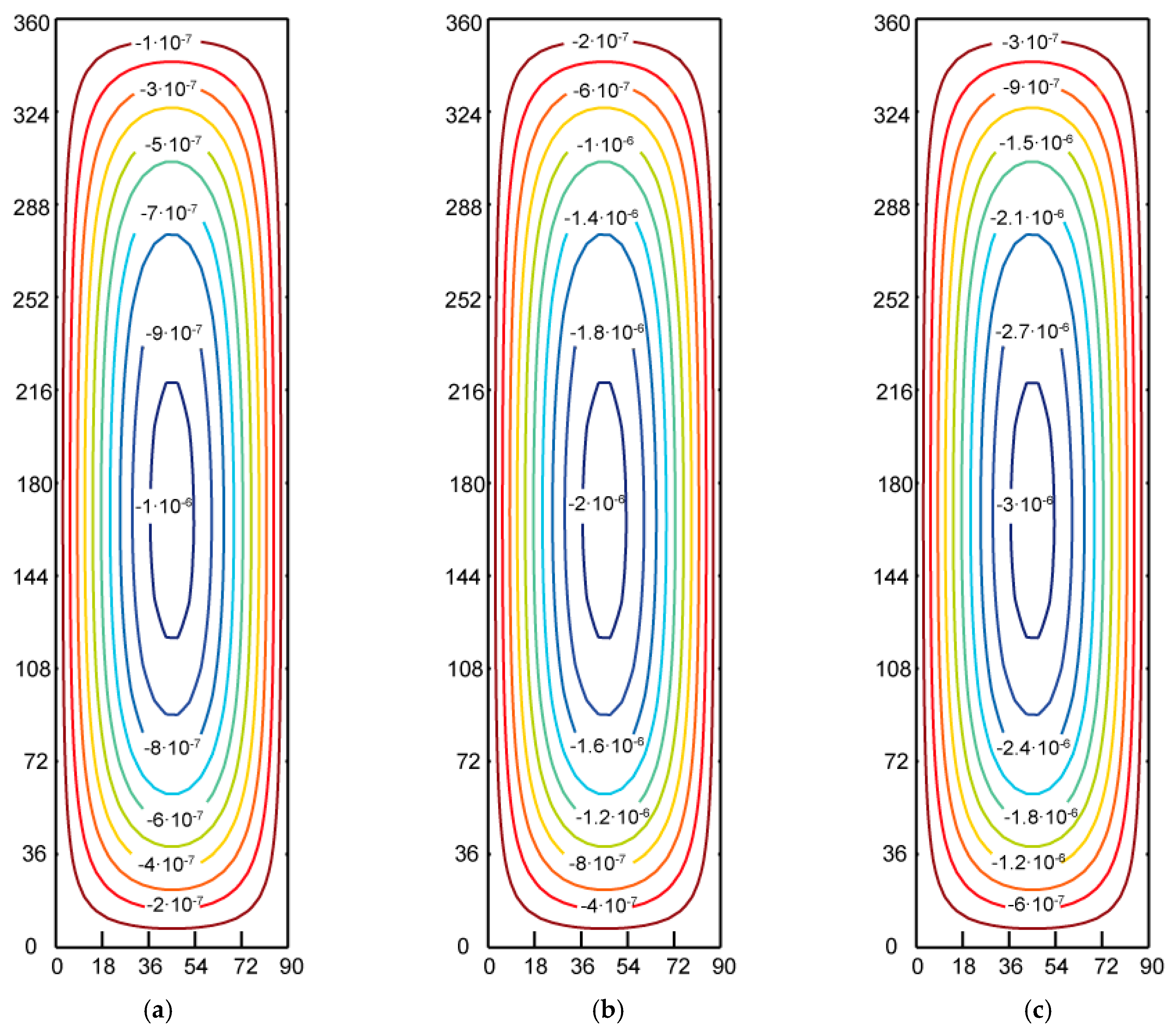
Figure 3 shows the temperature patterns of the three cases for a grid of 1600 cells, 20 (horizontal) × 80 (vertical). As shown, these patterns are quite similar despite the appreciable differences between some parameters. Temperature isolines are regularly distributed along the vertical domain and show an inverse symmetry, providing greater thermal gradients near the center of vertical boundaries and smaller gradients at the center of the horizontal boundaries. Figure 4 shows the expected steady state patterns of ψ. Values of ψ isolines for each case were chosen in such a way that water flow as seen in the figure (difference between the ψ-values of adjacent lines divided by the distance between them), can be easily compared.

Figure 5 shows a comparison of the network solution with that provided by Holzbecher [13], who used the software FAST-C(2D) based on the finite difference numerical technique, using the same mesh grid, 20 (horizontal) × 80 (vertical). Results are very close for the three Ra values, providing maximum deviations in the order of 5%.

Finally, a sensitivity analysis related with the vertical grid size is depicted in Figure 6 for Ra 200, 300 and 400. The deviations for a small grid (20 × 20) compared with a large grid (20 × 80) are negligible, probably due to the precise interpolation of Matlab routines used for the representation. For a better appreciation,

Table 2. Deviations in the sensitivity analysis for Ra = 300.

x-Locations	Mesh (Cells)	20 × 20 (400)	50 × 20 (1000)	60 × 20 (1200)	72 × 20 (1440)	80 × 20 (1600)
x = L/4	y (T’ = 0.2)	304.2	307.8	307.8	307.8	309.6
	y (T’ = 0.6)	49	46.8	48.6	48.6	45
x = L/2	y (T’ = 0.2)	334.8	336.6	336.6	336.6	338
	y (T’ = 0.6)	106.2	108	108	108	109.8
x = 3L/4	y (T’ = 0.2)	342	343.8	343.8	343.8	345.6
	y (T’ = 0.6)	174.6	176.4	178.2	178.2	178.2

gives numerical data of the sensitivity analysis. For two typical isotherms (T = 0.2 and 0.6) and three horizontal locations (x = L/4, L/2 and 3L/4), the vertical location is read from the solution. As can be seen, the deviations are negligible.

Computing time simulations for the higher grid size is in the order of 300 s, most of which is required by the data treatment and graphical representation routines.

4.2. Horizontal Plates in Saturated Domain Partially Heated from Below (the Elder Problem)

The physical scheme of this application is shown in Figure 1b. The problem originally proposed by Elder [11,12] for scenarios of solute transport as well as for heat transport uses different boundary conditions. Elder’s experiment is somewhat similar to Bénard´s, but chooses a distribution where the system is only partially heated from below (half of the lower boundary). An excellent autobiographical and biographical historical account of the genesis, evolution and resolution can be found in Elder et al. [31]. Using the streamfunction formulation and normalized temperature variables for a 2-D domain, Elder presented the first numerical simulation of the laboratory set-up in the same publication. On the one hand, steady state patterns of flow are formed by a number of eddies that depend on the Rayleigh number and on the ratio between the heated part of the bottom boundary and its length. On the other hand, temperature patterns clearly show the predominant type of heat transfer existing in the domain—conduction near the horizontal isothermal boundaries and convection in the rest. As in the first application, the dimensionless parameter that characterizes the solution patterns (for the same ratio between the lengths of thermal focus and horizontal domain) is the Rayleigh number, Holzbecher [13].

The geometrical domain is given by L (width) = 600 m, H (height) = 150 m and b = 300 m. The physical parameters are listed in

Table 3. Physical parameters of the second application.

Case	K (m2)	α (m2/s)	μ (kg/m∙s)	∆⍴ (kg/m3)	g (m/s2)	vD (m/s)	Ra
1	4.85 × 10−13	3.565 × 10−7	1.0 × 10−3	200	9.81	9.506 × 10−10	400
2	9.69 × 10−13	7.13 × 10−7	2.0 × 10−3	400	9.81	1.901 × 10−9	400

for the two cases chosen. As in the former application, the Rayleigh number retains the same value, Ra = 400, while the Darcy velocity in Case 2 is twice that of Case 1 due to the parameter values. Simulations can be carried out for half of the domain due to the symmetry involved in the problem.

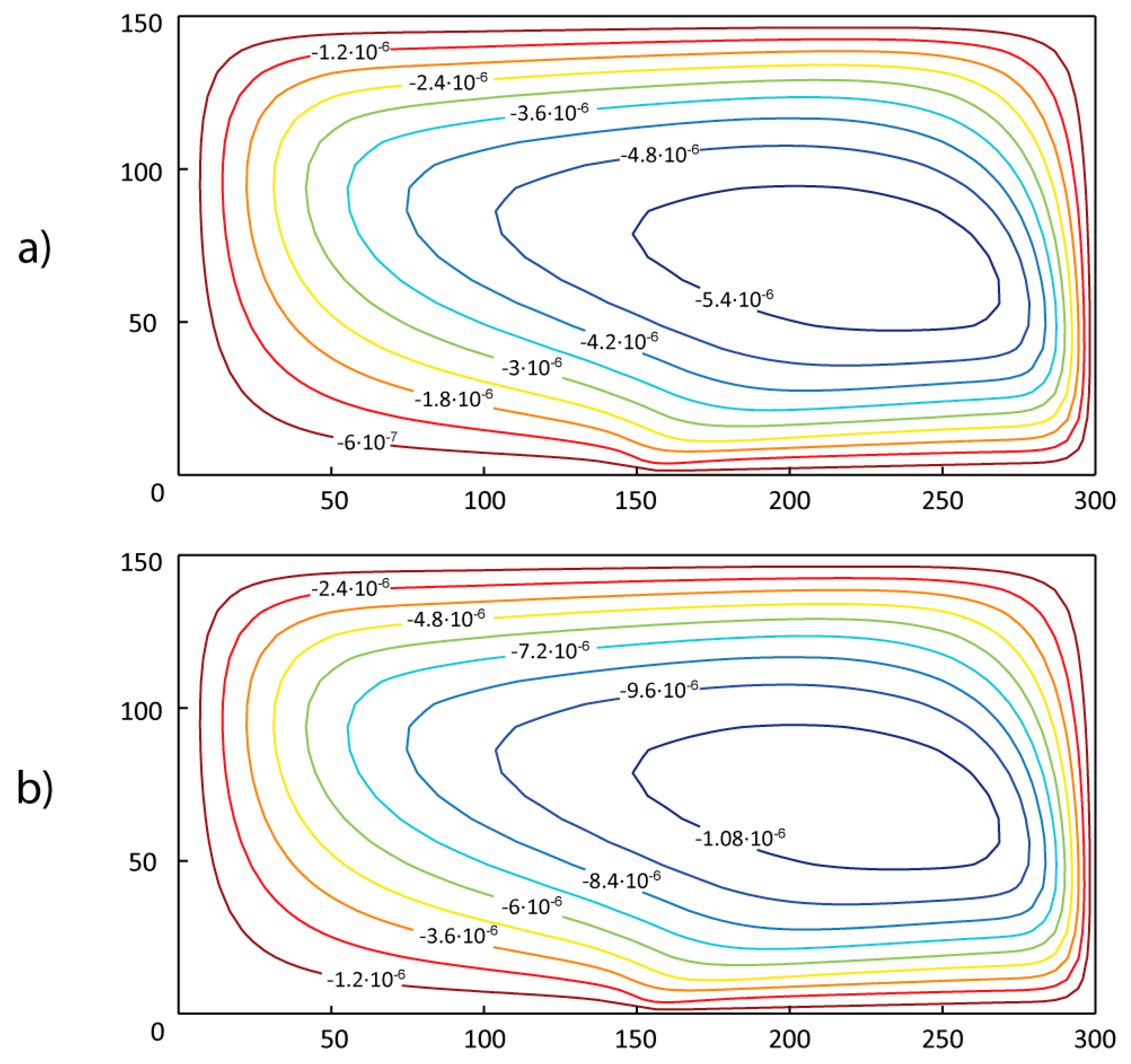
Figure 7 and Figure 8 depict the temperature and streamfunction patterns, respectively, for Cases 1 and 2 of Table 3, using a grid size of 80 (horizontal) × 20 (vertical) cells. Values of ψ are chosen to facilitate water flow readings. As expected, simulations provide the same results. In contrast with the slender box, where temperature isolines are regularly distributed from the bottom to the top boundaries, the Elder pattern defines an irregular distribution that concentrates the isolines (or the temperature gradients) on the right of the top and bottom boundaries. These lines, in turn, become increasingly separated as the distance from the thermal focus increases. As regards the streamfunction, only one eddy covering the whole domain emerges, with no symmetry; isolines of ψ are concentrated on the right side of the domain—the region with high velocities—and are more separate in the rest of the domain. Note that water flow in all regions of the domain for Case 2 is double the resulting flow of Case 1 in the same regions; this agrees with the relative value of Darcy´s velocity for both cases.

Comparison of network and Elder simulations is carried out in

Table 4. Comparison of network method and Elder solutions for the isolines of temperature 0.2 and 0.6.

Temperature	Elder		Network Method
	x’	y’	y’
T’ = 0.2	0.9	0.96	0.97
	0.8	0.96	0.96
	0.7	0.95	0.95
	0.6	0.95	0.94
	0.5	0.94	0.92
	0.4	0.93	0.89
	0.3	0.83	0.84
T’ = 0.6	0.95	0.89	0.91
	0.9	0.86	0.87
	0.8	0.76	0.78

. For two typical temperature isolines (T = 0.2 and 0.6), and regular x-locations, the y-locations are read from both solutions. The relative errors for all readings are always less than 10%.

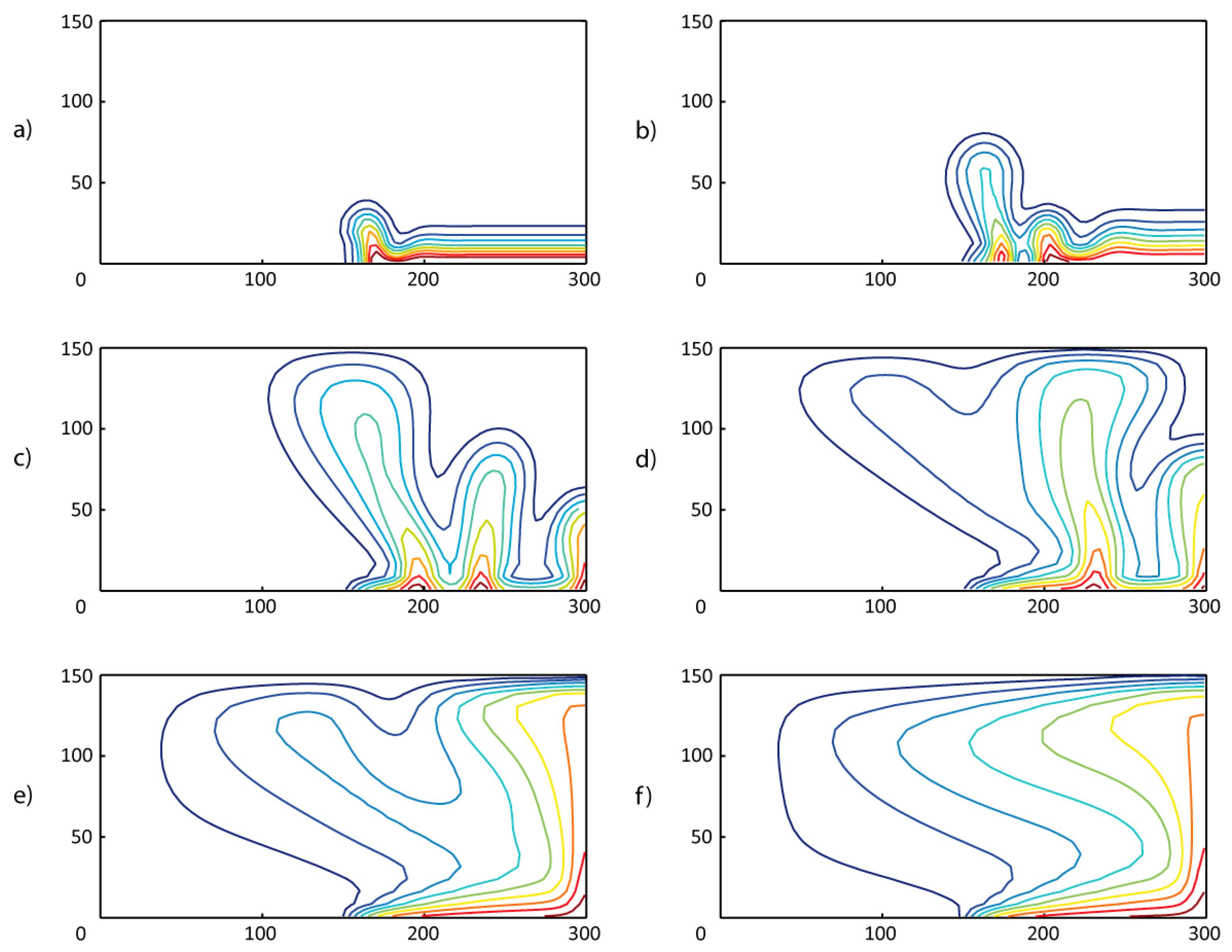
Finally, to demonstrate the reliability and robustness of the network model, Figure 9 shows the evolution of temperature patterns from transient to steady-state. The results obtained are very similar to those provided by Elder in its original work.

5. Comments and Conclusions

The network method applied to fluid flow and heat transport in porous media is seen to provide feasible solutions to standard benchmark problems. The widespread use of the new versions of PSPICE, the code used for the simulation, reflects its applicability to a large variety of problems. The programming rules for the network design are very few since only three or four electrical devices are used, regardless of the kind of non-linearity and coupling existing in the governing equations and of the type of boundary conditions. Another advantage of the proposed method is that the user requires no mathematical manipulations other than the programming routines required for data treatment to carry out the interpolation and graphical representation of the results. Of course, the programmer must have a basic knowledge of the foundations of circuit theory.

Starting from the coupled finite differences–differences (space) differential equations (time) that arise from the mathematical model (PDEs), the design of the model follows formal steps. Each one of the two networks (one for each equation) contains a number of branches (as many as there are terms in the equations) with electrical devices, whose constitutive equations, once the equivalence between dependent variables has been established, are the equations of the term. Linear terms are implemented by simple resistors, while the rest of the terms (non-lineal or coupled terms, and boundary conditions) are implemented by controlled sources specified by the software; consequently, only two kinds of electrical device are required, reducing the design to a very few rules. The rest of the work (the coupling of the adjacent network cells and the numerical calculus) is made by the code of simulation.

The benchmark type geothermal–hydrological problems proposed to test the suitability of the network method provide reliable results both qualitatively and quantitatively. This allows its application to real 2-D cases with non-homogeneous and anisotropic media subjected to any kind of boundary condition. In the slender box application, the simulations provide the Rayleigh dependence on the steady state patterns for a wide range of the physical parameters, and comparisons with other standard numerical solutions produce deviations that may be considered acceptable within the civil engineering field. In addition, sensitivity analysis as regards the mesh grid leads to the conclusion that small grids of the order of 400 cells (20 × 20) are sufficiently to provide reliable solutions with relatively small computing times. In the horizontal plates heated from below, or the Elder problem, the method again provides precise solutions for a wide range of parameter values that define the Rayleigh number of this problem. The solution patterns represent the marked asymmetry of the temperature and streamfunction distributions in the domain, and their quantitative comparisons with numerical solution of Elder (close to that of his experiments) produce deviations that can be considered acceptable. In light of the above, the proposed method is a good numerical tool for basic and real studies related with geothermal–hydrological problems.

References

- Cheng, P. Heat transfer in geothermal systems. Adv. Heat Transf. 1978, 14, 1–105. [Google Scholar]
- Revil, A.; Schwaeger, H.; Cathles, L.M.; Manhardt, P.D. Streaming potential in porous media: 2. Theory and application to geothermal systems. J. Geophys. Res. Solid Earth 1999, 104, 20033–20048. [Google Scholar] [CrossRef]
- Pruess, K. Enhanced geothermal systems (EGS) using CO2 as working fluid—A novel approach for generating renewable energy with simultaneous sequestration of carbon. Geothermics 2006, 35, 351–367. [Google Scholar] [CrossRef]
- Ciriello, V.; Bottarelli, M.; Di Federico, V.; Tartakovsky, D.M. Temperature fields induced by geothermal devices. Energy 2015, 93, 1896–1903. [Google Scholar] [CrossRef]
- Böttcher, N.; Watanabe, N.; Görke, U.J.; Kolditz, O. Geoenergy Modeling I: Geothermal Processes in Fractured Porous Media; Springer: Berlin, Germany, 2016. [Google Scholar]
- Liu, Z.; Yao, Y.; Wu, H. Numerical modeling for solid–liquid phase change phenomena in porous media: Shell-and-tube type latent heat thermal energy storage. Appl. Energy 2013, 112, 1222–1232. [Google Scholar] [CrossRef]
- Adler, P. Porous Media: Geometry and Transports; Elsevier: Amsterdam, The Netherlands, 2013. [Google Scholar]
- Horton, C.W.; Rogers, F.T. Convection currents in a porous medium. J. Appl. Phys. 1945, 16, 367–370. [Google Scholar] [CrossRef]
- Lapwood, E.R. Convection of a fluid in a porous medium. Math. Proc. Camb. Philos. Soc. 1948, 44, 508–521. [Google Scholar] [CrossRef]
- Wooding, R.A. Steady state free thermal convection of liquid in a saturated permeable medium. J. Fluid Mech. 1957, 2, 273–285. [Google Scholar] [CrossRef]
- Elder, J.W. Steady free convection in a porous medium heated from below. J. Fluid Mech. 1967, 27, 29–48. [Google Scholar] [CrossRef]
- Elder, J.W. Transient convection in a porous medium. J. Fluid Mech. 1967, 27, 69–96. [Google Scholar] [CrossRef]
- Holzbecher, E. Modelling Density-Driven Flow in Porous Media; Springer: Berlin, Germany, 1998. [Google Scholar]
- Vafai, K. Handbook of Porous Media; CRC Press: Boca Raton, FL, USA, 2015. [Google Scholar]
- Diersch, H.J.; Kolditz, O. Variable-density flow and transport in porous media: Approaches and challenges. Adv. Water Resour. 2002, 25, 899–944. [Google Scholar] [CrossRef]
- Bejan, A.; Mamut, E.; Pop, I. Emerging Technologies and Techniques in Porous Media; Springer-Verlag New York Inc.: New York, NY, USA, 2004. [Google Scholar]
- Nield, D.A.; Bejan, A. Convection in Porous Media, 5th ed.; Springer: New York, NY, USA, 2017. [Google Scholar]
- Straus, J.M. Large amplitude convection in porous media. J. Fluid Mech. 1974, 64, 51–63. [Google Scholar] [CrossRef]
- Hickox, C.E.; Gartling, D.K. A numerical study of natural convection in a horizontal porous layer subjected to an end-to-end temperature difference. J. Heat Trans. 1981, 103, 797–802. [Google Scholar] [CrossRef]
- Debéda, V.; Catiagirone, J.P.; Watremez, P. Local multigrid refinement method for natural convection in fissured porous media. Numer. Heat Transf. B Fundam. 1995, 28, 455–467. [Google Scholar] [CrossRef]
- Šarler, B.; Perko, J.; Chen, C.S. Radial basis function collocation method solution of natural convection in porous media. Int. J. Numer. Methods Heat Fluid Flow 2004, 14, 187–212. [Google Scholar] [CrossRef]
- Morales, J.L.; Moreno, J. A.; Alhama, F. Application of the network method to simulate elastostatic problems defined by potential functions. Applications to axisymmetrical hollow bodies. Int. J. Comput. Math. 2012, 89, 1781–1793. [Google Scholar] [CrossRef]
- Caravaca, M.; Sanchez-Andrada, P.; Soto, A.; Alajarin, M. The network simulation method: A useful tool for locating the kinetic-thermodynamic switching point in complex kinetic schemes. Phys. Chem. Chem. Phys. 2014, 16, 25409–25420. [Google Scholar] [CrossRef] [PubMed]
- Sánchez Pérez, J.F.; Moreno, J.A.; Alhama, F. Numerical simulation of high-temperature oxidation of lubricants using the network method. Chem. Eng. Commun. 2015, 202, 982–991. [Google Scholar] [CrossRef]
- Marín, F.; Alhama, F.; Meroño, P.A.; Moreno, J.A. Modelling of stick-slip behaviour in a Girling brake using network simulation method. Nonlinear Dyn. 2016, 84, 153–162. [Google Scholar] [CrossRef]
- Soto-Meca, A.; Alhama, F.; González-Fernández, C. Density-driven flow and solute transport problems. A 2-D numerical model based on the network simulation method. Comput. Phys. Commun 2007, 177, 720–728. [Google Scholar] [CrossRef]
- PSPICE 6.0, Microsim Corporation Fairbanks: Irvine, CA, USA, 1994.
- González-Fernández, C.F.; Alhama, F. Heat transfer and the network simulation method. In Network Simulation Method; Horno, J., Ed.; Research Signpost: Trivandrum, India, 2001. [Google Scholar]
- MATLAB and Statistics Toolbox Release 2012b, MathWorks, Inc.: Natick, MA, USA, 2012.
- Bénard, H. Les tourbillions cellulaires dans mappe liquid transportant de la chaleur par convections en regime permanent. Rev. Gen. Sci. Pures Appl. Bull. Assoc. 1900, 11, 1261–12712, 1309–1328. [Google Scholar]
- Elder, J.W.; Simmons, C.T.; Diersch, H.-J.; Frolkovič, P.; Holzbecher, E.; Johannsen, K. The Elder Problem. Fluids 2017, 2. [Google Scholar] [CrossRef]
Figure 1.
Physical scheme and geometry: (a) slender vertical box; and (b) Elder problem.
Figure 2.
Nomenclature and network model: (a) streamfunction variable; and (b) temperature.
Figure 3.
Steady state temperature pattern for the first application (Ra = 200): (a) Case 1; (b) Case 2; and (c) Case 3.
Figure 4.
Steady state streamfunction patterns for the first application (Ra = 200): (a) Case 1; (b) Case 2; and (c) Case 3.
Figure 5.
Comparison between network method and finite-difference technique: (a) Ra = 200; (b) Ra = 300; and (c) Ra = 400.
Figure 6.
Sensitivity analysis for different grid sizes: (a) Ra = 200; (b) Ra = 300; and (c) Ra = 400 (―: (20 × 80);⋯⋯: (20 × 50); - - -: (20 × 80)).
Figure 7.
Steady state temperature patterns for the Elder problem: (a) case 1; and (b) case 2.
Figure 8.
Steady state streamfunction patterns for the Elder problem: (a) case 1; and (b) case 2.
Figure 9.
Evolution of transient to steady state temperature patterns for the Elder problem from the initial conditions (a) to the steady-state (f).