User-Aware Electricity Price Optimization for the Competitive Market ^†

Abstract

Demand response mechanisms and load control in the electricity market represent an important area of research at the international level: the trend towards competition and market liberalization has led to the development of methodologies and tools to support energy providers. Demand side management helps energy suppliers to reduce the peak demand and remodel load profiles. This work is intended to support energy suppliers and policy makers in developing strategies to act on the behavior of energy consumers, with the aim to make a more efficient use of energy. We develop a non-linear optimization model for the dynamics of the electricity market, which can be used to obtain tariff recommendations or for setting the goals of a sensibilization campaign. The model comes in two variants: a stochastic version, designed for residential electricity consumption, and a deterministic version, suitable for large electricity users (e.g., public buildings, industrial users). We have tested our model on data from the Italian energy market and performed an extensive analysis of different scenarios. We also tested the optimization model in a real setting in the context of the FP7 DAREED project (http://www.dareed.eu/), where the model has been employed to provide tariff recommendations or to help the identification of goals for local policies.

1. Introduction

One of the main research objectives in the field of the efficient use of electric energy is the design and experimentation of new mechanisms to lower the electricity consumption and to improve the electricity consumption via demand shifting. Increasing energy efficiency requires a reduction of energy demand peaks by shifting part of the energy consumption in off-peak hours. This can be done via demand response (DR) mechanisms and load control. Beside environmental advantages, DR mechanisms can also lead to economic gains. In particular, they provide end-users with the opportunity to reduce their electricity costs by responding to market prices.

We developed a non-linear optimization model to provide support for political and economic decision makers to define new business models. In the complex and heterogeneous context of the electricity market, our work aims to create a comprehensive model, which collects all of the main variables and parameters that are relevant in the analysis of DR mechanisms for sustainable energy tariffs. Our model components are: (1) elasticity model for customer behavior (i.e., an elastic model to characterize the demand-response behavior and load management), (2) Time of Use (ToU) DR mechanisms, (3) user perception of energy consumption (i.e., a model for the relationship between real and perceived user consumption) and (4) risk aversion behavior of customers. Our aim is to present a new conceptual approach to model the recently deregulated power markets. Differently from previous literature, our approach works on a time scale of one year. It is focused on ToU-based prices, but it also takes into account many factors that are crucial for modeling a realistic market and that are not considered by existing price optimization approaches (e.g., multiple customers and cognitive aspects, multiple tariffs). By simulating the behavior of the key actors in the electricity market, our model can identify equilibrium situations in which each involved part can pursue its own goals and yet bring the system to a situation of global benefit. To the best of our knowledge, there is no well-established model for the definition of electricity tariffs via optimization and definitely no other model that takes into account existing tariffs and cognitive user aspects.

In our experimental results, we assess what the effect of changing model parameters would be by testing the model in different scenarios. In particular, we show that no model equilibrium (i.e., benefits for both energy provider and customers) is possible in the Italian electricity market under realistic assignments of all of the model parameters. Differently from previous works, which only consider customer elasticity and load consumption, we also show in our results that perception accuracy can significantly affect the demand response model. Our model can be employed in different settings: (1) by an energy utility to obtain tariff recommendations, (2) to obtain recommendations about changes in the customer behavior parameters (e.g., customer flexibility, perception accuracy) and (3) by policy makers to shape incentive mechanisms and to define policy goals. The case study has been defined by merging statistical census, population information and data from the national energy market manager in accordance with the different parameters of our model. We also tested the optimization model in a real setting in the context of the FP7 DAREED project: namely, our optimization model has been employed by staff at ENEL (the main energy provider in Italy) to support the design of attractive tariffs for an Italian town.

The paper is organized as follows. Section 2 provides an analysis of the current state of the art on demand response mechanisms, showing the innovative aspects and the focus of this work. Section 3 describes the proposed optimization model (which comes in a stochastic and a deterministic variant), which take into account the behavior of multiple customers and energy providers. Section 4 presents how our model has been applied to the Italian energy market, and it provides the results and discussion of market scenarios and real-life tests. Concluding remarks follow in Section 5.

2. Related Work

In this section, we introduce some useful notions in demand response programs with a focus on the price-based DR mechanisms used in our work. Demand response programs studied in the literature can be divided into two main groups: price-based and incentive-based mechanisms. In this paper, we modeled the electricity market using price-based demand response, which is related to the changes in energy consumption by customers in response to the variations of their purchase prices. This group includes DR mechanisms like Time of Use (ToU) pricing, real-time pricing and critical-peak pricing rates. If the price varies significantly, customers can respond to the price structure with changes in their pattern of energy use. We focus on ToU mechanisms, which define different prices for electricity usage during different periods: the tariffs reflect the average cost of generating and delivering power during those periods. A more detailed overview of demand response schemes can be found in [1,2,3].

For its composition, our model and its different parameters can be adjusted to match the market of different countries, regulations and market scenarios. The approaches from the literature in this field are very heterogeneous and difficult to compare directly, so our aim is to present the works that are related to each part of our approach, so as to underline that, differently from previous literature, we grouped all components in a single and holistic model of the electricity market. In the rest of this section, we split the presentation according to the different components of the model.

2.1. Benefits of Time of Use Mechanisms for Users

The most widespread DR mechanism in practice is given by ToU-based tariffs. Usually, in this mechanism, peak periods have higher prices than off-peak periods [4]. Concerning the study of ToU mechanisms and load management for users, [5] shows an optimal load management strategy for residential consumers, and [6] studies how users can adjust their load level according to a specific DR program.

Our paper is focused on ToU-based tariffs applied to a set of residential and large public customers. However, unlike [5,7], here we are more concerned with defining ToU prices, rather than how to optimally take advantage of them. We therefore use a simpler model for the customer behavior, related to the works that will be discussed in Section 2.2. This choice allows us to obtain an approximate model for a large electricity market (the Italian one, in our experimentation).

2.2. Optimization Approaches to Model Electricity Market Prices

It is possible, in the current state of the art, to identify three major trends to model the electricity market: optimization models, equilibrium models and simulation models. A survey of the literature on electricity market models can be found in [8]. We used optimization models for the definition of energy prices and provider tariffs: a survey on demand response pricing methods and optimization algorithms is presented in [9]. Optimization approaches to define dynamic prices have been proposed in [10,11,12,13]. All such works focus on the definition of day-ahead prices for a period of 24 h and for a single customer (or a single group of homogeneous customers).

A model of an energy service provider in the electricity market is defined in [14]. This model results in an optimization problem for calculating the optimal electric power and energy selling prices that maximize the economic profits obtained by the provider. Our approach works on a much coarser time scale (one year). It is focused only on ToU-based prices, but our emphasis is on modeling reasonably well the actors and their behavior for the definition of electricity tariffs via optimization by taking into account existing tariffs and cognitive aspects.

2.3. Elastic Model for User Consumption

After the electricity market liberalization, consumers have more opportunities to reduce their electricity costs by choosing the proper tariff and modifying their load profile. Therefore, modeling how the electricity demand shifts is a necessary step to obtain an optimization model for the electricity market. The work in [15] proposes an elastic model to characterize the demand-response behavior and load management, and it describes how the consumers’ behavior can be modeled using a matrix of self- and cross-elasticity. The same elastic demand-response model is employed in [10,11], which take into account also other incentive schemes.

Some work in the literature, while not proposing models for demand shifting, analyze some of the main features. The work in [16] assesses the impacts of ToU tariffs on a dataset of residential users from the Province of Trento in Northern Italy in terms of changes in electricity demand, price savings, peak load shifting and peak electricity demand at sub-station level, but the paper provides no mathematical model. In general, the response of the customers to the DR programs affects the daily load curve. Therefore, the load duration curve may change considerably due to the responsiveness of the customers over a year [17]. For this reason, the effects of DR need to be investigated for a longer time horizon than the daily one. In our paper, we employ a modified version of the elastic demand-response model from [15], which has been adapted to ToU-based prices over a yearly time horizon. This is a major difference w.r.t. the existing literature: it is better suited for the task of defining new tariffs, and it allows us to better identify trends and assess how the characteristics of the market and the customers affect the annual consumption profiles.

2.4. Perception of the Electricity Consumption

Consumption and cost awareness have an important role for the effectiveness of demand response schemes. However, many customers do not understand how to lower electricity costs and call for a device that displays the current power output [18], and consumer behavior is complex and difficult to represent in traditional economic theories of decision-making [19]. The work in [20] shows how real-time price elasticity provides important information on the demand response of consumers and provides a quantification of the real-time relationship between total peak demand and spot market prices by finding a low real-time price elasticity. The works in [21,22] study how customers respond to price changes and which price indicators are more relevant in this respect to guide the demand shift. The authors of [21] try also to account for misperception of energy consumption, which is further analyzed in [23]. The latter work in particular attempts to design a model for the relationship between real and perceived consumption via regression techniques (i.e., function fitting). The paper proposes a (scale dependent) model in logarithmic scale and concludes that customers tend to slightly overestimate low-energy activities and significantly underestimate activities with high energy consumption.

In our work, we take into account the effect of perception accuracy in the consumer behavior using an analytical model. We do not employ the function proposed in [23] due to its dependence on scale: instead, we try to obtain a similar curve by using a different function, discussed in Section 3. We insert this perception model into a richer and more complex model that already takes into account demand elasticity and ToU-based prices.

2.5. Multiple Users, Competitive Market and Risk Aversion

All works cited in Section 2.2 focus on the definition of a single customer or a single group of homogeneous customers to model the electricity market. In our work, we model multiple groups of homogeneous customers, and we aim to show how multiple, different consumers react to electricity prices. Differently from the existing literature, we model multiple tariffs in order to represent different competitors in the recently deregulated electricity market. Our aim is to present, with our work, a new conceptual approach to model the recently deregulated power markets (Figure 1). The interaction of competitive agents in the electricity market is usually modeled through equilibrium problems that ensure profit maximization for all of the agents. For example, [24] models the competitive behavior of the electric energy generation market by incorporating a set of constraints, namely the equilibrium constraints, into a traditional production cost model. Usually, consumer choices are marked by personal proclivities, risk aversion and misperception of their consumption, as shown in [25]. Therefore, our model analyzes a market situation where the users exhibit risk aversion, which is natural in this type of market. The user risk aversion gives rise to an interesting economical interpretation of our model.

3. Modeling Approach and Formulation

Each model component is presented here separately. The most natural application of our model is the computation of ToU price recommendation for new tariffs of an energy provider in the situation of a competitive market. In particular, our model is developed from the point of view of a single energy provider whose tariffs are represented as decision variables in our model. The fixed and non-modifiable tariffs are those of competitor providers represented in our model. Moreover, we have developed two distinct modeling approaches for the way customers can switch to a new tariff: the two approaches are presented in the introduction to Section 3.2.

3.1. Set of Tariffs

We consider a set T of ToU-based tariffs ${\tau }_i$, defined over a common price band scheme. The scheme specifies a set P of pre-defined price bands ${\pi }_j$: the exact configuration (e.g., start, end) of each price band is left unspecified, but we assume that for each band ${\pi }_j$, the total number of hours $|{\pi }_j|$ over a period of one year is available.

Each ToU-based tariff is defined by a price value $p_{i,j}$ for each band. We assume that a subset $T_f$ of the tariffs is fixed, i.e., it cannot be altered by the energy provider. For each ${\tau }_i\in T_f$, the prices are constant values. The remaining tariffs are variable, and their prices are the main decision variables in our model. We assume that the prices take values over a bounded range, i.e., $p_{i,j}\in [{\underline{p}}_{i,j},{\overline{p}}_{i,j}]$. As long as the bounds are large enough, this assumption is sufficiently general to handle practical scenarios. Finally, we assume that a subset $T_o$ of tariffs is owned by the energy provider, i.e., the provider earns profit (and pays the cost) for the electricity consumed under such tariffs.

This setup is sufficient to handle a number of interesting cases. Variable tariffs are those for which we wish to obtain price recommendations. Tariffs that are both fixed and owned represent pre-existing contracts that cannot be altered. Tariffs that are fixed and not owned are those offered by competitor providers. The point of view is that of a single energy provider that obtains tariff recommendations.

3.2. Customer Tariff Choice

The model comes in two variants for customers representation and tariff choice. For the first case, we take into account the behavior of a set C of homogeneous groups of customers, often referred to as “customer classes”. We model the tariff switching as a stochastic process as detailed in the next Section 3.2.1. For the second case (i.e., a group of large customers), the model could be used to support the definition of tailored tariffs for public buildings or industrial customers: in this case, the effect of demand shifts on the wholesale price should be disregarded, and finally, the tariff choice should be deterministic rather than stochastic. This deterministic choice behavior could be modeled by formulating the Karush–Kuhn–Tucker (KKT) optimality conditions for a tariff selection subproblem. This modeling is shown in Section 3.7.

3.2.1. Stochastic Tariff Selection for Residential Customers

We take into account the behavior of a set C of customer classes. Each customer class ${\kappa }_k\in C$ is associated with an original tariff $\tau \left({\kappa }_k\right)$, which must be fixed (i.e., $\tau \left({\kappa }_k\right)\in T_f$). Moreover, we assume that the approximate number of customers in each class (let this be $|{\kappa }_k|$) is known.

Customers may switch to a new tariff, based on its economic benefits. In particular, we assume that each customer in a group can switch tariff with a probability that depends on the obtained savings. Formally, let $c_{k,i}$ be the electricity cost for customer class ${\kappa }_k$ under tariff ${\tau }_i$. The $c_{k,i}$ term is a constant if ${\tau }_i$ is fixed, and a decision variable if ${\tau }_i$ is variable: the computation of such cost values will be discussed in the forthcoming Section 3.3. Technically, we say that the customers are likely to exhibit a certain degree of risk aversion, so the savings for class ${\kappa }_k$ under tariff ${\tau }_i$ are given by:

$$\begin{array}{c}\hfill s_{k,i}=\left\{\begin{array}{cc}{\rho }_k{c}_{k,\tau \left({\kappa }_k\right)}\hfill & \mathrm{if}{\tau }_i=\tau \left({\kappa }_k\right)\hfill \\ max(0,c_{k,\tau \left({\kappa }_k\right)}-c_{k,i})\hfill & \mathrm{otherwise}\hfill \end{array}\right.\end{array}$$

(1)

where $0<{\rho }_k<1$ is a risk aversion coefficient. In practice, staying with the current tariffs is considered equivalent to saving a factor ${\rho }_k$ of the current cost: this provides an intuitive approach to define the value of ${\rho }_k$ based on questionnaires or existing data.

As we mentioned, we model the tariff switching as a stochastic process. In particular, we assume that all tariff choices for a given customer class are independent and identically distributed. Formally, we introduce a set of stochastic binary variables $Y_{k,i}$ that are equal to one if a customer in class ${\kappa }_k$ adopts tariff ${\tau }_i$:

$$\begin{array}{c}P(Y_{k,i}=1)=\frac{s_{k,i}}{{\sum }_{{\tau }_i\in T}{s}_{k,i}}\hfill \end{array}$$

(2)

i.e., the probability is proportional to the savings computed with Equation (1). The number of customers of class ${\kappa }_k$ that adopt tariff ${\tau }_i$ can be obtained by summing $Y_{k,i}$ for $|{\kappa }_k|$ times. The expected value of this expression is given by:

$$\begin{array}{c}\hfill E\left[\sum _{k=0}^{|{\kappa }_k|-1}{Y}_{k,i}\right]=|{\kappa }_k|E[Y_{k,i}]=|{\kappa }_k|\frac{s_{k,i}}{{\sum }_{{\tau }_i\in T}{s}_{k,i}}\end{array}$$

(3)

Therefore, on average, the customers in each class spread over the available tariffs proportionally to the value of $s_{k,i}$. We use this information to define the tariff selection (and risk aversion) component of our model, which is given by:

$$\begin{array}{cc}{y}_{k,i}=\frac{s_{k,i}}{{\sum }_{{\tau }_i\in T}{s}_{k,i}}\hfill & \hfill \forall {\kappa }_k\in C,{\tau }_i\in T\end{array}$$

(4)

$$\begin{array}{cc}{s}_{k,i}=\left\{\begin{array}{cc}{\rho }_k{c}_{k,\tau \left({\kappa }_k\right)}\hfill & \mathrm{if}{\tau }_i=\tau \left({\kappa }_k\right)\hfill \\ max(0,c_{k,\tau \left({\kappa }_k\right)}-c_{k,i})\hfill & \mathrm{otherwise}\hfill \end{array}\right.\hfill & \hfill \forall {\kappa }_k\in C,{\tau }_i\in T\end{array}$$

(5)

$$\begin{array}{cc}{y}_{k,i}\in [0,1]\hfill & \hfill \forall {\kappa }_k\in C,{\tau }_i\in T\end{array}$$

(6)

$$\begin{array}{cc}{c}_{k,i}\in {\mathbb{R}}^{+}\hfill & \hfill \forall {\kappa }_k\in C,{\tau }_i\in T\end{array}$$

(7)

The $y_{k,i}$ variables represent the fraction of customers of class ${\kappa }_k$ that adopt tariff ${\tau }_i$. Due to the presence of “max” operators in Equation (1), this model component is non-smooth (piecewise linear in particular). The “max” operators can be linearized by using special ordered sets of type 2, which require the addition of binary variables. In our experimentation, however, we employ the modeling system GAMS (See http://www.gams.com/) and let the software take care of the linearization.

3.3. Energy Demand and Perception Accuracy

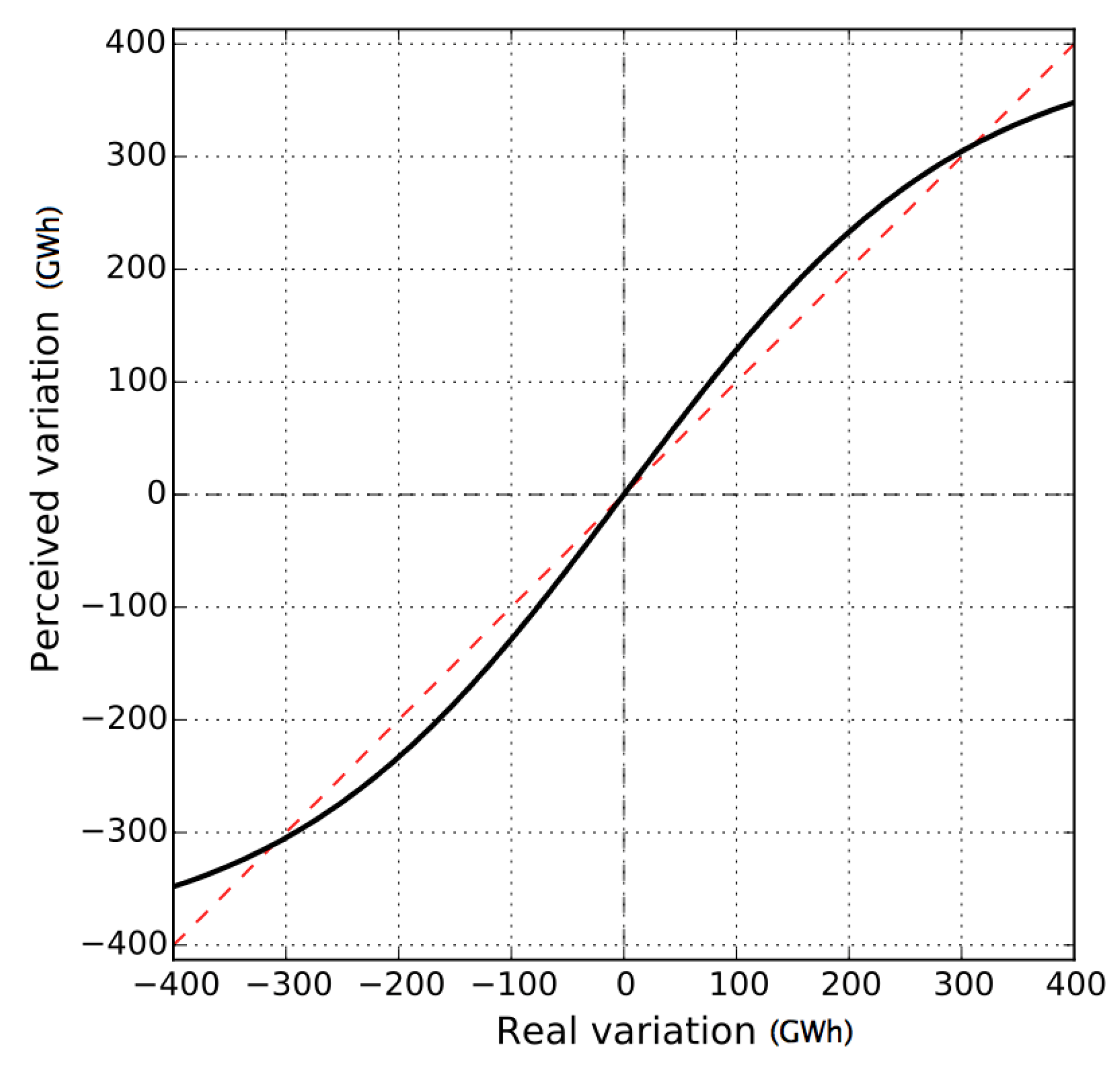
In this paper, we take into account the perception accuracy in the demand response behavior. The main idea is to view the ${\tilde{d}}_j^{(k,i)}$ variables that will be introduced in Section 3.4 as perceived variations. We then introduce a second set of variables ${\tilde{r}}_j^{(k,i)}$ to represent the corresponding real variations. The two sets of variables are related by a custom model based on results from [23]. In particular, our model is based on a sigmoid function in the form:

$$\begin{array}{c}\hfill y=sig(x,\alpha ,{\beta }_{\kappa })=\alpha \left(\frac{2}{1+e^{-2\frac{1}{\alpha {\beta }_k}x}}-1\right)\end{array}$$

(8)

The $\alpha$ parameter determines the scale of the sigmoid; the ${\beta }_k$ parameter controls the growth of the sigmoid, which is specific to each customer class ${\kappa }_k$. Assuming that y is a perceived variation, that x is a real variation and that ${\beta }_k>0$, then the sigmoid exhibits the qualitative behavior reported in [23]: for values close to zero, y is a overestimation of x; for values close to $\alpha$, y is an underestimation of x. The break-even point depends on the value of ${\beta }_k$. If ${\beta }_k<1$, there is a bias toward overestimation (i.e., for a wide range of values, the perceived variation is larger than the real one), if ${\beta }_k>1$, there is a bias toward underestimation (i.e., for a wide range of values, the perceived variation is smaller than the real one). Figure 2 shows this behavior in the sigmoid function for $\alpha$ = 400, ${\beta }_k$ = 0.75.

We use our sigmoid function to relate the average perceived and real variations of electrical power consumption. Those are obtained by dividing the variation variables ${\tilde{d}}_j^{(k,i)}$ and ${\tilde{r}}_j^{(k,i)}$ (which represent energy values) by the total number of hours in the price bands. Therefore, we obtain:

$$\begin{array}{c}\hfill \frac{1}{|{\pi }_j|}{\tilde{d}}_j^{(k,i)}=sig\left(\frac{1}{|{\pi }_j|}{\tilde{r}}_j^{(k,i)},\alpha ,{\beta }_k\right)\end{array}$$

(9)

We can then use the real variation variable to compute the total electricity demand for each individual customer of class ${\kappa }_k$, in each price band and for each tariff. Formally, we have:

$$\begin{array}{c}\hfill d_j^{(k,i)}={\widehat{dr}}_j^{(k,i)}+{\tilde{r}}_j^{(k,i)}\end{array}$$

(10)

where the $d_j^{(k,i)}$ represents the total demand. For the original tariff, i.e., ${\tau }_i=\tau \left({\kappa }_k\right)$, the total demand will be the same as the original real demand, i.e., $d_j^{(k,i)}={\widehat{dr}}_j^{(k,i)}$. The demand variables $d_j^{(k,i)}$ can be used to compute the cost of energy for each individual customer under each tariff, i.e., the value of the $c_{k,i}$ variables from Section 3.2. This is given by:

$$\begin{array}{c}\hfill c_{k,i}=\sum _{{\pi }_j\in P}{p}_{i,j}{d}_j^{(k,i)}\end{array}$$

(11)

3.4. Demand Response Behavior

We assume that customers can shift their consumption depending on the energy prices, i.e., they are capable of a demand response behavior. Many demand response programs (including ToU-based prices) have been considered in the literature, but only a few mathematical models have been provided. We have developed a variant of one of the most widely-employed approaches, which was proposed in [15] and is based on a cross-elasticity matrix. Essentially, the approach uses a linear transformation to map the variation of prices to variations of demand:

$$\begin{array}{c}\hfill \tilde{d}=ϵ\tilde{p}\end{array}$$

(12)

where $\tilde{d}$ is a vector of demand variations over multiple time periods, $\tilde{p}$ is a vector of (normalized) price variations and $ϵ$ is called the cross-elasticity matrix. The original approach by [15] and employed in [10,11,26] is designed for time periods of homogeneous duration and day-ahead prices.

We adapted the model to ToU-based tariffs with price bands of non-uniform duration, over a year-long time period. The main idea is simply to introduce variables to represent the variation in the yearly electricity demand of an individual customer, for each price band ${\pi }_j$. Since we consider multiple customer classes and tariffs in our model, we need separate variables ${\tilde{d}}_j^{(k,i)}$ for each class ${\kappa }_k$ and tariff ${\tau }_i$. The demand variation is therefore connected to the tariff prices by:

$$\begin{array}{c}\hfill {\tilde{d}}_j^{(k,i)}=\sum _{{\pi }_h\in P}{\widehat{dr}}_h^{\left(k\right)}{ϵ}_{j,h}{\tilde{p}}_h^{(k,i)}\end{array}$$

(13)

where the ${\tilde{p}}_h^{(k,i)}$ variables represent normalized price variations. The term ${\widehat{dr}}_h^{\left(k\right)}$ is a problem parameter, representing the original demand for an individual customer of class ${\kappa }_k$, in price band ${\pi }_h$.

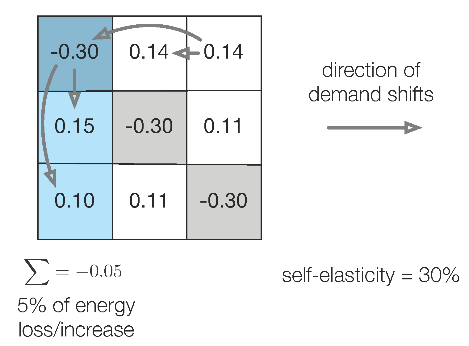
With respect to the demand for electricity, a self-elasticity coefficient relates the demand during a band period to the price during that band. A rescheduling of consumption implies that the consumer reduces its electricity demand during some bands and increases it during other (cross-elasticity matrix coefficients). In particular, the terms on the matrix diagonal are always non-positive and are called self-elasticity coefficients. The other terms are always non-negative. Intuitively, the self-elasticity coefficients describe how the demand within each band depends on the prices. The other terms in the matrix represent how the demand shifts from price bands (self-elasticity cells) and to price bands (others two bands in the same column). The sum of the coefficients on each column corresponds to the net increase/decrease of consumption when the normalized prices increase/decrease: we refer to such a quantity as the loss factor. If the loss factor is zero, changing the prices may alter the distribution of the demand between the price bands, but not its total value. Figure 3 reports an example of cross-elasticity matrix, with a visual representation of the demand flows. See [27] for further details.

For normalizing the price variations, we use the average price under the original tariff, i.e.,

$$\begin{array}{c}\hfill {\tilde{p}}_j^{(k,i)}=\frac{p_{i,j}-p_{\tau \left({\kappa }_k\right),j}}{{\sum }_{{\pi }_h\in P}{p}_{\tau \left({\kappa }_k\right),h}}\end{array}$$

(14)

Having weighted contributions by ${\widehat{dr}}_j^{\left(k\right)}$ and normalized prices provides us with a way to interpret intuitively the ${ϵ}_{j,h}$ coefficients. In particular, if the price in band ${\pi }_h$ roughly doubles (i.e., the normalized variation is one), then:

• The demand in band ${\pi }_h$ (the same band) decreases by a factor $|{ϵ}_{h,h}|$ of the original demand (we recall that self-elasticity coefficients are non-positive).
• A factor ${ϵ}_{j,h}$ of the original demand of band ${\pi }_h$ shifts to band ${\pi }_j$.

3.5. Wholesale Energy Price

The price of the electricity on the wholesale market (i.e., the electricity cost for the provider) depends on the national energy demand, with larger demand values leading to higher prices. This allows a provider to increase profit by exploiting the demand response behavior and reducing the wholesale energy price. In ToU-based tariffs, demand shifts are obtained by lowering prices: hence, the dependency of the wholesale electricity on the demand provides opportunities for win-win situations, where both the provider and the customers obtain some gain. It is important to underline that the wholesale energy price variations along the bands are relevant only if the electricity customers demand is large. If this is not the case, the wholesale energy price for each price band can be considered as a constant parameter. We focus on the retail electricity market, and we consider a demand response problem in a market situation of multiple tariffs and consumers where every entity tries to maximize its own benefits.

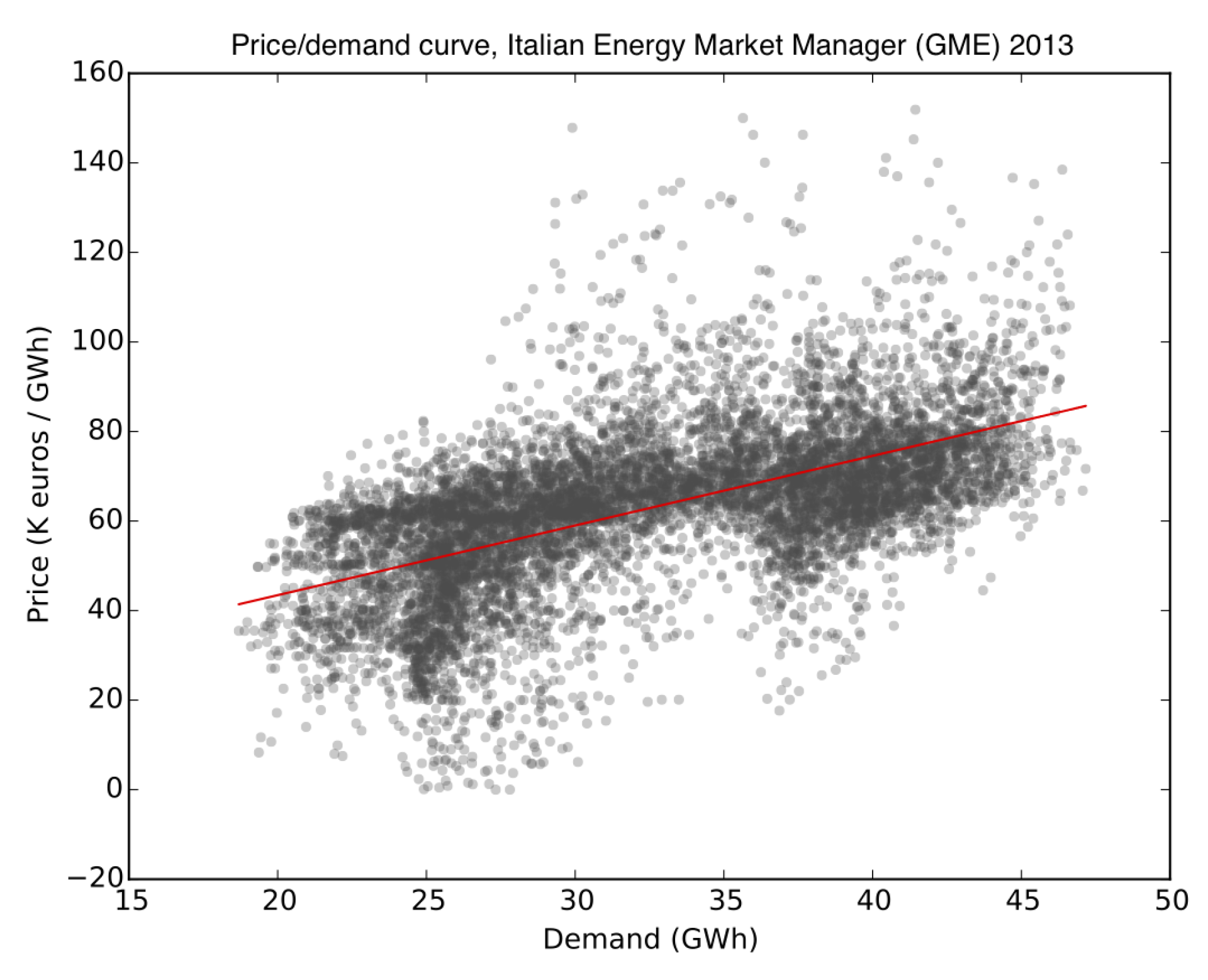
Many works (e.g., [2]) assume the wholesale price-demand curve to be super linear, based on the idea that more expensive power generators are activated when the demand is large. We have tested this conjecture for the Italian energy market, which is organized by a (government controlled) corporation called GME (Italian Energy Market Manager) , which issues a reference electricity price and keeps track of the national consumption on a hourly basis. By checking these data, we have observed a weak and linear, rather than super-linear, correlation (see Figure 4). We have therefore decided to use a linear relation to estimate the wholesale energy price $w_j$ for each band j, which consists of ($\forall {\kappa }_k\in C,{\pi }_j\in P$):

$$\begin{array}{c}{w}_j={\mu }_1\left(\sum _{{\kappa }_k\in C}demand({\kappa }_k,{\pi }_j)+b_j\right)+{\mu }_0\hfill \end{array}$$

(15)

$$\begin{array}{c}demand({\kappa }_k,{\pi }_j)=\sum _{{\tau }_i\in T}|{\kappa }_k|y_{k,i}{d}_j^{(k,i)}\hfill \end{array}$$

(16)

$$\begin{array}{l}{w}_j\in {\mathbb{R}}^{+}\end{array}$$

(17)

where $demand({\kappa }_k,{\pi }_j)$ is the total demand of the customers of class ${\kappa }_k$ in price band ${\pi }_j$, and it is given by the product $|{\kappa }_k|y_{k,i}$, which is the number of customers of class ${\kappa }_k$ that adopt tariff ${\tau }_i$. The $b_j$ term in Equation (15) represents a baseline consumption, which cannot be altered by adjusting the variable tariffs. The ${\mu }_1$ and ${\mu }_0$ terms are the coefficients of the linear relation.

3.6. Provider Profit and Problem Objective

The most natural problem objective for designing a new tariff is to maximize the provider profit. This is also the natural problem objective if we want to employ our model just to estimate/simulate the behavior of a provider in a given market configuration. In detail, the objective function of our models is:

$$\begin{array}{c}\hfill maxz=\sum _{{\kappa }_k\in C}\sum _{{\pi }_j\in P}\mathit{profit}({\kappa }_k,{\pi }_j)\end{array}$$

(18)

i.e., the sum of the profit for each customer class and price band, with:

$$\begin{array}{c}\hfill \mathit{profit}({\kappa }_k,{\pi }_j)=\sum _{{\tau }_i\in T_o}|{\kappa }_k|y_{k,i}(p_{i,j}-w_j-o_j)d_j^{(k,i)}\end{array}$$

(19)

where $p_{i,j}$ is the tariff price for tariff ${\tau }_i$ and $w_j$ is the wholesale energy price. The $o_j$ term represents an overhead value, which captures indirect costs due to, e.g., energy distribution services or taxes: this is often a very significant part of the energy costs. The summation in Equation (19) is performed only on the tariffs owned by the provider.

3.7. Deterministic Model

The second variant of our model is a deterministic model for customers; representation and tariff choice: the model could be used to support the definition of tailored tariffs for public buildings or industrial customers. For the deterministic model, we calibrate different coefficients of elasticity and risk-aversion. Since our model consists of components, in this case, we simply disable the consumer perception accuracy component calibrated for residential users.

This deterministic tariff choice behavior could be modeled by formulating the KKT optimality conditions for a tariff selection subproblem. The greatest difficulty of a multi-tariff model is to correctly model user behavior. In fact, users choose their own tariff in order to minimize their energy costs, i.e., by solving an optimization problem whose objective function is in conflict with that of the energy provider. In this work, we modeled the user behavior by converting such an optimization problem into a constraint satisfaction problem by using the first-order necessary conditions that characterize the local minima, known as Karush–Kuhn–Tucker conditions.

3.7.1. Karush–Kuhn–Tucker Conditions

In the following subsection, we cast the tariff selection problem as a constraint satisfaction problem by means of the KKT conditions. See for instance [28] for details on KKT. The user tariff choice subproblem can be modeled for a single user ${\kappa }_k$ in the following way: we have variables $y_i$ that are one if tariff i is chosen and zero otherwise.

$$\begin{array}{c}minz=\sum _i{y}_i{c}_{k,i}\hfill \end{array}$$

(20)

$$\begin{array}{c}\sum _i{y}_i=1\hfill \\ y_i\in \{0,1\}\hfill & \hfill \forall {\tau }_i\in T\end{array}$$

(21)

Constraints (21) impose the choice of a single tariff for each user; the $y_i$ of Constraints (22) are all positive binary variables; and the objective function (20) considers the choice of users based on the tariff with lower overall cost.

This is an Integer Linear Programming (ILP) problem that models the choice of users tariff. Our aim is to use the KKT conditions to characterize the optimal solution to this problem. This approach requires the objective function and the constraints to be convex, so that the KKT conditions are both necessary and sufficient. ILP problems are not convex in general, which poses in principle a difficulty.

Luckily, in our case, it is possible to replace the original ILP problem with its LP (Linear Programming) relaxation: in fact, we can prove that the optimal LP solution is integer (in non-degenerate cases), and therefore equal to the optimal ILP solution. A proof of this result is provided in Appendix A.

3.7.2. Application of KKT Conditions to Our Model

As shown in the previous subsection, the KKT conditions represent necessary conditions to obtain a local optimum. Since LP problems are convex, the conditions become also sufficient to define a global optimum: hence, a problem solution exists, and it is optimal iff there are multipliers that satisfy the KKT conditions.

Now, ${\mu }_i$ is the multiplier associated with constraints $y_i\ge 0$, and $\nu$ is the multiplier associated with equality constraints; with these notations and with the Lagrangian function of the problem (${\mu }_i\ge 0,\nu \in \mathbb{R}$), the KKT conditions state that, if there exist $y_i$, ${\mu }_i$ and $\nu$ values such that:

$$\begin{array}{cc}{c}_{k,i}+\nu -{\mu }_i=0\hfill & \forall {\kappa }_k\in C,{\tau }_i\in T\hfill \end{array}$$

(22)

$$\begin{array}{cc}\sum _i{y}_i=1\hfill & \end{array}$$

(23)

$$\begin{array}{cc}{\mu }_i(-y_i)=0\hfill & \forall {\tau }_i\in T\hfill \end{array}$$

(24)

$$\begin{array}{cc}{y}_i\ge 0\hfill & \forall {\tau }_i\in T\hfill \end{array}$$

(25)

$$\begin{array}{cc}{\mu }_i\ge 0\hfill & \forall {\tau }_i\in T\hfill \end{array}$$

(26)

$$\begin{array}{cc}\nu \in \mathbb{R}\hfill & \end{array}$$

(27)

then the assignment of $y_i$ is an optimal solution for the original problem. It is possible to rewrite these conditions by eliminating ${\mu }_i$, and by taking into account all of the customer classes ${\kappa }_k$, we can finally introduce the following constraints in our model:

$$\begin{array}{cc}\sum _i{y}_{k,i}=1\hfill & \forall {\kappa }_k\in C\hfill \end{array}$$

(28)

$$\begin{array}{cc}{y}_{k,i}\ge 0\hfill & \forall {\kappa }_k\in C,{\tau }_i\in T\hfill \end{array}$$

(29)

$$\begin{array}{cc}{c}_{k,i}+{\nu }_k\ge 0\hfill & \forall {\kappa }_k\in C,{\tau }_i\in T\hfill \end{array}$$

(30)

$$\begin{array}{cc}(c_{k,i}+{\nu }_k)y_{k,i}=0\hfill & \forall {\kappa }_k\in C,{\tau }_i\in T\hfill \end{array}$$

(31)

The deterministic version of the model has the same objective function of the stochastic version, which maximizes the provider profit. Both models presented above can be enriched with other constraints that model particular aspects (e.g., the DR behavior, the perception accuracy, the wholesale price), as shown in the following sections.

4. Experimental Results and Discussion

The model and its parameters can be adjusted to approximately match the market of different countries, regulations and market scenarios.

Table 1. Model parameters.

Model Parameters	Source of Data
Number of tariff bands ${\tau }_i$ ∈ T	Data from GME and energy authority (see http://www.autorita.energia.it/it/schede/C/faq-fascenondom.htm).
Price for each band ${\pi }_j$ ∈ P	Data from the main electricity companies (see https://www.enelservizioelettrico.it/it-IT/tariffe, parameter only for fixed tariffs).
Wholesale price coefficients ${\mu }_0$ and ${\mu }_1$	Data from GME (see http://www.mercatoelettrico.org/En/Default.aspx) in order to fit a correlation between hourly electricity price and consumption to derive the coefficients.
Cross-elasticity matrix coefficients ${ϵ}_{j,h}$	Based on previous literature [15] and parameters from ISTAT (available at http://dati-censimentopopolazione.istat.it). By having access to real data, it would be possible to derive more precise coefficients through empirical model learning [29].
User classification ${\kappa }_k$ ∈ C	The data to define residential user classes is based on parameters from ISTAT (family information), and it is based on data from Confcommercio for the deterministic (industrial) case.
Perception accuracy parameters $\alpha$ and ${\beta }_k$	Data from the literature [23] and from analysis of the correlation between real and perceived user demand (the sigmoid function in which $\alpha$ determines the scale of the sigmoid, and ${\beta }_k$ controls the growth of the sigmoid).
Risk aversion coefficients of customers $\rho$	The coefficients have been estimated based on data from the literature [25,30].

contains the list of all model parameters and the source of data that we used to obtain or estimate their value. The table is meant as a tool to simplify grounding the model on different scenarios and in different countries.

4.1. Case Study: Italian Electricity Market

As a case study, we have used our approach to define a model of the Italian energy market. ToU-based tariffs in Italy are defined over three standard price bands, roughly corresponding to office hours, evenings-and-Saturdays and nights-and-Sundays. The total amount of hours for the three bands is $|{\pi }_0|=2860$, $|{\pi }_1|=2132$ and $|{\pi }_2|=3768$. The coefficients for the wholesale demand-price relation have been obtained based on data from the national energy market management corporation (see http://www.mercatoelettrico.org/En/Default.aspx, GME): in particular, we have ${\mu }_1=$~1.39 K€/GWh² and ${\mu }_0=0.013$ K€/GWh.

There are no standard and well-accepted values for the risk aversion coefficients of customers. For this reason, in our model, the risk aversion coefficient $\rho$ has been estimated based on data from [25,30], and it is equal to 0.95 for all customers. For the perception model, we have $\alpha =400$ and ${\beta }_k=0.75$ for all classes: intuitively, this means that an average consumption of 400 W on a price band is considered large and that customers tend to over-estimate demand variations (i.e., the real variation is typically smaller than expected). We model the relation using a different function (i.e., sigmoid), since the approach from [23] had poor predictive performance outside of the range considered in the original experiments. However, we took care of choosing the parameters of our sigmoid function to approximate the behavior observed in [23] on real data.

The coefficients of the cross-elasticity matrix have been defined based on previous cited literature [15] and data and parameters from the National Institute of Statistics (ISTAT) census: in particular, families with fewer members are assumed to be more flexible and more prone to change their net consumption in the case of price changes, i.e., to have a more significant loss factor. By having access to real individual data, it would in principle be possible to derive more precise cross-elasticity coefficients for the matrix through empirical model learning [29]. We have differentiated the deterministic and stochastic cases by using different coefficients of the cross-elasticity matrix and the loss factor for each class of users.

For the residential stochastic model, we focus on residential energy consumption, which represents ~22% of the national energy demand from GME and the (Italian) National Transmission Network TERNA (available at http://www.terna.it/it-it/sistemaelettrico/statisticheeprevisioni/datistorici.aspx) data. The baseline consumption has been obtained by subtracting the residential consumption from the national consumption reported in the GME data. The non-residential consumption has a peak in ${\pi }_0$, while residential consumption is more relevant in ${\pi }_1$ and ${\pi }_2$. For the experiments, we consider five customer classes corresponding to families with varying number of members, namely 1 (single persons), 2 (couples), 3, 4 and 5 or more. The number of customers per class and their total consumption come from public data from the Italian national institute for statistics (available at http://dati-censimentopopolazione.istat.it, ISTAT). ISTAT data show the distribution of families, according to their number, on the total number of Italian families. The correlation between family size and annual consumption is calculated in [31] starting from the ISTAT census data. In this way, the GME annual residential consumption data were first distributed on the five macro classes according to the distribution of consumption in the three time slots. The subdivision of consumption for the different types of users is estimated based on the convenience of consumption displacement in the least expensive bands. Based on residential data from the Authority for Electricity, Gas and Water System (available at http://www.autorita.energia.it/allegati/seminari/141006.pdf), it is possible to observe that the distribution is more diversified in small families than in the more numerous families. Therefore, we have estimated the consumption distribution over the price bands based on public data, with larger families having flatter profiles.

For the deterministic model, we use data from the Italian Confederation of Enterprises, Professional Activities and Self-employment Confcommercio-REF estimates based on the Authorities for electricity gas and water system AEEGinvestigations data (available at http://www.confcommercio.it/documents/10180/4298586/ICET+n.+4-2014/). We consider five macro-users, which were obtained by aggregating the characteristics of consumption data from enterprises in Italy during one year (2014). The research identifies five types of activity profiles: hotel, restaurant, bar, food retail, non-food retail. The weights are estimated by Confcommercio and REF based on the distribution of the annual consumption of the five classes on total consumption. These weights are also applied to calculate the average consumption profile per time slot in relation to the electricity price in the same time slot. We calibrate also different coefficients of elasticity by using literature data and realistic data of consumption flexibility. The risk aversion coefficient corresponds always to a saving factor, but in this case, when it is reached, the consumer changes the rate in a deterministic way, rather than in a stochastic one. We do not use, in this case, the perception accuracy from residential model. The macro-users of the deterministic model have a total conservation of demand consumption (i.e., loss factor = 0%).

All of the customer consumption and elasticity parameters are summarized in

Table 2. Values of all customer-related parameters for the stochastic model.

Family	$|{\mathbf{\kappa }}_{\mathbf{k}}|$	${\widehat{\mathbf{d}}}_0^{\left(\mathbf{k}\right)}$	${\widehat{\mathbf{d}}}_1^{\left(\mathbf{k}\right)}$	${\widehat{\mathbf{d}}}_2^{\left(\mathbf{k}\right)}$	Self	Loss
Members		(GWh)	(GWh)	(GWh)	Elasticity	Factor
1	~7.6	~1600	~2800	~3600	−35%	−21%
2	~6.6	~3800	~4600	~6900	$-30\%$	$-16\%$
3	~4.6	~3500	~2900	~5300	$-25\%$	$-11\%$
4	~3.9	~4200	~4700	~3800	$-20\%$	$-6\%$
>5	~1.5	~1800	~1800	~1600	$-15\%$	$-1\%$

for the stochastic model and in

Table 3. Values of all customer-related parameters for the deterministic model.

Customer	${\widehat{\mathbf{d}}}_0^{\left(\mathbf{k}\right)}$	${\widehat{\mathbf{d}}}_1^{\left(\mathbf{k}\right)}$	${\widehat{\mathbf{d}}}_2^{\left(\mathbf{k}\right)}$	Self	Loss
Class	(GWh)	(GWh)	(GWh)	Elasticity	Factor
1	~96,200	~75,400	~88,400	$-15\%$	$0\%$
2	~11,900	~10,500	~12,600	$-20\%$	$0\%$
3	~9200	~4400	~6400	$-15\%$	$0\%$
4	~33,700	~18,000	~23,200	$-22\%$	$0\%$
5	~9300	~4500	~4100	$-30\%$	$0\%$

for the deterministic model.

The overhead electricity costs are assumed to be 250 K€/GWh for all price bands, and they have been estimated based on data from the Authority for Electricity, Gas and Water System (available at http://www.autorita.energia.it/it/prezzi.htm).

We consider two market scenarios in different parameter settings: in the first scenario, we assume that all customers start with a fixed tariff offered by a competitor utility. We distinguish two sub-cases for this competitor tariff in the residential stochastic model: in the flat rate sub-case, the price is 361 K€/GWh (i.e., 0.361 €/kWh) for each band; the price is 375 K€/GWh for band ${\pi }_0$ and 350 K€/GWh for bands ${\pi }_1$ and ${\pi }_2$ in the two-price rate sub-case. For the deterministic model, we add a third case with a band price with price of 355 K€/GWh for band ${\pi }_0$, 350 K€/GWh for band ${\pi }_1$ and 365 K€/GWh for band ${\pi }_2$. There is a single variable tariff with ${\underline{p}}_{i,j}$ and ${\overline{p}}_{i,j}$ respectively equal to 1/10 and twice the price of the fixed tariff. In the second scenario, the situation is identical, except that the initial tariff is now owned by the provider.

In both scenarios, our approach tries to define a new tariff that is beneficial for both the provider (because the profit is the problem objective) and the customers (so that they switch tariff).

4.2. Solver Setup

For solving our stochastic model, we used the SCIP solver for mixed integer programming (MIP) and mixed integer nonlinear programming (MINLP) (see http://scip.zib.de/) via the GAMS (see http://www.gams.com/) (Release 24.7.4) modeling system on the Neos server for optimization (available at http://www.neos-server.org/neos/), with a time limit of 2000 s. As detailed in Section 3.2.1, we assume that each customer in a group can switch tariff with a probability that depends on the savings, which are computed using a “max” operator: we found that the SCIP solver was well suited to deal with this type of piecewise linear function. For the experiments with the deterministic model, we used the BARON branch and bound non-linear, mixed integer global optimization solver (see http://www.minlp.com/) via the GAMS (same release) modeling system on the Neos server, since in this case, no “max” operator was employed in the model. It would be possible to use BARON also for the stochastic experiments by modeling the piecewise linear functions via Special Order Set constraints of type 2 (SOS-2) [32]. We plan to run experiments with this alternative modeling approach as part of future research.

4.3. Analysis and Comparison of Previous Methods

Most of the discussion in this section is devoted to Scenario 1 for both models, since for Scenario 2, we currently have only a negative, but relevant, result. The results is negative in the sense that it seems that no equilibrium is possible under reasonable assignments of all of the parameters in our model. This result is consistent with other analyses of the Italian market independently performed by ENEL [33], the main Italian electricity company. The main reason for this lack of equilibrium points seems to be the weak, linear, correlation between the wholesale energy prices and the demand, which offers limited opportunities to exploit demand shifting. In this situation, competition (which is captured by Scenario 1) is the most reliable approach to yield benefits for the customers. We discuss and report in the next section the results on Scenario 1.

Our experimental evaluation is organized to assess what the effect of changing model parameters would be by testing the model in different scenarios. It is very difficult to compare our results with previous work because we consider a holistic model with many cognitive user aspects, multiple customers and multiple tariffs. In particular, we have some aspects of: (1) the elasticity model for comparison with [11,15], (2) the perception accuracy for comparison with [23] and (3) risk aversion for comparison with [25]. All of these parts in our model were enriched and developed compared to previous works and were tuned based on real data by using fitting functions and data analysis.

There is little point comparing individual parts of our model with the corresponding related works for these reasons: a direct comparison with the approaches that offer models of perception or elasticity is not actually possible. The reason is that these works propose models, but did not use them to optimize prices. The only alternative would be to compare our model with other approaches that optimize prices. However, all works in this context are limited to modeling a single user, a single tariff and a very short time frame (24 h). In fact, the aim of these works is to compare the effectiveness of different patterns of DR mechanism; we instead restrict ourselves to a single DR mechanism (ToU prices), but we consider more aspects of the energy market. For these differences, applying one of the two approaches in the other context would not lead to significant results.

4.4. Experimental Results of the Stochastic Model

To the best of our knowledge, the data to calibrate some parts of the model (e.g., the elasticity coefficients) have never been adequately collected and analyzed. For this reason, we chose to: (1) obtain a first estimate of these coefficients and then (2) explore the trend of results by varying them.

4.4.1. Elasticity Factor

We solved the first scenario with our model by increasing and decreasing the elasticity factor by multiplying all terms of the $ϵ$ matrix by a factor of 0.5 and 1.5. This modification increases the rate of demand shifts, and it causes a proportional growth of the loss factor (i.e., the sum of the coefficients on each column): as a result, more significant changes of the net energy consumption are likely to occur. In

Table 4. Effect of changing the elasticity coefficients.

Competitor		Prices			% Switch					Profit
Tariff	$\mathit{ϵ}$	${\mathbf{p}}_0$	${\mathbf{p}}_1$	${\mathbf{p}}_2$	${\mathbf{k}}_0$	${\mathbf{k}}_1$	${\mathbf{k}}_2$	${\mathbf{k}}_3$	${\mathbf{k}}_4$	(M€)
flat	0.5	340	329	345	53.7	53.7	53.4	55.9	56.1	1.42
flat	1.0	334	312	363	52.2	52.0	50.7	58.0	58.5	1.40
flat	1.5	72	303	649	56.5	56.9	42.8	66.0	64.5	1.68
two-price	0.5	350	321	336	52.5	52.7	52.7	55.3	55.6	1.30
two-price	1.0	344	305	353	51.0	51.0	50.0	57.4	57.9	1.30
two-price	1.5	75	310	630	53.1	55.2	44.1	66.1	65.1	1.55

, it is possible to see the price trend by varying the elasticity coefficients, the corresponding fraction of users in each class that make the switch and the provider profit. The remaining customers maintain the original tariff with no demand response changes.

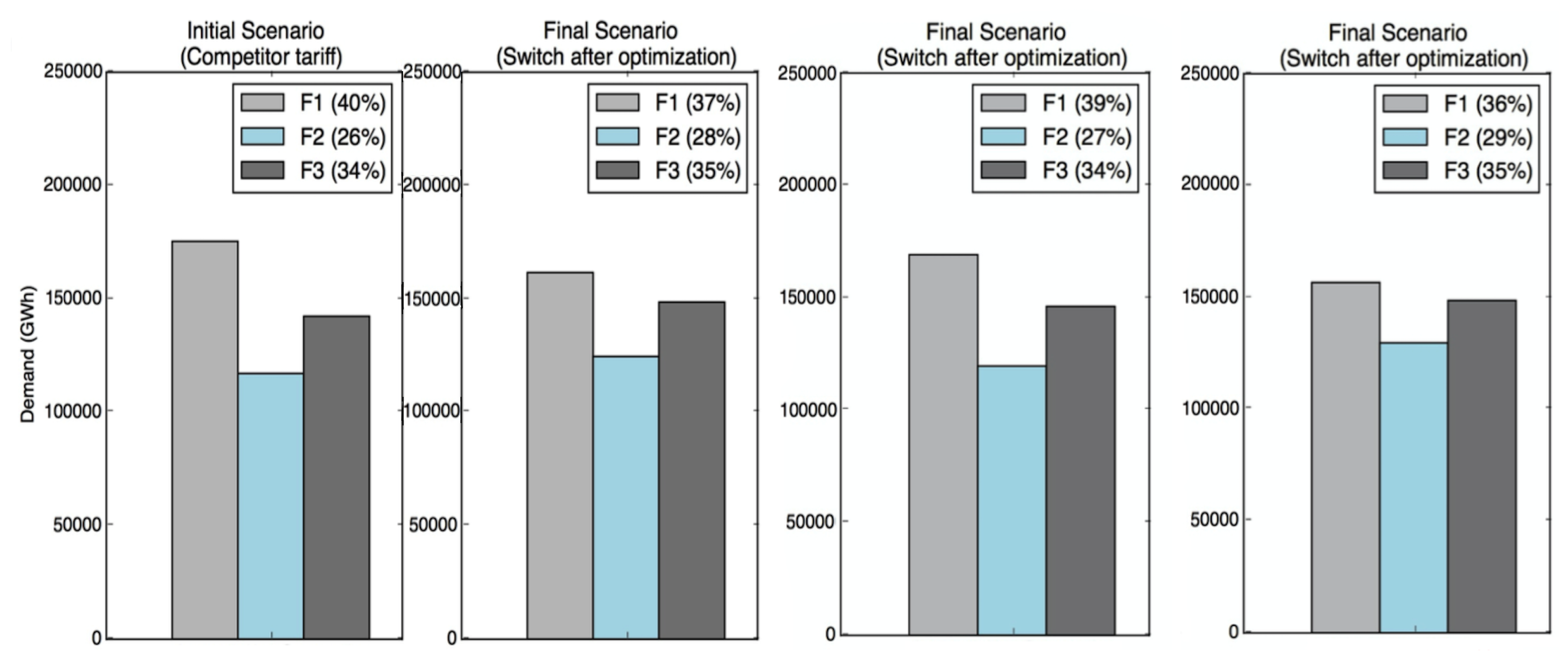
The flat rate case presents an estimated provider profit higher than the two-price case (e.g., around 1.40 M€ compared to around 1.30 M€ of the two-rate case for $ϵ$ = 1.0), with the savings a little less evenly spread among customer classes. It is interesting to observe that general improvements are possible by increasing elasticity; in particular, the profit is almost the same for $epsilon$ = 0.5 and $epsilon$ = 1.0 for both tariffs, but it increases for $epsilon$ = 1.5, with the new tariff, which is more beneficial for larger families, in both tariff cases. Such general improvements are possible since the increased elasticity enables a reduction of the wholesale electricity price via demand shifting. We can also notice that, with the highest elasticity factor, the price in $p_0$ is quite reduced with respect to the other cases. The cause of this behavior could be that the original demand distribution presents a peak in $p_2$, and residential customers are less prone to use electricity in $p_0$ (office hours). By increasing the elasticity factor, we increase the rate of demand shifts, and it causes a proportional growth of the loss factor. This leads to the need for more significant changes in optimal tariff prices to have a demand shift in the specific band (i.e., $p_0$) and to avoid the consumption loss for customers. We also show in Figure 5 the aggregate consumption shift among the bands and the distribution of consumption per band over the total aggregate residential consumption by increasing and decreasing the elasticity factor $ϵ$ in the two-price rate (the most common in the Italian market). We can see a local, but interesting peak of consumption in the third band. By increasing $ϵ$, we can notice a redistribution of residential aggregate loads, but we have to consider that, in the residential model, users decide to change tariff by loosing a certain quantity of consumption (see Table 2) to obtain lower prices.

4.4.2. Overhead Costs

Since several parameters of our model have been extrapolated from data, it is reasonable (and very interesting) to wonder what the effect of changing such parameters would be. Therefore, we have tried to investigate the effect of changing the value of the fixed overhead costs.

The value of the overhead $o_j$ is a major component of the electricity cost for the provider, and it can have a strong impact on the profit margin. We have changed the fixed overhead costs from 250 K€/GWh (see Section 3.6) down to 100 and up to 340. The results of this evaluation are reported in

Table 5. Effect of changing the fixed overhead costs.

Competitor		Prices			% Switch					Profit
Tariff	${\mathbf{o}}_{\mathbf{j}}$	${\mathbf{p}}_0$	${\mathbf{p}}_1$	${\mathbf{p}}_2$	${\mathbf{k}}_0$	${\mathbf{k}}_1$	${\mathbf{k}}_2$	${\mathbf{k}}_3$	${\mathbf{k}}_4$	(M€)
flat	100	324	281	325	71.4	71.7	70.9	73.5	73.9	6.67
flat	220	328	300	360	58.6	58.4	57.3	63.8	64.2	2.33
flat	250	334	312	363	52.2	52.0	50.7	58.0	58.5	1.40
flat	280	343	328	362	41.8	41.6	40.3	47.6	48.1	0.61
flat	340	–	–	–	–	–	–	–	–	–
two-price	100	334	273	316	71.3	71.3	70.8	73.5	73.8	6.54
two-price	220	338	293	351	57.9	57.8	56.9	63.5	63.9	2.21
two-price	250	344	305	353	51.0	51.0	50.0	57.4	57.9	1.30
two-price	280	353	323	352	39.3	39.6	39.0	46.2	46.9	0.53
two-price	340	–	–	–	–	–	–	–	–	–

, which shows the overhead value (in K€/GWh), the prices of the optimized new tariff (in K€/GWh), the percentage of switching customers for each class and the provider profit. When the overhead is low, the profit margin is very high, and it is possible to lower the prices to the point that the new tariff is competitive for all customer classes. As the overhead grows, attracting customers becomes increasingly difficult (see the fraction of switching customers), and the optimal prices become less convenient for customers. For large overhead (i.e., 340 K€/GWh), there is no economic advantage in attracting customers to the new tariff. The provider profit is higher in the case of the flat rate.

4.4.3. Perception Accuracy Parameters

We have also investigated the effect of changing the perception accuracy parameters by repeating our experiments with lower overhead costs, i.e., 220 and 100 K€/GWh. In particular, besides the initial setup with ${\beta }_k=0.75$, we have performed experiments with ${\beta }_k=1.0$ (i.e., a quite accurate perception, at the relevant range) and ${\beta }_k=1.25$ (i.e., bias toward underestimated variations) for both tariffs. The results are reported in

Table 6. Effect of changing the perception accuracy parameters and the overhead costs.

Competitor			Prices			% Switch					Profit
Tariff	${\mathbf{o}}_{\mathbf{j}}$	${\mathit{\beta }}_{\mathit{k}}$	${\mathbf{p}}_0$	${\mathbf{p}}_1$	${\mathbf{p}}_2$	${\mathbf{k}}_0$	${\mathbf{k}}_1$	${\mathbf{k}}_2$	${\mathbf{k}}_3$	${\mathbf{k}}_4$	(M€)
flat	250	0.75	334	312	363	52.2	52.0	50.7	58.0	58.5	1.40
flat	250	1.0	194	284	649	53.8	54.7	42.5	69.6	68.8	1.55
flat	250	1.25	115	320	650	59.6	58.7	43.7	62.3	59.9	1.77
flat	220	0.75	328	300	360	58.6	58.4	57.3	63.8	64.2	2.33
flat	220	1.0	131	266	649	59.7	59.9	49.5	72.5	71.8	2.48
flat	220	1.25	120	301	649	64.1	63.1	50.5	66.7	64.9	2.68
flat	100	0.75	324	281	325	71.4	71.7	70.9	73.5	73.9	6.67
flat	100	1.0	320	260	343	70.9	70.8	69.9	74.4	74.8	6.64
flat	100	1.25	144	241	649	73.9	72.7	64.6	76.0	74.9	6.84
two-price	250	0.75	344	305	353	51.0	51.0	50.0	57.4	57.9	1.30
two-price	250	1.0	121	290	630	50.2	53.2	44.1	69.6	69.2	1.43
two-price	250	1.25	95	326	630	56.5	56.9	44.7	62.5	60.7	1.65
two-price	220	0.75	338	293	351	57.9	57.8	56.9	63.5	63.9	2.21
two-price	220	1.0	136	272	630	57.1	58.8	50.9	72.5	72.2	2.35
two-price	220	1.25	88	307	630	61.7	61.8	51.5	66.9	65.6	2.55
two-price	100	0.75	334	273	316	71.3	71.3	70.8	73.5	73.8	6.54
two-price	100	1.0	330	253	334	70.8	70.7	69.8	74.3	74.7	6.52
two-price	100	1.25	159	246	630	72.8	72.2	65.3	76.2	75.4	6.71

. Apparently, customers that are less prone to overestimation are more difficult to manage for an energy provider, either because they are better capable of exploiting prices (due to accurate perception) or they are likely to cause wholesale price increases (due to their underestimated variations): to obtain tariffs that are beneficial for both the provider and the customers, the provider has to lower the prices in the first band and to increase them in the third one (where the peak is present) to find an economically favorable tariff with an increase of profit. The trend of obtaining higher profits by lowering overhead costs is respected, and we can notice another trend of obtaining higher profits by growing the underestimated variations of user consumption.

Finally, to underline the contribution of cognitive user aspects, we performed a test by considering changes of the customer elasticity factor in relation to the accuracy of their perceived consumption. We show the results in

Table 7. Effect of changing the perception accuracy parameters and the elasticity factor.

Competitor			Prices			% Switch					Profit
Tariff	$\mathit{ϵ}$	${\mathit{\beta }}_{\mathit{k}}$	${\mathbf{p}}_0$	${\mathbf{p}}_1$	${\mathbf{p}}_2$	${\mathbf{k}}_0$	${\mathbf{k}}_1$	${\mathbf{k}}_2$	${\mathbf{k}}_3$	${\mathbf{k}}_4$	(M€)
flat	1.5	0.75	72	303	649	56.5	56.9	42.8	66.0	64.5	1.68
flat	1.5	1.0	73	350	649	66.2	64.2	47.9	53.9	47.6	1.92
flat	1.5	1.25	75	393	625	71.9	69.1	56.4	46.9	34.0	1.97
flat	1.0	0.75	334	312	363	52.2	52.0	50.7	58.0	58.5	1.40
flat	1.0	1.0	194	284	649	53.8	54.7	42.5	69.6	68.8	1.55
flat	1.0	1.25	115	320	650	59.6	58.7	43.7	62.3	59.9	1.77
flat	0.5	0.75	340	329	345	53.7	53.7	53.4	55.9	56.1	1.42
flat	0.5	1.0	339	324	349	53.2	53.1	52.6	56.5	56.8	1.41
flat	0.5	1.25	337	318	546	52.7	52.6	51.7	57.1	57.5	1.41
two-price	1.5	0.75	75	310	630	53.1	55.2	44.1	66.1	65.1	1.55
two-price	1.5	1.0	88	356	630	63.7	62.3	48.0	54.1	48.8	1.81
two-price	1.5	1.25	96	393	615	71.6	68.7	56.3	46.2	32.9	1.87
two-price	1.0	0.75	344	305	353	51.0	51.0	50.0	57.4	57.9	1.30
two-price	1.0	1.0	121	290	630	50.2	53.2	44.1	69.6	69.2	1.43
two-price	1.0	1.25	95	326	630	56.5	56.9	44.7	62.5	60.7	1.65
two-price	0.5	0.75	350	321	336	52.5	52.7	52.7	55.3	55.6	1.30
two-price	0.5	1.0	349	317	340	52.0	52.1	51.9	55.8	56.3	1.31
two-price	0.5	1.25	347	311	346	51.5	51.6	51.0	56.5	57.0	1.30

. Differently from [14], which only considers customer elasticity and load consumption, we show that perception accuracy can significantly affect the demand response model. The general result of [14] is a lower provider profit for more elastic customers, and on the other hand, more inelastic customers tolerate price increases without reducing considerably the consumption, thus generating higher profits. In our work, we also consider the perception accuracy of consumption for each customer, and we can observe different tradeoffs. In particular, we have interesting and different trends by increasing ${\beta }_k$: for higher values of $\beta$, we can observe an increase of provider profit and a higher percentage switch of more elastic customers. This is due to user capacity to better exploit prices (for accurate perception ${\beta }_k$ = 1.0) and to their underestimated variations (for ${\beta }_k$ = 1.25). The increase of ${\beta }_k$ influences the flexibility to shift consumption. With $ϵ$ factor = 0.5, the change in perception accuracy has no effect on profit in both tariff cases. This is because the less elasticity does not allow consumption shifts that make it interesting to move towards a new tariff for users. Moreover, by increasing $ϵ$, consumers are more prone to switch to a new competitive tariff, and this causes a general increase of provider profit. We can observe that the contribution of perception accuracy is very important to define a relation between customer elasticity and provider profit with higher profits for higher values of ${\beta }_k$. From this perspective, awareness tools for users on energy consumption can have significant potential to change behavior on energy usage with a reduction of energy consumption which could be achieved through the implementation of this measure.

4.5. Experimental Results of the Deterministic Model

We focused on the first scenario, and we have investigated the effect of changing the elasticity factor and the value of the fixed overhead costs from 250 K€/GWh (see Section 3.6) down to 100 and up to 340. We consider also a third tariff case (referred to as the band rate), which is a close match for tariffs employed for industrial electricity contracts in the Italian market. Optimal prices for flat rate, two-price rate and band rate are reported in

Table 8. Effect of changing the overhead costs (deterministic model).

Competitor		Prices			${\mathbf{y}}_{{\mathbf{k}}_{\mathbf{k}},0}$
Tariff	${\mathbf{o}}_{\mathbf{j}}$	${\mathbf{p}}_0$	${\mathbf{p}}_1$	${\mathbf{p}}_2$	${\mathbf{k}}_0$	${\mathbf{k}}_1$	${\mathbf{k}}_2$	${\mathbf{k}}_3$	${\mathbf{k}}_4$
flat	100	341	335	352	1.0	1.0	1.0	1.0	1.0
flat	250	390	100	191	1.0	1.0	1.0	1.0	0.0
flat	280	559	90	366	1.0	1.0	0.0	1.0	1.0
flat	340	400	150	650	0.0	1.0	0.0	0.0	1.0
two-price	100	357	322	339	1.0	1.0	1.0	1.0	1.0
two-price	250	356	90	167	1.0	1.0	1.0	1.0	0.0
two-price	280	563	72	357	0.0	1.0	0.0	0.0	1.0
two-price	340	690	320	274	0.0	0.0	0.0	1.0	0.0
band-prices	100	334	323	356	1.0	1.0	1.0	1.0	1.0
band-prices	250	590	250	194	1.0	1.0	1.0	1.0	0.0
band-prices	280	550	90	363	0.0	1.0	0.0	1.0	1.0
band-prices	340	519	72	690	0.0	0.0	0.0	0.0	1.0

, which shows also the user switch to the new optimal tariff (i.e., $y_{k_k,i}=1.0$ if the user k switches to the new tariff). The most interesting case is the experiment with large overheads (i.e., 280 and 340): there is no economic advantage in attracting all customers to the new tariff. In these cases, we can also see a relation between users that remain in the competitor tariff and their self-elasticity (i.e., the amount of consumption to distribute among the other bands).

For the elasticity factor, it is important to underline that we consider a loss factor of 0% for all users (i.e., we have only a shift of total consumption among the bands without a loss as in the residential model). We show in

Table 9. Effect of changing the elasticity factor (deterministic model).

Competitor		Prices
Tariff	$\mathbf{ϵ}$	${\mathbf{p}}_0$	${\mathbf{p}}_1$	${\mathbf{p}}_2$
flat	0.5	316	269	439
flat	1.0	390	100	191
flat	1.5	604	72	338
two-price	0.5	330	264	421
two-price	1.0	356	90	167
two-price	1.5	530	75	330
band-prices	0.5	311	300	438
band-prices	1.0	590	250	194
band-prices	1.5	594	100	340

the new optimal prices by changing the elasticity factor $ϵ$. We do not report the value of ($y_{k_k,i}$) for user tariff switch because in the considered case (i.e., with $o_j=250$), the new optimal tariff attracts all of the users.

To underline the importance of the elasticity factor, we also show in Figure 6 the shift of aggregate consumption among the bands by changing $ϵ$ with the two-price rate (the most common rate in the Italian market). With $ϵ=0.5$, there is a very small change in the distribution of consumption among the bands. The consumption shifts grow proportionally with the growth of the elasticity factor as expected. It is interesting to notice that the industrial consumption peak is located in the first band, and it decreases with larger elasticity. In this deterministic case, we assume implicitly that consumers are more rational and that they shift their consumption if they have economic benefits.

4.6. A Real-World Case Study

The optimization model presented in the paper provides the basis for some of the decision support tools implemented in the DAREED online platform. DAREED was a FP7 project aiming at the definition and implementation of a comprehensive web-based system to coordinate the efforts of citizens, policy makers and energy providers for improving the energy efficiency of a district. During its validation stage, a prototype of the platform had been used by more than 200 users, including 34 energy providers and 13 policy makers.

The DAREED platform included (A working prototype is still running and available at the moment of writing this paper, but it may be discontinued in the following months. The prototype can be accessed at: http://demo.dareed.eu) three tools that were based on our model: two of them were addressed to energy providers and one to local policy makers. In detail, energy providers had access to:

• A tool for suggesting tariffs for districts, which could provide price recommendation for ToU-based tariffs, via the stochastic version of our optimization model.
• A similar tool for suggesting tariffs for buildings, which could be used to define tailored tariffs for large electricity consumers and was based on the deterministic version of our model.

Policy makers could instead access a tool for identifying the optimal values of the behavioral parameters of citizens in a district, i.e., their cross-elasticity matrix, their perception accuracy and their risk aversion. In this latter case, our model was optimized over fixed prices, and the decision variables were the ${ϵ}_{i,h}$, ${\beta }_k$, ${\rho }_k$ parameters.

For a whole description of the three decision support tools, we refer to Deliverable 5.3 (http://www.dareed.eu/251). In the remainder of this section, we focus on the first tool (i.e., obtaining tariff recommendations at district level), and we discuss how it has been used to obtain valuable results in the context of the project.

From the perspective of our model, providing this kind of recommendation required obtaining information about: (1) the available prices bands, (2) yearly consumption over the considered district, (3) behavioral parameters for all customer classes and (4) prices for pre-existing tariffs. The definition of price bands is usually subject to national regulations, and the DAREED platform supported a sample of the existing ones in Italy, England and Spain. All decision support systems were connected with a hub for collecting real-time electricity monitoring data, which was integrated with statistical considerations to estimate consumption figures for all customer classes in a district. The platform also featured a market place section to exchange requests and offers between citizens, energy providers and policy makers: this market place represented an excellent source of information to obtain a proper configuration of the customer elasticity, perception accuracy and risk aversion parameters. Finally, prices for the existing tariffs had to be specified manually by the user. Once all relevant information had been obtained, the decision support tool would solve our optimization model and provide solutions. The user could then inspect the outcomes, which contained the price recommendations for the new tariff, an indication of whether the tariff was attractive enough for the customers and an estimate of how the users’ energy demand was likely to shift due to the new prices.

The described tool has been employed in the final stage of the project by staff at ENEL [34] to perform a case study and assess how to design an attractive tariff for an Italian town that was one of the project pilots. More in detail, in the period between 1 January 2017 and 30 June 2018, twenty million Italian households and small businesses were required to switch their electricity tariff, as the last stage of a market liberalization process that spanned multiple years. This massive transition represented a huge opportunity for energy providers, but also one that was very difficult to exploit, since competition and taxes had progressively cut the profit margin. In this context, a model such as the one we have presented could provide a significant advantage.

Specifically, project participants from ENEL employed the decision support tool that we have described to obtain tariff recommendations for the municipality of Lizzanello, in southern Italy. The use of the tool allowed them to understand how to define the prices so as to beat the most representative tariffs offered by competitors and to assess the share of new customers that were likely to make switch: in this case, from 22% to 75%, depending on how much profit they were willing to sacrifice in order to obtain new customers. Even in the lowest-prices, largest-number-of-customers scenario (i.e., the 75% switch), the estimated profit per customer was of 75 €/year: a small budget, but enough to support marketing efforts for (more profitable) added value services.

5. Conclusions

In this work, we have devised a non-linear optimization model for optimizing ToU-based tariffs for electricity. We have developed two versions of our model (i.e., stochastic and deterministic) with different application fields. Overall, our model is rather comprehensive and takes into account: (1) the presence of multiple tariffs and (most importantly) competitors, (2) the demand response behavior of the customers, (3) the effect of demand shifts on the wholesale energy price and, finally, (4) cognitive aspects of the customers (in particular, their risk aversion and the accuracy of their consumption estimates). The problem objective is to maximize the provider profit.

We have modified our model for two additional and relevant use cases. First, the deterministic model could be used to support the definition of tailored tariffs for public buildings or large industrial customers. A second use case consists of employing the model to obtain recommendations about changes in the customer behavior parameters (e.g., elasticity, perception accuracy). This alternative use case may be particularly appealing for policy makers to devise incentive schemes or awareness campaigns to increase the perception accuracy about consumption.

From our results of the residential stochastic model, we notice a strong relation between perception accuracy and consumption shifts. Thus, the contribution of perception accuracy is very important to define a relation between customer elasticity and provider profit. Awareness tools on energy consumption have significant potential to change behavior on energy usage. Moreover, the elasticity factor is an important parameter to obtain peak reductions by distributing the user consumption among the bands to have economic benefits. We have also tested the optimization model in a real setting in the context of the FP7 DAREED project, where the model has been employed to provide tariff recommendations or to help the identification of goals for local policies.

We are improving some components in our model. In particular, our perception model could be made more flexible and validated on real data. The elastic model that we employ for demand shifting could be augmented to take into account limits to the maximal acceptable variation or to take into account the comfort loss/gain due to changes in the net energy consumption. We are also considering the possibility to split the yearly consumption into multiple months, which would allow one to model different types of tariffs and to (partially) take into account weather conditions. We are confident that we could provide support for a wider range of tariff schemes (e.g., discounted rates).

References

- Albadi, M.; El-Saadany, E. Demand response in electricity markets: An overview. In Proceedings of the IEEE Power Engineering Society General Meeting, Tampa, FL, USA, 24–28 June 2007; pp. 1–5. [Google Scholar]
- Albadi, M.; El-Saadany, E. A summary of demand response in electricity markets. Electr. Power Syst. Res. 2008, 78, 1989–1996. [Google Scholar] [CrossRef]
- Palensky, P.; Dietrich, D. Demand Side Management: Demand Response. Intell. Energy Syst. Smart Loads 2011, 7, 381–388. [Google Scholar]
- Torriti, J. The Risk of Residential Peak Electricity Demand: A Comparison of Five European Countries. Energies 2017, 10, 385. [Google Scholar] [CrossRef]
- Lujano-Rojas, J.M.; Monteiro, C.; Dufo-López, R.; Bernal-Agustín, J.L. Optimum residential load management strategy for real time pricing (RTP) demand response programs. Energy Policy 2012, 45, 671–679. [Google Scholar] [CrossRef]
- Molderink, A.; Bakker, V.; Bosman, M.G.C.; Hurink, J.L.; Smit, G.J.M. Management and Control of Domestic Smart Grid Technology. IEEE Trans. Smart Grid 2010, 1, 109–119. [Google Scholar] [CrossRef]
- Eissa, M. Demand side management program evaluation based on industrial and commercial field data. Energy Policy 2011, 39, 5961–5969. [Google Scholar] [CrossRef]
- Ventosa, M.; Baillo, A.; Ramos, A.; Rivier, M. Electricity market modeling trends. Energy Policy 2005, 33, 897–913. [Google Scholar] [CrossRef]
- Vardakas, J.S.; Zorba, N.; Verikoukis, C.V. A survey on demand response programs in smart grids: Pricing methods and optimization algorithms. IEEE Commun. Surv. Tutor. 2015, 17, 152–178. [Google Scholar] [CrossRef]
- Aalami, H.; Moghaddam, M.P.; Yousefi, G. Demand response modeling considering Interruptible/Curtailable loads and capacity market programs. Appl. Energy 2010, 87, 243–250. [Google Scholar] [CrossRef]
- Aalami, H.; Moghaddam, M.P.; Yousefi, G. Modeling and prioritizing demand response programs in power markets. Electr. Power Syst. Res. 2010, 80, 426–435. [Google Scholar] [CrossRef]
- Conejo, A.; Morales, J.; Baringo, L. Real-time demand response model. IEEE Trans. Smart Grid 2010, 1, 236–242. [Google Scholar] [CrossRef]
- Luo, Z.; Hong, S.H.; Kim, J.B. A Price-Based Demand Response Scheme for Discrete Manufacturing in Smart Grids. Energies 2016, 9, 650. [Google Scholar] [CrossRef]
- Yusta, J.; Ramírez-Rosado, I.; Dominguez-Navarro, J.; Perez-Vidal, J. Optimal electricity price calculation model for retailers in a deregulated market. Int. J. Electr. Power Energy Syst. 2005, 27, 437–447. [Google Scholar] [CrossRef]
- Kirschen, D.S.; Strbac, G.; Cumperayot, P.; de Paiva Mendes, D. Factoring the elasticity of demand in electricity prices. IEEE Trans. Power Syst. 2000, 15, 612–617. [Google Scholar] [CrossRef]
- Torriti, J. Price-based demand side management: Assessing the impacts of time-of-use tariffs on residential electricity demand and peak shifting in Northern Italy. Energy 2012, 44, 576–583. [Google Scholar] [CrossRef]
- Samadi, M.; Javidi, M.H.; Ghazizadeh, M.S. The effect of time-based demand response program on LDC and reliability of power system. In Proceedings of the 21st Iranian Conference on Electrical Engineering (ICEE), Mashhad, Iran, 14–16 May 2013; pp. 1–6. [Google Scholar]
- Bartusch, C.; Wallin, F.; Odlare, M.; Vassileva, I.; Wester, L. Introducing a demand-based electricity distribution tariff in the residential sector: Demand response and customer perception. Energy Policy 2011, 39, 5008–5025. [Google Scholar] [CrossRef]
- Siebert, L.C.; Sbicca, A.; Aoki, A.R.; Lambert-Torres, G. A Behavioral Economics Approach to Residential Electricity Consumption. Energies 2017, 10, 768. [Google Scholar] [CrossRef]
- Lijesen, M. The real-time price elasticity of electricity. Energy Econ. 2007, 29, 249–258. [Google Scholar] [CrossRef]
- Borenstein, S. To What Electricity Price Do Consumers Respond? Residential Demand Elasticity Under Increasing-Block Pricing. 2009. Available online: http://faculty.haas.berkeley.edu/borenste/download/NBERSI2009.pdf (accessed on 8 September 2017).
- Ito, K. Do Consumers Respond to Marginal or Average Price? Evidence from Nonlinear Electricity Pricing. Am. Econ. Rev. 2014, 104, 537–563. [Google Scholar] [CrossRef]
- Attari, S.; DeKay, M.; Davidson, C.; Bruin, W.D. Public perceptions of energy consumption and savings. Proc. Natl. Acad. Sci. USA 2010, 107, 16054–16059. [Google Scholar] [CrossRef] [PubMed]
- Ramos, A.; Ventosa, M.; Rivier, M. Modeling competition in electric energy markets by equilibrium constraints. Util. Policy 1999, 7, 233–242. [Google Scholar] [CrossRef]
- Zheng, R.; Xu, Y.; Chakraborty, N.; Sycara, K. Crowdfunding Investment for Renewable Energy. In Proceedings of the AAMAS ’15 International Foundation for Autonomous Agents and Multiagent Systems, Richland, SC, USA, 4–8 May 2015; pp. 1751–1752. [Google Scholar]
- Baboli, P.T.; Eghbal, M.; Moghadda, M.P.; Aalami, H. Customer behavior based demand response model. In Proceedings of the Power and Energy Society General Meeting, San Diego, CA, USA, 22–26 July 2012; pp. 1–7. [Google Scholar]
- De Filippo, A.; Lombardi, M.; Milano, M. Non-linear Optimization of Business Models in the Electricity Market. In Proceedings of the Integration of AI and OR Techniques in Constraint Programming: 13th International Conference, Banff, AB, Canada, 29 May–1 June 2016; pp. 81–97. [Google Scholar]
- Winston, W. Operations Research: Applications and Algorithms; PWS-Kent Pub. Co: Belmont, CA, USA, 2004; Volume 3. [Google Scholar]
- Lombardi, M.; Milano, M.; Bartolini, A. Empirical decision model learning. Artif. Intell. 2017, 244, 343–367. [Google Scholar] [CrossRef]
- Choi, S.; Fisman, R.; Gale, D.; Kariv, S. Consistency and Heterogeneity of Individual Behavior under Uncertainty. Am. Econ. Rev. 2007, 97, 1921–1938. [Google Scholar] [CrossRef]
- Authority, E.; Italian Energy Market Manager (GME). Riforma Della Tariffa Domestica; Technical Report; Autorità per l’energia elettrica, il gas ed il sistema idrico: Rome, Italy, 2014. [Google Scholar]
- Beale, E.M.L.; Forrest, J.J.H. Global optimization using special ordered sets. Math. Program. 1976, 10, 52–69. [Google Scholar] [CrossRef]
- Scalari, S.; (Enel Engineering and Research, Pisa, Italy). Personal communication, 2015.
- Guidi, L.; (Enel Engineering and Research, Pisa, Italy). Personal communication, 2017.
Figure 1.
Location of this work in the current state of the art.
Figure 2.
Perception model.
Figure 3.
Interpretation of the cross-elasticity matrix.
Figure 4.
Wholesale electricity price over demand, Italian market (2013).
Figure 5.
Aggregate consumption among the tariff bands before the switch (left) and after the switch to the new optimized tariff (two-price rate) with respectively , and .
Figure 6.