Modeling a Hybrid Microgrid Using Probabilistic Reconfiguration under System Uncertainties


1
Computer and Electrical Engineering Department, Florida Atlantic University, Boca Raton, FL 33431, USA
2
Ocean and Mechanical Engineering Department, Florida Atlantic University, Boca Raton, FL 33431, USA
*
Author to whom correspondence should be addressed.
Energies 2017, 10(9), 1430; https://doi.org/10.3390/en10091430
Submission received: 10 August 2017
/
Revised: 2 September 2017
/
Accepted: 16 September 2017
/
Published: 18 September 2017
(This article belongs to the Section F: Electrical Engineering)
Abstract
:A novel method for a day-ahead optimal operation of a hybrid microgrid system including fuel cells, photovoltaic arrays, a microturbine, and battery energy storage in order to fulfill the required load demand is presented in this paper. In the proposed system, the microgrid has access to the main utility grid in order to exchange power when required. Available municipal waste is utilized to produce the hydrogen required for running the fuel cells, and natural gas will be used as the backup source. In the proposed method, an energy scheduling is introduced to optimize the generating unit power outputs for the next day, as well as the power flow with the main grid, in order to minimize the operational costs and produced greenhouse gases emissions. The nature of renewable energies and electric power consumption is both intermittent and unpredictable, and the uncertainty related to the PV array power generation and power consumption has been considered in the next-day energy scheduling. In order to model uncertainties, some scenarios are produced according to Monte Carlo (MC) simulations, and microgrid optimal energy scheduling is analyzed under the generated scenarios. In addition, various scenarios created by MC simulations are applied in order to solve unit commitment (UC) problems. The microgrid’s day-ahead operation and emission costs are considered as the objective functions, and the particle swarm optimization algorithm is employed to solve the optimization problem. Overall, the proposed model is capable of minimizing the system costs, as well as the unfavorable influence of uncertainties on the microgrid’s profit, by generating different scenarios.
1. Introduction
Energy generation development, increasing interests toward environmental aspects, and improving the power system reliability provide enough motivation to change the distribution systems’ mode from inactive to active, and increase distributed energy resources’ (DERs) penetration in the microgrid (MG) environment [1,2]. A MG is described as a small-scale distribution grid that consists of diversified distributed generation units, energy storage systems (ESSs), and local controllable loads that typically can either be operated in islanded or grid-tied modes. A grid-connected MG is tied to the upstream utility grid through a point of common coupling (PCC), in order to exchange power. More than that, providing voltage support as an ancillary service to the main distribution network is another advantage of a MG system compared with conventional end-user units [3,4]. Since a MG can operate autonomously, in the case of events such as brownout or blackout, it is capable of managing the operation of a localized power system [5].
The smart grid is a novel concept that has become apparent in recent years. It is an intelligent energy system that consists of a variety of advanced energy resources/loads such as smart appliances, energy efficient and renewable energy resources, smart meters, and electric cars [6,7,8]. The originality of a smart grid is that it can request to improve operations, maintenance and scheduling by assuring that each component of the ingenious electric grid have the ability of both ‘talk’ and ‘listen’. The infrastructure of energy grids are growing to be more advanced in terms of power production, data sharing and management, automation, and communication with intricate and fully united network. Therefore, intelligent management applications and services should follow in a way that attains the system objectives corresponding to supply/demand balance, utility maximization, energy saving, and operational cost reduction [9,10,11].
Also, the concept of a demand response (DR) program has been implemented to reduce or shift the energy usage at peak times, which can reduce utility electric bills, and also provide a higher capacity factor and distribution grids security at the same time [12,13]. Basically, DR is defined as behavioral changes in electric consumption implemented directly or indirectly by customers or end users from their regular usage/injection templates in response to determined signals. The establishment of time-differentiated pricing, such as time-of-use (TOU) and real-time pricing (RTP) and the incentive-based DR contracts that can be offered to the customers drives the paradigm shifting, in which the wholesale price fluctuations will be reflected to the end users and will motivate curtailment and responsive load shifting [14]. In emergency cases, a MG is often needed to reconfigure itself as soon as possible in order to support steady electricity to critical loads. Different types of operations, including topology switching, load shedding, and generation regulation, are discussed in the reconfiguration concept. Therefore, the problem of reconfiguration becomes a generic constrained nonlinear optimal problem [15].
This paper addresses optimal energy scheduling/management matters in a grid-tied MG reconfiguration as a fundamental problem in interactive smart grids operation, with consideration of load and renewable resources uncertainties. Previous research studies have discussed the scheduling of distributed generation (DG) operations and loads in MGs [2,16]. Also, a three-stage optimal method for economic dispatch of the power system using sensitive factors, improved direct search method, and the incremental linear models is presented in [17]. However, the current study focuses on the central problem of uncertainty in the predicted load demand and renewable energy units in the presence of a battery storage system in a MG environment. MG operation and management approaches are discussed and analyzed that consider the intermittent nature of renewable energy resources by utilizing stochastic methods in order to solve the problem. A stochastic energy-planning modeling for a MG, including plug-in electric vehicles and intermittent renewable energy units, has been proposed in [18,19] in order to minimize the power losses and operational cost. Participation of a typical MG in the electricity market under certain policies of power market using hierarchical scheduling and genetic algorithm-based methods in order to obtain the economic evaluation and reduce uncertainties of the proposed system are discussed in [16,20]. Also, different multi-time scale control strategies that deploy electric vehicle demand flexibility in order to solve grid unbalancing and congestions [21], reduce demand charges, and effectively address renewable energies production uncertainties, are discussed [22].
In [23], a scenario-robust mixed integer linear programing was modeled to employ ensemble weather forecasts for the performance improvement of a hybrid MG comprising both renewable and conventional power sources. The model was exercised to quantify the privilege of utilizing ensemble weather forecasts, and the optimal performance of a hypothetical power grid, including wind turbines, is predicted by employing simulated scenarios of realistic weather forecasts based on data. The comprehensive financial dispatch problem of a MG employing four various optimization techniques comprising lambda logic, lambda iteration, direct search method (DSM), and particle swarm optimization (PSO) under different test systems and control areas is discussed in [24]. Also, [25] proposes and designs a centralized and decentralized demand–response-based multi-agent control and scheduling model, including load curtailment and a backup diesel power generation, in order to measure end-user satisfaction.
A distributed algorithm using the classical symmetrical assignment problem is resolved in [26,27], where energy planning is modeled as a resource allocation problem, and distribution techniques are also discussed for distributed allocation. Furthermore, in [28], a convex problem formulation is described where a dual decomposition is utilized to develop a distributed energy management strategy (EMS) in MG systems in order to fulfill the energy balance of supply/demand.
Where the privacy constraints are associated with the linear programming approach and distributed algorithms are developed, a privacy-preserving energy planning technique in MGs can be found in [29]. Also, [30] focuses on the additive-increase and multiplicative-decrease algorithms are developed to find the optimal operation of DERs in a distributed procedure.
In this paper, an economic dispatch (ED) problem (fuel cost and generated emission minimization) of a MG containing both dispatchable and non-dispatchable DERs is formulated and modeled with diverse operational constraints. An energy planning in MGs is formulated specifically as an optimal power flow (OPF) problem. Solving the OPF problem is a complex task due to the non-convex constraints of power flow.
In summary, the main contributions of the paper can be expressed as follows:
- Among the formerly stated optimization techniques, PSO has been considerably applied in optimal operation planning problems, mostly because of its capability for population-based searches as well as its robustness, convergence speed, and simplicity. In this paper, the Monte Carlo (MC) simulation outcomes, along with the MG essential data, are considered as the input of a PSO algorithm, in order to find the day ahead optimal operation management of a MG, which has not been properly taken into account in the aforementioned research.
- The uncertainty of renewable energy resource and local load are considered, and the solution guarantees strength against all possible realizations of the modeled operational uncertainties.
- The existing model applies a probabilistic reconfiguration and unit commitment (UC) concurrently to attain the optimal set points of the generating units of the MG, in addition to the MG optimal topology for the next-day electricity market. The probabilistic reconfiguration and UC for a MG optimal energy planning, with the integration of renewable energy and load demand, is a novel operation to estimate MG’s profit in the uncertain situation. The proposed approach has the capability to be combined with uncertainty simulation models in order to obtain part of the required inputs.
This paper is organized as follows: The intermittent behavior of a solar PV system and electric load consumption are considered as uncertainties of the system, which are modeled through probability density functions. In Section 2, the MG architecture and associated generating units are modeled. Proposed objective functions and related uncertainties modeling are also presented in that section. The system’s technical and operational constraints are formulated is Section 3. Additionally, proposed optimal operation planning is carried out in Section 4. Simulation results and discussions on system behavior under different test conditions are presented in Section 4. Consequently, conclusions are given in the last section.
2. Microgrid Configuration
The application of each particular DER can create as many challenges as it may resolve; thus, a proper procedure to realize the emerging potential of DERs would address a system approach that considers generation and associated consumptions as a subsystem or a small-scale grid. Furthermore, the integration of DERs in a MG and the utilization of renewable energies in bulk amounts can enable related problems on economy, technology and environment to be attentively studied within the target system, and proper decisions to be made that improve the management of its exploitation.
The organic municipal waste, such as food waste, agricultural waste, municipal solid waste (MSW), and municipal sewage sludge (bio-solids), have been studied in many research studies that show their high potential for bioenergy extraction [31]. In recent years, microbial fuel cells (MFCs) have been perused for the generation of electricity [32] through utilizing reactors and anaerobic reformers that use bio-waste and natural gas as the input fuel, as shown in Figure 1. The proposed MG in this research is composed of a microturbine (MT), a fuel cells (FC) unit, a solar photovoltaic (PV) system, and an battery storage system (BSS). Also, a communication network is designed among energy resources, local demand, and the MG central controller (MGCC) in order to send power references and exchange data. The control structure relies on a MGCC to deliver the energy planning, and manages the OPF in the system to fulfill the local needs. The distribution system operator (DSO) takes the MGCC as one subsection, which is qualified to control a cluster of suppliers and flexible loads locally and allow renewable energy-based resources (REBG) to supply their full advantageousness, while minimizing the emission of energy components’ pollutants. The entire MG is connected to an upstream network through a PCC. Also, a smart meter device is located between the input energy and local load to record the consumption of electric energy in hourly intervals or less, and also to communicate that information back to the grid and MGCC for monitoring and billing. Smart meters are capable of bidirectional communication between the meter and the central system. The proposed MG configuration studied in this research is presented in Figure 1.
In the following sections, the proposed model objective functions consisting of operational cost functions and emission reduction functions are presented, which will be solved and minimized through employing the PSO algorithm.
2.1. First Objective Function: Operational Costs
One of the optimization goals of the MG utilization is to minimize operational costs. The total cost of the system is calculated by adding up the costs of each generating unit as the following equation:
where and are the operational costs of the FC and MT at time t, respectively. Additionally, , , and stand for the cost of solar PV, battery storage, and the cost of purchasing electricity from the main grid at time t, respectively. The cost of each generating resource is calculated based on its corresponding output power per hour. The considered operation cost includes the cost of generating power, fuel costs, and the operation and maintenance (O&M) costs of energy units.
The cost of generating energy by a MT can be calculated using the following equation:
where BG,MT, PMT, and are the MT generation costs in $/kW, the produced power in kW, and the on and off status of the MT, respectively. It is assumed that is one when the turbine is on, and is zero when the turbine is off. Also, the microturbine start-up cost can be calculated by the below equation:
where is the cost of turning the MT on and off in $. In addition, the cost of O&M by utilizing a micro-gas turbine can be presented as follows:
In the above equation, stands for the O&M cost of a MT unit in $/kW. In general, the total operation cost of a MT system can be calculated as in Equation (5).
Additionally, the operational cost of a FC unit is presented:
where BG,FC, PFC, and are the FC generation cost in $/kW, produced power in kW, and the on and off status of the FC, respectively. The is one when the fuel cell is on, and it is considered zero when the unit is off.
The FC start-up cost is also similar to the MT start-up cost equation, and it can be shown in Equation (7).
where is the cost of turning the FC on and off in $. Similarly, the O&M cost of a FC unit can be obtained using Equation (8).
where stands for the O&M cost of a FC unit in $/kW. Overall, the total operation cost of a FC system can be obtained as shown in Equation (9).
The cost of power production by a solar PV system is presented as following.
where BG,PV, PPV and stand for the PV generation cost in $/kW, produced power in kW, and the on and off status of the PV, respectively. Also, the O&M cost of a PV system can be shown as in Equation (11).
where represents the O&M cost of a PV unit in $/kW. In general, the operation cost of a solar PV system can be calculated as follows:
The operation cost of a BSS system includes the cost of output power delivery by the unit and the O&M cost of the battery energy storage system. The delivery power cost at the BSS output can be calculated as follows:
where PBSS, BBSS, and are the battery storage produced power in kW, the cost of power delivery at the BSS output in $/kW and the on and off status of the battery sets (which can be either one or zero), respectively. Moreover, the O&M cost of a BSS can be obtained using the below equation:
where stands for the O&M cost of a battery storage unit in $/kW. Overall, the total operation cost of a BSS is presented as follows:
The cost of purchasing electrical power from the upstream external grid is shown in Equation (16).
where Pbuy-grid and Bbuy-grid represent the amount of purchased power from the main grid in kW, and the power unit price of electricity in $/kW, respectively.
2.2. Second Objective Function: Generated Emission
The amount of greenhouse gases (GHG) generated by energy resources is another factor that can be minimized in order to optimize the operation of a MG. Thus, the second objective function proposed in this paper is expressed as follows:
where , , and are the amount of emission produced by FC, MT, and BSS during the operation time, respectively.
The pollution generated in the environment by the non-renewable resources are mainly three GHGs including carbon dioxide (CO2), nitrogen dioxide (NOx) and sulfur dioxide SO2. The quantity of emissions produced by operating a FC unit, a MT, and BSS, respectively, can be calculated using the below equations [33]:
where stands for the amount of emissions generated by each conventional DER in kg/kWh, and can be expressed as follows:
In Equation (21), CO2(t), SO2(t), and NOx(t) are the amounts of carbon dioxide, nitrogen oxides, and sulfur dioxide emissions produced by units at the time t, respectively.
2.3. Uncertainties in Solar Radiation and Load
Renewable DG resources i.e., PV or wind turbine are non-dispatchable, and their output power is a function of the availability of the primitive sources (such as solar irradiance or wind speed etc.). Therefore, the output of such units is assumed to be random variables because of the stochastic nature of renewable DERs, and no generation cost would be considered for their production during the operation period. In this paper, the uncertainty is modeled utilizing MC simulation, where for uncertain inputs, i.e. solar radiation and load demand, some scenarios are created. Subsequently, the system is studied under obtained stochastic scenarios as deterministic inputs. Thus, there are different statuses, which are analyzed by using different scenarios. In order to calculate scenario aggregation, the expected value (h) is employed.
where is the probability of each scenario, is the value of variables in each scenario, and is number of scenarios. Also, the coefficient of variance (Cvx) is defined as follows.
where σx and μx are the standard deviation and mean value of parameter x, respectively. If Cvx is less than a specific tolerance, the result will be relatively acceptable.
Since solar power output has an intermittent nature and the solar radiation has a high degree of uncertainty, the sun radiation needs to be presented as a probability function. Variation in solar radiation is dependent on diverse factors such as weather conditions, the time of the day, month and season; the panels’ tilt angle, or the orientation of the PV solar cells to the sun radiation. The probability density function (PDF) of solar radiation is modeled using the beta density as the following [34]:
where S and represent solar radiation in W/m2 and the gamma distribution function, respectively. Also, αβ, and ββ are parameters of the beta probability distribution function in kW/m2, and calculated utilizing the mean () and standard deviation () of solar irradiance s as following:
In addition, the behavioral patterns of various electric consumers lead to an alteration in the load demand profile in MG systems. By employing statistical analysis, the created alterations can be attained. Since electric consumption changes continually with a high level of uncertainty, in this paper, load demand is considered as a normal distribution function with a mean value and a standard deviation as follows [35].
where and are the mean and standard deviation of the load, respectively. Also, Pd represents the power demand. In this paper, the uncertainty is modeled utilizing a MC simulation so that for uncertain inputs, i.e. solar radiation, temperature, and load demand, numerous scenarios are created. Therefore, the system is studied under achieved stochastic scenarios as deterministic inputs. Therefore, there are various statuses, which are analyzed by using distinctive scenarios. In fact, the MC technique is an approach that utilizes stochastic variables and their related PDFs to solve the uncertainty problems.
3. Modeling Constraints
3.1 Power Balancing Constraint
The first and main constraint that is a required consideration in OPF is the power balance between supply and demand as following:
3.2. Micro-Turbine Constraints
In order to stabilize system operation, the power output of each dispatchable unit at time t should be between two max and min boundaries, as presented in Equation (29). Also, each conventional generating unit such as a MT has a minimum up/down time limit. Once the generating unit is switched on, it has to operate continually for a certain minimum time before switching it off again, as is expressed in Equations (30) and (31). Moreover, the number of stops and starts of each non-renewable DER should be less than a specific number, as indicated in Equation (32) [36].
where and are the upper and lower limits of MT output power in kW. Furthermore, are the MT on and off time; additionally, and denotes for the unit on/off status, which could be 0 or 1. Also, are the minimum up/down time limits of a MG, represent number of starts and stops of a MT, and is considered to be a certain number provided by manufacturers.
3.3. Fuel Cell Constraints
Similarity, the constraints applied for a FC unit are presented in Equations (33)–(36).
where the parameters and variables definitions are similar to the previously mentioned MT unit.
3.4. Photovoltaic Contraint
The output power of the installed PV arrays in the studied MG during operational mode is restricted between upper and lower abounds as follows:
where and denote PV output power minimum and maximum limits, respectively.
3.5. Battery Storage System Constraint
Applied constraints on BSS are formulated in this section. Technically, the power output of a battery set at time t is limited by lower and upper limits, as in Equation (38). Further, the battery state-of-charge (SOC) barricades the unit from overcharging or undercharging. Thus, placing constraints on the battery SOC can improve the ESS performance and lifetime. The corresponding constraint is formulated in Equation (39) so that the battery SOC should be within a given range at any hour. Furthermore, battery-ageing constraints are represented by a battery state-of-health (SOH) indicator, which is restricted by Equation (40).
In Equation (38), ESS is in discharging mode when PESS is positive, is in charging mode when PESS is negative, and when PESS has zero value, the ESS has no power generation. Likewise, SOCmax, SOCmin, and SOHmin stand for a battery’s maximum and minimum state of charge, and the unit’s minimum state of health, respectively.
3.6. Upstream Utility Grid Constraint
In the proposed model, the MG operates in on-grid mode; hence the MG is capable of injecting power into the main grid. Due to this power injection, the MG owner will take profit from the external gird. Power exchange between MG and the main utility grid also can be constrained. When the electivity that is purchased by the MG from the main grid Pgrid is positive, it has to be less than the grid maximum power. On the contrary, Pgrid is negative when the MG sells electricity to the utility, and it should be less than the grid minimum power, as follows:
4. Optimization Problem Formulation
One of the most challenging issues that a MG operator faces is how to raise the profit. Two methods are available to achieve this purpose: unit UC and reconfiguration. UC technique has been studied in many research studies [37]; however, the reconfiguration of this target has not been considered that much. Reconfiguration brings more benefits for the MG by changing the topology. Topology changes have advantages such as line allocation with high power transfer capacities and loss reduction. PV power and load consumption uncertainties are taken into account here. In the MG optimal operation, the decision vectors are considered to be the output power of MT (PMT), the output power of FC (PFC), the charge and discharge power of battery set (PBSS), and the power exchange with the MG and external grid (Pgrid) at each hour in a day. Thus, the system has a decision vector of four decision variables, and 96 decision variables for the following day that need to be determined. The decision matrix utilized in the modeling is presented in Equation (43).
5. System Methodology and PSO Algorithm
PSO is introduced as a population-based search technique where each particle proceeds by suitably updating its corresponding velocity based on its own intelligence and the experience of neighboring particles. The search technique of PSO uses just a single velocity updating procedure, which includes both intensification and diversification strategies. The stepwise process of PSO is shown as follows.
5.1. Particles Initialization
Allocate the total number of particles in the computational process. Set the initial velocity of the particle equal to zero. For the initial iteration t, the local memory scheme stores all of the values of initial particles called Pbest. The best value with minimum fitness among the set of initial particles is stored in the global memory arrangement called Gbest [38].
5.2. Position Modification
Each particle in a set is introduced by two vectors: velocity and position. For each movement at the next iteration t + 1, the particles move randomly within the search range by adding a new velocity to each of its present positions. The new velocity relating to the jth position of the ith particle and is calculated as follows:
where and are the velocity and position factor of particle i, respectively. Also, and are the acceleration constants in the range of [0, 2], and and are uniform random values in the range of [0, 1]. Additionally, k and t stand for the number of iterations and present iteration number, respectively. Also, ω represents the inertia weight factor.
5.3. Algorithm Procedure
The steps of the PSO algorithm can be described as following:
- Step 1
- Read system data and parameters of PSO: These include plant characteristics, iteration number, particle number, population size, cognitive and social parameters, and the constriction factor.
- Step 2
- Initialization: The position and velocity of each particle is initialized randomly.
- Step 3
- Fitness function evaluation: Using the objective function, the position of each particle is evaluated. The fitness function value (ftt+1) of each modified particle is calculated.
- Step 4
- Memory update by determining P best and G best: If ftt+1 (i) < ftt (i), the ith particle related to the iteration t is replaced by the current ith particle in iteration t+1 in local memory Pbest(i). Afterwards, the best value with minimum fitness among the revised set of Pbest particles is stored in the global memory scheme as Gbest.
- Step 5
- Update position and velocity: Using Equations (44) and (45) updates the velocity and position of all particles.
- Step 6
- Termination point: When the maximum regeneration is reached, the process is terminated. If the termination process is not satisfied, it goes back to step 3. This process is repeated till the stopping criteria are reached.
By implementing the proposed non-linear problem in the general algebraic modeling system (GAMS), the mixed integer linear program (MILP) problem is solved using Cplex 12 on a personal computer (2.6 GHz with 8 GB of RAM). GAMS/Cplex is a GAMS solver that allows users to combine the high-level modeling capabilities of GAMS with the power of Cplex optimizers, which is a strong MILP solver and Cplex Callable Library based on the IBM ILOG Cplex.
6. Simulation Results
In this section, the numerical and graphical results of proposed models implemented on a MG, including PV, battery, MT, and FC optimal output powers, are presented to demonstrate the feasibility of the proposed algorithm. In order to model the uncertainties in the next-day energy scheduling, first, MC simulation and hourly mean and standard deviation of solar radiation and load demand is used, and the stochastic scenarios are developed. Consequently, the expected values of the scenarios will be calculated. After meeting the convergence condition of obtained expected values, certain values of parameters related to solar radiation and MG load demand uncertainties are determined.
The percentage values of rated output power of solar PV arrays that have been used in the system model to utilizing MC simulation in the presence of solar radiation at each hour are shown in Table 1. The MG average load demand results extracted from MC simulation over 24 h are presented in Table 2. This table has two peaks; the smaller peak occurs in the morning, and the larger peak arises in the afternoon around 6 pm.
The maximum and minimum power production limits of the DERs, as well as the valid range of power exchange with upstream utility, are given in Table 3.
The battery efficiency of charge is assumed to be 85%, and the efficiency of discharge is considered 90%. The system cost of start-up/shut-down in $, power generation cost in $/kWh, and the operation and maintenance cost in $/kWh of each generating unit are presented in Table 4.
The real-time electricity market prices per each hour in $/kWh are mentioned in Table 5. The variation between the minimum and maximum price rates is around $1.9, where the peak time occurs around noon, and the off-peak time happens during the nighttime.
In addition, the amount of GHGs produced by distributed generation units in kg/MWh during the operation period of the MG are observed in Table 6.
The MC simulation results, along with the MG required data, are considered as the input of PSO algorithm in order to find the next-day optimal operation scheduling of the MG. The output results of the PSO algorithm are the values of decision variables, which are the hourly power outputs of the MT and FC, battery charge and discharge power, and the amount of power exchange with the external grid. Also, the algorithm calculates the system total operation cost and the amount of generated emission by DERs in each hour and each day. Table 7 and Table 8 show the MG hourly optimal scheduling results, system operation cost, and produced emissions over the next 24 h, respectively.
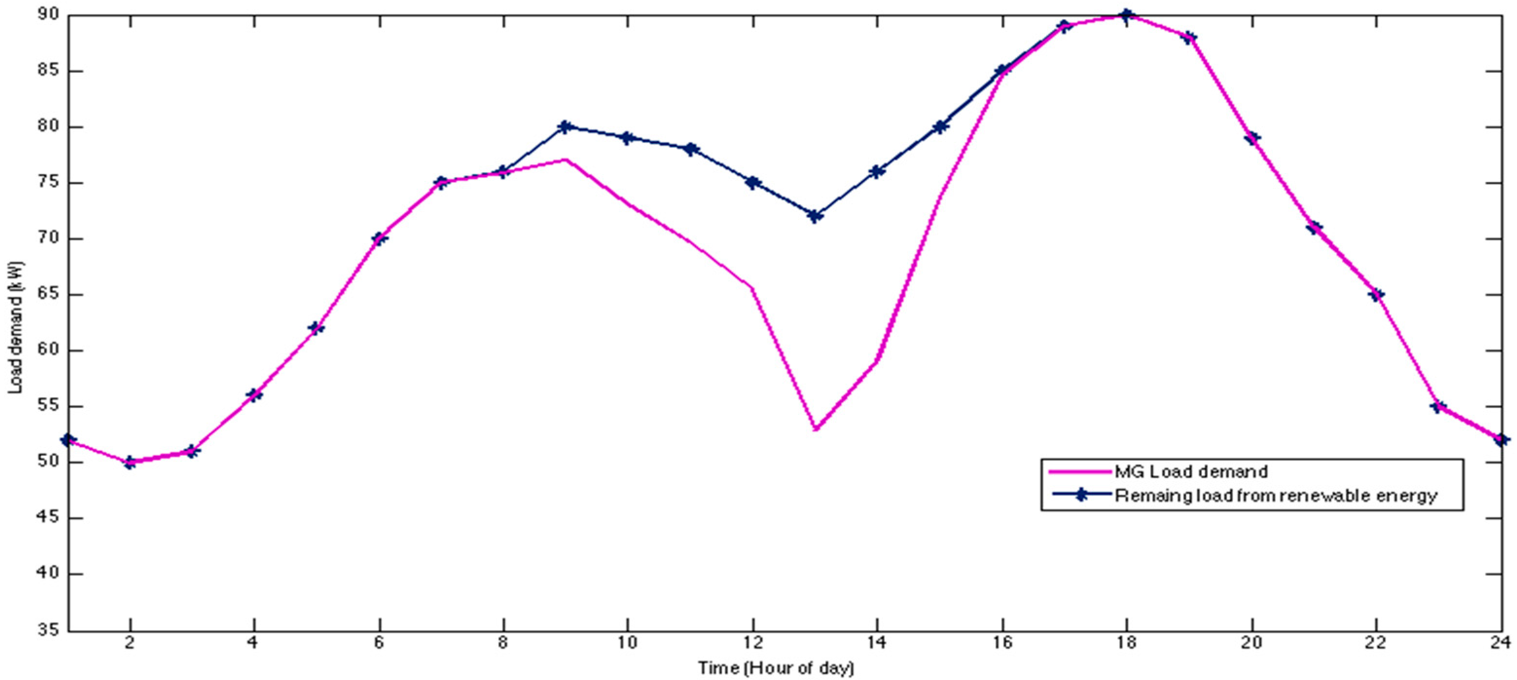
Figure 2 demonstrates the daily energy consumption of the system vs. the load demand after PV generated power subtraction. It is clear from the results that the PV energy production during the daytime can smoothen the load profile, which is beneficial in terms of system cost and emission. The contribution of the remaining DERs will fulfill the MG base load.
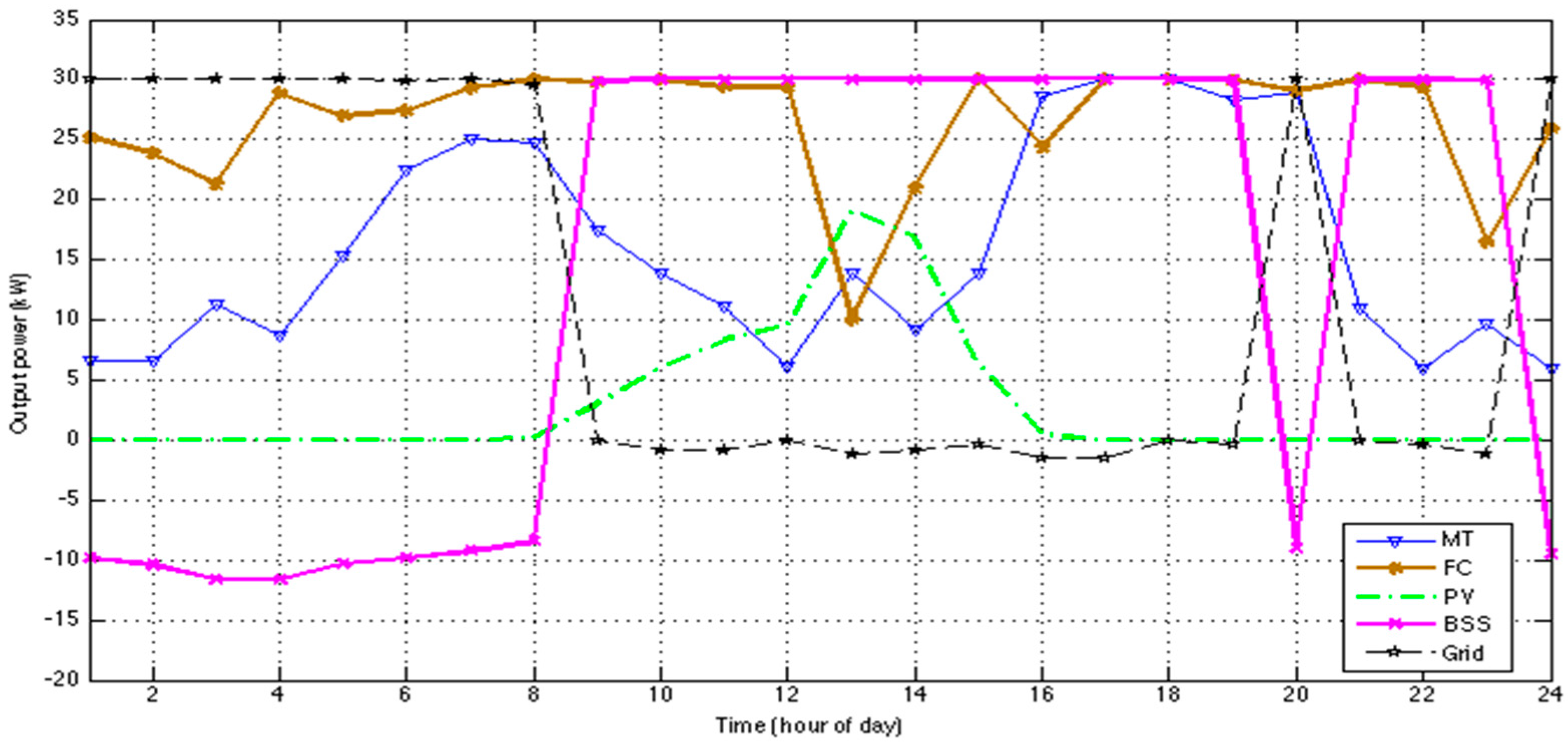
The optimal power outputs of the MG’s DGs, and also the power purchased/sold to the external grid in a typical test day, are shown in Figure 3. As included in the results, the MT and FC are on during the test day to meet the base load. The output of the FC and MT decreases during noontime, and around solar noon, when the PV generation is high. Additionally, there is no need to purchase power from the grid at that time, and there is even some excess generated energy that can be sold to the utility. Since electricity prices are low during the morning and very late at night, it is beneficial for the MG to purchase power from the external grid on its maximum boundary. BSS is in discharging mode when PBSS > 0 and charging mode when PBSS < 0; also, BSS has zero production when PBSS = 0. Thus, the BSS is in charging cycle when the electricity price is low at the beginning of the day, and it is in discharging cycle in the middle of the day when the electricity market price is high, and BSS is required to fulfill some part of the load. The BSS will go back to the initial condition at the end of the day. The optimal operation results in Figure 3 clearly demonstrate that the optimal system behavior and reaction to the various changes such as local power consumption, real-time electricity price, and weather condition.
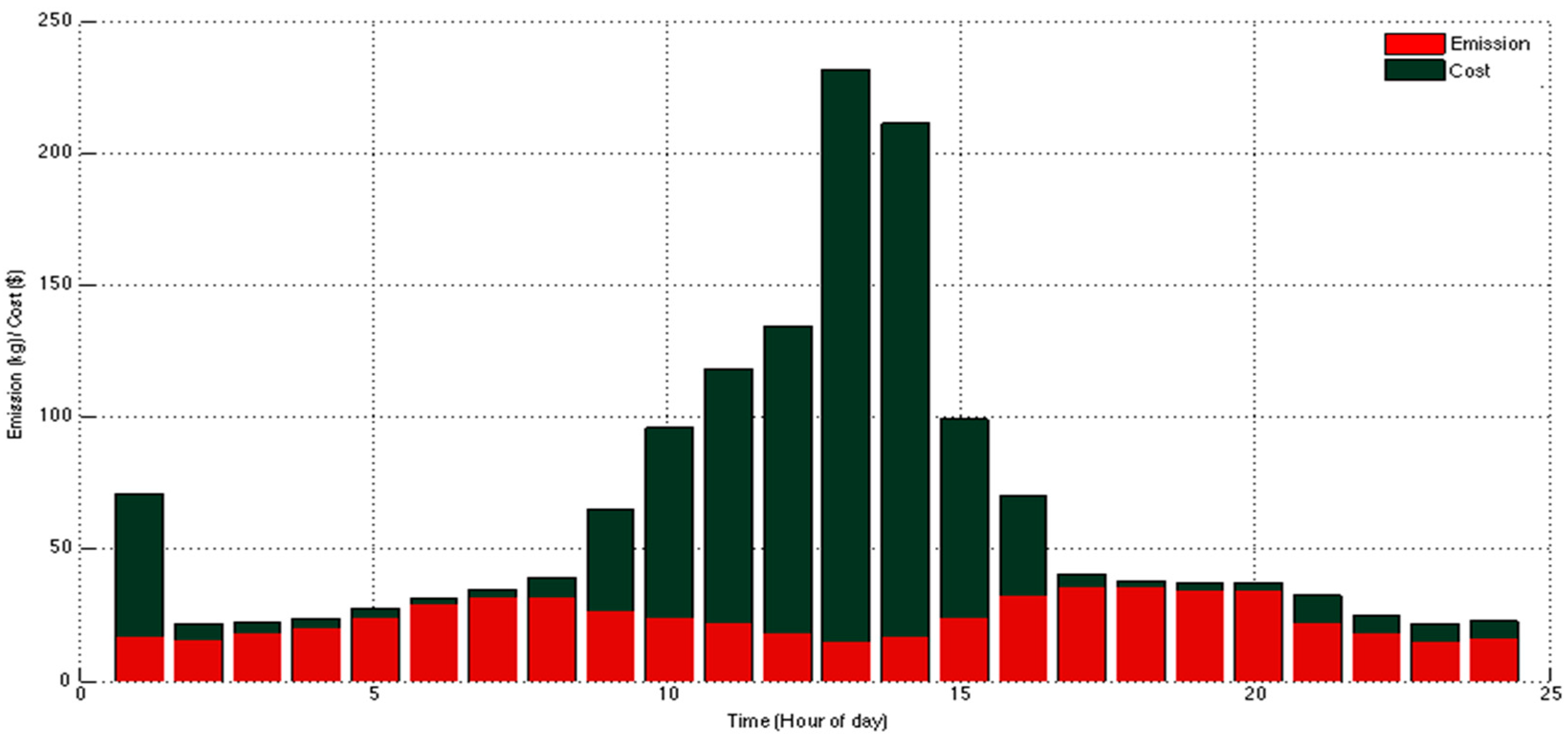
Moreover, net system operation costs and produced emissions are presented in Figure 4. It is concluded from the figure that the system cost has its peak around solar noon, when all of the MG’s DERs are on, and no power is injected from the grid. Although, the amount of generated emission has its off-peak at the same time, because a major part of the load is covered by PV at the mentioned period. In contrast, the MG’s total cost is low at the beginning and end of the day, when the upstream grid meets the majority of the load, and the amount of generated GHGs is on its peak at the same time.
Based on Table 8, a daily system total cost would be $1548.8, and the total generated emission during that day would be 575.6 kg. The optimal results can be compared with the case when the total power demand is purchased from the upstream utility with the electricity price rate, which is presented in Table 5. Also, the generated emission rate in kg per MWh by the utility grid can be extracted from Table 9.
Utilizing all required data, the total operation cost when the whole load demand of the MG is fulfilled by the main grid is calculated and is equal to $2240.6; also, the corresponding generated GHGs emission would be 1584 kg. As it is observed from the results, providing electric energy through the MG utilizing renewable and non-renewable DERs would be a cost-saving option. In addition to the economic benefits, operating a MG that includes renewable resources is an environmentally-friendly choice that would decrease the amount of GHGs in the environment. In this research, the generated emission operating a MG reduced the system emission by one third compared with the conventional power supply.
7. Conclusions
In order to find the solutions of optimally DER operations in a MG, a novel optimization technique has been proposed in this paper, where the modeling goals were minimizing MG operation costs as well as maintenance and emission costs. The mathematical modeling and corresponding constraints of each MG’s components were introduced in order to solve the proposed objective function. Utilizing the presented algorithm along with considering solar PV power generation and electrical load uncertainties, a day-ahead power generation scheduling of DERs was calculated. The contribution of the proposed model focuses on the adjustment of the uncertain parameters inside the approach, which are addressed by utilizing MC simulation in contrast to conventional techniques.
The simulation results have shown that high renewable energy sources penetration will have a significant total effect on the grid operation, especially when emission reduction is one of the system objectives. However, the MG total operation cost rises correspondingly in the investigated time duration. Additionally, the proposed approach can facilitate the choice for the grid-connected MG operator to carry out a stable and economical operation at the planning decision stage for the next day. In consequence, it would be favorable for both system goals when a convenient means of energy exchange was provided between the MG and the upstream utility in the grid-tied mode.
Author Contributions
Hadis Moradi, Amir Abtahi, and Ali Zilouchian conceived and developed the research problem; Hadis Moradi wrote the entire manuscript; Mahdi Esfahanian supervised the paper writing; Amir Abtahi and Ali Zilouchian participated in paper revisions.
Conflicts of Interest
The authors declare no conflict of interest.
References
- Liu, G.; Starke, M.; Xiao, B.; Zhang, X.; Tomsovic, K. Microgrid optimal scheduling with chance-constrained islanding capability. Electr. Power Syst. Res. 2017, 145, 197–206. [Google Scholar] [CrossRef]
- Moradi, H.; De Groff, D.; Abtahi, A. Optimal energy scheduling of a stand-alone multi-sourced microgid considering environmental aspects. In Proceedings of the IEEE Innovative Smart Grid Technologies Conference (ISGT), Arlington, VA, USA, 23–26 April 2017. [Google Scholar]
- Nwulu, N.I.; Xia, X. Optimal dispatch for a microgrid incorporating renewables and demand response. Renew. Energy 2017, 101, 16–28. [Google Scholar] [CrossRef]
- Zhang, Y.; Xie, L.; Ding, Q. Interactive control of coupled microgrids for guaranteed system-wide small signal stability. IEEE Trans. Smart Grid 2016, 7, 1088–1096. [Google Scholar] [CrossRef]
- Frances, A.; Asensi, R.; Garcia, O.; Prieto, R.; Uceda, J. Modeling electronic power converters in smart DC microgrids—An overview. IEEE Trans. Smart Grid 2017, PP, 1. [Google Scholar] [CrossRef]
- Athari, M.H.; Wang, Z. Modeling the uncertainties in renewable generation and smart grid loads for the study of the grid vulnerability. In Proceedings of the IEEE Power & Energy Society Innovative Smart Grid Technologies Conference (ISGT), Minneapolis, MN, USA, 6–9 September 2016; pp. 1–5. [Google Scholar]
- Shahsavari, A.; Fereidunian, A.; Lesani, H. A healer reinforcement approach to smart grid self-healing by redundancy improvement. In Proceedings of the 18th Electric Power Distribution Conference, Kermanshah, Iran, 4 April–1 May 2013; pp. 1–9. [Google Scholar]
- Shin, J.; Lee, J.H.; Realff, M.J. Operational planning and optimal sizing of microgrid considering multi-scale wind uncertainty. Appl. Energy 2017, 195, 616–633. [Google Scholar] [CrossRef]
- Khazaei, H.; Vahidi, B.; Hosseinian, S.H.; Rastegar, H. Two-level decision-making model for a distribution company in day-ahead market. IET Gener. Transm. Distrib. 2015, 9, 308–1315. [Google Scholar] [CrossRef]
- Raoufat, M.E.; Khayatian, A.; Mojallal, A. Performance recovery of voltage source converters with application to grid-connected fuel cell DGs. IEEE Trans. Smart Grid 2016, 99, 1–8. [Google Scholar] [CrossRef]
- Sadeghian, H.R.; Ardehali, M.M. A novel approach for optimal economic dispatch scheduling of integrated combined heat and power systems for maximum economic profit and minimum environmental emissions based on Benders decomposition. Energy 2016, 102, 10–23. [Google Scholar] [CrossRef]
- Hajibandeh, N.; Shafie-khah, M.; Talari, S.; Catalão, P.S.J. The impacts of demand response on the efficiency of energy markets in the presence of wind farms. Technol. Innov. Smart Syst. 2017, 499, 287–296. [Google Scholar]
- Bhattarai, B.P.; Levesque, M.; Bak-Jensen, B.; Pillai, J.; Maier, M.; Tipper, D.; Myers, K. Design and co-simulation of hierarchical architecture for demand response control and coordination. IEEE Trans. Ind. Inform. 2016, 13, 1806–1816. [Google Scholar] [CrossRef]
- Jin, M.; Feng, W.; Liu, P.; Marnay, C.; Spanos, C. MOD-DR: Microgrid optimal dispatch with demand response. Appl. Energy 2017, 187, 758–776. [Google Scholar] [CrossRef]
- Yu, J.; Jing, L.; Haitao, L.; Ming, W.; Yang, L.; Hui, Y. Research on microgrid reconfiguration under rural network fault. In Proceedings of the 2014 International Conference on Power System Technology, Chengdu, China, 20–22 October 2014; pp. 3271–3274. [Google Scholar]
- Mohamed, F.A.; Koivo, H.N. Online management genetic algorithms of microgrid for residential application. Energy Convers. Manag. 2012, 64, 562–568. [Google Scholar] [CrossRef]
- Huang, W.T.; Yao, K.C.; Wu, C.C.; Chang, Y.R.; Lee, Y.D.; Ho, Y.H. A three-stage optimal approach for power system economic dispatch considering microgrids. Energies 2016, 9, 976. [Google Scholar] [CrossRef]
- Su, W.; Wang, J.; Roh, J. Stochastic energy scheduling in microgrids with intermittent renewable energy resources. IEEE Trans. Smart Grid 2014, 5, 1876–1883. [Google Scholar] [CrossRef]
- Liu, C.; Wang, J.; Botterud, A.; Zhou, Y.; Vyas, A. Assessment of impacts of PHEV charging patterns on wind-thermal scheduling by stochastic unit commitment. IEEE Trans. Smart Grid 2012, 3, 675–683. [Google Scholar] [CrossRef]
- Wu, X.; Wang, X.; Qu, C. A hierarchical framework for generation scheduling of microgrids. IEEE Trans. Power Deliv. 2014, 29, 2448–2457. [Google Scholar] [CrossRef]
- Bhattarai, B.; Myers, K.; Bak-Jensen, B.; Paudyal, S. Multi-time scale control of demand flexibility in smart distribution networks. Energies 2017, 10, 37. [Google Scholar] [CrossRef]
- Bhattarai, B.P.; Myers, K.S.; Bush, J.W. Reducing demand charges and onsite generation variability using behind-the-meter energy storage. In Proceedings of the 2016 IEEE Conference on Technologies for Sustainability (SusTech), Phoenix, AZ, USA, 9–11 October 2016; pp. 140–146. [Google Scholar]
- Craparo, E.; Karatas, M.; Singham, D.I. A robust optimization approach to hybrid microgrid operation using ensemble weather forecasts. Appl. Energy 2017, 201, 135–147. [Google Scholar] [CrossRef]
- Maulik, A.; Das, D. Optimal operation of microgrid using four different optimization techniques. Sustain. Energy Technol. Assess. 2017, 21, 100–120. [Google Scholar] [CrossRef]
- Rahmani, R.; Moser, I.; Seyedmahmoudian, M. Multi-agent based operational cost and inconvenience optimization of PV-based microgrid. Sol. Energy 2017, 150, 177–191. [Google Scholar] [CrossRef]
- Dimeas, A.; Hatziargyriou, N. Operation of a multiagent system for microgrid control. IEEE Trans. Power Syst. 2005, 20, 1447–1455. [Google Scholar] [CrossRef]
- Dominguez-Garcia, A.; Hadjicostis, C. Distributed algorithms for control of demand response and distributed energy resources. In Proceedings of the IEEE Conference Decision Control European Control (CDC), Orlando, FL, USA, 12–15 December 2011; pp. 27–32. [Google Scholar]
- Zhang, Y.; Gatsis, N.; Giannakis, G. Robust energy management for microgrids with high-penetration renewables. IEEE Trans. Sustain. Energy 2013, 4, 944–953. [Google Scholar] [CrossRef]
- Wang, Z.; Yang, K.; Wang, X. Privacy-preserving energy scheduling in microgrid systems. IEEE Trans. Smart Grid 2013, 4, 1810–1820. [Google Scholar] [CrossRef]
- Crisostomi, E.; Liu, M.; Raugi, M.; Shorten, R. Plug-and-play distributed algorithms for optimized power generation in a microgrid. IEEE Trans. Smart Grid 2014, 5, 2145–2154. [Google Scholar] [CrossRef]
- Lohri, C.R.; Faraji, A.; Ephata, E.; Rajabu, H.M.; Zubrugg, C. Urban biowaste for solid fuel production: Waste suitability assessment and experimental carbonization in Dar es Salaam, Tanzania. Waste Manag. Res. 2015, 33, 175–182. [Google Scholar] [CrossRef] [PubMed]
- Chiu, H.Y.; Pai, T.Y.; Liu, M.H.; Chang, C.A.; Lo, F.C.; Chang, T.C.; Lo, H.M.; Chiang, C.F.; Chao, K.P.; Lo, W.Y.; et al. Electricity production from municipal solid waste using microbial fuel cells. Waste Manag. Res. 2016, 34, 619–629. [Google Scholar] [CrossRef] [PubMed]
- Anvari Moghaddam, A.; Seifi, A.; Niknam, T. Multi-operation management of a typical micro-grids using particle swarm optimization: A comparative study. Renew. Sustain. Energy Rev. 2012, 16, 1268–1281. [Google Scholar] [CrossRef]
- Soroudi, A.; Aien, M.; Ehsan, M. A probabilistic modeling of photovoltaic modules and wind power generation impact on distribution networks. IEEE Syst. J. 2012, 6, 254–259. [Google Scholar] [CrossRef]
- Aien, M.; Rashidinejad, M.; Fotuhi Firuz-Abad, M. Probabilistic optimal power flow in correlated hybrid wind-PV power systems: A review and a new approach. Renew. Sustain. Energy Rev. 2015, 41, 1437–1446. [Google Scholar] [CrossRef]
- Moradi, H.; Abtahi, A.; Esfahanian, M. Optimal operation of a multi-sourced microgrid to achieve cost and emission targets. In Proceedings of the IEEE Power and Energy Conference at Illinois (PECI), Urbana, IL, USA, 19–20 February 2016; pp. 1–6. [Google Scholar]
- Hawkes, A.D.; Leach, M.A. Modelling high level system design and unit commitment for a microgrid. Appl. Energy 2009, 86, 1253–1265. [Google Scholar] [CrossRef]
- Kerdphol, T.; Fuji, K.; Mitani, Y.; Watanabe, M.; Qudaih, Y. Optimization of a battery energy storage system using particle swarm optimization for stand-alone microgrids. Int. J. Electr. Power Energy Syst. 2016, 81, 32–39. [Google Scholar] [CrossRef]
Figure 1.
Schematic of a grid-connected microgrid with various distributed energy resources (DERs).

Figure 2.
Daily energy consumption before and after renewable energy generation.

Figure 3.
DERs power generation contribution in optimal operation.

Figure 4.
MG operation cost vs. generated emission over 24 h.


Table 1.
Percentage values of PV arrays rated power used in the system.
| Hour | PV Usage Percentage | Hour | PV Usage Percentage |
|---|---|---|---|
| 1 | 0 | 13 | 0.7648 |
| 2 | 0 | 14 | 0.6736 |
| 3 | 0 | 15 | 0.252 |
| 4 | 0 | 16 | 0.1352 |
| 5 | 0 | 17 | 0.0176 |
| 6 | 0 | 18 | 0 |
| 7 | 0 | 19 | 0 |
| 8 | 0.0064 | 20 | 0 |
| 9 | 0.12 | 21 | 0 |
| 10 | 0.2408 | 22 | 0 |
| 11 | 0.3344 | 23 | 0 |
| 12 | 0.3824 | 24 | 0 |
Table 2.
Average MG hourly load demand.
| Hour | Load Value (kW) | Hour | Load Value (kW) |
|---|---|---|---|
| 1 | 52.2 | 13 | 72.0 |
| 2 | 50.5 | 14 | 76.8 |
| 3 | 51.0 | 15 | 80.6 |
| 4 | 56.9 | 16 | 85.2 |
| 5 | 62.4 | 17 | 89.1 |
| 6 | 70.1 | 18 | 90.3 |
| 7 | 75.9 | 19 | 88.7 |
| 8 | 76.8 | 20 | 79.9 |
| 9 | 80.7 | 21 | 71.8 |
| 10 | 79.3 | 22 | 65.2 |
| 11 | 78.7 | 23 | 55.7 |
| 12 | 75.1 | 24 | 52.5 |
Table 3.
Installed distributed energy resources in the MG.
| DER Type | Min Power (kW) | Max Power (kW) |
|---|---|---|
| Solar PV | 0 | 26 |
| Micro-gas Turbine | 6 | 36 |
| Fuel Cell | 3 | 32 |
| Battery Storage | −30 | 30 |
| Utility | −30 | 30 |
Table 4.
Operation costs of DER units.
| Type | Power Generation Cost ($/kWh) | O&M Cost ($/kWh) | Start-Up/Shut-Down Cost ($) |
|---|---|---|---|
| MT | 0.457 | 0.457 | 0.96 |
| FC | 0.294 | 0.08618 | 1.65 |
| BSS | 0.23 | 0 | 0 |
| PV | 2.584 | 0.2082 | 0 |
Table 5.
Real-time market energy prices.
| Hour | Electricity Price ($/kWh) | Hour | Electricity Price ($/kWh) |
|---|---|---|---|
| 1 | 0.125 | 13 | 2.000 |
| 2 | 0.115 | 14 | 0.750 |
| 3 | 0.100 | 15 | 2.000 |
| 4 | 0.100 | 16 | 1.000 |
| 5 | 0.115 | 17 | 0.900 |
| 6 | 0.125 | 18 | 0.300 |
| 7 | 0.140 | 19 | 0.200 |
| 8 | 0.175 | 20 | 0.150 |
| 9 | 0.400 | 21 | 0.200 |
| 10 | 0.750 | 22 | 0.620 |
| 11 | 2.000 | 23 | 0.300 |
| 12 | 2.000 | 24 | 0.125 |
Table 6.
DERs generated emission.
| Type | CO2 (kg/MWh) | SO2 (kg/MWh) | NOx (kg/MWh) |
|---|---|---|---|
| MT | 720 | 0.0036 | 0.1 |
| FC | 460 | 0.003 | 0.0075 |
| BSS | 10 | 0.0002 | 0.001 |
| PV | 0 | 0 | 0 |
Table 7.
Day-ahead energy scheduling of MG components.
| Distributed Generation Units Outputs (kW) | |||||
|---|---|---|---|---|---|
| Hour | MT | FC | PV | BSS | Main Grid |
| 1 | 6.6683 | 25.1718 | 0 | −9.8402 | 30.0000 |
| 2 | 6.5543 | 23.8462 | 0 | −10.3994 | 30.0000 |
| 3 | 11.3806 | 21.2822 | 0 | −11.6693 | 29.9971 |
| 4 | 8.7803 | 28.8892 | 0 | −11.6693 | 30.0000 |
| 5 | 15.4236 | 26.9856 | 0 | −10.3394 | 30.0000 |
| 6 | 22.4248 | 27.4312 | 0 | −9.8402 | 29.9838 |
| 7 | 24.9745 | 29.2703 | 0 | −9.2454 | 29.9992 |
| 8 | 24.7234 | 29.9999 | 0.1604 | −8.4458 | 29.5628 |
| 9 | 17.3756 | 29.7481 | 3.0030 | 29.8832 | −0.0072 |
| 10 | 13.8661 | 30.0000 | 6.0210 | 30.0000 | −0.8867 |
| 11 | 11.0968 | 29.4063 | 8.3602 | 30.0000 | −0.8643 |
| 12 | 6.1000 | 29.4108 | 9.5600 | 30.0000 | 0 |
| 13 | 13.9605 | 10.0509 | 19.1204 | 30.0000 | −1.1315 |
| 14 | 9.1257 | 20.9291 | 16.8402 | 29.9999 | −0.8944 |
| 15 | 13.9663 | 29.9998 | 6.3002 | 29.9998 | −0.2661 |
| 16 | 28.6901 | 24.3317 | 0.4401 | 30.0000 | −1.4018 |
| 17 | 30.0000 | 30.0000 | 0 | 30.0000 | −1.4400 |
| 18 | 30.0000 | 30.0000 | 0 | 30.0000 | 0 |
| 19 | 28.3492 | 29.9504 | 0 | 29.9962 | −0.2953 |
| 20 | 28.9221 | 29.0329 | 0 | −8.9545 | 29.9998 |
| 21 | 10.9166 | 30.0000 | 0 | 30.0000 | 0 |
| 22 | 6.0333 | 29.3473 | 0 | 29.9994 | −0.3787 |
| 23 | 9.7418 | 16.4747 | 0 | 29.9687 | −1.1853 |
| 24 | 6.0000 | 25.8402 | 0 | −9.5402 | 30.0000 |
Table 8.
Total system cost and generated emission in each hour.
| Hour | Hourly Cost/Emission | Hour | Hourly Cost/Emission | ||
|---|---|---|---|---|---|
| Cost | Emission | Cost | Emission | ||
| 1 | 70.8115 | 16.4796 | 13 | 231.2587 | 14.9766 |
| 2 | 21.6447 | 15.7924 | 14 | 210.6758 | 16.4992 |
| 3 | 22.1378 | 18.1092 | 15 | 99.1108 | 24.1575 |
| 4 | 23.7214 | 19.7288 | 16 | 69.9885 | 32.1528 |
| 5 | 27.2846 | 23.6173 | 17 | 40.1758 | 35.7033 |
| 6 | 31.6332 | 28.8652 | 18 | 37.8535 | 35.7036 |
| 7 | 34.6445 | 31.5423 | 19 | 36.9007 | 34.4918 |
| 8 | 38.8966 | 31.6878 | 20 | 37.2314 | 34.2719 |
| 9 | 64.9007 | 26.4955 | 21 | 32.3031 | 21.9616 |
| 10 | 95.6678 | 24.0858 | 22 | 25.1153 | 18.1447 |
| 11 | 118.1412 | 21.8184 | 23 | 21.8267 | 14.8934 |
| 12 | 134.0407 | 18.1500 | 24 | 22.7936 | 16.3058 |
Table 9.
Utility grid emission production rate per MWh.
| Type | CO2 (kg/MWh) | SO2 (kg/MWh) | NOx (kg/MWh) |
|---|---|---|---|
| Utility grid | 923 | 3.584 | 2.296 |
© 2017 by the authors. Licensee MDPI, Basel, Switzerland. This article is an open access article distributed under the terms and conditions of the Creative Commons Attribution (CC BY) license (http://creativecommons.org/licenses/by/4.0/).
Share and Cite
MDPI and ACS Style
Moradi, H.; Esfahanian, M.; Abtahi, A.; Zilouchian, A. Modeling a Hybrid Microgrid Using Probabilistic Reconfiguration under System Uncertainties. Energies 2017, 10, 1430. https://doi.org/10.3390/en10091430
AMA Style
Moradi H, Esfahanian M, Abtahi A, Zilouchian A. Modeling a Hybrid Microgrid Using Probabilistic Reconfiguration under System Uncertainties. Energies. 2017; 10(9):1430. https://doi.org/10.3390/en10091430
Chicago/Turabian StyleMoradi, Hadis, Mahdi Esfahanian, Amir Abtahi, and Ali Zilouchian. 2017. "Modeling a Hybrid Microgrid Using Probabilistic Reconfiguration under System Uncertainties" Energies 10, no. 9: 1430. https://doi.org/10.3390/en10091430
Note that from the first issue of 2016, this journal uses article numbers instead of page numbers. See further details here.