Generic Type 3 Wind Turbine Model Based on IEC 61400-27-1: Parameter Analysis and Transient Response under Voltage Dips

Abstract

This paper analyzes the response under voltage dips of a Type 3 wind turbine topology based on IEC 61400-27-1. The evolution of both active power and rotational speed is discussed in detail when some of the most relevant control parameters, included in the mechanical, active power and pitch control models, are modified. Extensive results are also included to explore the influence of these parameters on the model dynamic response. This work thus provides an extensive analysis of the generic Type 3 wind turbine model and provides an estimation of parameters not previously discussed in the specific literature. Indeed, the International Standard IEC 61400-27-1, recently published in February 2015, defines these generic dynamic simulation models for wind turbines, but does not provide values for the parameters to simulate the response of these models. Thus, there is a pressing need to establish correlations between IEC generic models and specific wind turbine manufacturer models to estimate suitable parameters for simulation purposes. Extensive results and simulations are also included in the paper.

1. Introduction

During the last decade, the integration of renewables into power systems has increased considerably, mainly due to successful policies and substantial investments. Indeed, according to [1], renewables are essential to achieve long-term climate targets; reaching a 30% share by 2030 should be sufficient to prevent global temperatures from rising more than 2 ${}^{\circ }$C above pre-industrial levels. Currently, of the different technologies, wind and solar Photovoltaics (PV) are, globally, the fastest-growing sources of electricity and offer technologically-mature and economically-affordable solutions [2]. In this scenario, the International Energy Agency (IEA) roadmap targets a 15–18% share of global electricity from wind power by 2050, a notable increase of the 12% aimed for in 2009 [3]. This increasing share of wind power has created the need for wind turbine (WT) and wind power plant (WPP) models to be used in power system stability analysis. However, conventional electromagnetic transients simulation (EMTS) models proposed by wind turbine manufacturers fail to satisfy the current needs demanded by Transmission System Operators (TSO) for these power system stability analyses; mainly due to the models being complex, highly detailed and generally confidential. In fact, these manufacturer models usually simulate the behavior of all of the internal components of the wind turbine, and hence, a large number of parameters is required to achieve accurate simulations, as well as high computational time costs or even specific software for their simulations [4,5]. Therefore, it would be desirable to propose efficient and flexible simulation models that respond to TSO requirements [5,6].

To solve this issue, international institutions worldwide are developing new generic models, also known as standard or simplified models, defined by a limited number of parameters [7,8]. These models are available for any specific simulation software to simulate wind turbines integrated in the grid. The International Electrotechnical Commission published the first version of the Standard IEC 61400-27-1 [9] in February 2015, where these generic wind turbine models were initially defined. This standard classifies the different topologies of wind turbines into four types, representing the majority of wind turbines installed in power systems. The four types of wind turbine generators, which are mainly differentiated by the generator, are: (Type 1) wind turbines equipped with an asynchronous generator directly connected to the grid (usually squirrel-cage) [10]; (Type 2) wind turbines equipped with an asynchronous generator with a variable rotor resistance, directly connected to the grid; (Type 3) wind turbines equipped with a Doubly-Fed Induction Generator (DFIG), with the stator directly connected to the grid and the rotor connected through a back-to-back power converter; (Type 4) wind turbines connected to the grid through a Full-Scale power Converter (FSC) [11].

These dynamic models are suitable to be tested even under transients, such as switching of power lines, loss of generation or loads, balanced faults, voltage dips, etc. [12,13]. In this work, the generic Type 3 WT model facing a three-phase voltage dip will be tested. These balanced faults are not the most common, but they represent the worst-case dimensional scenario. However, the study of unbalanced faults also constitutes a very interesting case for DFIG and FSC wind turbines (Types 3 and 4, respectively), but currently, the wind turbine models specified in IEC 61400-27-1 are only for fundamental frequency positive sequence response. In [14], field measurements from a 52-MW wind power plant are used to validate an IEC Type 3 wind turbine model with a wind turbine level voltage controller and with a wind power plant level power factor controller. Nevertheless, in the specific literature, there are few studies on the values of parameters to be used for simulation purposes [15,16]. Moreover, the recent publication of the standard, as well as the constraints of the wind turbine manufacturers [17] have led to the need to conduct studies that provide parameter values and simulation results [18], thus allowing the adjustment of the generic wind turbine and wind power plant models by both researchers and institutions [19,20]. Finally, the contributions of the authors presented in the present work may be considered by the International Electrotechnical Commission for inclusion in Edition 2 of IEC 61400-27-1, which is currently under development and is intended for publication in 2018.

Considering previous works and current TSO requirements, this paper describes a generic Type 3 wind turbine model developed in MATLAB/Simulink based on the IEC 61400-27-1 standard. The parameters of the model have been estimated to provide a dynamic response under voltage dips. Additionally, the results have been compared to those of other studies and simulations by manufacturers [21,22,23]. Extensive simulations have been conducted, modifying the parameters and discussing their effects on the wind turbine response in terms of active power and rotational speed. The contributions of the current paper focus on: (i) providing public parameter values and simulation results of a generic Type 3 wind turbine model; (ii) analyzing the influence of the parameter variations on the dynamic wind turbine response under voltage dips and describing the process of model tuning; (iii) contributing to the development of Edition 2 of IEC 61400-27-1.

The rest of the paper is structured as follows: Section 2 introduces the main characteristics of the DFIG wind turbine topology, the details of its implementation in MATLAB/Simulink and describes the methodology. Section 3 discusses the simulation results related to the mechanical two-mass model, and the influence of the control system parameters is studied in Section 4. Section 5 analyzes the effects of varying the parameters of voltage dips on the model’s response. Finally, Section 6 presents conclusions.

2. IEC 61400-27-1 Type 3 Wind Turbine Model

According to the classification presented in the previous section, Type 3 is currently the most widely-used topology. Indeed, around 45% of the wind turbines installed in Europe are of this type [24]. Type 4 wind turbines are increasingly being integrated into new wind power plants, mainly due to their control and stability advantages. as well as the reduction in electronic component cost. Thus, both types of WTs constitute an interesting field of study. In this sense, due to the benefits of using a full power converter, from the TSO point of view, the performance of Type 4 is simpler than Type 3. In fact, the standard Type 4 WT model can be considered a simplified Type 3 model. Consequently, this paper focuses on a Type 3 wind turbine generic model from a more general perspective.

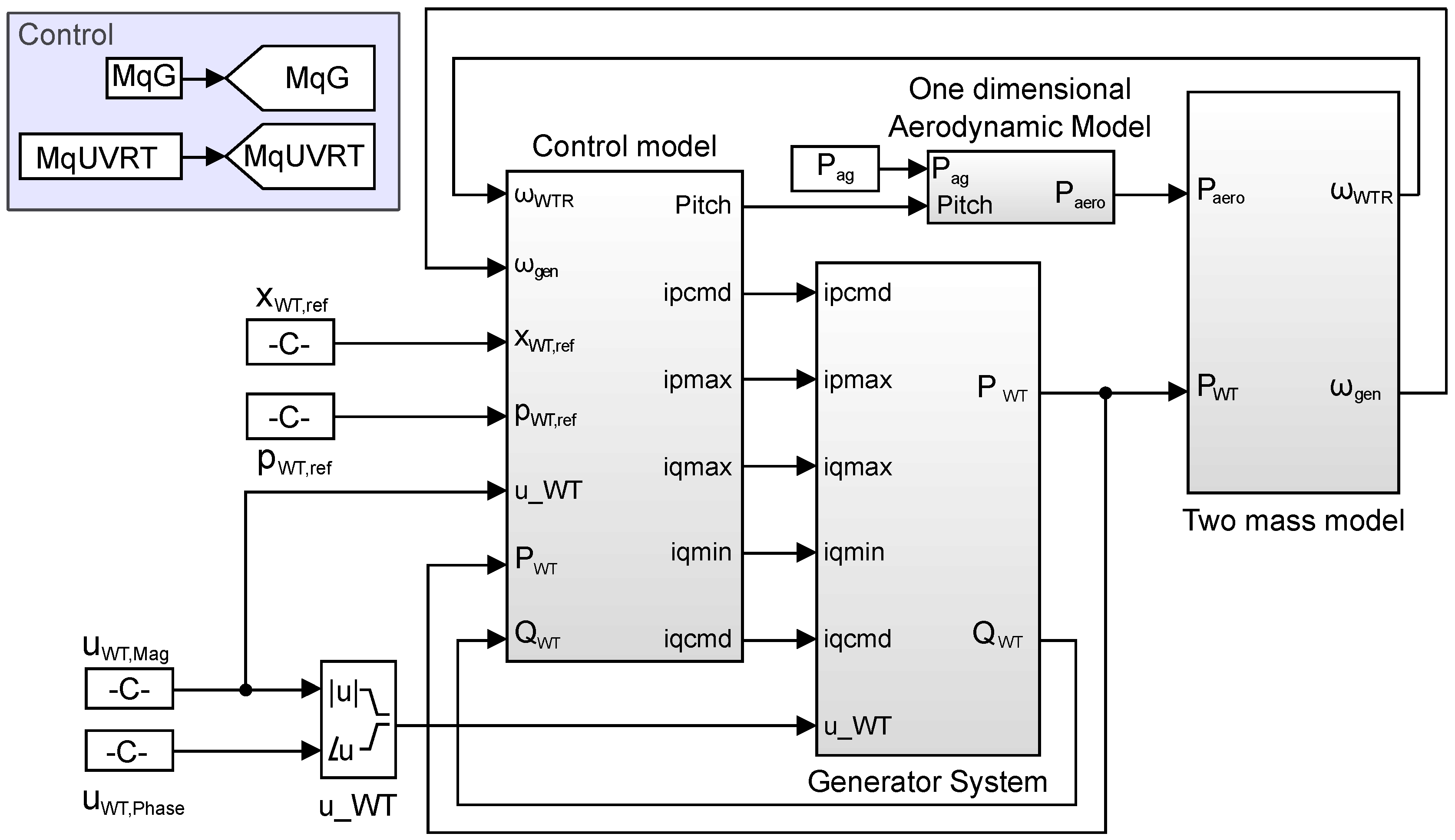
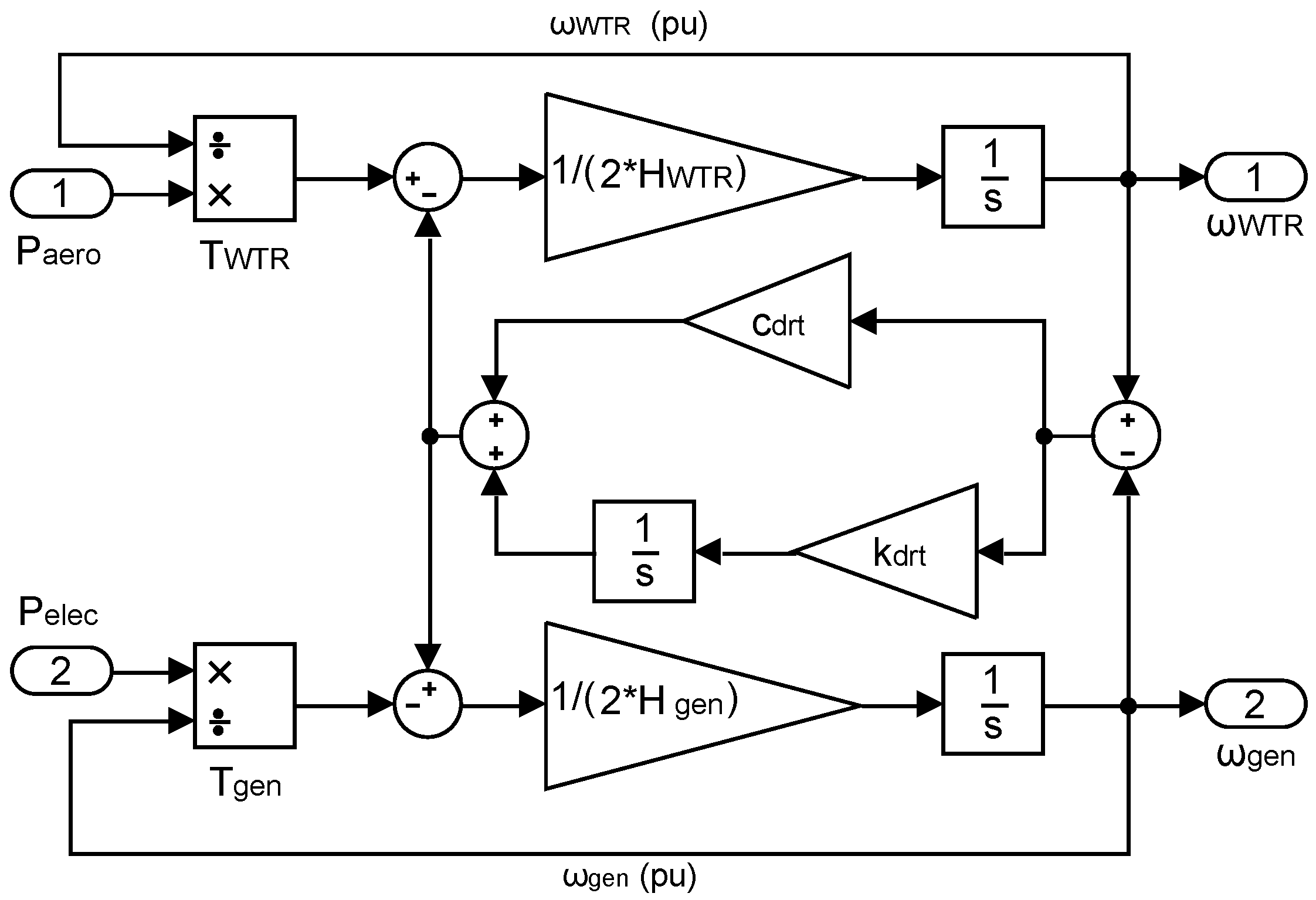
2.1. MATLAB/Simulink Implementation of the Type 3 WT Model

Figure 1 shows the general structure of the generic Type 3 WT model implemented in MATLAB/Simulink (The MathWorks, Inc, Natick, MA, USA). This model has been developed following the guidelines provided by IEC 61400-27-1 [9] and represents one of the first implementations in MATLAB/Simulink in the scientific literature. The dynamic performance depends on both active and reactive power references, $p_{WT,ref}$ and $x_{WT,ref}$, respectively, as well as two further control parameters setting the reactive power control mode $\left(MqG\right)$ and the response under voltage dips $\left(MqUVRT\right)$. A two-mass model is used to simulate the mechanical interactions between high and low speed shafts. The wind turbine rotor (along with the blades) and the electrical generator are modeled by their inertia parameters. They are coupled by a spring with a certain stiffness and a damper with a damping coefficient. These parameters have a significant effect on the active power $\left(P_{WT}\right)$ and generator rotational speed $\left({\omega }_{WTR}\right)$. Further information can be found in Section 3.

With regard to the electrical generator model, Type 1 and Type 2 use an electrical generator model derived from the simulation software. However, and in line with IEC 61400-27-1, the generic Type 3 model is composed of a conventional block diagram. The voltage input is considered as a balanced three-phase voltage input, defined by both magnitude and phase, instead of using a three-phase source, as can be seen in the lower left side of Figure 1 $\left(u_{WT,Mag}\mathrm{and}{u}_{WT,Phase}\right)$

The electrical generator system is a simplification based on [25,26], including the power converter dynamics; see Figure 2. It is mainly commanded by an active and a reactive current signal provided by the control system. Moreover, the corresponding IEC Standard divides the Type 3 generic model into two types depending on the Fault Ride-Through (FRT) solution adopted [5]: (i) Type 3A, with no protection system to avoid the disconnection of the wind turbine under voltage dips [27]; (ii) Type 3B, including a crowbar protection system to avoid over-currents under voltage dips, thus preventing power converter damage. In the generic Type 3B model, this crowbar system multiplies the current references of the generator by zero for a certain period of time, when the variation of the voltage goes beyond a certain limit [18]. Taking into account that this protection system is commonly used by wind turbine manufacturers to meet the mandatory grid codes in Europe [28], the model implemented in this paper is Type 3B.

Figure 3 shows the control system, also included in Figure 1. The control system of the generic Type 3 WT model does not represent the actual controller of the WT, which sets the references to the Rotor-Side Converter (RSC) and the Grid-Side Converter (GSC), but provides the current command signals to obtain an accurate response of active and reactive power, observed from the grid side. This control system is composed of five control subsystems. Active power and pitch control systems are discussed in detail due to their influence on $P_{WT}$ and ${\omega }_{WTR}$, which are the main variables analyzed in this work. The reactive power control system (Q control) provides the reactive current reference $\left(i_{qcmd}\right)$, used as an input to the electrical generator system according to reference $x_{WT,ref}$ and the reactive power control mode (voltage control, reactive power control or power factor control). Both the current and reactive power limitation control subsystems set the maximum and minimum currents and reactive power values that the wind turbine is able to provide, according to parameters such as voltage or active power.

Finally, the influence of the pitch blade angle on the wind power absorbed by the wind turbine is modeled by the aerodynamic model; see Figure 4. It is a one-dimensional model where $P_{ag}$ is the active wind power (in pu) modeled by a constant parameter ($P_{ag}$ in Figure 1). This parameter, in accordance with IEC 61400-27-1 [9], is kept constant during the simulation.

2.2. Simulations Conducted for the Parameter and Transient Response Analysis

This paper aims to analyze the active power $\left(P_{WT}\right)$ and the rotational speed of the wind turbine rotor $\left({\omega }_{WTR}\right)$ submitted to voltage dips when the IEC 61400-27-1 Type 3 model parameters are modified. Specifically, the mechanical two-mass model and the active power control and the pitch control systems have been modified, and their corresponding responses have been analyzed. Parameter values and variations are summarized in

Table 1. Parameter values of Type 3 WT: references and variations.

System	Parameter	Ref. Value	Var.Range
Two mass model	$H_{WTR}$-Inertia constant of WT rotor (s)	10	$\left[51025\right]$
	$H_{gen}$-Inertia constant of generator (s)	1	$\left[0.313\right]$
	$k_{drt}$-Drive train stiffness (pu)	100	$\left[20100500\right]$
	$c_{drt}$-Drive train damping (pu)	0.5	$\left[0.20.51\right]$
Active power control	$K{P}_P$-PI controller proportional gain	6	$\left[0.5610\right]$
	$K{I}_P$-PI controller integration parameter	3	$\left[0.3324\right]$
	$K_{DTD}$-Gain for active drive train damping	0.5	$\left[00.53\right]$
Pitch control	$K{I}_{\omega }$-Speed PI controller integration gain	50	$\left[1050500\right]$
	$K{P}_{\omega }$-Speed PI controller proportional gain	200	-
	$K{I}_c$-Power PI controller integration gain	10	$\left[11040\right]$
	$K{P}_c$-Power PI controller proportional gain	10	-
	$K{P}_X$-Pitch cross coupling gain	0	$\left[00.1\right]$

. A reference value for each parameter has been defined in order to obtain a benchmark system. Subsequently, each parameter can be set to a lower and a higher value than the corresponding reference. The Type 3 WT model’s responses under voltage dips for the different parameter values are depicted in the same axis to compare the influence of these variations on the active power and rotational speed evolution along the transient. The values of these parameters do not follow a physically-based pattern. They have been selected to clearly represent different performances in order to provide guidelines for Type 3 model adjustment under certain simulation conditions. For example, conventional values of $H_{WTR}$ are usually from 5 s to 15 s.

The simulations carried out by the authors are based on a balanced three-phase voltage dip, with a duration of 0.2 s and a residual voltage of 0.1 pu. This voltage dip has been considered in order to follow the guidelines provided by IEC 61400-21 [29], which consider a three-phase voltage dip with a residual voltage of $0.2\pm 0.05\mathrm{pu}$ with a duration of 0.2 s. Moreover, the voltage dip considered is more severe than this reference in order to be included within the guidelines of the recently-published Commission Regulation (EU) 2016/631 [28], which considers the minimum voltage of 0.05–0.30 pu with a duration of 0.14–0.25 s for the most restrictive conditions.

Steady-state conditions are considered before these transients. An additional 1-s time interval before the dip is also shown in the simulations to represent the previous steady-state values. As a preliminary finding, the benchmark response of the initial system values is shown in Figure 5. This response represents the dynamic response of the Type 3 WT model under the voltage dip. Parameters from the initial benchmark system have been adjusted to be in line with the results published in previous works [18,22].

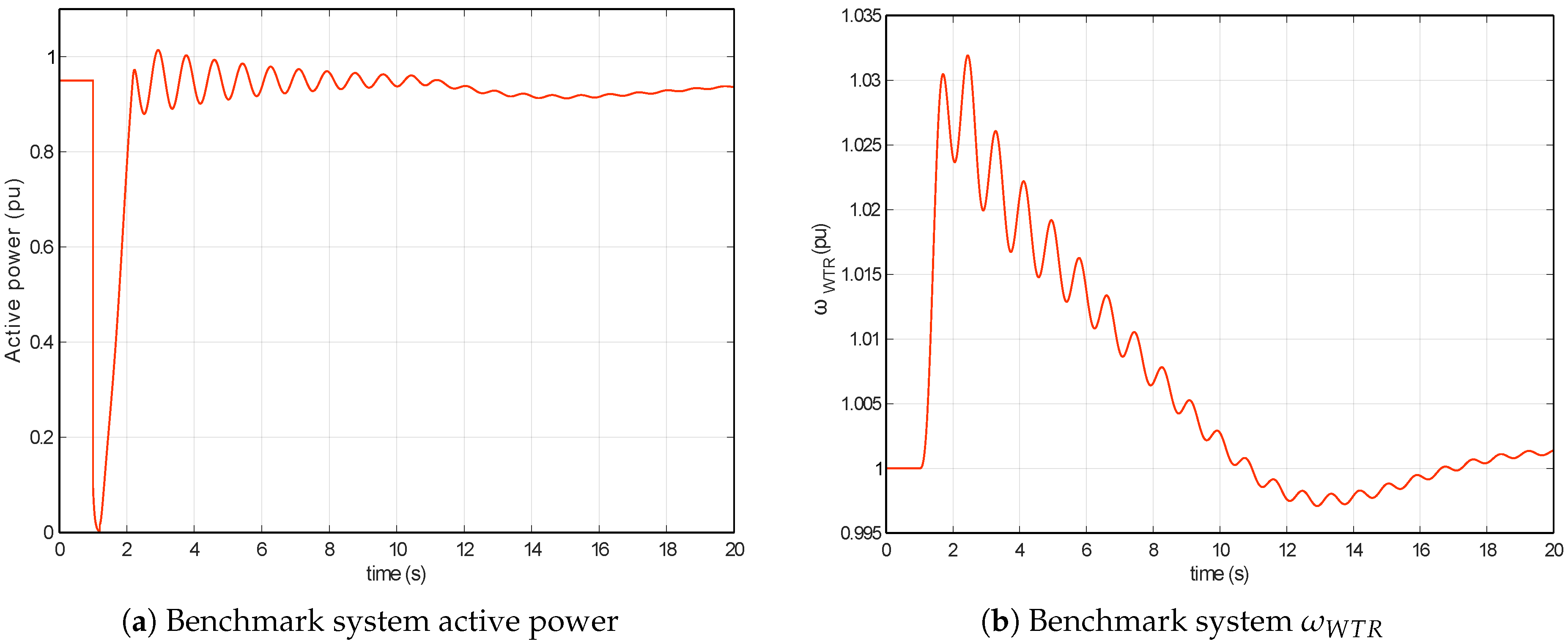
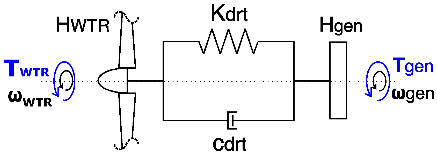
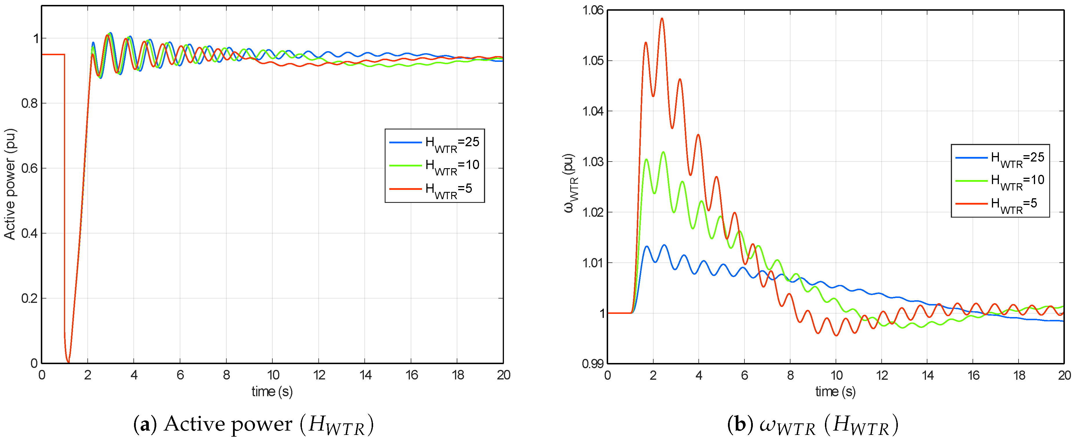
3. Mechanical Parameter Analysis under Voltage Dips of the Type 3 WT Model

Standard IEC 61400-27-1 establishes a mechanical two mass model to simulate the interaction between high and low speed shafts [30]. Both shafts are coupled by a spring with a certain stiffness $\left(k_{drt}\right)$ and a damper with a certain damping coefficient $\left(c_{drt}\right)$. The wind turbine rotor and the electrical generator are represented by their inertia coefficients $\left(H_{WTR}and{H}_{gen},\mathrm{respectively}\right)$. A representation of this relationship is shown in Figure 6. Both shafts rotate with a certain speed $\left({\omega }_{WTR}and{\omega }_{gen}\right)$ and are subjected to a torque. The wind turbine rotor torque $\left(T_{WTR}\right)$ represents the mechanical aerodynamic torque of the wind. The electrical generator torque $\left(T_{gen}\right)$ represents the electromagnetic torque. The expressions to describe system performance are the following [31]:

$$2H_{WTR}·{\displaystyle \frac{d{\omega }_{WTR}}{dt}}=T_{WTR}-k_{drt}·({\theta }_{gen}-{\theta }_{WTR})-c_{drt}·({\omega }_{WTR}-{\omega }_{gen}),$$

(1)

$$2H_{gen}·{\displaystyle \frac{d{\omega }_{gen}}{dt}}=-T_{gen}+k_{drt}·({\theta }_{gen}-{\theta }_{WTR})+c_{drt}·({\omega }_{WTR}-{\omega }_{gen}).$$

(2)

Figure 7 shows the mechanical system implemented in MATLAB/Simulink. Mechanical wind power $\left(P_{aero}={\omega }_{WTR}·T_{WTR}\right)$ obtained from the aerodynamic model and electrical active power $\left(P_{elec}={\omega }_{gen}·T_{gen}\right)$ obtained from the generator system are considered as the inputs of the system. The variation of the four parameters that define this system ($H_{WTR},H_{gen},k_{drt}$ and $c_{drt}$) modifies the response of the overall system in terms of $P_{WT}$ and ${\omega }_{WTR}$ response. Subsequently, the influence of these parameter variations on the Type 3 WT response under voltage dips is analyzed during the transient, considering the parameter values given in Table 1.

Figure 8 shows the $P_{WT}$ and ${\omega }_{WTR}$ dynamic response under a voltage dip when $H_{WTR}$ is modified according to Table 1. $H_{WTR}$ variations do not have a significant influence on the active power response (see Figure 8a), reducing the oscillation frequency and the over-response before the new steady-state conditions. As can be seen in Figure 8b, ${\omega }_{WTR}$ oscillations are clearly affected by the $H_{WTR}$ parameter variation, presenting an inverse relation with ${\omega }_{WTR}$ frequency and oscillations.

The transient response of the system when the $H_{gen}$ parameter is modified is shown in Figure 9. The increase in this parameter makes a considerable contribution to the oscillations of both $P_{WT}$ and ${\omega }_{WTR}$; see Figure 9a,b. The oscillation frequency is inversely proportional to the value of $H_{gen}$. However, the oscillation amplitude proportionally increases with the $H_{gen}$ parameter value. This increasing $H_{gen}$ also has an effect that is inversely proportional to the oscillation damping.

The frequency of these oscillations $\left({\omega }_{osc}\right)$ can be determined by the following expression [32],

$${\omega }_{osc}=\sqrt{k_{drt}·\left({\displaystyle \frac{1}{2·H_{WTR}}}+{\displaystyle \frac{1}{2·H_{gen}}}\right)}.$$

(3)

An interval from 1-5 Hz produces usual values for commercial Type 3 wind turbines. These oscillations are proportional to $k_{drt}$ values and inversely proportional to both $H_{WTR}$ and $H_{gen}$ parameters. However, and considering that the value of $H_{WTR}$ is usually much higher than one, its influence can be considered as almost negligible; see Figure 8. In contrast, $H_{gen}$ variations clearly have a notable influence on the transient response, as shown in Figure 9.

According to Equation (3), the increase in the spring’s stiffness ($k_{drt}$) proportionally affects the frequency of the response oscillations; see Figure 10. This parameter has an important influence on the active power oscillation amplitude (Figure 10a). Moreover, the $k_{drt}$ parameter has a much greater effect than any other parameter under voltage dips. The ${\omega }_{WTR}$ oscillation amplitude is lower than $k_{drt}$ variations, in an inverse relation with the increasing $H_{gen}$ (Figure 10b). Finally, the damping coefficient variations ($c_{drt}$) have no influence on the oscillations, beyond the rate at which they are damped. Figure 11 shows the active power and rotational speed responses under $c_{drt}$ variations. The $c_{drt}$ parameter can be artificially increased in wind turbines to emulate active damping performed by real control by means of this ‘passive damping coefficient’ [33].

4. Control Parameter Analysis under Voltage Dips of the Type 3 WT Model

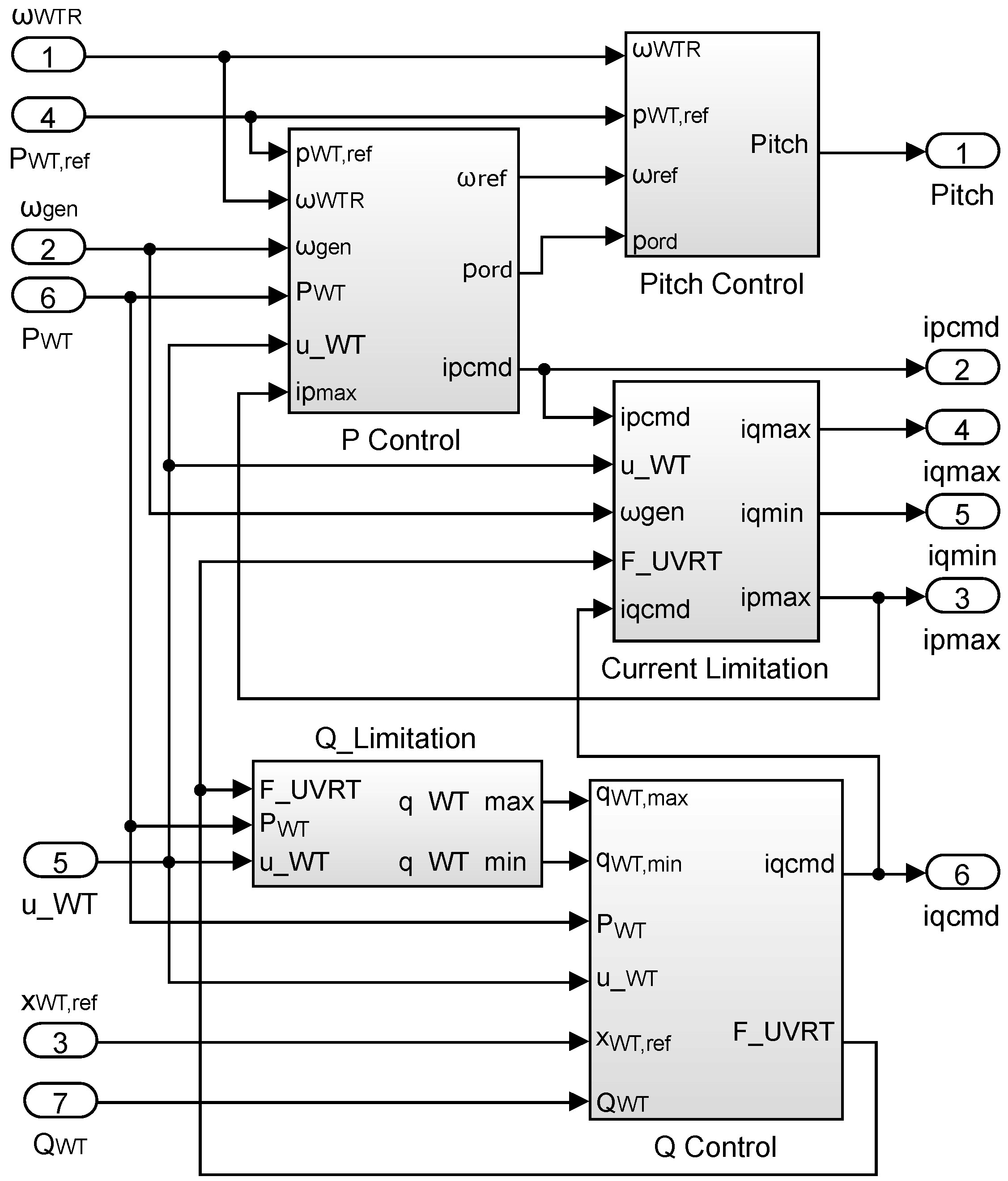
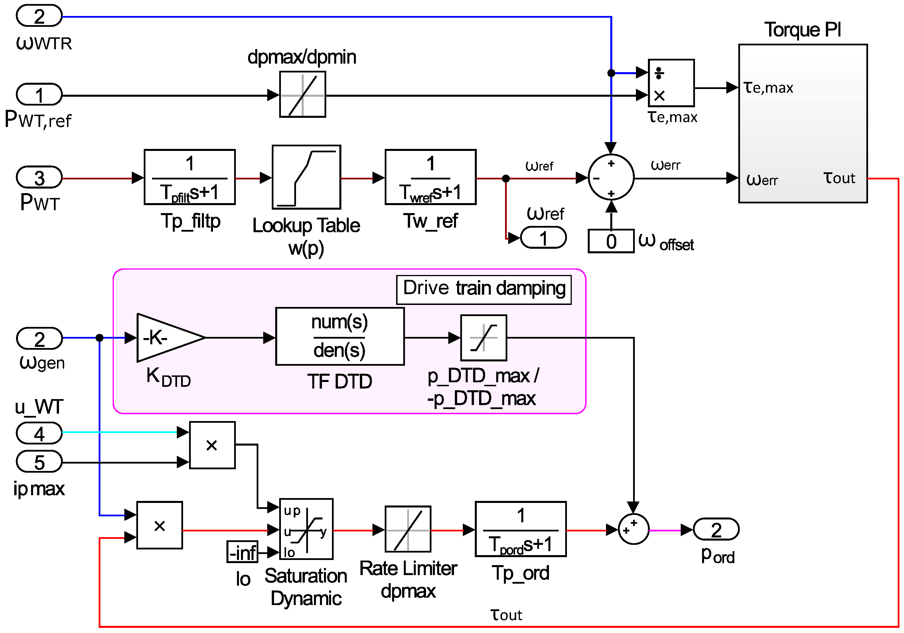
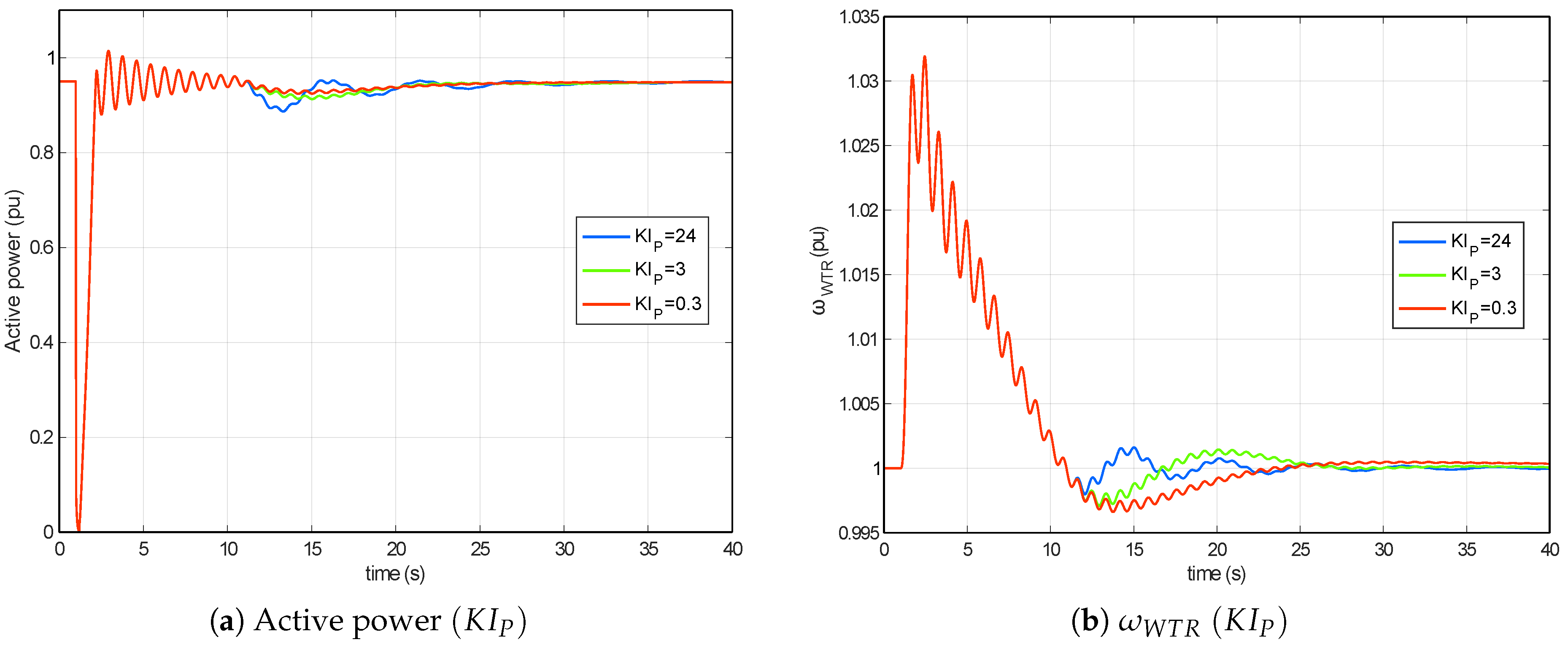
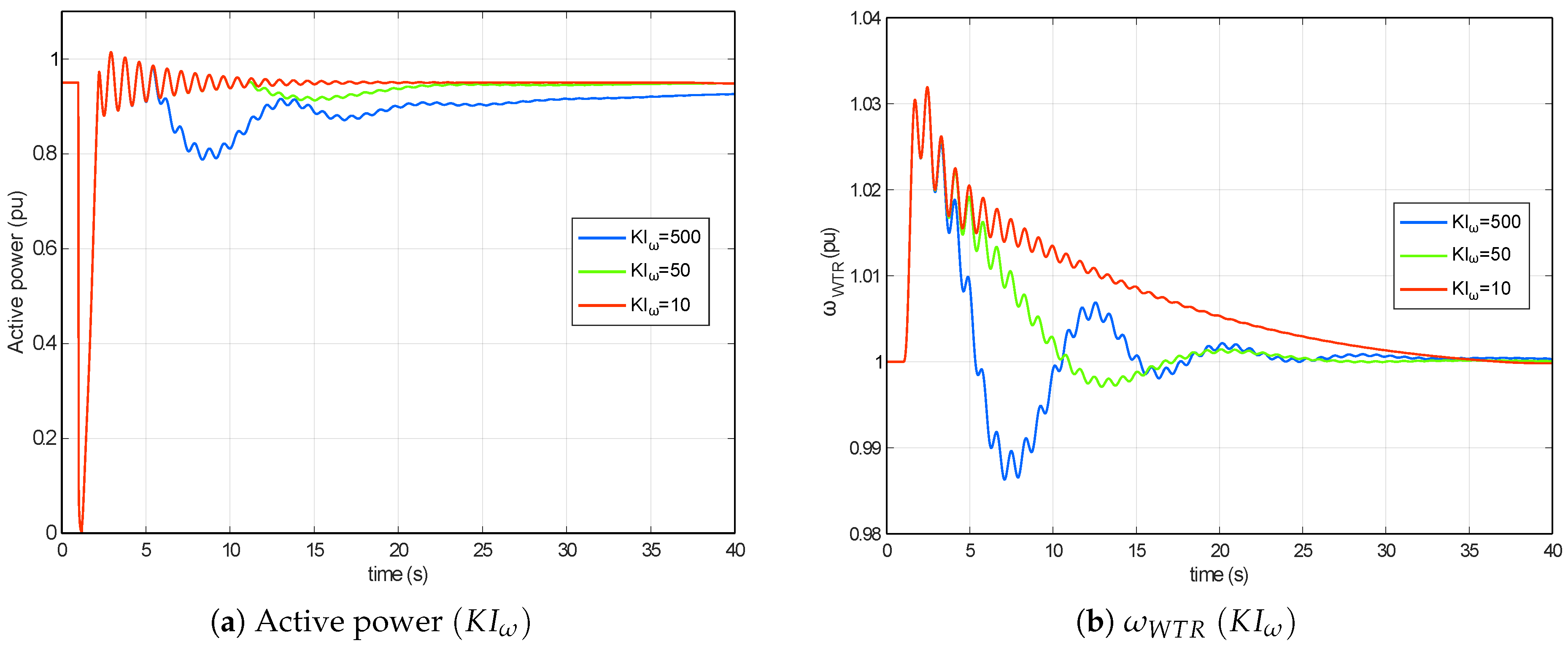
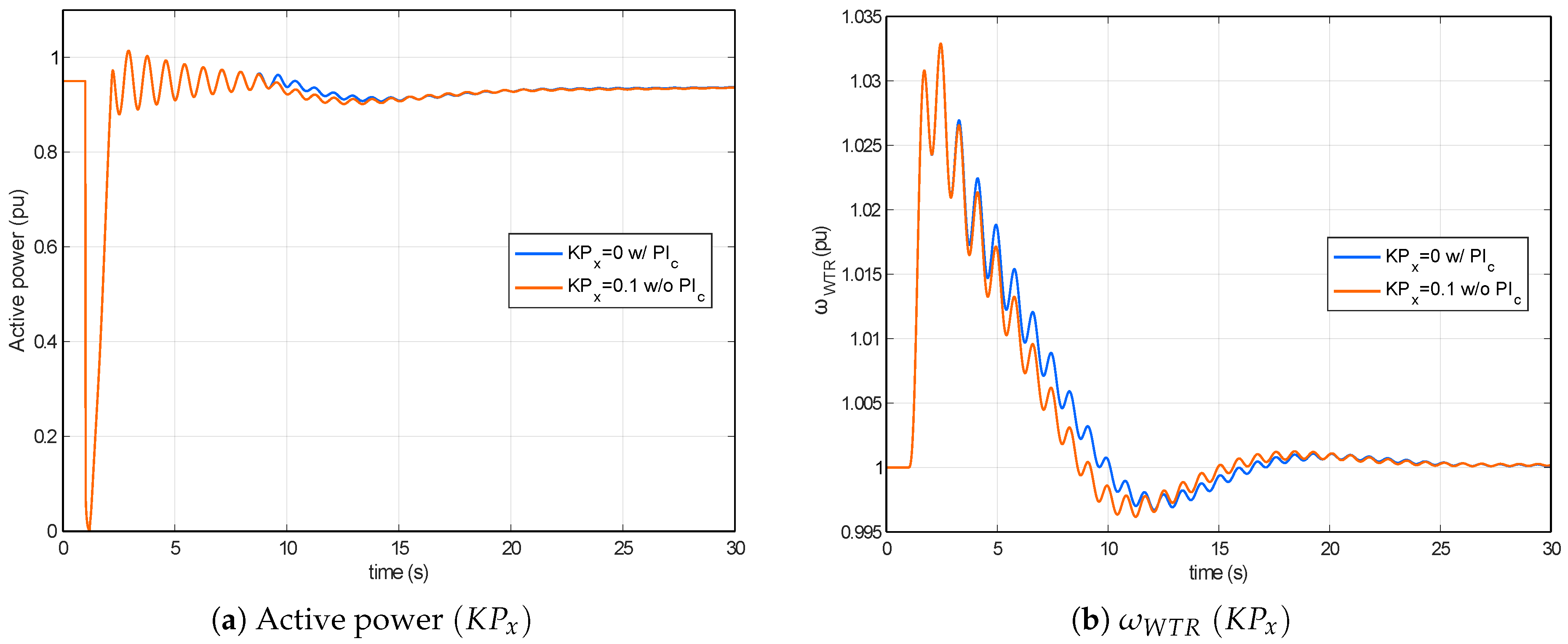
4.1. Active Power Control Model

Active power control is included in the control system of the wind turbine. Figure 12 shows the block diagram of the active power control model implemented in MATLAB/Simulink. The inputs of the system are the following:

• ${\omega }_{WTR}$ and ${\omega }_{gen}$: rotational speed values from the two mass model discussed in Section 3.
• $p_{WT,ref}$: active power reference to be injected into the grid by the WT (manually adjusted).
• $P_{WT}$: active power obtained from the electrical generator system.
• $u_{WT}$: voltage reference from the electrical generator system.
• $i_{p,max}$: maximum active current able to be injected into the grid by the WT as determined by the current limitation system.

The WT active power is filtered by using $Tp\_filt$. This filter avoids sudden changes in the reference speed. Moreover, if this constant is set to an extremely high value, it allows keeping a fixed reference rotational speed during the entire simulation, representing a specific operational model. This filtered active power reference goes through a look-up table, which represents the rotational speed at which the generator must rotate when providing a certain active power value. A common look-up table for this system is shown in Figure 13, as well as a table with conventional values [34]. This table summarizes four operation zones for a Type 3 wind turbine:

• Zone 1, where the minimum rotational speed has been reached (${\omega }_{1-2}$) and consequently cannot decrease further due to component limits, mainly converter maximum slip.
• Zone 2, this operation mode covers the minimum rotational speed (${\omega }_{1-2}$) to the rated rotational speed, where the wind turbine operates at its maximum power tracking.
• Zone 3, operation mode maintaining a fixed rated speed (${\omega }_{3-4}$) and below the rated active power. In some cases, instead of a fixed rated rotational speed, there is a linear rotational speed variation to achieve the rated rotational speed at the rated active power [35].
• Zone 4, this last operation mode is set at the rated rotational speed (${\omega }_{3-4}$) and the rated active power. Dotted lines included in Figure 13a imply that, under simulation conditions, the active power reference presents a certain slope, simplifying the model and offering more stable simulations; although under real control conditions, this look-up table has the two vertical lines originally indicated.

These reference look-up tables are conventionally defined by the wind turbine generator torque [36]. However, the corresponding IEC uses an active power reference. For this reason, the values provided in this work are related to $P_{WT}$.

The rotational speed reference ${\omega }_{ref}$ is filtered by the $T\omega \_ref$, which can present a similar function to the active power filter ($Tp\_filt$). Differences between ${\omega }_{WTR}$ and ${\omega }_{ref}$ are determined, and then, a rotational speed error is estimated. In order to model real wind turbine controller filters, the IEC 61400-27-1 allows using a first order filter $T\omega \_gen$ for ${\omega }_{gen}$. Considering that these models of a real wind turbine only have the drive train resonant frequency as perturbation, this filter is intended to filter these oscillations. However, the simplicity of a first-order filter as the low pass filter does not efficiently meet the drive train perturbations. As a contribution of the authors to the future IEC version to be published in 2018, the new version will include an option to choose between ${\omega }_{WTR}$ and ${\omega }_{gen}$ as an input to the proportional-integral (PI) torque controller. Therefore, ${\omega }_{WTR}$ is chosen as a simplified way to determine a ${\omega }_{gen}$ filtered value. It is usually associated with the application of drive train damping. However, ${\omega }_{gen}$ is used if the drive train damping function is achieved using the torque PI itself, instead of the drive train damping function $K_{DTD}=0$. This ${\omega }_{WTR}$ or ${\omega }_{gen}$ is then considered as the main input to the torque PI subsystem, as shown in the upper right region of Figure 12. The other input to the torque PI subsystem is the maximum electromagnetic torque $\left({\tau }_{e,max}\right)$ to be provided by the WT. It is determined by the relation between $p_{WT,ref}$ and ${\omega }_{WTR}$. As an additional contribution of the authors, the future version of Standard IEC 61400-27-1 [9] to be published in 2018 will also define the use of ${\omega }_{WTR}$ or ${\omega }_{ref}$ going through a filter. However, the oscillations of ${\omega }_{WTR}$ are much smaller, and hence, the performance of the system is more accurate. Taking into account that Standard IEC 61400-27-1 has been developed recently, very few model implementations can be found in the specific literature, and thus, the current work contributes significantly to the IEC improvements.

Figure 14 shows the torque PI subsystem. This control system gives an output proportional to the rotational speed error by adding the minimum between:

• A ramp with a constant slope defined by the parameter $dtau\_max$. This ramp function is only used under voltage dip conditions.
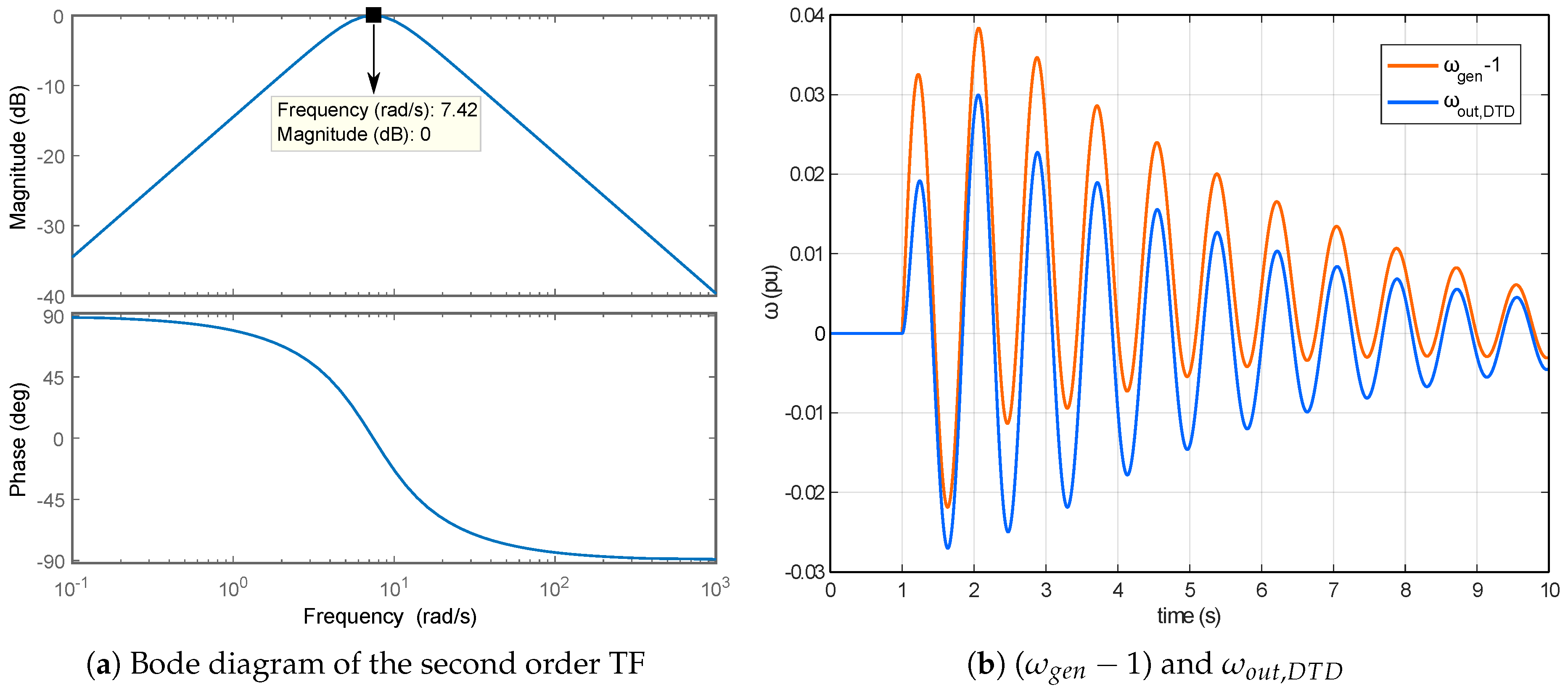
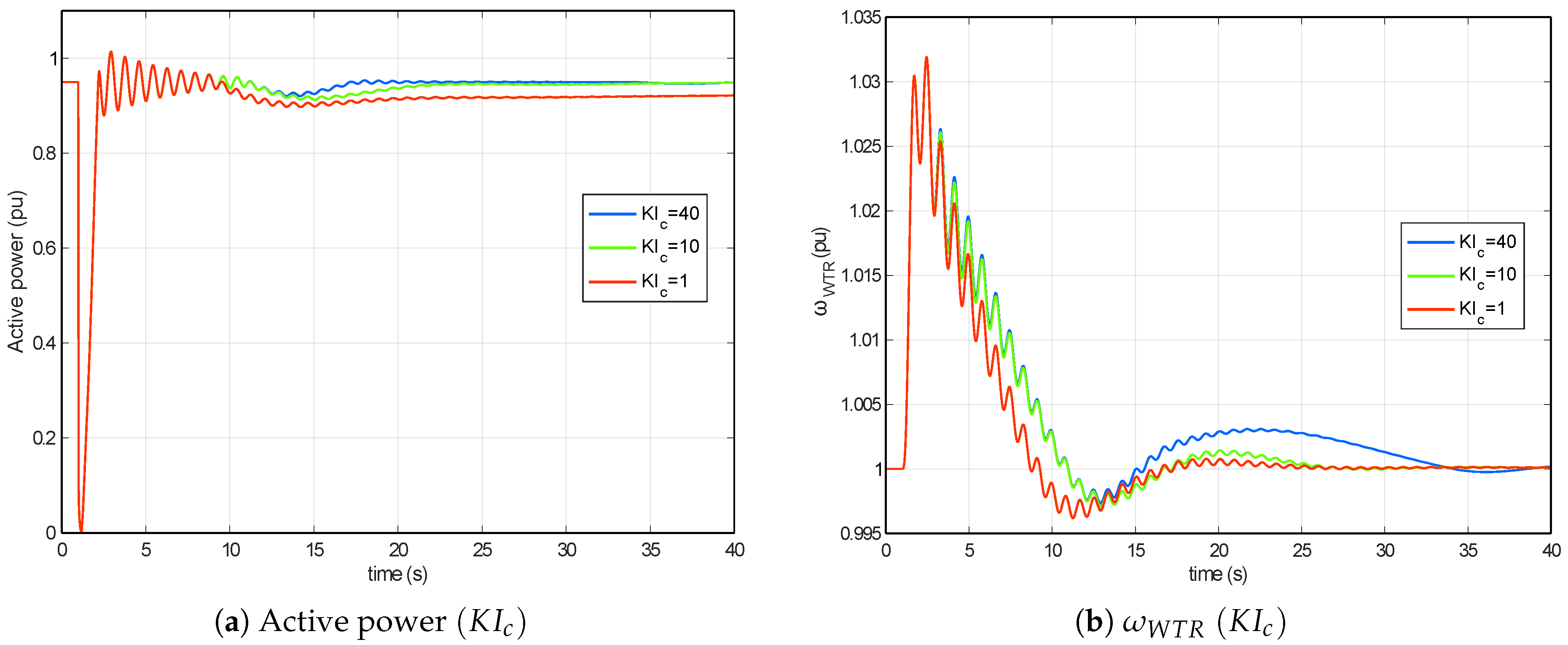
• The torque output filtered by an integral controller with a constant estimated as $K{I}_p/K{P}_p$.

The ${\tau }_{out}$ output is saturated between ${\tau }_{e,max}/{\tau }_{e,min}$, returning to the main control system. This torque is multiplied by the generation rotational speed, obtaining an active power signal. The rate active power and the value of this signal is saturated and filtered, and then, the active power command signal, which is used by the rest of the control systems, is obtained [37]. An additional signal from the Drive Train Damping (DTD) system is added to the estimated output [32]. This control system provides an electrical torque accounting for the natural damping by considering speed differences between both low and high speed shafts. It is modeled through a second-order transfer function as follows,

$$T{F}_{DTD}={\displaystyle \frac{2·\xi ·{\omega }_{DTD}·s}{s^2+2·\xi ·{\omega }_{DTD}·s+{\omega }_{DTD}^2}},$$

(4)

where ${\omega }_{DTD}$ is determined as the frequency of the two mass model oscillations; see Equation (3). This system thus compensates the mechanical oscillations by adding an oscillating electrical power and then producing a highly efficient damping effect.

Figure 15 shows the effects of the $K{P}_P$ parameter of the torque PI controller. The decrease in this proportional parameter involves a more under-damped behavior with higher overshoot. This behavior increases due to the inverse influence of $K{P}_P$ in the integral gain of the controller. The responses of the system when parameter $K{I}_P$ is modified are shown in Figure 16. Increasing $K{I}_P$ produces a more oscillating response. The overshoot in ${\omega }_{WTR}$ is decreased for higher $K{I}_P$ values, although the active power response is oscillating much more.

Figure 17 shows the active power and ${\omega }_{WTR}$ responses when the DTD system is not considered ($K_{DTD}=0$). The influence of the DTD system can be easily observed, damping the oscillations at a high rate. The second-order transfer function used to model this subsystem constitutes a band-pass filter, the tuning frequency of which is the natural frequency of the mechanical system. The addition of an oscillating active power with this frequency dampens the natural oscillations caused by the interaction between high and low speed shafts. Figure 18a shows a Bode Diagram of this transfer function for the original system parameters, which involves a natural frequency ${\omega }_{DTD}=7.4162$ rad/s. As the input to the transfer function is ${\omega }_{gen}$ itself, the harmonic components of this frequency are almost negligible, and thus, the TF damping coefficient is not of great importance in the response of this system. This absence of harmonic components also implies that, in the case of a bad tuning in the frequency of the TF, the filter will not allow the oscillation to pass through, and hence, the effect will be equivalent to reducing $K_{DTD}$ to zero, thus deactivating the system. Figure 18b shows (${\omega }_{gen}-1$); the mean value of 1 pu is subtracted in order to compare between the DTD system output and the output from the band pass filter. Both signals have the same frequency, and the band pass filter also dampens the acceleration due to the voltage dip. Under steady-state operation conditions, the output of this subsystem is considered as zero. The filter output is saturated and directly considered as an active power signal added to the active power obtained from the torque PI subsystem output.

This active power constitutes the main output of the $P_{Ctrl}$ system ($p_{ord}$). The active current input to the electrical generator system is then estimated by dividing $p_{ord}$ by the voltage signal. An alternative method can be considered using ${\omega }_{gen}$ instead of ${\omega }_{WTR}$ as torque PI input, and with $K_{DTD}=0$. However, this option has some drawbacks:

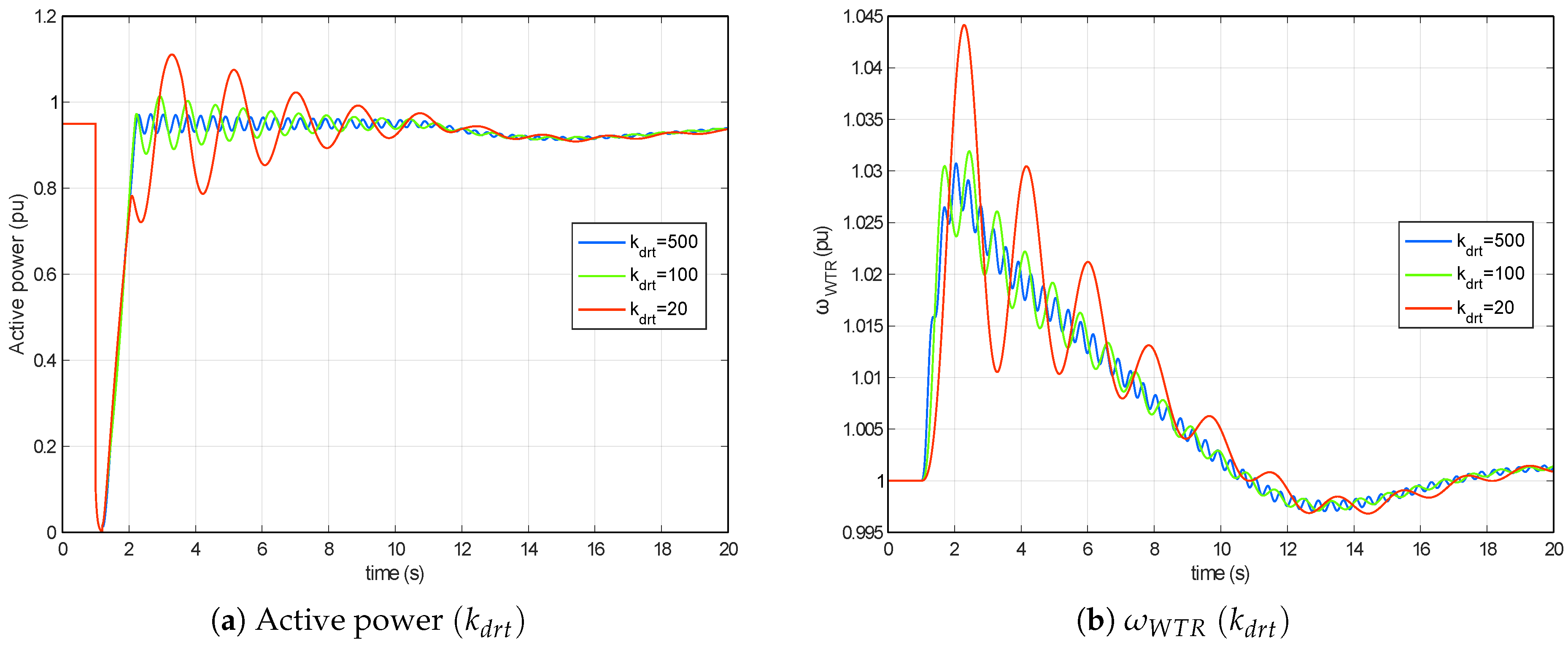
• The oscillation amplitude is larger since $K{I}_P$ is significantly higher than $K_{DTD}$, and thus, the system may become unstable.
• The drive train oscillation is delayed by the $Tp\_ord$ filter, which models the converter time response. The addition of this phase to the system means the drive train damping is less efficient than if the drive train damper function injects after $Tp\_ord$.

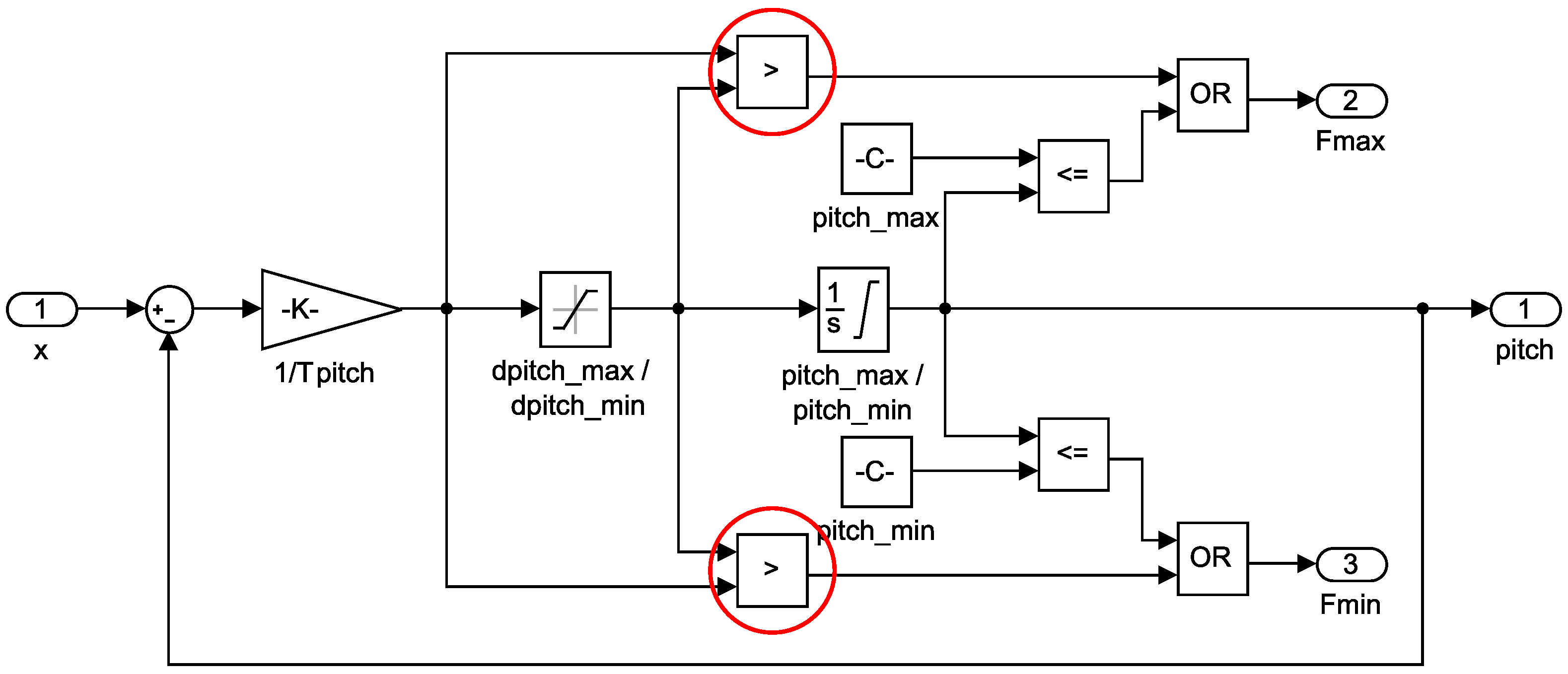
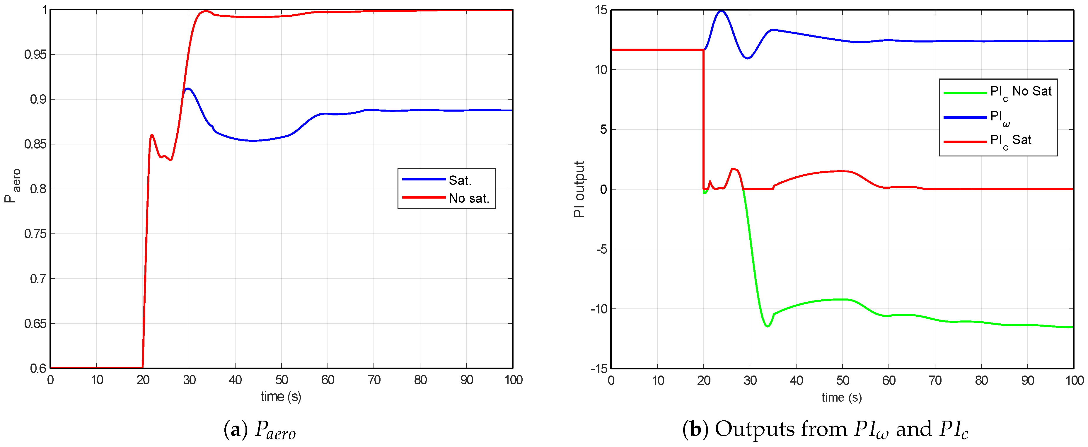
4.2. Pitch Control Model

The pitch control model is mainly formed by the addition of two PI controllers, usually depending on the WT rotor rotational speed and the active power reference provided by the active power control model [38,39], $w_{WTR}$ and $p_{ord}$ respectively in Figure 19. A cross-coupling between both controllers is considered as a proportional gain $K{P}_x$ commonly included by manufacturers to obtain more robust WT control.

Figure 20 shows the first order filter with limitation detection (D.10) system. Highlighted relational operator blocks represent two comparison blocks. According to IEC 61400-27-1 [9], these comparison blocks are ≥. However, if the equal sign is kept in the blocks, the anti wind-up protection system will be active under normal operation, due to the pitch rate limit not actuating, and hence, its inputs and outputs will be equal. When the anti wind-up protection system performs properly, the signals $F_{max}$ and $F_{min}$ are activated either when the pitch rate is too high or too low, respectively, or when the pitch value itself is higher or lower than the maximum and minimum WT pitch. This modification proposed by the authors is currently under study to be included in the second edition of IEC 61400-27-1, which is expected to be issued in February 2018.

The $F_{max}$ and $F_{min}$ signals are inputs to the anti wind-up integrator system, as can be seen in Figure 21. They disable the integral actuation by the action of saturator blocks, limiting the error signal to zero. Standard IEC 61400-27-1 [9] indicates that the integrator included in this system may be saturated in order to control the output of each controller. However, for the current work, these outputs will not be saturated (limits are set to infinite) in order to allow the maximum interaction between both controllers.

Table 1 summarizes the analyzed parameters under voltage dips. For the pitch control system, when the proportional gains of the controllers are increased keeping the rest of the gains constant, the model’s response is faster than the response with lower proportional gain (unless these gains are too large and the system becomes unstable). Consequently, these performances have not been included in the paper. However, changes in the controller integral gains have a considerable effect shown in the following figures. Figure 22 depicts the responses when the parameter $K{I}_{\omega }$ is changed. When considering the different $K{I}_{\omega }$ values, the ${\omega }_{WTR}$ evolution along the disturbance is predictable, because the higher the integral gain is, the more under-damped it is, thus being faster and with a higher over-shoot. However, the active power response is detrimental to ${\omega }_{WTR}$, being much slower and unstable when $K{I}_{\omega }$ rises.

By contrast, an adverse reaction to the response of ${\omega }_{WTR}$ occurs when the active power controller integral gain $K{I}_c$ is modified, as shown in Figure 23. The active power response is then faster when $K{I}_c$ is increased, detrimentally affecting the response of ${\omega }_{WTR}$. It is worth noting this interaction as the systems depend on different error signals. Moreover, under the $K{P}_x=0$ condition corresponding to the simulations in this paper, these systems are completely independent. Therefore, neither controller can be adjusted separately, due to the behavior of one having a considerable impact on the other as a consequence of the multiple dependences with the rest of control systems.

Finally, we have also studied the influence of the use of both PI controllers as compared to the use of the cross-coupling parameter $K{P}_x$. Theoretically, and according to the block models shown in Figure 19, if the following condition is fulfilled,

$${\displaystyle \frac{K{I}_c}{s}}+K{P}_c=K{P}_x·\left({\displaystyle \frac{K{I}_{\omega }}{s}}+K{P}_{\omega }\right),$$

(5)

the behavior of both topologies should be equal. However, as shown in Figure 24, the two responses are not the same. This is due to the presence of the ramp limiters (and possibly value saturators) in the anti wind-up integrator systems; see Figure 21. If each error signal goes through its own controller, the possibility of reaching the saturation value is lower than if both signals are added and then the value goes through just one controller. This case is depicted in the example in Figure 24, in which the addition of both errors results in a high value, which is saturated if the cross-coupling method is used. However, if both controllers are used, the signals of each one fail to reach the ramp limiters, or even the value saturators if they are used. These considerations involve slight differences between the systems.

As previously mentioned, the cross-coupling gain is commonly used by manufacturers to obtain stable control of the wind turbine. The addition of two PI controllers may cause coordination issues in some situations, which have been detected by the authors. For example, if the wind turbine is working in Zone 4, as in Figure 13, an active power increase is set by the control (still remaining in Zone 4), the $P{I}_{\omega }$ controller will not actuate since the ${\omega }_{ref}$ reference would be the same in both situations, but $P{I}_C$ will decrease its output. However, if this output was originally close to zero, it can become a negative value, and if the saturations of the standard are considered, the pitch angle would never reach its reference. Figure 25 shows this performance. In $t=20$ s, the active power reference changes from 0.6 pu to 1 pu; the $P{I}_{\omega }$ output keeps constant under steady-state conditions, but the $P{I}_c$ output decreases the pitch angle to achieve the new active power reference (1 pu). As shown in Figure 25a, if the controller is saturated, the final $P_{aero}$ of 1 pu is not achieved, and then, the wind turbine response is incorrect. This problem is solved by the use of $K{P}_x$, because only $P{I}_{\omega }$ is working, and subsequently, these coordination problems disappear.

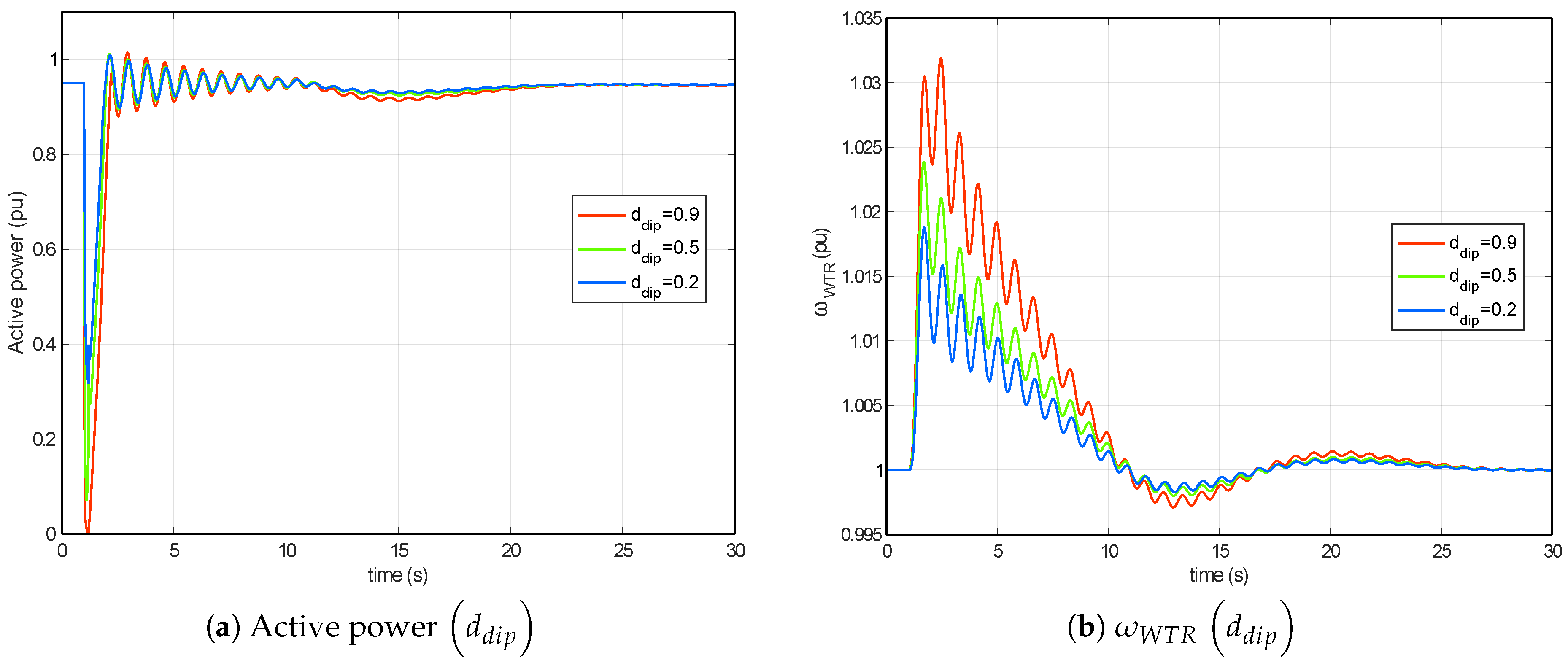
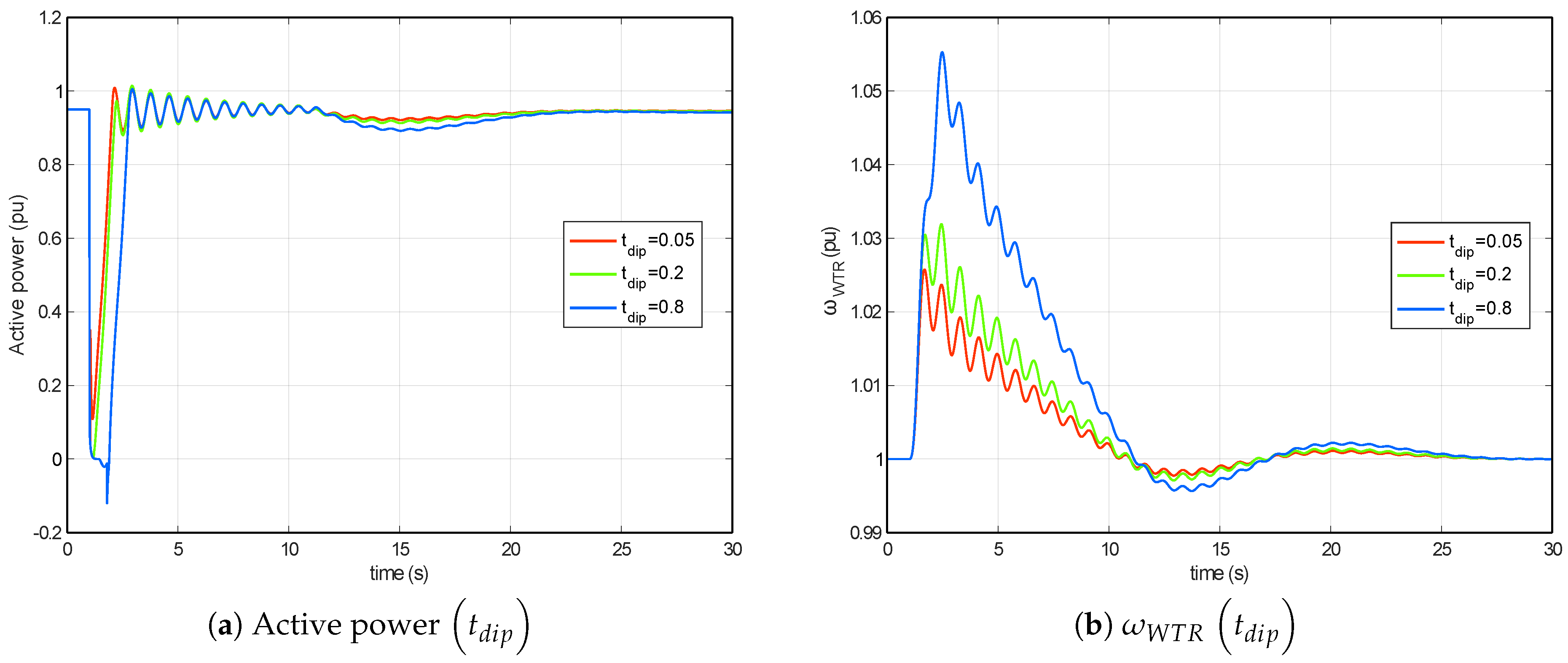
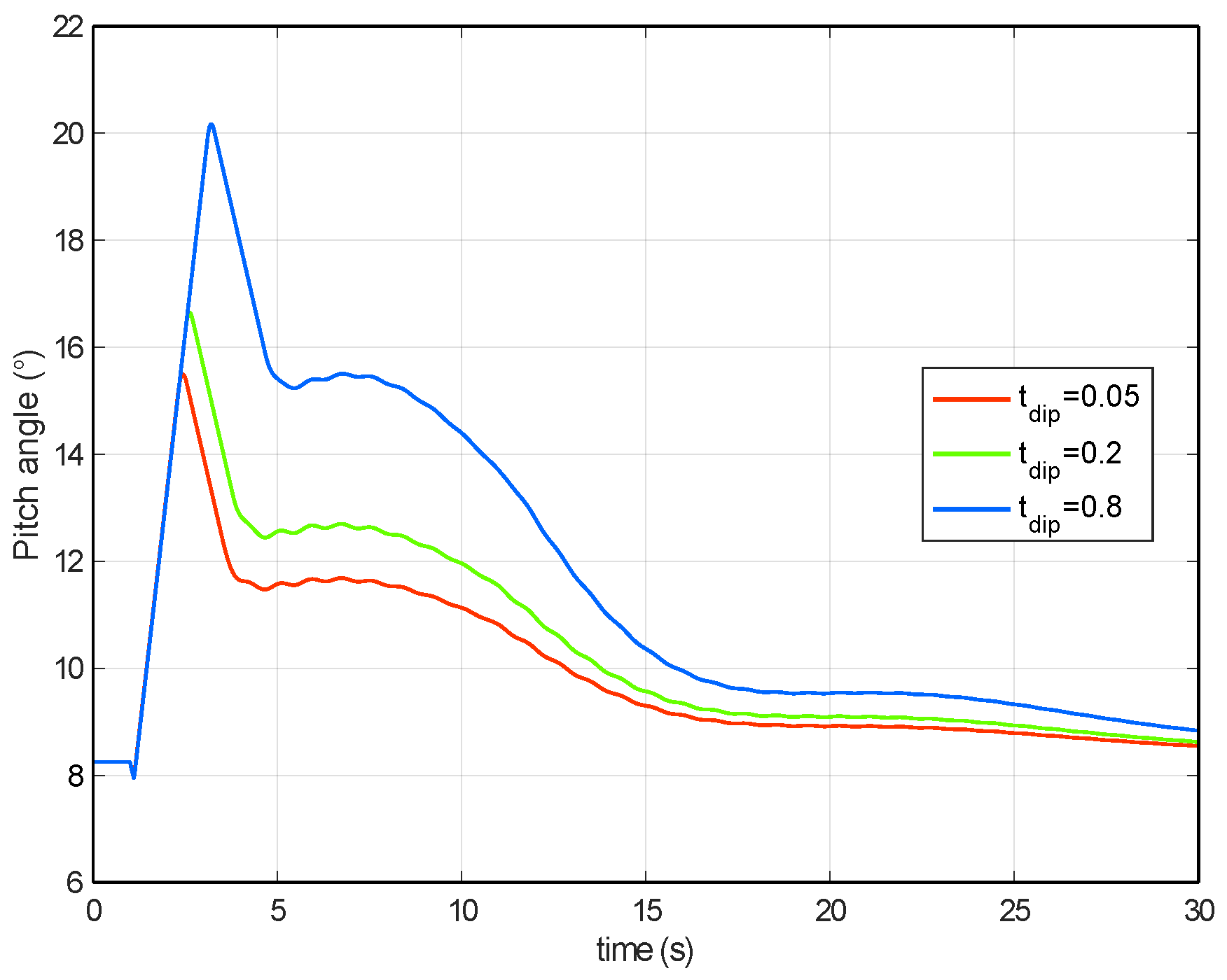
5. Influence of Voltage Dip Characteristics: Depth and Duration

According to [40], a voltage dip is a temporary reduction of the root-mean-square (rms) voltage at a point in the electrical system below a given threshold. It is mainly characterized by two parameters: (i) depth, defined as the difference between the rms-voltage reference and the minimum rms-voltage achieved during the event and generally expressed as a percentage of the rms-voltage reference; (ii) and duration, which is the time between the rms-voltage dropping below the threshold given by the corresponding grid-code and the rms-voltage being recovered above the threshold. In this section, the effects of the variation in depth and duration of the voltage dip on the WT response are discussed in detail. The ranges of variation for depth and duration are summarized in

Table 2. Voltage dip parameter variations.

Parameter	Original Value	Variation Range
Depth $\left(d_{dip}\right)$	$90\%$	$\left[0.90.50.2\right]$
Duration $\left(t_{dip}\right)$	0.2 s	$\left[0.050.20.8\right]$

.

The depth variations of the voltage dip have a slight influence on the response of the model, as shown in Figure 26. For a certain depth, the variation in the response of the active power may seem predictable; however, and according to Figure 26a, there is no linear relation between the depth of the voltage dip and the minimum value of the active power provided by the WT (for example, with a $d_{dip}=0.2$, the minimum active power value is lower than $0.4$ pu), due to the dynamics of the different control systems, as well as to the operation of the crowbar system. An increase in the depth also involves a higher acceleration; see Figure 26b. However, this parameter does not have as much influence as the duration of the dip.

Figure 27 shows the different responses when $t_{dip}$ is increased. The longer the voltage dip, the higher is the value reached by ${\omega }_{WTR}$, because of the lack of electromagnetic torque that counteracts the mechanical torque produced by the wind. This maintained acceleration involves the actuation of $P{I}_{\omega }$ from the pitch control system, increasing the pitch angle in order to limit this acceleration; see Figure 28. This response involves a higher overshoot in rotational speed, which creates an active power reduction when ${\omega }_{WTR}<0$. Then, if we wish to control this response, the values to be changed correspond to the $P{I}_{\omega }$ controller from pitch control, varying the performance during the transient, as was previously discussed in the simulations.

6. Conclusions

A Type 3 WT model previously tested by the authors is adjusted and analyzed to give a complete benchmark response under voltage dips. Values and possible modifications of the parameters are also included in the paper, offering a notable reference for future studies. Parameters corresponding to the mechanical two mass model, the active power control and the pitch angle control models have been widely described, and their influence on the model’s response is analyzed in terms of active power and rotational speed evolution during the disturbance. Extensive simulations have been carried out by the authors and included in the paper, and the different responses have also been compared. Furthermore, the model’s responses have been discussed in detail, aiming to provide a better understanding of these recent complex generic models based on IEC 61400-27-1.

The two mass model parameters affect the physical response of the system, varying the frequency and amplitude of the oscillations of both active power and rotational speed under disturbances. For the active power control system, the response of the model can be adjusted by the PI parameter selection. Key results are obtained from the drive train damping system, which allows a significant damping effect by the injection of an oscillating active power with the same frequency as the mechanical oscillations. Regarding the pitch control model, the influence of the increase in the integral gain of the controllers also yields significant results, since the improvement in the behavior of one influences the proper response of the signal controlled by the other. The effect of a cross-coupling gain is also included in this analysis. In this way, and although theoretically there should be no difference, the behavior varies slightly between the two simulations due to the limiters included in the model.

This paper thus provides practical and complete parameters and simulations for a Type 3 WT model based on IEC 61400-27-1 submitted to voltage dips. Results and parameters are of significant interest to researchers and wind turbine manufacturers currently working on the definition and adjustment of this type of model.

References

1. Amin, A. REmap: Roadmap for a Renewable Energy Future; Technical Report; International Renewable Energy Agency (IRENA): Abu Dhabi, UAE, 2016. [Google Scholar]
2. Mueller, S. Next Generation Wind and Solar Power; Technical Report; International Energy Agency (IEA): Paris, France, 2016.
3. Philibert, C.; Holttinen, H. Technology Roadmap Wind Energy; Technical Report; International Energy Agency (IEA): Paris, France, 2013.
4. Honrubia-Escribano, A.; Jiménez-Buendía, F.; Molina-García, A.; Fuentes-Moreno, J.; Muljadi, E.; Gómez-Lázaro, E. Analysis of Wind Turbine Simulation Models: Assessment of Simplified versus Complete Methodologies. In Proceedings of the XVII International Symposium on Electromagnetic Fields in Mechatronics, Electrical and Electronic Engineering, Valencia, Spain, 10–12 September 2015; p. 8. [Google Scholar]
5. Honrubia Escribano, A.; Gomez-Lazaro, E.; Fortmann, J.; Sørensen, P.; Martín-Martínez, S. Generic dynamic wind turbine models for power system stability analysis: A comprehensive review. Renew. Sustain. Energy Rev. 2017, in press. [Google Scholar] [CrossRef]
6. Liu, Y.J.; Chen, P.A.; Lan, P.H.; Chang, Y.T. Dynamic simulation and analysis of connecting a 5 MW wind turbine to the distribution system feeder that serves to a wind turbine testing site. In Proceedings of the 2017 IEEE 3rd International Future Energy Electronics Conference and ECCE Asia (IFEEC 2017-ECCE Asia), Kaohsiung, Taiwan, 3–7 June 2017; pp. 2031–2035. [Google Scholar]
7. Asmine, M.; Brochu, J.; Fortmann, J.; Gagnon, R.; Kazachkov, Y.; Langlois, C.E.; Larose, C.; Muljadi, E.; MacDowell, J.; Pourbeik, P.; et al. Model Validation for Wind Turbine Generator Models. IEEE Trans. Power Syst. 2011, 26, 1769–1782. [Google Scholar] [CrossRef]
8. Fortmann, J.; Engelhardt, S.; Kretschmann, J.; Feltes, C.; Erlich, I. New Generic Model of DFG-Based Wind Turbines for RMS-Type Simulation. IEEE Trans. Energy Convers. 2014, 29, 110–118. [Google Scholar] [CrossRef]
9. International Electrotechnical Commission. IEC 61400-27-1: Electrical Simulation Models for Wind Power Generation—Wind Turbines; International Electrotechnical Commission: Geneva, Switzerland, 2015. [Google Scholar]
10. Villena-Ruiz, R.; Lorenzo-Bonache, A.; Honrubia-Escribano, A.; Gómez-Lázaro, E. Implementation of a generic Type 1 wind turbine generator for power system stability studies. In Proceedings of the International Conference on Renewable Energies and Power Quality, Malaga, Spain, 4–6 April 2017. [Google Scholar]
11. Das, K.; Hansen, A.; Sørensen, P. Understanding IEC standard wind turbine models using SimPowerSystems. Wind Eng. 2016, 40, 212–227. [Google Scholar] [CrossRef] [Green Version]
12. Sørensen, P. IEC 61400-27. Electrical Simulation Models for Wind Power Generation; European Energy Research Alliance (EERA): Brussels, Belgium, 2012. [Google Scholar]
13. Honrubia-Escribano, A.; Gómez-Lázaro, E.; Jiménez-Buendía, F.; Muljadi, E. Comparison of Standard Wind Turbine Models with Vendor Models for Power System Stability Analysis. In Proceedings of the 15th International Workshop on Large-Scale Integration of Wind Power into Power Systems as well as on Transmission Networks for Offshore Wind Power Plants, Vienna, Austria, 15–17 November 2016. [Google Scholar]
14. Göksu, O.; Altin, M.; Fortmann, J.; Sorensen, P. Field Validation of IEC 61400-27-1 Wind Generation Type 3 Model with Plant Power Factor Controller. IEEE Trans. Energy Convers. 2016, 31, 1170–1178. [Google Scholar] [CrossRef]
15. Honrubia Escribano, A.; Gómez-Lázaro, E.; Vigueras-Rodríguez, A.; Molina-García, A.; Fuentes, J.A.; Muljadi, E. Assessment of DFIG simplified model parameters using field test data. In Proceedings of the IEEE Symposium on Power Electronics & Machines for Wind Application, Denver, CO, USA, 16–18 July 2012; pp. 1–7. [Google Scholar]
16. Sørensen, P.; Andersen, B.; Bech, J.; Fortmann, J.; Pourbeik, P. Progress in IEC 61400-27. Electrical Simulation Models for Wind Power Generation. In Proceedings of the 11th International Workshop on Large-Scale Integration of Wind Power into Power Systems as well as on Transmission Networks for Offshore Wind Power Plants, Lisbon, Portugal, 13–15 November 2012; p. 7. [Google Scholar]
17. Bech, J. Siemens Experience with Validation of Different Types of Wind Turbine Models. In Proceedings of the IEEE Power and Energy Society General Meeting, Washington, DC, USA, 27–31 July 2014. [Google Scholar]
18. Jiménez Buendía, F.; Barrasa Gordo, B. Generic Simplified Simulation Model for DFIG with Active Crowbar. In Proceedings of the 11th International Workshop on Large-Scale Integration of Wind Power into Power Systems as well as on Transmission Networks for Offshore Wind Power Plants, Lisbon, Portugal, 13–15 November 2012; p. 6. [Google Scholar]
19. Honrubia-Escribano, A.; Jiménez-Buendía, F.; Gómez-Lázaro, E.; Fortmann, J. Field Validation of a Standard Type 3 Wind Turbine Model for Power System Stability, According to the Requirements Imposed by IEC 61400-27-1. IEEE Trans. Energy Convers. 2017. [Google Scholar] [CrossRef]
20. Zeni, L.; Gevorgian, V.; Wallen, R.; Bech, J.; Sørensen, P.E.; Hesselbæk, B. Utilisation of real-scale renewable energy test facility for validation of generic wind turbine and wind power plant controller models. IET Renew. Power Gener. 2016, 10, 1123–1131. [Google Scholar] [CrossRef]
21. Lorenzo-Bonache, A.; Villena-Ruiz, R.; Honrubia-Escribano, A.; Gómez-Lázaro, E. Real time simulation applied to the implementation of generic wind turbine models. In Proceedings of the International Conference on Renewable Energies and Power Quality, Malaga, Spain, 4–6 April 2017. [Google Scholar]
22. Honrubia-Escribano, A.; Jiménez-Buendía, F.; Gómez-Lázaro, E.; Fortmann, J. Validation of Generic Models for Variable Speed Operation Wind Turbines Following the Recent Guidelines Issued by IEC 61400-27. Energies 2016, 9, 1048. [Google Scholar] [CrossRef]
23. Göksu, O.; Sørensen, P.; Morales, A.; Weigel, S.; Fortmann, J.; Pourbeik, P. Compatibility of IEC 61400-27-1 Ed 1 and WECC 2nd Generation Wind Turbine Models. In Proceedings of the 15th Wind Integration Workshop, Vienna, Austria, 15–17 November 2016. [Google Scholar]
24. Hernández, C.V.; Telsnig, T.; Pradas, A.V. JRC Wind Energy Status Report 2016 Edition; Market, Technology and Regulatory Aspects of Wind Energy; JRC Science for Policy Report; European Commission: Brussels, Belgium, 2017. [Google Scholar]
25. Fortmann, J.; Engelhardt, S.; Kretschmann, J.; Janben, M.; Neumann, T.; Erlich, I. Generic Simulation Model for DFIG and Full Size Converter based Wind Turbines. In Proceedings of the 9th International Workshop on Large-Scale Integration of Wind Power into Power Systems as well as on Transmission Networks for Offshore Wind Plants, Quebec, QC, Canada, 18–19 October 2010; p. 8. [Google Scholar]
26. Lorenzo-Bonache, A.; Villena-Ruiz, R.; Honrubia-Escribano, A.; Gómez-Lázaro, E. Comparison of a Standard Type 3B WT Model with a Commercial Build-in Model. In Proceedings of the IEEE International Electric Machines & Drives Conference, Miami, FL, USA, 21–24 May 2017. [Google Scholar]
27. Subramanian, C.; Casadei, D.; Tani, A.; Sorensen, P.; Blaabjerg, F.; McKeever, P. Implementation of Electrical Simulation Model for IEC Standard Type-3A Generator. In Proceedings of the 2013 European Modelling Symposium (EMS), Manchester, UK, 20–22 November 2013; pp. 426–431. [Google Scholar]
28. European Commission. EU 2016/631 of 14 April 2016 Establishing a Network Code on Requirements for Grid Connection of Generators; European Commission: Brussels, Belgium, 2016. [Google Scholar]
29. Morales, A.; Robe, X.; Maun, J.C. Wind Turbine Generator Systems. Part 21. Measurement and Assessment of Power Quality Characteristics of Grid Connected Wind Turbines; IEC/CEI: Geneva, Switzerland, 2001. [Google Scholar]
30. Muyeen, S.; Ali, M.; Takahashi, R.; Murata, T.; Tamura, J.; Tomaki, Y.; Sakahara, A.; Sasano, E. Comparative study on transient stability analysis of wind turbine generator system using different drive train models. IET Renew. Power Gener. 2007, 1, 131–141. [Google Scholar] [CrossRef]
31. Perdana, A. Dynamic Models of Wind Turbines. A Contribution towards the Establishment of Standardized Models of Wind Turbines for Power System Stability Studies. Ph.D. Thesis, Chalmers University of Technology, Gothenburg, Sweden, 2008. [Google Scholar]
32. Fortmann, J. Modeling of Wind Turbines with Doubly Fed Generator System. Ph.D. Thesis, Department for Electrical Power Systems, University of Duisburg-Essen, Duisburg, Germany, 2014. [Google Scholar]
33. Behnke, M.; Ellis, A.; Kazachkov, Y.; McCoy, T.; Muljadi, E.; Price, W.; Sanchez-Gasca, J. Development and validation of WECC variable speed wind turbine dynamic models for grid integration studies. In Proceedings of the AWEA Wind Power Conference, Los Angeles, CA, USA, 4–7 June 2007; pp. 1–5. [Google Scholar]
34. Burton, T.; Sharpe, D.; Jenkins, N.; Bossanyi, E. Wind Energy Handbook; John Wiley & Sons: Hoboken, NJ, USA, 2001; p. 642. [Google Scholar]
35. Bossanyi, E.A. The Design of Closed Loop Controllers for Wind Turbines. Wind Energy 2000, 3, 149–163. [Google Scholar] [CrossRef]
36. Wright, A.D.; Fingersh, L.J. Advanced Control Design for Wind Turbines. Part I: Control Design, Implementation, and Initial Tests; Technical Report; NREL: Golden, CO, USA, 2008.
37. Lorenzo-Bonache, A.; Villena-Ruiz, R.; Honrubia-Escribano, A.; Gómez-Lázaro, E. Operation of Active and Reactive Control Systems of a Generic Type 3 WT Model. In Proceedings of the IEEE International Conference on Compatibility, Power Electronics and Power Engineering, Cadiz, Spain, 4–6 April 2017. [Google Scholar]
38. Lin, L.; Zhang, J.; Yang, Y. Comparison of Pitch Angle Control Models of Wind Farm for Power System Analysis. In Proceedings of the IEEE Power Energy Society General Meeting, Calgary, AB, Canada, 26–30 July 2009; pp. 1–7. [Google Scholar]
39. Muljadi, E.; Butterfield, C.P. Pitch-controlled variable-speed wind turbine generation. IEEE Trans. Ind. Appl. 2001, 37, 240–246. [Google Scholar] [CrossRef]
40. Institute of Electrical and Electronics Engineers (IEEE). 1564-2014—IEEE Guide for Voltage Sag Indices; IEEE: New York, NY, USA, 2014; pp. 1–59. [Google Scholar]
Figure 1. Generic Type 3 WT model: MATLAB/Simulink implementation.
Energies 10 01441 g001
Figure 2. Generic Type 3 WT model: electrical generator system.
Energies 10 01441 g002
Figure 3. Generic Type 3 WT model: control system.
Energies 10 01441 g003
Figure 4. One-dimensional aerodynamic model.
Energies 10 01441 g004
Figure 5. Benchmark response of Type 3 WT: reference parameters.
Energies 10 01441 g005
Figure 6. Physical representation of the two mass model.
Energies 10 01441 g006
Figure 7. Two mass model implemented in MATLAB/Simulink.
Energies 10 01441 g007
Figure 8. H W T R parameter analysis: P W T and ω W T R evolution under a voltage dip.
Energies 10 01441 g008
Figure 9. H g e n parameter analysis: P W T and ω W T R evolution under a voltage dip.
Energies 10 01441 g009
Figure 10. k d r t parameter analysis: P W T and ω W T R evolution under a voltage dip.
Energies 10 01441 g010
Figure 11. c d r t parameter analysis: P W T and ω W T R evolution under a voltage dip.
Energies 10 01441 g011
Figure 12. Active power control system implemented in MATLAB/Simulink.
Energies 10 01441 g012
Figure 13. Look-up table ω r e f vs. P W T and conventional values.
Energies 10 01441 g013
Figure 14. Torque PI system implemented in MATLAB/Simulink.
Energies 10 01441 g014
Figure 15. K P P parameter analysis: P W T and ω W T R evolution under a voltage dip.
Energies 10 01441 g015
Figure 16. K I P parameter analysis: P W T and ω W T R evolution under a voltage dip.
Energies 10 01441 g016
Figure 17. K D T D parameter analysis: P W T and ω W T R evolution under a voltage dip.
Energies 10 01441 g017
Figure 18. Bode diagram. DTD system response.
Energies 10 01441 g018
Figure 19. Pitch control model implemented in MATLAB/Simulink.
Energies 10 01441 g019
Figure 20. First order filter with limitation detection (D.10) implemented in MATLAB/Simulink.
Energies 10 01441 g020
Figure 21. Anti wind-up integrator implemented in MATLAB/Simulink.
Energies 10 01441 g021
Figure 22. K I ω parameter analysis: P W T and ω W T R evolution under a voltage dip.
Energies 10 01441 g022
Figure 23. K I c parameter analysis: P W T and ω W T R evolution under a voltage dip.
Energies 10 01441 g023
Figure 24. K P x parameter analysis: P W T and ω W T R evolution under a voltage dip.
Energies 10 01441 g024
Figure 25. Problems with saturators in IEC 61400-27-1 pitch control.
Energies 10 01441 g025
Figure 26. P W T and ω W T R responses under different voltage dip depths.
Energies 10 01441 g026
Figure 27. P W T and ω W T R responses under different voltage dip durations.
Energies 10 01441 g027
Figure 28. Pitch angle under different voltage dip durations.
Energies 10 01441 g028