1. Introduction
The increase in thermal efficiency along with the reduction in pollutant emissions are the most significant challenges faced by the combustion engine industry, as a result of increasingly demanding legislation in most industrialized countries [
1]. This demand is influencing the continuous development of improvement methods within the combustion engine sector. Although different difficulties still need to be addressed, the Stirling engine is one of the most promising engines among those considered by the combustion engine sector as an alternative to conventional internal combustion units. From a thermodynamic point of view, Stirling units are closed-cycle regenerative thermal engines with a gaseous working fluid and external heat supply, whose operation is based on the cyclic compression and expansion of the gas at two different temperature levels. The main features of the Stirling engine include high efficiency, mechanical simplicity, low vibration, low noise levels, and the possibility of using a wide range of heat sources. Stirling engines are also characterized by a low output power-to-weight ratio, slow load ramps, and issues with sealing when using low molecular weight substances [
2].
Many practical applications and theoretical studies have been proposed and completed since the beginning of the 19th century, when Robert Stirling designed a thermal engine aimed at competing with the steam engine. Unfortunately, such applications have rarely proceeded beyond the academic or experimental level. However, newly proposed use of Stirling engines combined with the harnessing of heat from renewable sources is a promising line of research due to the combination of both versatility and efficiency [
3,
4].
Although different studies have contributed to the performance of Stirling engines, some of the most relevant works were published by Senft [
5,
6,
7,
8,
9], who intensively analyzed the performance of Stirling engines using different mechanical models. After comparing different typologies of reciprocating engines, Senft determined that maximum thermal efficiency was achieved by Stirling engines.
Other noteworthy analyzes of the performance of Stirling engines include those based on finite-time thermodynamics [
10,
11,
12,
13,
14,
15,
16,
17,
18,
19,
20,
21,
22]. This theory was initially proposed by Andresen [
23], based on a macroscopic approach developed by considering different characteristic parameters, such as heat conductance, friction coefficients, overall reaction rates, etc., rather than based on a microscopic knowledge of the processes involved.
Regarding heat transfer, a key issue addressed in this paper, the significant influence of the heat transfer laws used in the models over the optimal performance of Stirling engines have been proven [
24,
25], mainly due to the irreversibility of heat transfer. For heat transfer in Stirling engines, Kaushik et al. [
21] and Senft [
7,
8] contributed considerably. The latter proposed an irreversible model based on the finite-time thermodynamics approach to study the performance of Stirling engines, including a model that considered mechanical losses, heat capacities, and heat losses, which were modelled in accordance with a Newtonian heat transfer law.
In this study, given a specific Stirling engine unit with known geometrical parameters and working fluid properties, thermodynamic simulations are developed using numeric models created in MATLAB
® [
26]. The models are used to analyze the engine performance and to compare it with the expected behavior. These simulations allow the study of the operating conditions in the different components in the unit operation.
This paper provides an analysis of a 2.9 kW commercial Stirling engine, model GENOA 03 (GenoaStirling s.r.l.) [
27], which is used for electric power generation and uses pressurized air as a working fluid. A unit of this engine was transferred by the University of Genoa to the University of Seville for experimental analysis. The two following sections are structured to describe the main features, the governing equations, the simulation algorithm, and the relevant results related to the three ideal thermodynamic models used here: the ideal isothermal model, the ideal adiabatic model, and a simple more realistic model. Afterward, a set of modifications to the ideal adiabatic model are proposed, modifying the heat transfer assumptions and incorporating frictional losses to the mass flows. The purpose of these modifications was to simulate the engine behavior with higher accuracy, allowing for the analysis of the performance of different components, such as the regenerator or the cooler, both key components of the Stirling engine in terms of efficiency. Finally, the authors compare the main results obtained using the different approaches.
2. Engine Technical Data
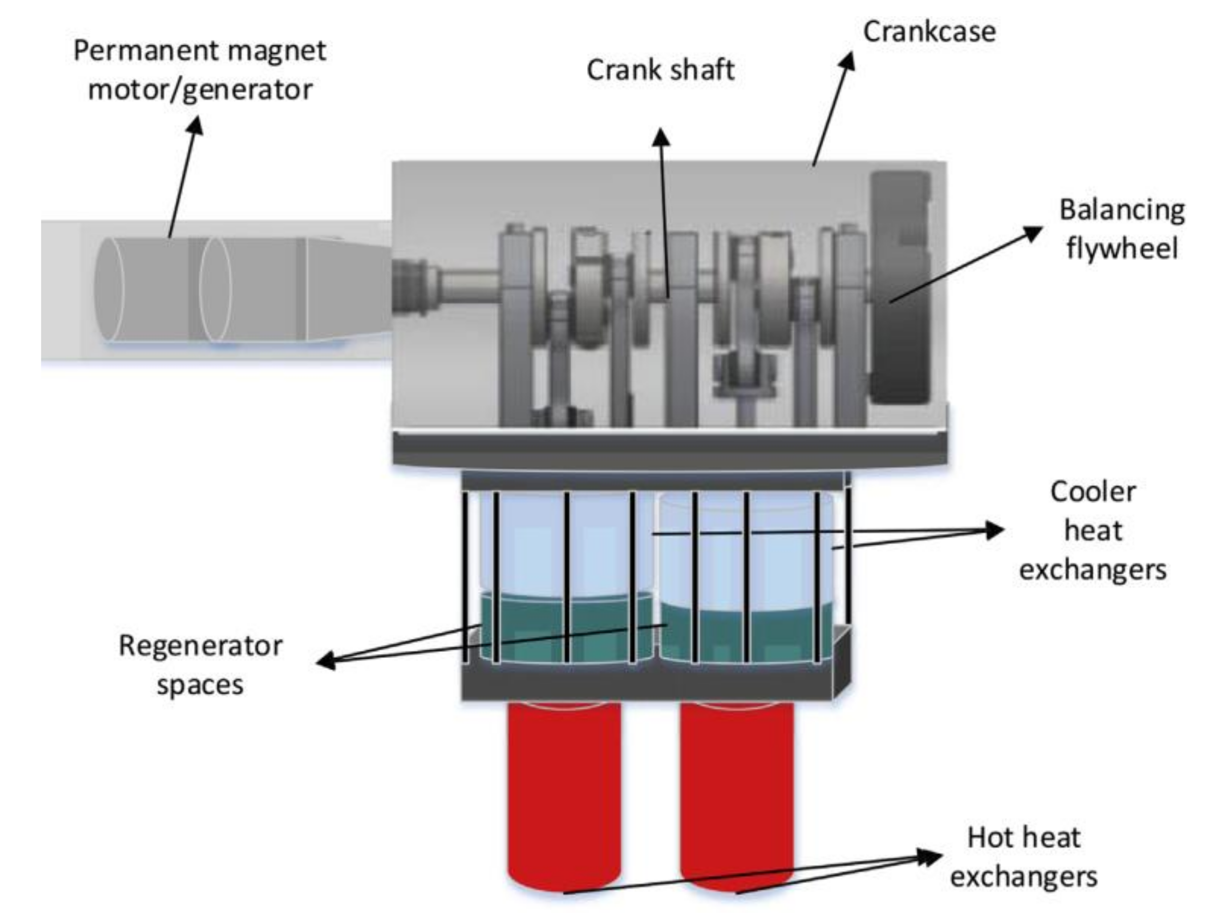
The engine studied is a unit of the model GENOA03, a two-cylinder type alpha Stirling engine, manufactured by the Italian company GenoaStirling s.r.l., with 2.9 kW of electrical power. GenoaStirling works in collaboration with the University of Genoa, and its aim is the design and manufacture of Stirling boiler engines. Currently, models GENOA 01 with a 1 kW single cylinder, and the GENOA 03 with 3 kW double cylinder are in stock (
Figure 1). For the coming years, the company’s plan is to commercialize the two-cylinder units with greater power: 5, 7, and 10 kW.
The model is particular to the GENOA 03 engine. The steps taken to adapt the isothermal model to the geometry and operating conditions of the engine are described below. This numerical model was implemented using MATLAB
® (The MathWorks, Natick, MA, USA) [
26] software.
In
Table 1, all the geometric characteristics of the GENOA 03 engine for its implementation in a mathematical model are provided.
To clarify the limits between the different components of the engine, and to graphically show the origin in
Table 1, in
Figure 1, a cut along the middle section of the engine can be seen. In this figure, we can distinguish certain interconnection volumes between elements, such as the connection between the cooler and the compression cylinder, which are not considered in the isothermal model to simplify the calculations. However, these interconnection volumes are reflected in the models in the following sections.
The engine is composed of a set of main components. These components are the heater, regenerator, cooler, and expansion and compression cylinders. The heater is specifically designed to be placed in the boiler, and to exchange energy with the combustion gases. The motor is alpha type, and the heater receives the flow of expansion gases from the inner cylinder and takes it to the regenerator, which has annular typology. The material used was AISI 316 stainless steel. The air flows through 48 tubes with a 2 mm inner diameter with a structure designed to improve the film coefficient. The regenerator is formed by a metallic mesh of AISI 310 stainless steel that occupies a volume in the shape of an annular prism, placed between two cylindrical steel walls. The porosity of the mesh is approximately 80%. In the cooler, the flow passes to a shell and tube heat exchanger, with a passage for air through tubes, and a passage for cooling water through housing. The air passes through 216 Ø2 mm tubes. The water passes through the shell in the form of an annular prism in front of a transverse flow of air. The material used is AISI 316 stainless steel. In the compression and expansion cylinders, the inner walls of the heater, regenerator, and cooler form the cylinder of expansion of the engine of 110 mm in diameter, with the power piston in the lower area of the cylinder. The compression cylinder and the piston, also 110 mm, are bounded by the walls of the engine block and connected to the cooler by an interconnecting volume.
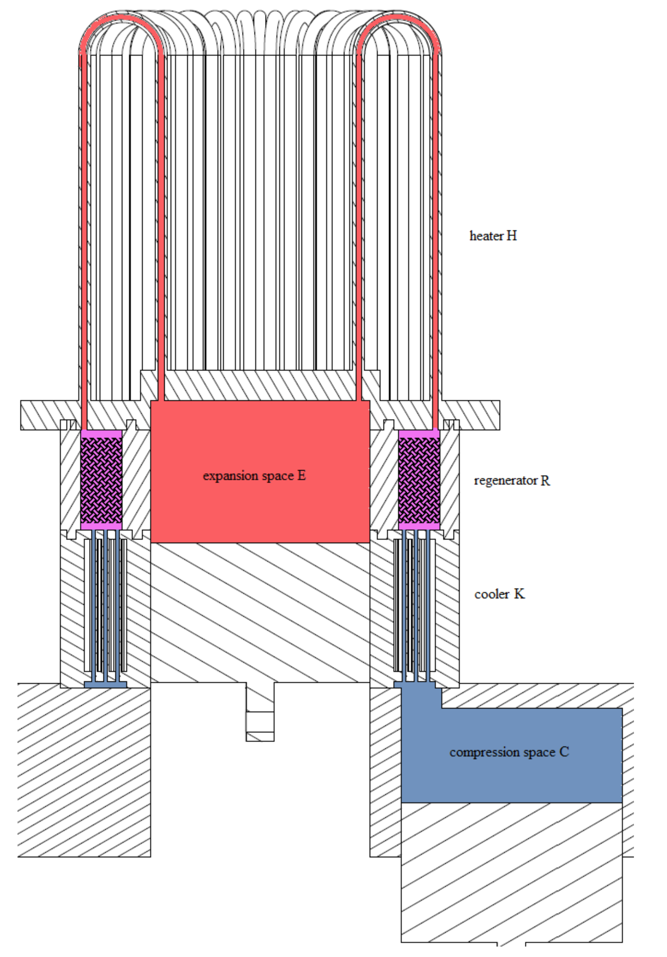
Figure 2 depicts the engine. In this figure, a section of the components is shown. The spaces that define the compression and expansion cylinders appear in blue and red, respectively.
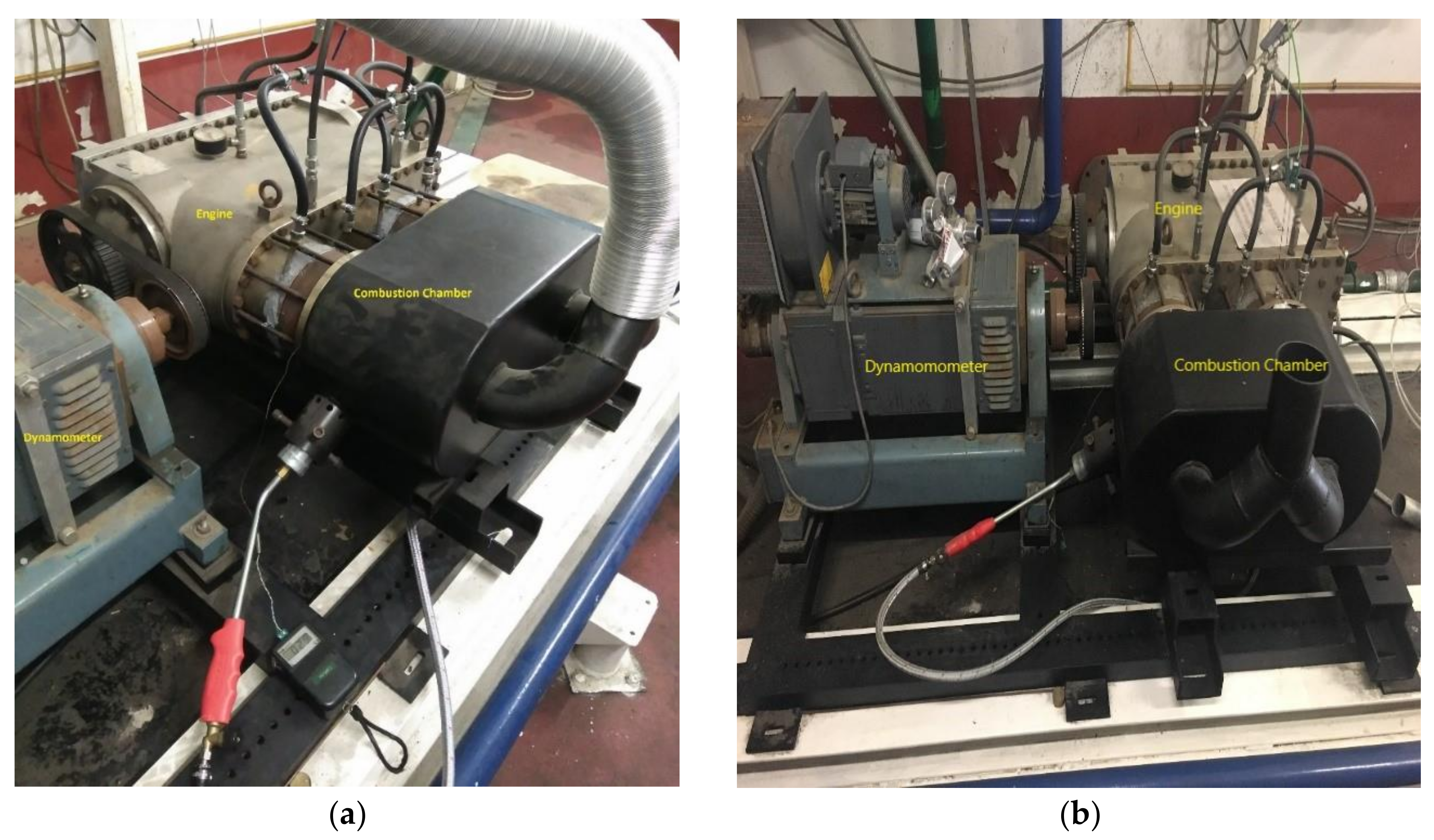
The experimental part of this paper is based on the tests on the Genoa 03 Stirling Engine (
Figure 3). The original engine was modified to adapt it to experimental installation, and to control the performance with different operative conditions of engine speed and full load. The main characteristics of the engine are shown in
Table 1, and the experimental installation is represented in
Figure 3. According to the manufacturer’s specifications, the effective power output for the engine is close to 2.9 kW when air is used as working fluid, at 600 rpm rotational speed, heater wall temperature around 750 °C, and cooler wall temperature 20 °C as cooling fluid (
Table 1). The heat exchanger materials can withstand higher temperatures, making the engine suitable for coupling to systems such as boilers based on biomass combustion. However, the engine must operate for around 5000 h to overcome the internal friction, and an initial impulse through a direct current voltage source should be provided to the flywheel during this period.
3. Numerical Model
In this section, numerical models are developed to evaluate the operating conditions of the engine. In increasing order of complexity and approximation to real behavior, the models are: the ideal isothermal model, the ideal adiabatic model, and the real adiabatic model.
In addition to these models, another model based on the adiabatic model was developed that considers heat transfer and load losses in the exchangers of the engine. This model is called a simple adiabatic model.
3.1. Ideal Isothermal Model
The ideal isotherm model was based on the model developed by Schmidt, who was the first to thermodynamically model the Stirling cycle [
14,
29]. The behavior of the working fluid in the compression and expansion cylinders is considered isothermal, which eliminates the complexity associated with the temperature variations in those cylinders.
The main assumptions of this model are: (1) the pressure has the same value in any component of the motor for the same moment of time, that is, the missing loads are neglected; (2) the temperatures in the compression and expansion cylinders are constant; (3) the mass of the working fluid is constant, meaning the gas leaks out of the engine are negligible; (4) the behavior of the working fluid is considered according to an ideal gas; (5) the speed is constant; (6) the system is considered a permanent cyclic system, meaning there are no dynamic variations between one cycle and the next; (7) variations in kinetic and potential energy are neglected; and (8) the volume variations in the engine workspaces are sinusoidal.
This model offers several advantages. Firstly, considerations such as the sinusoidal volume variation simplify the formulation of the equations to algebraic relationships, making their calculation analytically workable. Secondly, the indicated work calculated from the P-V diagram (pressure vs. volume diagram) is quite accurate.
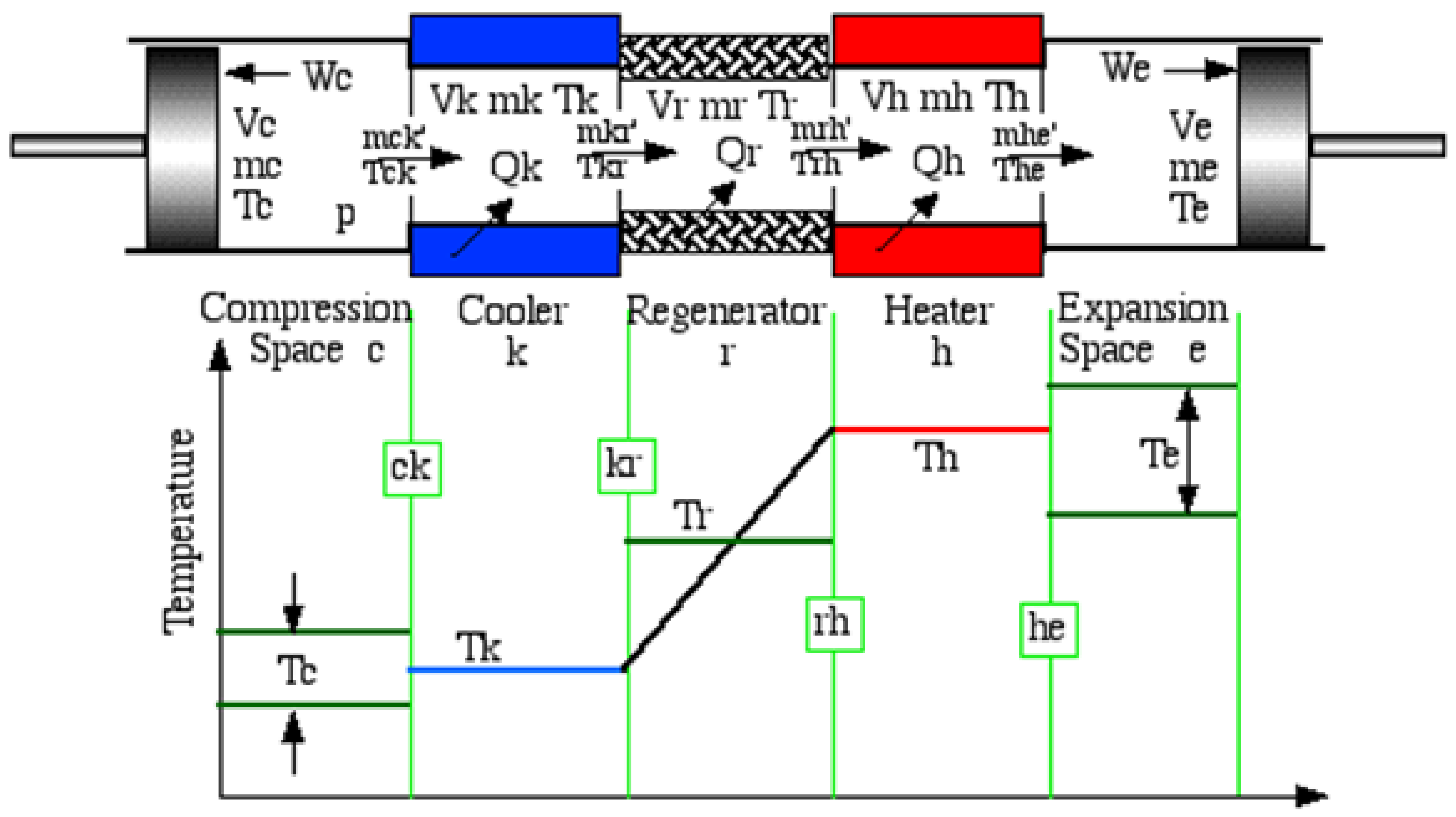
However, Schmidt’s analysis is not able to accurately determine the heat fluxes throughout the cycle, which affect efficiency. That is why the efficiency calculated with this pattern coincides with the Carnot efficiency because the compression and expansion spaces are considered isothermal, and exchangers are considered ideal, so the model has maximum efficiency. Given these considerations, the temperatures of each component of the isothermal model are represented in
Figure 4.
Figure 4 shows that the temperature of the regenerator is considered linear. In addition, the temperature in the cooler and in the heater is constant and equal to
Tk and
Th, respectively. The model consists of five components, which are connected in series. Each component is characterized as a homogeneous body with mass
m, temperature
T, volume
V, and pressure
p, which are instantaneous.
In the equations, the subscript represents the component to which it refers: compression cylinder c cooler K, regenerator r, heater h, and expansion cylinder e.
3.2. Ideal Isothermal Model Equations
The conservation equations of mass and energy are considered here and its variation is considered with the crank angle. The total mass of the system
M is the sum of all component masses
m, which is considered constant over time and with the crank angle:
Since the behavior of the gas is considered ideal, the total mass is defined by:
The effective temperature in the regenerator is necessary, and it is calculated as the logarithmic average of the temperatures in cooler and heater:
Considering the volume variations
Vc and
Ve, isolating the pressure
p as a function of these volume variations is possible:
Therefore, the work done by the system in a complete cycle is expressed by the cyclic integral of
pdV:
Volumes
Vc and
Ve vary over time depending on the position of the piston in the cylinder. In an alpha-type configuration, the phase angle between the expansion and compression volume variations is
α = π/2. Equation (6) represents the compression and expansion cylinder volume variation with crank angle, where
Vm is the clearance volume of each cylinder,
Acyl is the cylinder area,
d is the bore,
r is the crank, and
l is the connecting rod length.
Figure 5 provides a schematic of the geometric system used in the mathematical equations.
As well as the total mass of the system, the total volume of the system is the sum of the volumes of each component, so Equation (7) is:
Since the volumes Vc and Ve vary with the crankshaft angle, the total volume of the system and the pressure in the engine also vary with this angle, as this angle is the only variable independent of the set of equations.
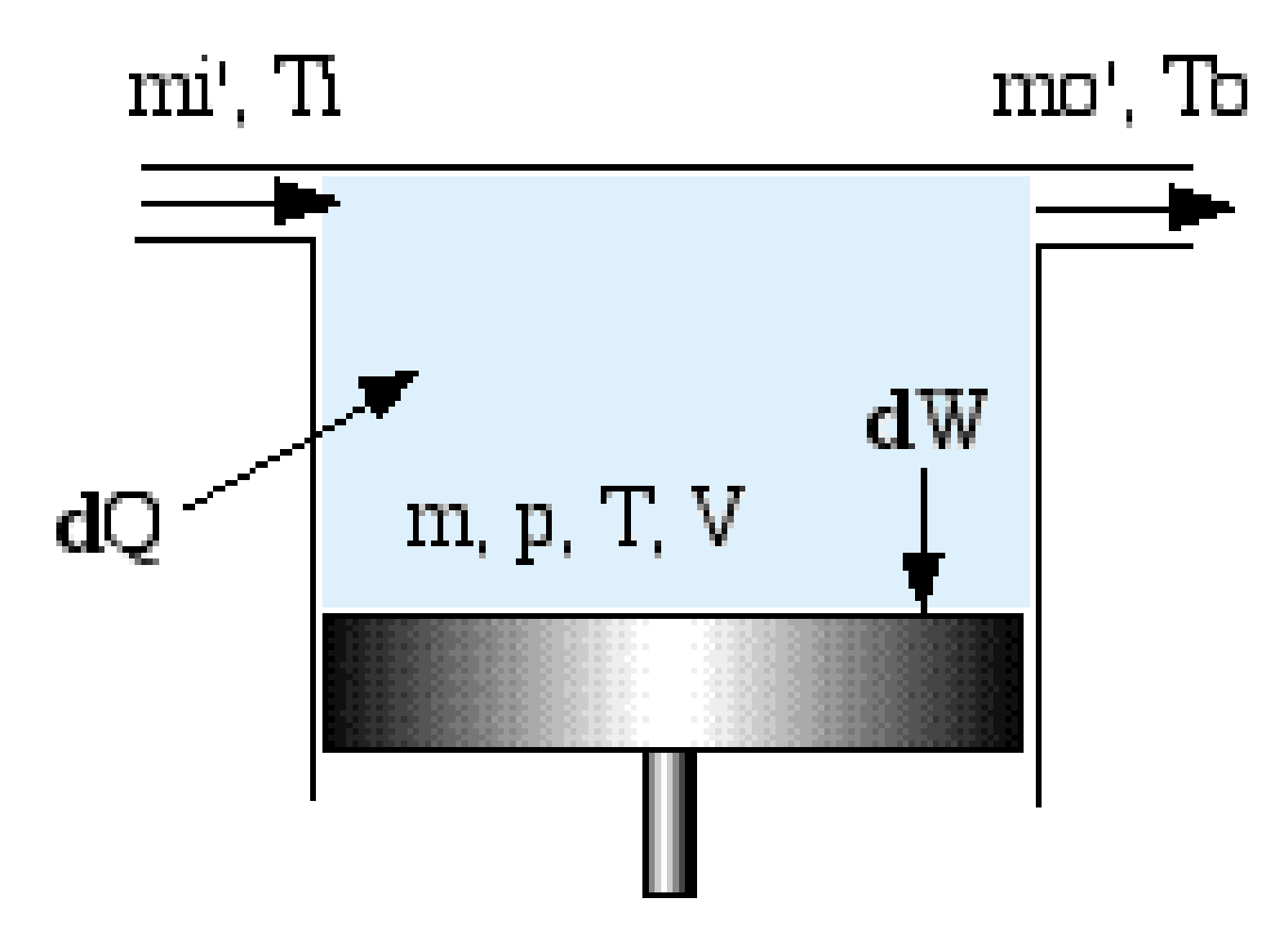
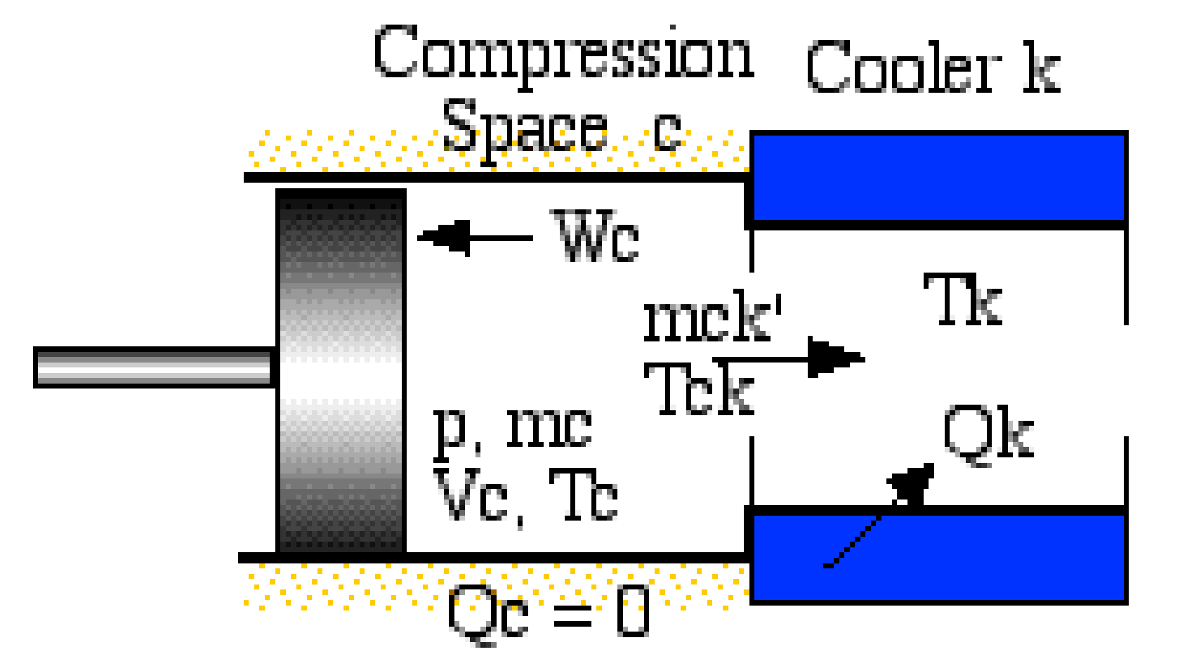
The first principle of thermodynamics was applied to each component of the engine. Considering the ideal isothermal model in terms of energy flow, the energy equation for a generic engine cell is obtained, indifferently a heat exchange cell or work, in which, in addition to the energy exchange with the outside, there is a mass flow of input and output, as shown in
Figure 6.
The enthalpy in this particular cell is determined by the difference between mass flow and inlet temperatures (
mi and
Ti, respectively) and output (
mo and
To, respectively), whereas the heat or work flows are represented by
dQ and
dW, respectively (
Figure 6). Therefore, the energy balance remains in the expression: Heat supply + net enthalpy = work in the cell + increase of internal energy.
For an ideal gas, enthalpy and internal energy depend only on the temperature, then specific enthalpy and specific internal energy can be expressed as
and
, respectively. Then the energy balance [
28] is represented by:
This expression corresponds to the classical form of the energy equation for non-stationary flow, whose terms of potential energy and kinetic energy have been neglected. Considering an isothermal model, the inlet and outlet temperatures are the same (
Ti =
To), and considering conservation of mass, the difference between the two is equal to the differential of mass in the cell, simplifying the previous equation as:
Assuming an ideal gas, the gas constant is
R =
Cp – Cv. Then, the energy balance is represented by:
Finally, the heat transferred to the gas during the cycle is obtained from the integration of
dQ. However, the hypothesis of permanent cyclical system implies a cyclical variation of the null mass throughout the cycle, for all the cells. By integrating, the following are obtained:
The above considerations lead to these results: (1) the heat transferred or absorbed by the gas is entirely turned into work in the compression and expansion spaces; (2) the net heat rate of the regenerator is zero, due to the regenerator being ideal; and (3) there is no heat transfer between the gas and the environment in the heater or cooler.
The last consideration makes the hot and cold exchangers seemingly useless pieces in this model, since the supply and transfer of heat occurs in the spaces of expansion and compression. This contradiction is a direct consequence of the hypothesis of the isothermal model of maintaining expansion and compression spaces at the same temperature as their associated heat exchangers (heater and cooler, respectively), which is an incorrect assumption.
In real machines, the ideal case tends to consider the spaces where gas energy is transformed into work, as adiabatic domains and not isothermal, which implies that the net heat of the cycle must be provided by the exchangers.
3.3. Numerical Simulation and Results
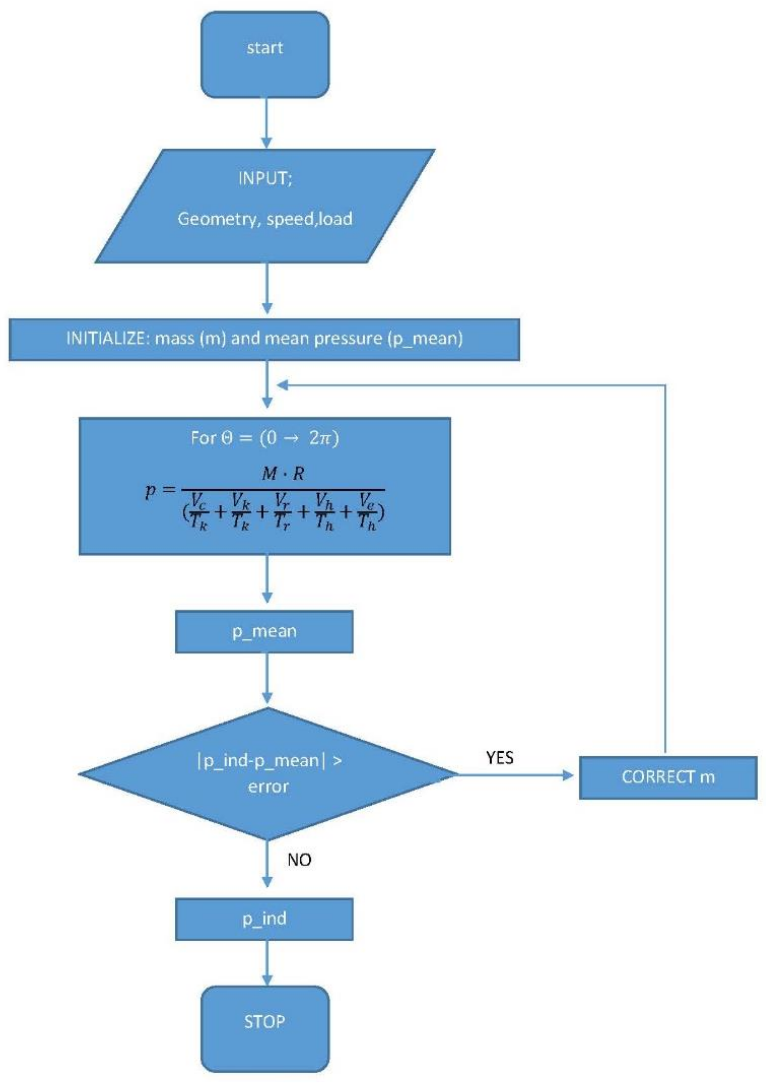
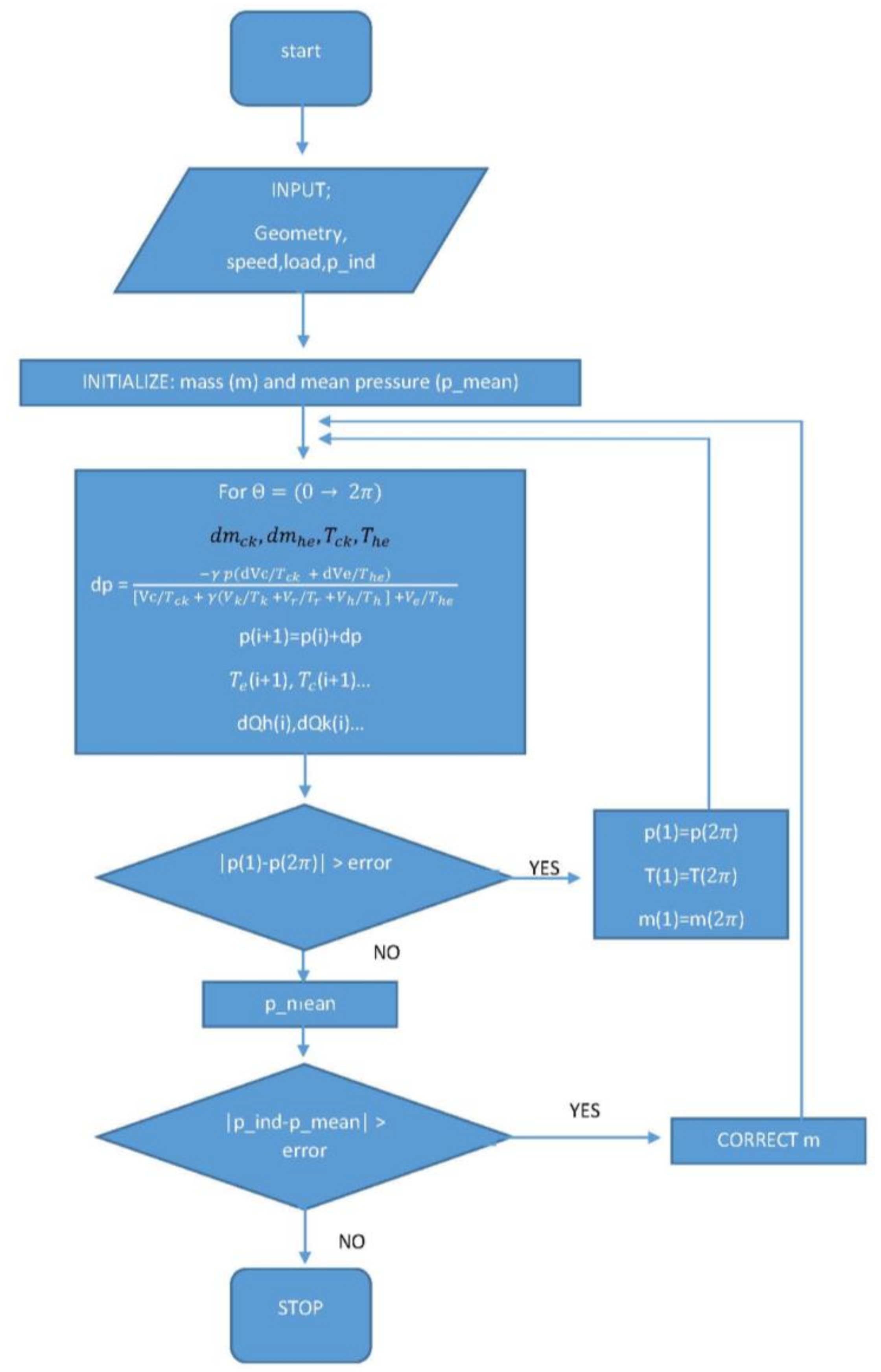
Once the engine was geometrically characterized and its boundary conditions defined, the isothermal model was simple to implement. Noting the flow diagram in
Figure 7, the model incorporates a total mass of the initial engine m, and an effective average pressure
p. Then, the code calculates the total average pressure for each value of
θ as a function of the initialized mass (
p mean) and compares it with the reference pressure. If the difference between the two is greater than the manageable error, the code enters the iteration loop correcting the mass, until convergence. Then the indicated work of the cycle can be obtained.
The total mass value of air is obtained from the simulation, once the convergence criteria is reached:
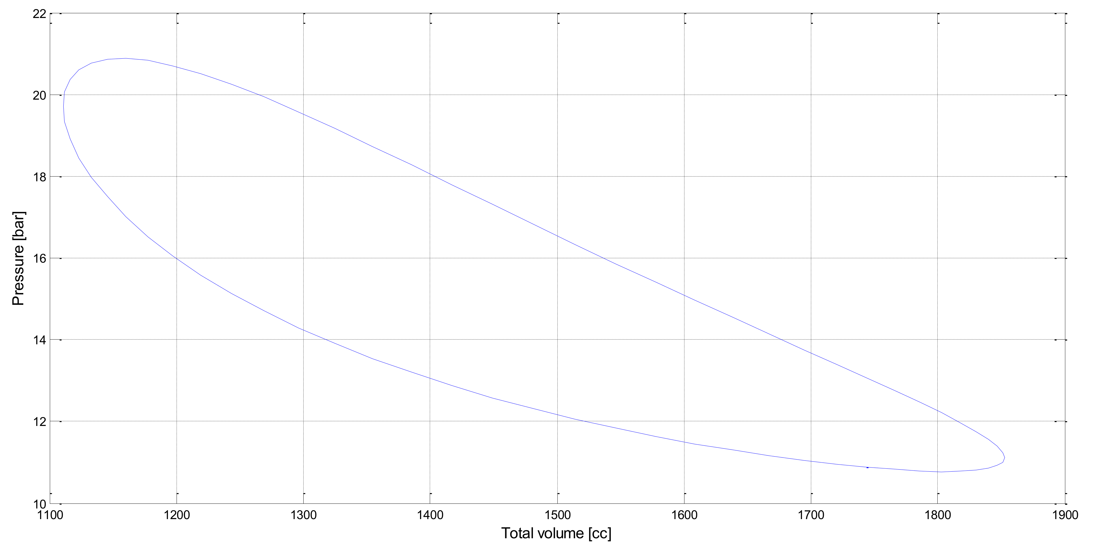
Figure 8 represents the instantaneous pressure versus volume.
The indicated work of the cycle is obtained by integrating the area of this P-V diagram. Other interesting results from the GENOA 03 simulation are as follows. The energy transfer in the heater is versus the transfer in the cooler . The work of the isothermal model is and the efficiency .
As expected, the performance matches the ideal Carnot value. Since the work and the speed are known, the indicated power of the cycle for both cylinders are calculated as
4. Ideal Adiabatic Model
This model is based on the work of Urieli [
30], who developed the adiabatic analysis for the Stirling engine as part of his doctoral thesis, and the work of Finkelstein, who first defined adiabatic work space models in air engines. The adiabatic analysis is similar to the Schmidt model in its approach, with the main exception that it considers the working fluid in the compression and expansion cylinders undergoing an adiabatic instead of an isothermal process.
Therefore, an ideal adiabatic model represents the maximum efficiency. This value is quite similar to the real efficiency value high performance engines. Therefore, an analysis of a Stirling engine must use at least the adiabatic model to ensure that the results of the simulations are useful for analysis.
Regarding the isothermal model, the rest of the hypotheses and considerations are maintained, as well as the simplification of the engine into five components in series. Certain variables must be added to the original formulation concerning to the heat exchangers in the adiabatic model, as can be seen in the schematic form of the model in
Figure 9.
The four interfaces associated with the five components of the engine must be included in this model, since the temperature between the workspaces and the exchangers are not constant in a cycle, as was the case in the isothermal model. Each interface is distinguished according to the following sub-indices: ck, between the compression cylinder and the cooler; kr, between cooler and regenerator; rh, between regenerator and heater; and between the heater and the expansion cylinder. For example, mck represents the mass flow between the compression cylinder and the cooler.
Regarding the temperatures in the cylinders, Te and Tc are calculated through the equation of the gases, known mass volume and pressure in each point, which oscillate sinusoidally. The temperature of the regenerator is now considered linear, varying between the extremes of Tk and Th. We assumed that in the cooler and heater, the temperature remains constant and equal to Tk and Th, respectively, regardless of flow direction. This consideration causes strong thermal discontinuities in the ck and he interfaces due to the simplifications of the model. However, the temperatures at the interfaces depend on the direction of flow, where a positive value of mass flow implies displacement from the compression space in the direction of expansion and vice versa. Such a condition is signified in the algorithm as:
In summary, the hypotheses and simplifications carried out by Urieli and Finkelstein were: (1) the compression and expansion spaces are adiabatic, meaning the heat exchanged between the cylinders and the environment is zero; (2) gas leaks into the environment are negligible; (3) the pressure at an instant of time is the same throughout the entire engine, and losses of load are not considered; (4) the movement of the piston-connecting rod-crankshaft chain follows the sinusoidal law described in the isothermal model (
Figure 5); (5) the heat transfer in the exchangers is considered good enough to maintain the temperatures
TK and
TH and the volume
VK and
VH of the gas, constant in its passage through the cooler and heater, respectively; and (6) the performance of the regenerator is assumed to be sufficient to maintain a linear distribution of temperature along its length, with the temperature
TK for the face in contact with the cooler and
TH for the side of the heater.
4.1. Development of Equations
The set of equations of the model is based on the solution of the differential of pressure and the differential of mass per element that occurs for an increase in the angle of rotation of the crankshaft. The differential shape of mass conservation, amount of movement, and conservation of energy in expansion and compression spaces are used, in addition to the state equations applied to the exchangers.
Firstly, the differential conservation of the mass in Equation (11) provides:
Similar to the isothermal model, the behavior of the gas is considered to be ideal gas. This hypothesis is close to the real behavior, since the gas is found in conditions far from the critical point.
Deriving the form of the law of ideal gases for pressures, and knowing that throughout the cycle the temperatures and volumes in the exchangers are constant, we obtain:
Equation (13) is obtained by substituting the differential form of conservation of mass into the equation of state:
The intended objective in the isothermal formulation is to obtain a relationship for the pressure differential depending only on the independent variable, in this case, the angle
θ. Then, it is necessary to clear the terms
dmC and
dme.
Figure 10 is a diagram of the variables and flows in the compression cylinder. Applying the energy balance to this control volume, Equation (14) is obtained:
The compression is adiabatic, then
dQc = 0, and the work is defined by
dWc =
pdVc. The differential mass
dmc is equal to the mass flow through the interface
CK,
mck, reducing the equation to:
By substituting the equation of state and ideal gas relationships, an expression of the differential mass as a function of pressure is obtained. This relationship can be expressed as Equation (16), analogous for both the compression space and the expansion space:
Finally, the differential pressure for each instant of the cycle is defined by:
The equations associated with dp and dm pose a system of differential equations with several unknowns associated with the temperatures Tc and Te and the masses mc and me. As the resulting system is non-linear, it can only be solved by numerical integration, as a problem of initial values associated with an iterative process defined by certain convergence parameters.
Once
p and
m have been evaluated, the rest of the variables can be obtained through mass balance and state equations. The parameters
dVc,
dVe,
Vc, and
Ve are easily calculated by the kinematics relationships. The differential equations of the temperature in the workspaces are derived from the ideal gas equation:
The indicated work of the cycle is the sum of the work done by each cylinder:
Through the energy equation, and replacing the values of
dT and
dW, a more adequate form of that equation is obtained, which is easily applicable to each component:
For example, for the three exchangers, where there is no work exchange and the volume is constant, Equation (21) is obtained by reducing the previous expression:
4.2. Solution Method
Once the system of necessary equations was established, and having characterized the motor in the development of the isothermal model, the objective was to solve the differential equations of temperature, mass, and pressure in both cylinders, to represent the distribution of these parameters in a complete cycle, and calculate the performance of the engine. In this case, the problem is non-linear and more discontinuous than in the isothermal case, since two temperatures have been incorporated conditional on the direction of flow.
Figure 11 shows the simplified flow diagram of the ideal adiabatic model and simply expresses the execution order of the solution algorithm, although some key operations are missing, such as the one related to the conditional temperatures.
The simplest solution to solve this set of differential equations is to formulate it as a problem of initial values, so that the initial values of all the variables are known, and the equations are integrated throughout the cycle, meaning the crankshaft makes one full circle. However, the adiabatic model acts more like a problem of boundary conditions and not initial values, since these values are not known in advance. If we assign initial values from the solution of the isothermal model, it is possible to integrate the equations from these values. After several iterations of the complete cycle, the condition that establishes that the values of the variables at the end of the cycle (2π) and at the beginning of the cycle (0) coincide, which is the condition of reaching the permanent cyclical system of the cycle.
Once the convergence in the previous condition was obtained, the next step was to satisfy the operating conditions, so that the average pressure of the cycle coincides with the design pressure. For this purpose, an iteration loop is required. With the considerations set out above, the algorithm was sufficiently stable to generate the convergence of the solution by changing parameters, such as the motor geometry or the operating conditions of the motor, in a range close to the design point.
4.3. Numerical Simulation and Results
The solution for the adiabatic model was obtained, where the temperature distribution,
Te and
Tc, are variable with time, and the distribution of energy flows through each component.
Figure 12 represents the temperature distribution of the adiabatic model, the compression and expansion temperatures can be observed varying throughout the cycle.
The most striking finding is that this temperature variation implies a reduction in the average temperature in the expansion cylinder. Since the oscillation has an amplitude of around 200 K, this decrease in temperature with respect to the adiabatic model will be reflected in the thermal performance of the machine, which will no longer be equivalent to the ideal Carnot performance, yielding a much more realistic ideal value.
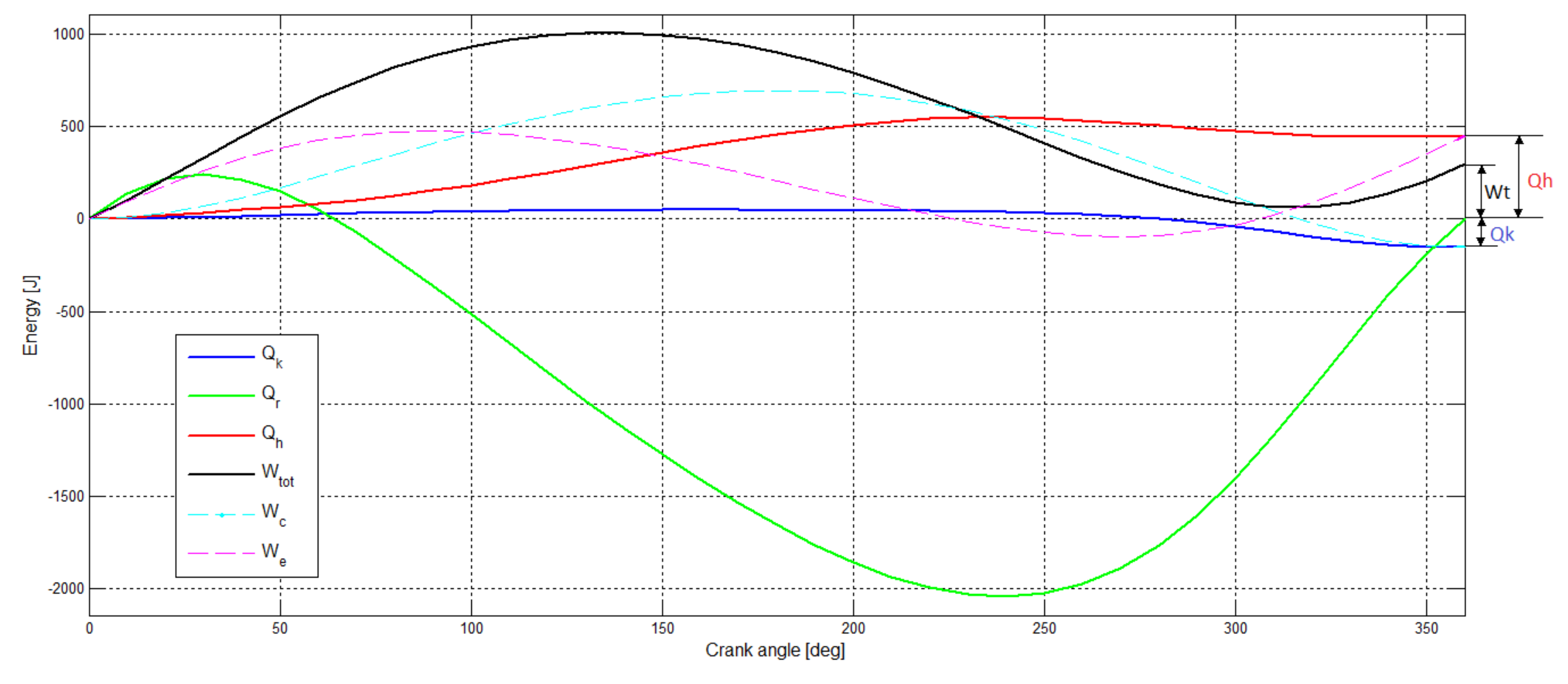
Regarding the energy flows along the motor,
Figure 13 shows that the values relative to the heat flow in the exchangers next to the values of the net work, appear to overlap. This diagram provides valuable information on the behavior of the ideal adiabatic model. The integral of the curve does not correspond to the net value of each parameter, but the value for each point of the curve is the accumulated net value, zero at the beginning of the cycle, (reference), and the net value for a complete cycle at the point
θ = 360°. With regard to work, those components associated with the compression and expansion spaces appear, and the net work, which is the sum of both values, where the net work of expansion is positive, and that of compression is negative.
The heat flow of the regenerator is zero at the end of the cycle, since we considered it to be ideal in this model. However, throughout the cycle, energy values in the order of 10 times the final net work are produced, which implies that the regenerator is a key element in the design of the engine, since the performance in a non-ideal case depends crucially on the capacity of the component to absorb and yield large heat flows.
The exchangers produce a net value identical to the value of the associated work volume:
Qh =
We and
Qk =
Wc. This is a strange result and reveals one of the aspects that the adiabatic model models incorrectly. The key to this phenomenon is in the regenerator, which, being ideal, behaves like perfect insulation between the cold and hot areas of the engine, so that the energy balance in each part equals the work in the corresponding heat flows. These net flows of heat and work are qualitatively represented in the right margin of
Figure 13.
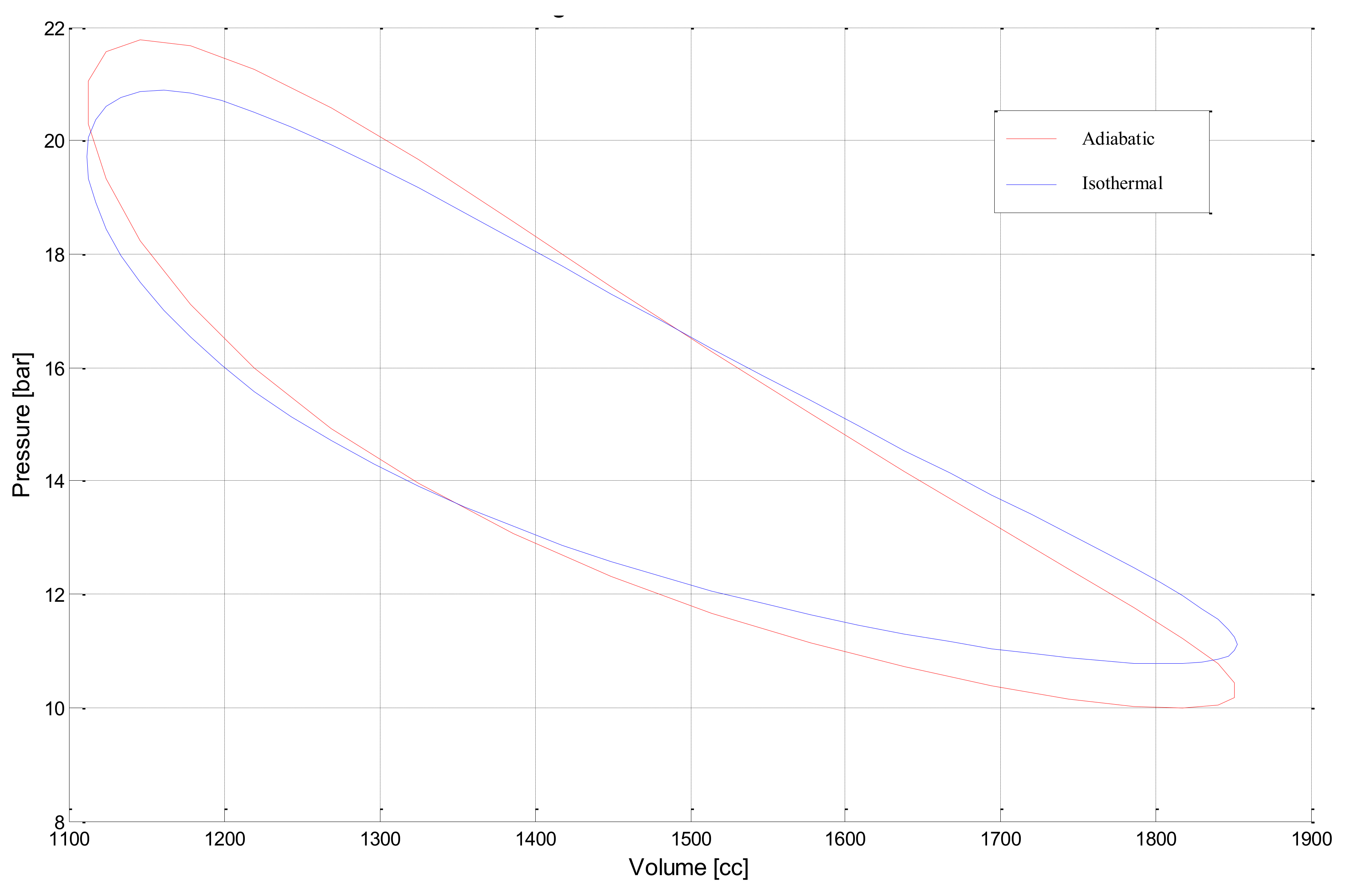
Figure 14 is a diagram is superimposed on the P-V diagram of the isothermal model. Both diagrams are similar, where the efficiency and power of the adiabatic model are only 10% less than the isothermal values. We must not forget that both are ideal models. One of its main advantages is the precision of the solution at engine pressures.
By integrating the area of the P-V diagram of
Figure 14 for the adiabatic model, the indicated work of the cycle is finally obtained. In addition, analogously to the adiabatical model, the heat flows and the thermal efficiency of the GENOA 03 engine are
in the heater versus
in the cooler. The work of the adiabatic model is and the efficiency is
.
The power, calculated using the same method as in the isothermal model, is kW.
We concluded that the adiabatic model is more realistic than the isothermal model; however, several of the results remained inconsistent with the real behavior of an alternative engine, especially in terms of the exchangers. As a compensatory measure, the adiabatic analysis, considering all the operative parameters and variables that it can resolve, offers a valuable information for separately understanding the operating conditions of each of its components.
In this paper, the ideal adiabatic model was an indispensable tool to understand the mass flow of air that circulates through the exchanger, the directions of the flow, that spikes of flow velocity occur at times, and reversal of flow dead points, which were all required in order to design alternatives that could be compared with each other for some boundary conditions as similar to the behavior of the real engine as possible.
In addition, the ideal adiabatic model was presented as a base to introduce modifications and auxiliary functions, in order to analyze the effectiveness of heat transfer in the exchangers, the effect of including the geometry of the motor with interconnections among elements, or load losses, by means of air friction on the motor walls.
5. The Simple Model
The next step was to design a new model based on the adiabatic model that is capable of evaluating changes in engine performance by modifying or changing components, such as exchangers, or is more precise when defining boundary conditions, for example, defining a cooling water flow at a certain temperature instead of imposing a temperature on the internal wall of the cooler. The model developed below adds functions and calculation aspects complementary to the adiabatic model, which is called the simple model. This model, in some references, is still labelled adiabatic [
29], although the original algorithm of the ideal model has been modified, and some intermediate control variables have been added. However, the solution procedure is essentially the same, and the spaces of compression and expansion walls are still considered adiabatic.
As this model is modified into more than a numerical model, the procedure to follow depends on the literature that was consulted, as many projects on Stirling engines, like this one, use modifications of the ideal adiabatic model. Urieli [
30] produced one of these models, which we followed in this study. This approach adds three fundamental aspects: the heat transfer distinguishing the regenerator from the other two exchangers, the flow friction losses in the three exchangers of the engine, and their influence on the performance of the engine.
The efficiency of the regenerator was assumed to not be ideal when studying the influence of this parameter on the engine performance. The heat transfer in the cooler and heater was evaluated by means of the forced correlations convection for the transfer between the working fluid and the exchanger walls, so that a wall temperature for each exchanger was assumed. The flow friction, also called load of losses, refers to the mechanical work required to pump the working fluid through the exchangers. This mechanical work must be provided by the indicated cycle work by reducing the net power of the engine.
Once the model simultaneously implements these three aspects, the numerical simulation was carried out for the GENOA 03 engine, and was contrasted with the ideal models.
5.1. Characterization of the Non-Ideal Regenerator
As discussed above, the regenerator of a Stirling engine is a key component critically influencing engine performance. However, throughout the history of the Stirling engine, the operation theories of this component have been based on hypotheses supported only by experimental studies, extrapolated from a configuration or other models [
29,
31]. The regenerator is a device that works cyclically in the direction of flow. The hot air flows from the heater, transfers part of its heat to the regenerator mesh, and the mesh transfers as much of the heat absorbed into the cold air from the cooler as possible. In steady state, therefore, the net heat transfer of the regenerator is zero. The effectiveness of the regenerator is usually expressed as the ratio of the enthalpy variations in the real flow with respect to the maximum theoretical variation in an ideal regenerator. However, to adapt to the simple model, which we consider the ideal case, we defined efficiency ε as heat transferred between the mesh and the gas in a single pass through divided by heat transferred in the regenerator of the ideal adiabatic model.
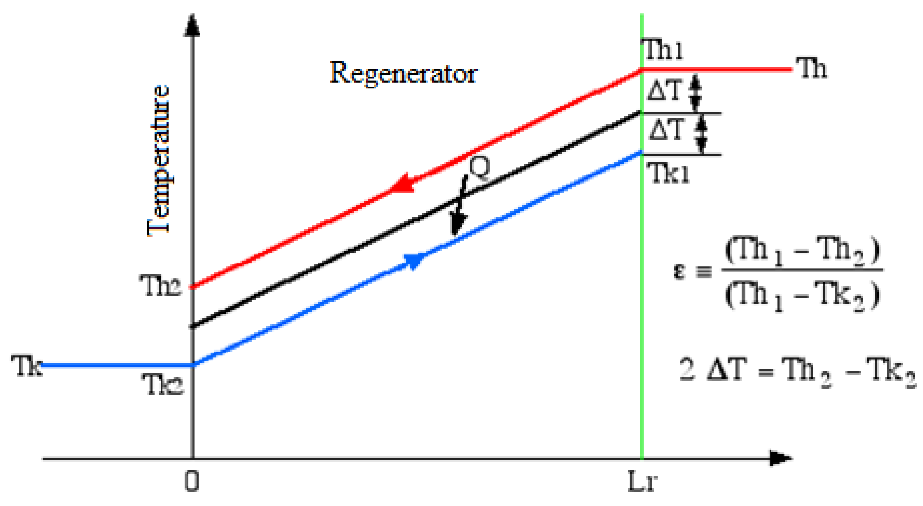
Figure 15 represents the temperature evolution of both flow diagrams through the regenerator if they are not ideal.
We assumed that the variation between temperatures ∆
T, and cold and hot input and output were identical at both ends of the regenerator. From
Figure 12, the efficiency in terms of temperature can be expressed as:
where
ε = 1 for the ideal regenerator, and
ε = 0 means there is no regenerative effect. To assess the effect of these variations on cycle performance, we started from the general expression of thermal efficiency for the ideal model (with superscript ‘):
For the non-ideal case, the heat exchanged by the cooler and heater is the ideal value plus the sum of the heat that the regenerator has not been able to absorb:
Substituting the values of
QH,
QK, and the ideal efficiency
ηi in the equation of the non-ideal thermal efficiency we obtain:
Knowing the thermal efficiency and the ratio between the heat of the regenerator and the heater in the ideal case, a proportional relationship between the efficiency of the regenerator and the non-ideal thermal efficiency can be expressed. As such, we observed that by varying the efficiency in its absolute range, if ε = 0, the thermal efficiency falls from the ideal case ≈ 65% to values around 10%.
Low efficiency values, e.g., 80%, have various implications for the engine. The overall efficiency can drop up to 30%, and if the regenerator is not able to remove a considerable part of the heat energy, the cooler must be larger, increasing the load losses and decreasing the net work.
5.2. Characterization of Heat Exchangers
The model used to characterize these heat exchangers was analogous for both components, using basic equations and correlations of heat transfer in forced convection. In this model, we assumed a constant wall temperature
Tw, together with an average mass temperature of the air through the exchanger, where we only considered the forced convection of the air through the tubes, and we did not consider the convective exchange with the external water or the conduction through the tube walls, as shown in
Figure 16.
The efficiency of the exchangers [
32] could be evaluated in advance using the
ε-NTU method (effectiveness—number of transfer units method), but to do so, a more complete analysis that the one proposed by the simple model is needed. In
Section 5, the
ε-NTU method is implemented as a cooler analysis tool. For the present case, we started from a wall temperature
Tw related to the average temperature of mass
T using the convection equation:
where
Q’ represents the heat energy,
AW refers to the wetting area of the exchangers, and
h is the convective coefficient. To evaluate this equation in terms of heat per cycle, it was necessary to divide by the machine frequency,
f (Hz) or (s
–1). We expressed the values of
Qk and
Qh as shown in Equation (27):
The pair of equations on the right are the ones that finally implement the simple model code. We observed that by distinguishing between wall temperature and gas temperature, we defined some losses by transference. This, added to the already mentioned losses by efficiency of the regenerator, brings the model even closer to the real case.
5.3. Characterization of Load Losses
Throughout the previous models, we assumed that the pressure remained constant throughout all components of the engine at the same time. However, the passage of the flow through heat exchangers, in this case, banks of tubes, and through a mesh in the case of the regenerator, generates considerable friction due to the fluid on the walls of these components, which is a phenomenon that must be considered in a more advanced model. These friction losses are generally called load losses, expressed in units of pressure. They directly influence the expression of the indicated cycle work, which, as stated above, depends on the integration of pressure and volume in the engine workspaces, where load losses decrease the final net work.
To quantify these losses, we proceeded from the expression of the indicated work and added a term of pressure loss summation in the three exchangers ∑∆
p at the end of the pressure at one of the engine ends, obtaining:
By moving the terms of the previous expression, the initial indicated work can be expressed on one side and the load losses Δ
W on the other:
To characterize these pressure losses in each exchanger, following the procedure described by Kakaç [
31], losses within a circular duct are influenced by the fluid velocity, the density, the roughness of the tube walls, and tube diameter and length.
Expressing the previous relationships as a dimensionless set of parameters, Equation (30) is obtained:
where
f is the Fanning friction factor, a dimensionless parameter related to the shear stress that the wall induces on the flow. This factor for turbulent flow is determined by experimental correlations, depending on the Reynolds dimensionless number, or by Moody’s abacus [
32].
For its implementation in numerical models, it is more appropriate to use numerically expressible correlations, such as that introduced by Drew et al. [
32], applicable to simple pipe geometry:
Finally, the expression of the load losses in a pipe remains as:
5.4. Numerical Simulation and Results
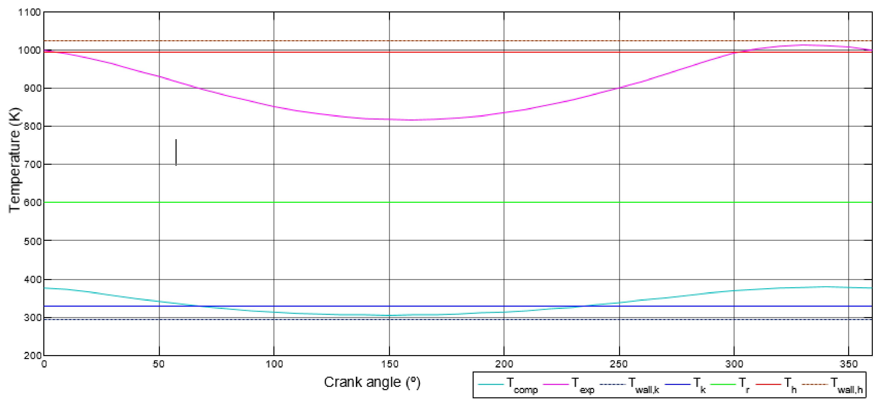
The solution procedure and the convergence criteria are identical to those of the ideal adiabatic model, with the exception that the temperatures
Tk and
Th are now values that must be found after an iterative process, based on the wall temperatures
(Twall, K and
Twall, H), and be incorporated into the equations of the previous model. As the range between temperatures decreases to about 60 °C in total, the thermal efficiency falls 5% with respect to the ideal adiabatic model. The distribution of temperatures remains as shown in
Figure 17.
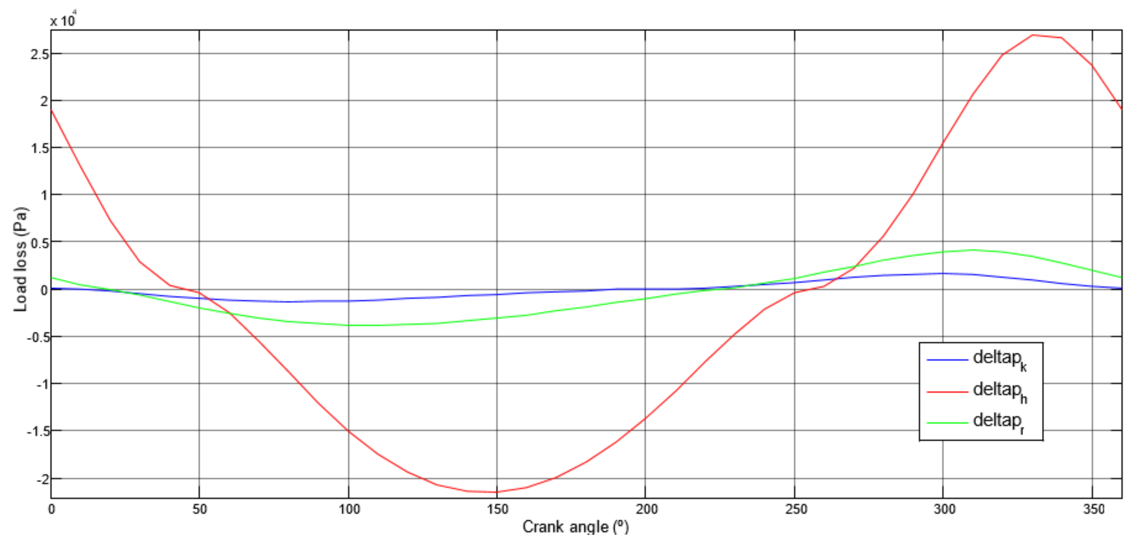
The load losses shown in
Figure 18 were analyzed with regard to two aspects. The first involved separately analyzing the distribution of the load losses of each element. In
Figure 18,
deltapk,
deltaph and
deltapr are the load loss of the cooler, heater and regenerator, respectively.
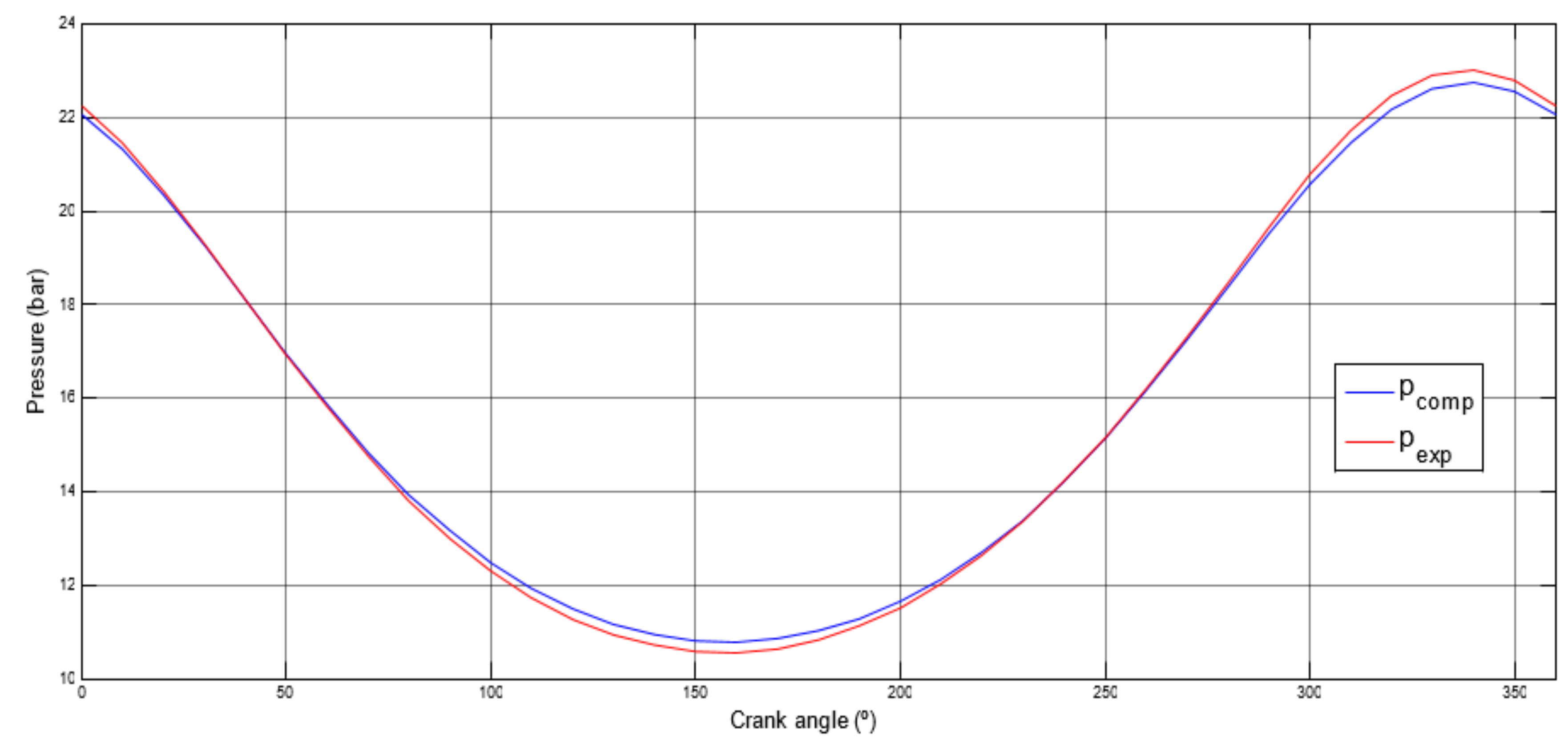
Figure 18 shows how the heater’s load losses are almost six times greater than in the regenerator. This has a simple explanation if we consider the enormous length of the heater compared to the length of the cooler or regenerator. As the load losses linearly depend on the length of a conduit, this result seems logical, even considering that the regenerator consists of a compacted mesh; the length in the heater is a parameter of greater weight in this case. The second aspect was observing the difference in the pressure distribution of the compression cylinder (
pcomp) with respect to the expansion cylinder (
pexp) once the losses in the code were implemented (
Figure 19). The difference between the two pressures represents the load losses.
To provide an idea of the importance of the load losses, the previous pressure distribution implies a friction loss of 16.6 J, which represents 6% of the indicated work without losses, producing an indicated work cycle of 257.5 J.
As in the previous sections, the mean values of the simulation of the simple model are the heat flow in the heater versus in the cooler. The simple work is and the efficiency is. The power, calculated using the same method as in the simple model, is kW.
The combined effect of the pressure losses and the increase in heat demand, considering a non-ideal regenerator and the wall temperatures, drastically reduces the thermal efficiency related to the previous models, with a decrease of more than 20% compared to the adiabatic case.

 ,
, 


