An Anti-Islanding Protection Technique Using a Wavelet Packet Transform and a Probabilistic Neural Network

Abstract

This paper proposes a new islanding detection technique based on the combination of a wavelet packet transform (WPT) and a probabilistic neural network (PNN) for grid-tied photovoltaic systems. The point of common coupling (PCC) voltage is measured and processed by the WPT to find the normalized Shannon entropy (NSE) and the normalized logarithmic energy entropy (NLEE). Subsequently, the yield feature vectors are fed to the PNN classifier to classify the disturbances. The PNN is trained with different spread factors to obtain better classification accuracy. For the best performance of the proposed method, the precise analysis is done for the selection of the type of input data for the PNN, the type of mother wavelet, and the required transform level which is based on the accuracy, simplicity, specificity, speed, and cost parameters. The results show that, by using normalized Shannon entropy and the normalized logarithmic energy entropy, not only it offers simplicity, specificity and reduced costs, it also has better accuracy compared to other smart and passive methods. Based on the results, the proposed islanding detection technique is highly accurate and does not mal-operate during islanding and non-islanding events.

1. Introduction

The rapid growth of energy demand in recent years has contributed to the popularity of the utilization of renewable energy. The environmental and economic benefits of renewable resources e.g., photovoltaic systems, wind turbines, fuel cells, and geothermal energy make them very attractive to researchers and governments around the world [1,2]. In this regard, the developed countries have been trying to reduce their levels of greenhouse gas emissions in order to address the problems of climate change and economic recovery by focusing on the energy resources. “Energy Roadmap 2050” and “Roadmap Towards a Competitive Low-carbon Economy Until 2050” from the European Commission are among the policies that have been put in place to reach the global political goal of staying below a 2 °C temperature increase [3]. In order to achieve these challenging goals, effective renewable energy resource support policies and an effort towards the improvement of energy efficiency are necessary.

One of the vital problems of these energy resources in distributed grid is an islanding phenomenon. Islanding occurs when a part of utility grid which contains loads and distributed generation (DG), separates from the rest of utility grid while this part is still energized. This can lead to serious hazards for protection devices and the safety of the grid crews [4]. Thus, islanding should be detected quickly and the system must be de-energized. Out of the aforementioned renewable sources, the solar-based power generation is one of the most popular energy resources which provides between 1.3% and 1.8% of the global electricity usage [5]. The islanding phenomenon can reveal itself in grid-tied photovoltaic systems once a part of utility grid containing the local loads and photovoltaic (PV) inverter is tripped off from the main utility grid while the local loads gets power only from the PV systems. This situation creates the most serious safety problems in photovoltaic (PV) generation as the power supply is now without control and supervision. It is expected that the magnitude of the voltage and frequency of the power system parameters will be unpredictable once the islanded system operates without utility control [6]. Thus, in order to ensure the reliable operation of grid-tied photovoltaic systems and reduce the cost of installation of such energy resources, PV inverters must include an effective and consistent anti-islanding process [7]. Hence, various existent standards have been established for grid connection systems. According to these standards, islanding conditions should be detected within 2 s and distributed generation operation must be stopped [8,9,10,11,12]. Thus, different anti-islanding detection techniques have been proposed in order to incorporate them into distributed generation (DG) operation. These methods can be divided into two main groups e.g., remote techniques, and local techniques [13,14,15,16], where the performance of each islanding detection method is evaluated based on its non-detection zone (NDZ). The main reason why islanding detection methods (IMDs) fail to detect islanding is because of the non-detection zone. The non-detection zone can be a good criterion in islanding detection control techniques [17,18]. The communication or the remote technique is based on communication between the utility grid and energy resources. In spite of its better performance, the high cost and complexity of remote techniques may eventually pose a barrier to their application, especially for small distribution networks [19]. Some common remote islanding detection schemes are listed in [19]. Instead of using remote techniques, local measurement-based passive and active methods are utilized. The active methods are based on the injection of a small perturbation at the distributed generation (DG) inverter output and examining the variation in output parameters to detect the islanding. In spite of its capabilities in reducing and or even eliminating the NZD, it causes a large degradation of the power quality of the network, high functioning time, and increases the complexity of the system due to the additional controllers/power electronics equipment needed [17,18]. A comprehensive survey on active detection techniques can be found in [17,18,19,20,21,22]. The mainstream methods are passive methods, which are based on measuring certain parameters such as voltage, frequency, current, and harmonic distortion of signals at the point of common coupling (PCC) and comparing them with a given threshold value [17]. The passive methods are moderately suitable due to their smooth execution, practical solutions and no effect on power quality [21,22,23,24,25], but they have some disadvantages such as threshold setting, large non-detection zones, high error detection rates, and low consistency in correctly detecting the islanding [22]. Over/under voltage, over/under frequency, overcurrent, voltage phase jump, rate of change of frequency, rate of change of power, and harmonic distortion schemes are the most common passive methods. Comprehensive surveys on passive islanding detection techniques are presented in [13,19]. In recent years, in order to improve the performance of passive techniques and reduce NDZ, passive methods based on the combination of soft computing with modern signal processing techniques have been applied. For example, a decision tree in combination with adaptive boosting has been proposed in order to improve the islanding detection accuracy [26]. However, the proposed method’s sensitivity to outliners and the noisy conditions is considerable [26]. Support vector machine (SVM) with wavelet transform has been utilized to detect islanding [27]. The results of the proposed method show that although as signal processing tool the wavelet transform has suitable time-frequency localization ability, it faces barriers, e.g., batch processing step, non-uniform frequency sub-bands, less flexibility and detection failure during noisy conditions [27]. Different methods based on the combination of artificial neural network and fuzzy logic are presented in [25,28,29]. A deep learning method with a hybrid wavelet transform and multi resolution singular spectrum entropy is done for a single phase photovoltaic system. The proposed technique has good performance for the test cases considered in [30]. WPT signal analysis and a back propagation neural network are applied for islanding detection of a single phase photovoltaic system [31]. Despite the previous works in this area, still there is a lack of an islanding method that is fast, reliable, easy to implement and has low computational burden.

In this work, a new islanding detection technique based on the combination of WPT and PNN is proposed to detect islanding conditions from grid faults. The strategy of the proposed method is categorized into two main parts. In the first step, the PCC voltage is measured and processed through a wavelet packet transform in order to find the normalized Shannon entropy (NSE) and normalized logarithmic energy entropy (NLEE). Then, the obtained feature vectors are fed to a PNN classifier in order to distinguish between islanding conditions and grid faults. In order to obtain the best performance of the proposed method, a precise analysis is done for the selection of the type of input data as PNN input, the type of mother wavelet, and the required transform level based on accuracy, simplicity, specificity, speed, and cost parameters. In order to train the PNN classifier, different spread factors are taken into account. Results show that the proposed method is able to detect islanding conditions even under the worst scenarios, decrease the NDZ area to zero and avoid the threshold selection. The proposed islanding detection technique is simple, easy to execute, with a quick response time, and efficient. The remainder of this paper are organized as follows: The studied model is presented in the next section. Section 3 discusses the structure of the proposed methodology. The results and discussion are presented in Section 4. Finally, the conclusions are given in Section 5.

2. Studied Model

2.1. Case Study

The studied system is a 250-kW photovoltaic array connected to a typical North American distribution grid via a three-phase converter system, as shown in Figure 1a. This system consists of a PV array, a three-phase inverter which is modeled by a PWM-controlled 3-level IGBT bridge, an inverter choke RL, a small harmonic filter C in order to filter the produced harmonics with the IGBT bridge, a step up three phase transformer 250-kV A, and 250 V/25 KV to connect the PV inverter to the grid. The utility grid consists of loads, two 25-kV feeders with lengths of 8 km and 14 km, and a grounding transformer. The utility grid is connected to the rest of system by the closed-circuit breaker SW1. There are two operation modes, namely grid connected mode and islanding mode that are controlled by the closed/opened circuit breaker SW1. The nominal frequency of the system is 60 Hz. A sample of the system data is given in the Appendix A.

Figure 1b illustrates the block diagram of the inverter controller. The inverter control system can be operated as follows: the photovoltaic voltage and current are fed to a Maximum Power Point Tracking (MPPT) controller that is based on the fuzzy logic controller to provide a DC voltage that will draw maximum power from the PV array. This control system changes the Vdc reference signal of the VDC regulator automatically so as to obtain an optimal DC voltage. The DC-link voltage (VDC metered) is compared to the DC voltage reference, and the difference between them is utilized as an input to the DC voltage regulator to determine the required $I_d$ reference for the current regulator fuzzy logic controller. In order to determine the frequency and the phase angle $\theta$, the PCC voltage $V_{PCC}$ at the point of common coupling is measured and fed to a phase-locked loop (PLL). PLL is necessary for synchronization and voltage and or current measurements. The phase angle is fed to three blocks, namely $abc \mathrm{to} dq0$ transformation, $abc \mathrm{to} dq1$ transformation, and measurement. To determine the voltages of $V_d, V_q$ and the currents $I_d, I_q$, voltage and current are measured at the PCC point and fed to a $abc \mathrm{to} dq0$ transformation and $abc \mathrm{to} dq1$ transformation, respectively. The generated current reference from the VDC regulator $\left(I_{d-ref}\right)$ is then compared with $I_d$ and the difference between them is utilized as an input to the current regulator block. The other input of this block is the difference between $I_q$ and $I_{q-ref}$. Apart from these inputs, voltages $V_d$ and $V_q$ are fed to the current regulator block directly. The output of the current control block is $V_{d-con}$ and $V_{q-con}$ which are converted to $U_q$ and $U_d$ in the measurement block. The $U_q$ and $U_d$ are fed to $abc \mathrm{to} dq$ transformation and converted into three modulating signals $\left(U_{abc-ref}\right)$ utilized by the Pulse Width Modulation (PWM) generator. The PWM generator produces firing signals to the inverter based on the required reference voltages. In order to change the 500 V—dc link voltage (VDC) to 260 AC and retain unity power factor, the voltage source control (VSC) is utilized. The VSC control system utilizes two control loops, namely an external and an internal control loop. The external control loop is utilized to regulate dc-link voltage to ±250 V whilst the internal control loop adjusts I_d and I_q grid currents. The I_d current reference is the output of the DC voltage external controller whilst the I_q current reference is set to zero to maintain a unity power factor. A sample time is used for the voltage and current controllers and phase-locked loop (PLL) synchronization unit through the control system. Pulse generators of VSC converters utilize a quick sample time so as to obtain a suitable resolution of PWM waveforms. Interested readers can find the details of the inverter control system in [32].

2.2. Non-Detection Zone

Non-detection zone (NDZ) is one of important indexes to specify the efficiency of islanding detection methods. Indeed, NDZ is an operating area in terms of imbalance of power between local generation and local loads which cause malfunction relays to identify islanding conditions. In this work, NDZ is specified by an Over/Under voltage protection relay (OVP/UVP) and Over/Under frequency protection relay (OFP/UFP) scheme [33]. This scheme is used for constant current inverters. The active power mismatch is calculated as follows [33,34]:

∆P = −3V × ∆V × I

(1)

where ∆P and ∆V are the active power mismatch and voltage deviation. V indicates the rated voltage and I is the rated current. With respect to an acceptable voltage range in a distributed grid (V_min = 0.88 pu to V_max = 1.1 pu), the level of voltage is equivalent to ∆V = −0.12 pu and ∆V = 0.1 pu, respectively. The imbalance values from (1) for the system under study, are 30 kW and −25 kW, respectively. The NDZ of the reactive power is calculated by the equation below [34]:

$$\Delta Q=3\frac{V^2}{{\omega }_{n}L}(1-\frac{f_n^2}{{\left(f_n\pm \Delta f\right)}^2})$$

(2)

where $\Delta Q$ and $\Delta f$ are the reactive power mismatch and frequency deviation respectively. The frequency deviation is the difference of the frequency range in the distributed network ($f_{max}$ and $f_{min}$). $V$ is the rated voltage and $f_n$ indicates the nominal frequency. ${\omega }_n$ indicates the rated frequency load. L is the load’s inductance. These are computed as follows:

$${\omega }_n=2\times \pi \times f.$$

(3)

$$L=\frac{V^2}{2}\times \pi \times f\times Q_f\times P$$

(4)

where $Q_f$ indicates the quality factor. The quality factor is the ratio of the stored energy value in the load’s reactive elements to the amount of dissipated energy in resistance of the load which can be calculated as follows:

$$Q_f=R\sqrt{C/L}$$

(5)

The value of the quality factor varies from 1 to 2.5 according to different islanding detection standards [35]. In this study, the quality factor is 1. The worst case for islanding detection of the inverter-based PV is related to unity power factor control of the inverter, so the proposed islanding detection method is evaluated for this condition.

In distributed networks in Canada, the acceptable frequency range is between $f_{min}=59.5 \mathrm{Hz}$ and $f_{min}=60.5 \mathrm{Hz}$ respectively, and the system under study has the reactive power imbalances of 27.41 kVA and −26.73 kVA, Figure 2 shows the NDZ area for the conventional scheme and the proposed islanding detection scheme.

2.3. Data Generation

The above case study is simulated for 1.5 s at an operating temperature of 45 °C and 1000 W/m² initial input irradiance to the PV array model using a Perturb and Observe technique for MPPT control. The amount of PV voltage (Vdc-mean) and the amount of power extracted from the PV array are 481 V and 236 kW, respectively, once study-state is reached at around 0.15 s. The mentioned values correspond to the predictable values from the PV module manufacturer specifications [32]. At t = 0.3 s, the Sun irradiance is down from 1000 W/m² to 200 W/m². In order to extract maximum power from the PV array, the control system decreases the voltage dc reference to 464 V. Figure 3 shows the solar irradiance, the variations of PV voltage and power extracted from PV array for different irradiance levels.

In order to obtain the islanding and non-islanding situations, a wide range of simulated cases are done as follows:

(a)

Disconnect the utility power switch (SW₁) to islanding in which the local loads match the local generation.

(b)

Disconnect the SW₁ to islanding where the local loads are smaller than the local generation.

(c)

Disconnect the SW₁ to islanding where the local loads are greater than the local generation.

(d)

Different symmetrical and asymmetrical grid faults at different locations.

For the evaluation of the proposed technique, 220 different islanding and non-islanding cases are simulated. The number of islanding cases is 120, whilst the number of non-islanding cases is 100.

Table 1. Simulated cases.

Label	Case	Case Description	Number of Tests
C1 C2 C3 C4 C5 C6 C7	Islanding Islanding islanding None islanding None islanding None islanding None islanding	local loads that match with local generation local loads that are smaller than local generation local loads that are greater than local generation Single phase to ground faults Double phase to ground faults Phase to phase faults Three phase to ground faults	50 45 25 25 25 25 25

illustrates the details of simulated cases for both islanding and grid faults events. All grid faults are simulated at certain locations e.g., near PCC, and at 8 km and 14 km from the PCC of the PV system.

3. The Structure of the Proposed Methodology

3.1. Overview of the Wavelet Packet Transform

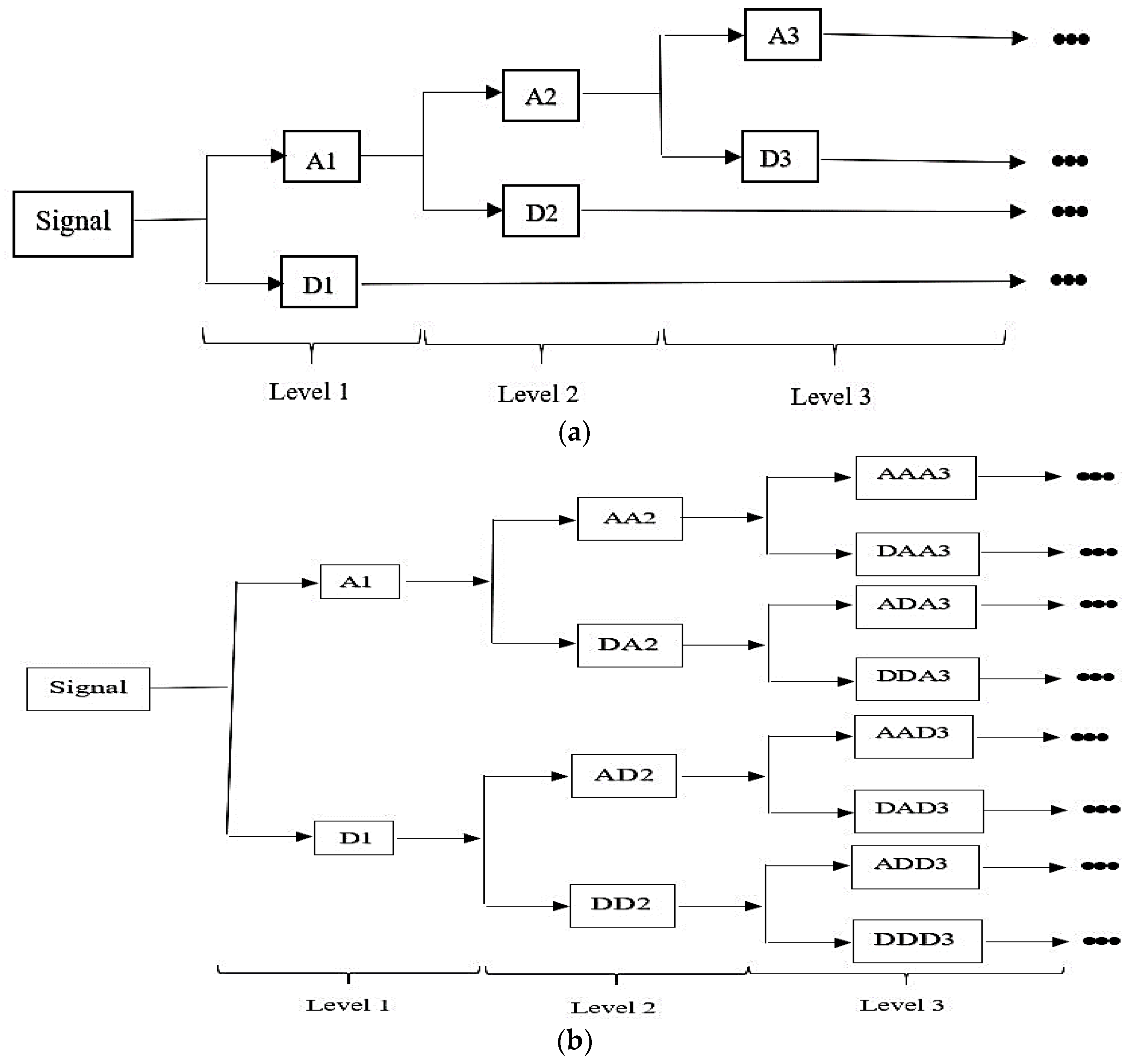
One of the prominent signal processing tools to examine steady state and non-stationary signals is the wavelet transform. Although the wavelet transform possesses capabilities to analyze local discontinuities of the signal, it also has some disadvantages, e.g., batch processing steps, non-uniform frequency sub-bands, less flexibility and a propensity to detection failures during noisy conditions. To overcome the mentioned issues, the wavelet packet transform (WPT) has been proposed in [36]. The decomposition process of the orthogonal wavelet and WPT is shown in Figure 4.

As can be observed in the orthogonal wavelet decomposition process, a signal is divided into two frequency bands, namely approximation coefficients (low frequency which is shown with capital A) and detail coefficients (higher frequency which is shown with capital D). The low frequency is utilized for further decomposition. Hence, the orthogonal wavelet gives a left recursive binary tree structure. However, because only the low frequency band is extracted, some properties of the high frequency band that have significant values in finding the local discontinuities of the signal are disregarded. This problem is solved by the WPT structure. As can be seen, both approximation coefficients and detail coefficients are split into two sub-bands and this process continues for further decomposition. Therefore, WPT gives a balanced binary tree structure and can provide a more accurate frequency resolution than orthogonal wavelet analysis.

Mathematically, the wavelet packet transform, which is a time-frequency function, can be written in the following form [37]:

$$W_{p,k}^i\left(t\right)=2^{\frac{p}{2}}{W}^i\left(2^{p}t-k\right)$$

(6)

where the scale and translation parameters are given by $p$ and $k$, respectively and $i=0,1,\dots$ is the index of the oscillation operation. The first two wavelet packet functions with $p=k=0$ are as follows:

$$\begin{gathered} W_{0,0}^0\left(t\right)=W^0\left(t\right)=\phi \left(t\right) \\ {W}_{0,0}^1\left(t\right)=W^1\left(t\right)=\psi \left(t\right) \end{gathered}$$

(7)

where $\phi \left(t\right)$ and $\psi \left(t\right)$ are called the scaling function and mother wavelet function, respectively. The other wavelet packet functions are expressed by the following equations:

$$\begin{gathered} W^{2i}\left(t\right)={\displaystyle \sum }_{k}h\left(k\right)W_{1,k}^i\left(t\right) \\ {W}^{2i+1}\left(t\right)={\displaystyle \sum }_{k}g\left(k\right)W_{1,k}^i\left(t\right) \end{gathered}$$

(8)

where $h\left(k\right)$ and $g\left(k\right)$ are low-pass filter and high-pass filter, respectively, and are shown as follows:

$$\begin{gathered} h\left(k\right)=\frac{1}{\sqrt{2}\langle \phi \left(t\right),\phi \left(2t-k\right)\rangle } \\ g\left(k\right)=1/\sqrt{2}\langle \psi \left(t\right),\psi \left(2t-k\right)\rangle \end{gathered}$$

(9)

The mentioned filters are orthogonal $g\left(k\right)={\left(-1\right)}^{k}h\left(1-k\right)$. Thus, from Equations (6) and (8), the following equations can be derived:

$$\begin{gathered} W^{2i}\left(t\right)=\sqrt{2}{\displaystyle \sum }_{k}h\left(k\right)W^i\left(2t-k\right) \\ {W}^{2i+1}\left(t\right)=\sqrt{2}{\displaystyle \sum }_{k}g\left(k\right)W^i\left(2t-k\right) \end{gathered}$$

(10)

Therefore, the wavelet packet coefficients $Y_{p,k}^i$ are computed by the inner product of the signal with each wavelet packet function as the following form:

$$Y_{p,k}^i=\langle x,W_{p,k}^i\rangle ={{\displaystyle \int }}_{-\infty }^{+\infty }x\left(t\right)W_{p,k}^i\left(t\right)dt$$

(11)

3.2. Feature Extraction Based on Shannon Entropy and Logarithmic Energy Entropy

A few approaches were studied for evaluating entropy of the random sequence $\left\{y_t\right\}$. The primary step in these approaches was to represent the data for relevant mapping of the continuous phase-space through the partition. The partitioning of a relevant sequence into disjoint sets was usually performed based on the uniform division of the block sizes. The estimation of entropy for the subsequent partitions was performed for the different block sizes correspondingly [38,39].

A common measure which can be utilized to find irregular patterns of the islanding and non-islanding signals is the information entropy. It would change due to different performances of signal frequency components for various conditions, whereby some of them may be removed and some may be raised. The measures of Shannon entropy and logarithmic energy entropy are calculated through the extracted WPT coefficients. The Shannon entropy is computed for each frequency band $i$ and $p$ level by the following Equation (12):

$$Entrop{y}_{p,i}=-{\displaystyle \sum }_{n=1}^N{\left|Y_{p,k}^i\left(n\right)\right|}^{2}log{\left|Y_{p,k}^i\left(n\right)\right|}^2$$

(12)

where n is the number of sampling point, whilst $Y_{p,k}^i$ is the extracted wavelet packet coefficients at the ith frequency band on the pth level, $i=2^p-1$.

The logarithmic energy entropy is computed as follows:

$$Energ{y}_{p,i}={\displaystyle \sum }_{n=1}^{N}log{[(Y_{p,k}^i\left(n\right))]}^2$$

(13)

where n is the number of sampling point, whilst $Y_{p,k}^i$ is the extracted wavelet packet coefficients at the i-th frequency band on the p-th level, $i=2^p-1$.

A feature database is generated by the aforementioned entropies, but before the obtained feature vectors are fed into classifiers as input vectors, they must be normalized. The normalized Shannon entropy (NSE) and logarithmic Energy Entropy (NLEE) are computed using the following expressions:

$$\begin{gathered} Entrop{y}_p=\frac{Entrop{y}_{p,i}}{{{\displaystyle \sum }}_{p=0}^{2^p-1}Entrop{y}_{p,i}} \\ Energ{y}_p=\frac{Energ{y}_{p,i}}{{{\displaystyle \sum }}_{p=0}^{2^p-1}Energ{y}_{p,i}} \end{gathered}$$

(14)

3.3. Probabilistic Neural Network

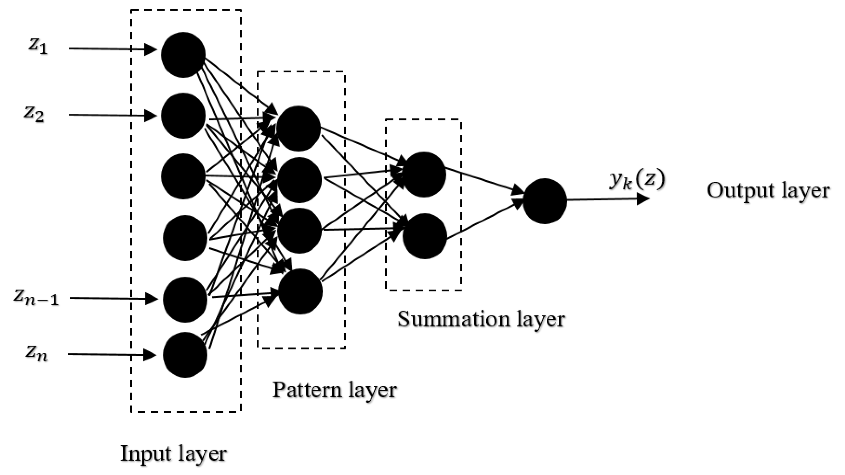
The probabilistic neural network is one of the most powerful neural networks utilized for pattern recognition and classification in power systems because of some advantages such as quick training process, easy addition and removal of training samples without retraining, and no local minima [40]. PNN is fundamentally formed based on a Bayesian Decision criterion and owing to its high training speed and good accuracy, it is suitable for signal classification systems and real time fault detection [41]. Figure 5 illustrates a PNN structure that consists of four layers, namely the input layer, the pattern layer, the summation layer, and the output layer [42].

The first layer is the input layer that distributes the input vector to each neuron in the pattern layer which consists of nonlinear radial basis activation functions. In the second layer, the number of neurons is the amount of samples in the training set. The neurons perform a weighted sum of the receiving signal from the input layer which is then applied to a nonlinear radial basis activation function for the neuron output. The nonlinear activation function equation is considered as follows [43]:

$$\phi (\Vert z_{wi}-1{\Vert }_2)=e^{\frac{\Vert z_{wi}-1{\Vert }^2}{{\sigma }_i^2}}$$

(15)

where $z_{wi }$ is the weight of the input of $z_i$ to the neuron and $\sigma$ is the smoothing factor. Pattern layer is utilized to compute the matching degree between the input feature vector and the classes of the training set, which determines the probability that the vector belongs to a class. The output of the pattern layer is transmitted to a single summation layer neuron that can be computed as follows:

$$R_k\left(z\right)={\displaystyle \sum }_{i=1}^k\phi \left(\Vert z_{wi}-1{\Vert }_2\right)={\displaystyle \sum }_{i=1}^k{e}^{\frac{\Vert z_{wi}-1{\Vert }^2}{{\sigma }_i^2}}, k=2,3,4,\dots$$

(16)

where $k$ is the total number of classes.

The output of summation units is transmitted to each neuron of the output layer. Finally, neurons in the output layer make decisions on the class for each input pattern layer $z$ through the Bayesian strategy. Thus, the output is formulated as follows:

$$y_k\left(z\right)=\arg \left(max\left\{R_k\left(z\right)\right\}\right)$$

(17)

The main factor which must be selected for training is the smoothing factor. A reasonable range would be from 0.001 to 0.009 and from 0.01 to 0.09. Another important factor in the PNN are the weights that are adjusted based on [30].

3.4. Proposed Islanding Detection

In order to examine the transient events which are short-term and non-stationary signals in a power grid, WPT can be utilized as an effective tool. It can be utilized to recognize and classify different conditions and events. Islanding events and grid faults are non-stationary waveforms. WPT of transient signals of the mentioned events is used to derive features vector needed for classification. The specific signature of transient waveforms is determined by feature derivation which can be utilized to differentiate islanding and grid faults condition. In this study, the specific signatures of the PCC voltage signals of islanding events and grid faults are determined by feature extraction which will be used in distinguishing between islanding and grid faults cases. The steps in generating the feature vectors needed for classification are as follows:

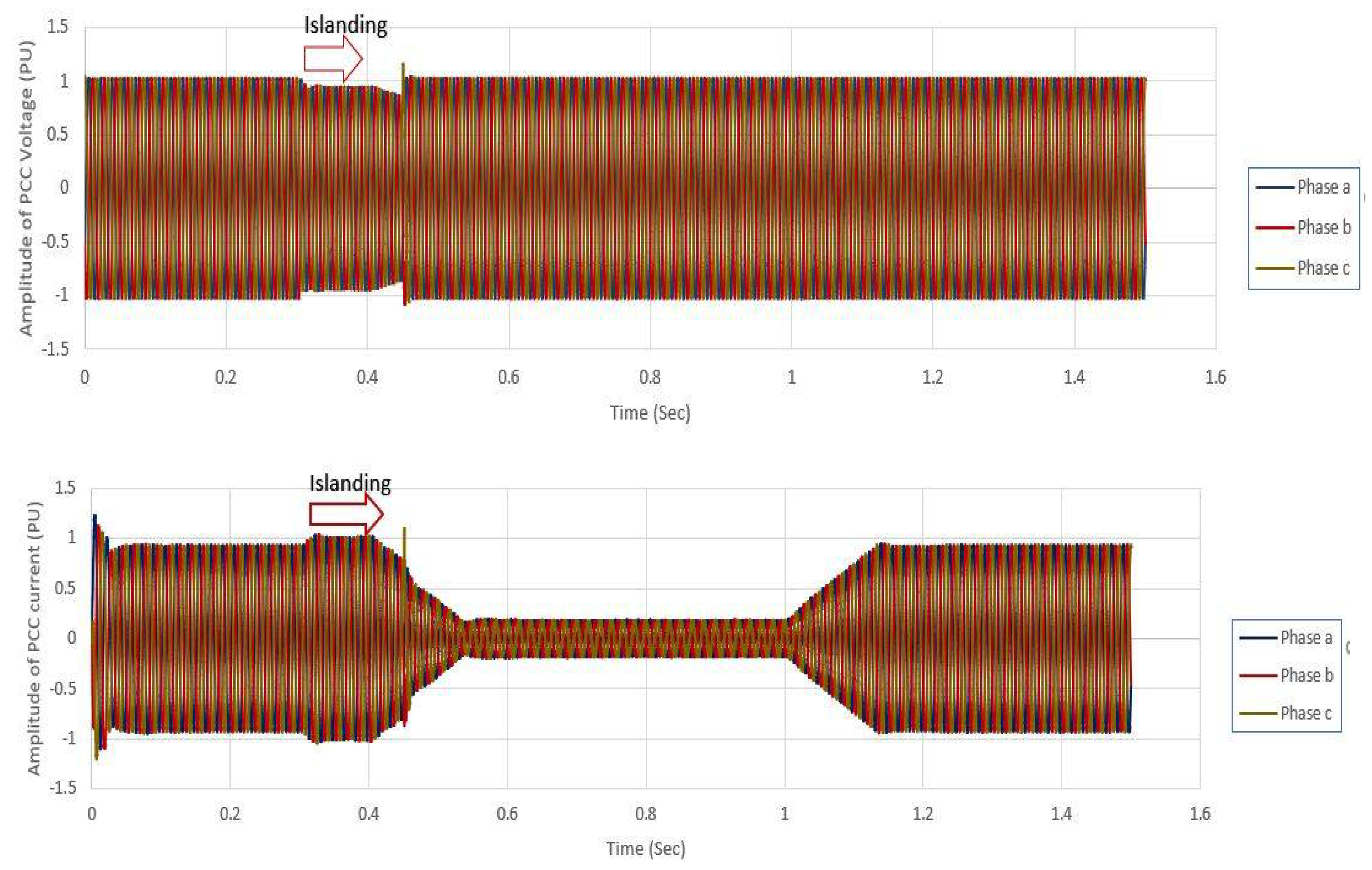
• Step 1. The PCC voltage signals of islanding cases and grid faults cases which are mentioned in Table 1 are obtained by simulation in the Matlab/Simulink environment. As an example, Figure 6 illustrates the PCC voltage and current signals once the local loads match the local generation in the aforementioned islanding case. An islanding scenario is created once the circuit breaker (SW₁) is opened at t = 0.3 s (5940th point) and closed after 0.15 s e.g., t = 0.45 s (the 8910th point). The sampling frequency of signal is 19.8 kHz whilst the sampling number for each period is 330 points. In addition, the time of simulation is 1.5 s and the total sampling number is 29,700 points.
• Step 2. The PCC voltage signals of islanding cases and grid faults cases are decomposed into different frequency bands by WPT. The performance of the proposed islanding detection is related to the selection of a suitable mother wavelet. The mother wavelet has an important role in the analysis. One of the appropriate wavelet families which has been used to examine the transient events is Daubechies’ wavelet families [44,45]. In this work, some-widely-used mother wavelets from Daubechies family, including db1, db4, db7, and db20, are analyzed. In order to derive a more predominant group of feature vectors, the decomposition level of wavelet packet for each signal is up to 6 levels.

  Table 2. Frequency bands of each level.

  WPT Level	Frequency Bands (Hz)
  1	0–4950, 4950–9900
  2	0–2475, 2475–4950, 4950–7425, 7425–9900
  3	0–1237.5, 1237.5–2475, 2475–3712.5, 3712.5–4950, 4950–6187.5, 6187.5–7425, 7425–8662.5, 8662.5–9900
  4	0–618.75, 618.75–1237.5, 1237.5–1856.25, 1856.25–2475, 2475–3093.75, 3093.75–3712.5, 3712.5–4331.25, 4331.25–4950, 4950–5568.75, 5568.75–6187.5, 6187.5–6806.25, 6806.25–7425, 7425–8043.75, 8043.75–8662.5, 866.5–9281.25, 9281.25–9900
  5	0–309.375, 309.375–618.75, 618.75–928.125, 928.125–1237.5, 1237.5–1546.875, 1546.875–1856.25, 1856.25–2165.625, 2165.625–2475, 2475–2784.375, 2784.375–3093.75, 3093.75–3403.125, 3403.125–3712.5, 3712.5–4021.875, 4021875–4331.25, 4331.25–4640.625, 4640.625–4950, 4950–5259.375, 5259.375–5568.75, 5568.75–5878.125, 5878.125–6187.5, 6187.5–6496.875, 6496.875–6806.25, 6806.25–7115.625, 7115.625–7425, 7425–7734.375, 7734.375–8043.75, 8043.75–8353.125, 8353.125–8662.5, 8662.5–8971.875, 8971.875–9281.25, 9281.25–9590.625, 9590.625–9900
  6	0–154.6875, 154.68.75–309.375, 309.375–464.0625, 464.0625–618.75, 618.75–773.4375, 773.4375–928.125, 928.125–1082.8125, 1082.8125–1237.5, 1237.5–1392.1875, 1392.1875–1546.875, 1546.875–1701.5625, 1701.5625–1856.25, 1825.25–2010.9375, 2010.9375–2165.625, 2165.625–2320.3125, 2320.3125–2475, 2475–2629.6875, 2629.6875–2784.375, 2784.375–2939.0625, 2939.0625–3093.75, 3093.75–3248.4375, 3248.4375–3403.125, 3403.125–3557.8125, 3557.8125–3712.5, 3712.5–3867.1875, 3867.1875–4021.875, 4021.875–4176.5625, 4176.5625–4331.25, 4331.25–4485.9375, 4485.9375–4640.625, 4640.625– 4795.312, 4795.312–4950, 4950–5104.6875, 5104.6875–5259.375, 5259.375–5414.0625, 5414.0625–5568.75, 5568.75–5723.4375, 5723.4375–5878.125–6032.8125, 6032.8125–6187.5, 6187.5–6342.1875, 6342.1875–6496.875, 6496.875–6651.5625, 6651.5625–6806.25, 6806.25–6960.9375, 6960.9375–7115.625, 7115.625–7270.3125, 7270.3125–7425, 7425–7579.6875, 7579.6875–7734.375, 7734.375–7889.0625, 7889.0625–8043.75, 8043.75–8198.4375, 8198.4375–8353.125, 8353.125–8507.8125, 8507.8125–8662.5, 8662.5–8817.1875, 8817.1875–8971.875, 8971.875–9126.5625, 9126.5625–9281.25, 9281.25–9435.9375, 9435.9375–9590.625, 9590.625–9745.3125, 9745.3125–9900

  summarizes the frequency bands of each level.
• Step 3. The calculation of NSE and NLEE of the PCC voltage. According to IEEE Std. 1547, distributed generation systems such as photovoltaic (PV) inverter output currents should have low distortion levels. This means the entire current distortion should not exceed 5% of the fundamental current [46]. The main harmonics of the inverter output current are of 3rd, 5th, 7th, and 9th orders and the frequency range of high-frequency components of the PCC voltage signal commonly falls in a range of 160–1900 Hz. Thus, this range of frequency can be found in band 2 (154.68.75–309.375), band 3 (309.375–464.0625), band 4 (464.0625–618.75), band 5 (618.75–773.4375), band 6 (773.4375–928.125), band 7(928.125–1082.8125), band 8 (1082.8125–1237.5), and band 13 (1825.25–2010.9375). Hence, in order to calculate NSE and NLEE of the PCC voltage, the mentioned frequency bands are utilized as the most appropriate decomposition frequency bands.
• Step 4. The obtained features (NSE and NLEE) are fed into PNN classifier to distinguish between islanding events and grid faults.

In order to obtain the best performance of the proposed islanding detection algorithm in terms of accuracy, speed, cost, and simplicity, the method is analyzed for different aspects as follows:

(a)

Selection of suitable feature applied to PNN classifier.

• The PNN classifier decides based on NSE. The islanding detection method is designated by (NSE).
• The PNN classifier decides based on NLEE. The islanding detection method is designated by (NLEE).
• The PNN classifier decides based on NSE and NLEE. The islanding detection method is designated by (NLEE and NSE).

(b)

The aforementioned islanding detection techniques were investigated with four different mother wavelets from the Daubechies family, including db1, db4, db7, and db20.

(c)

The aforementioned islanding detection techniques were estimated at level 1–6.

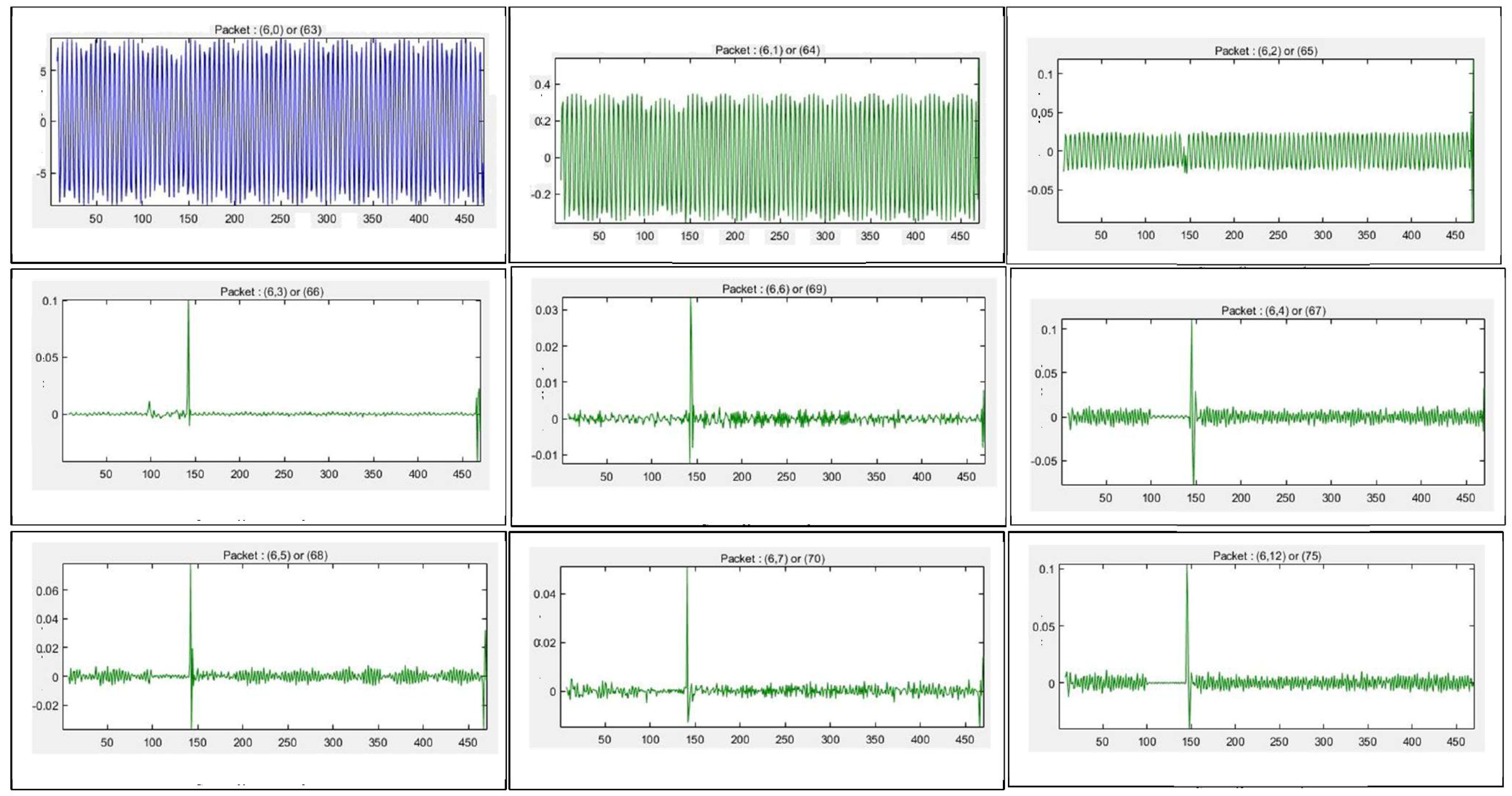
Figure 7 shows the wavelet packet coefficients (WPCs) of the mentioned frequency bands in step 3 for the PCC voltage signal once the local loads match with local generation in the islanding event mentioned in Step 1. It can be seen that the magnitude of the WPC during islanding conditions varies, especially in the mentioned frequency bands in step 3 in comparison with normal conditions. Nodes (6,1), (6,2), (6,3), (6,4), (6,5), (6,6), (6,7), and (6,12) are utilized as the most appropriate decomposition frequency bands in order to obtain feature vectors (NSE and NLEE). The NLEE and NSE values of these nodes will be computed for the mentioned cases in Table 1. The NLEE values of Nodes (6,1), (6,2), (6,3), (6,4), (6,5), (6,6), (6,7), and (6,12) are $Energ{y}_1, Energ{y}_2, Energ{y}_3, Energ{y}_4, Energ{y}_5, Energ{y}_6, Energ{y}_7, \mathrm{and} Energ{y}_8$ respectively and their NSE values are $Entrop{y}_1, Entrop{y}_2, Entrop{y}_3, Entrop{y}_4, Entrop{y}_5, Entrop{y}_6, Entrop{y}_7, \mathrm{and} Entrop{y}_8$, respectively. These values are utilized as a feature vector in this work.

As seen in Figure 8, the working process of the proposed algorithm is summarized as follows: First, one cycle of the sampled three phase PCC voltage signals is selected to compute the wavelet packet nodes matrix. The sampling frequency of the three phase PCC voltage is 19.8 kHz and each cycle has 330 samples. Second, the PCC voltage is decomposed into 64 different bands (Level 6) by multiresolution wavelet packets with (db1, db4, db7, and db20) and two feature values i.e., NSE and NLEE for each frequency band will be computed. The generated feature vector is fed to the classification phase, i.e., the PNN classifier. Finally, in order to determine whether islanding occurs or not, the command block will be executed so that if islanding cases are detected, the proposed islanding scheme transfers a “trip signal is set to 1” command, whilst for non-islanding cases (grid faults) a “trip signal is set to 0” command is set. The proposed islanding detection scheme can also be executed on a DSP/FPGA board to manage the protection relay behavior during islanding cases and non-islanding cases. Figure 8 illustrates the block diagram of the proposed islanding detection method based on the combination of WPT and PNN.

4. Results and Discussion

4.1. Simulation Results

In order to evaluate the proposed islanding detection scheme, a 250-kW grid-connected photovoltaic array was simulated in the Matlab environment as shown in Figure 1. The simulated system includes several parts mentioned in Section 2.1. The events in Table 1 are simulated off-line to derive important features of the system behavior. The definition of these events is based on two main sources as follows: firstly, the operational requirements in the IEEE1547 standards and secondly, the test practices that are recommended by most of the manufacturers of islanding relays. The events can be considered divided into three main categories: normal condition, islanding condition and grid faults. In order to form the islanding cases, circuit breaker SW₁ is opened at t = 0.3 s and closed after 0.15 s. The whole simulation time is 1.5 s. As mentioned in Table 1, in order to create islanding scenarios, connected loads in the power grid need to be considered. Hence, three scenarios are taken into account in this study. The first scenario is created when the local loads match the local generation.

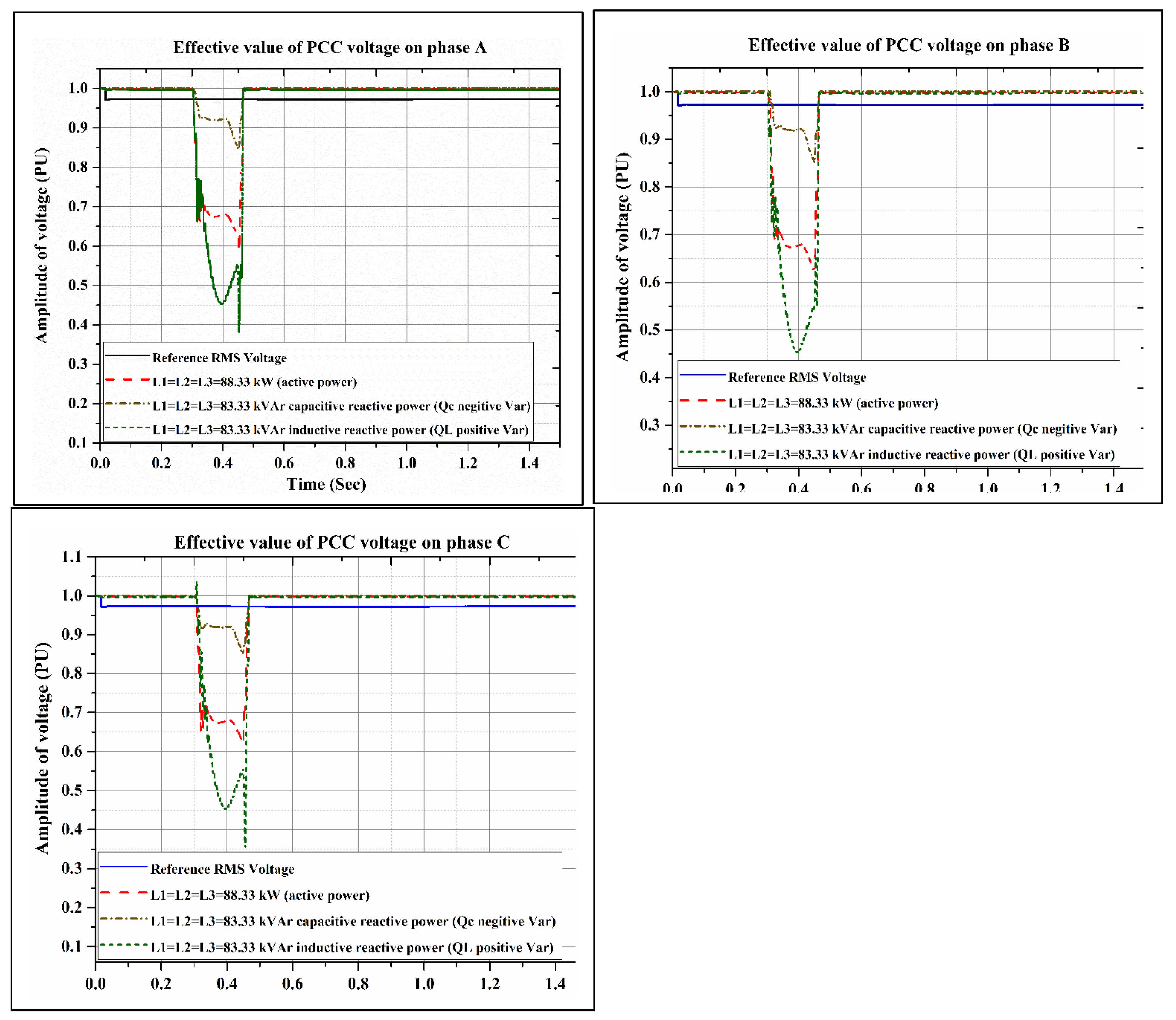
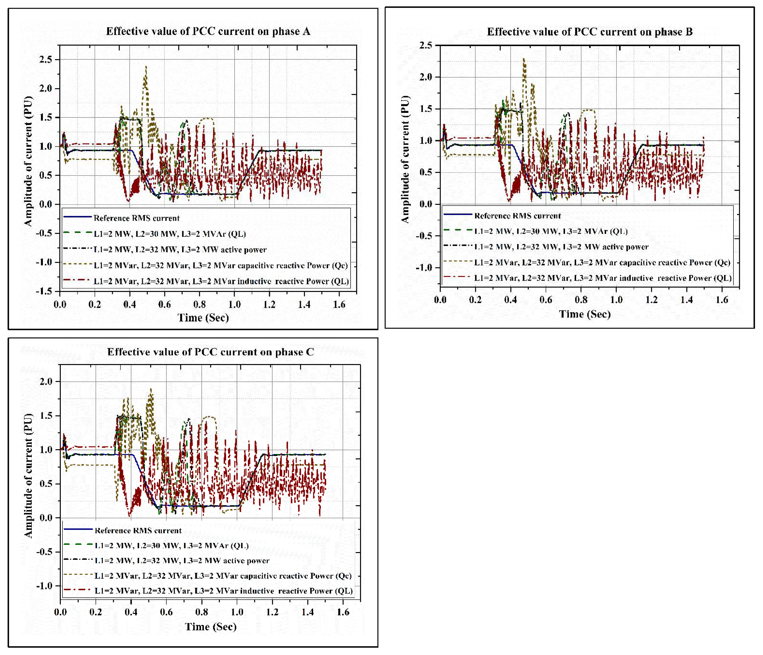
The effective value of the grid voltage and current measured at the PCC, and also the variation of frequency of the PCC voltage for different configurations of the connected feeder loads are shown in Figure 9, Figure 10 and Figure 11.

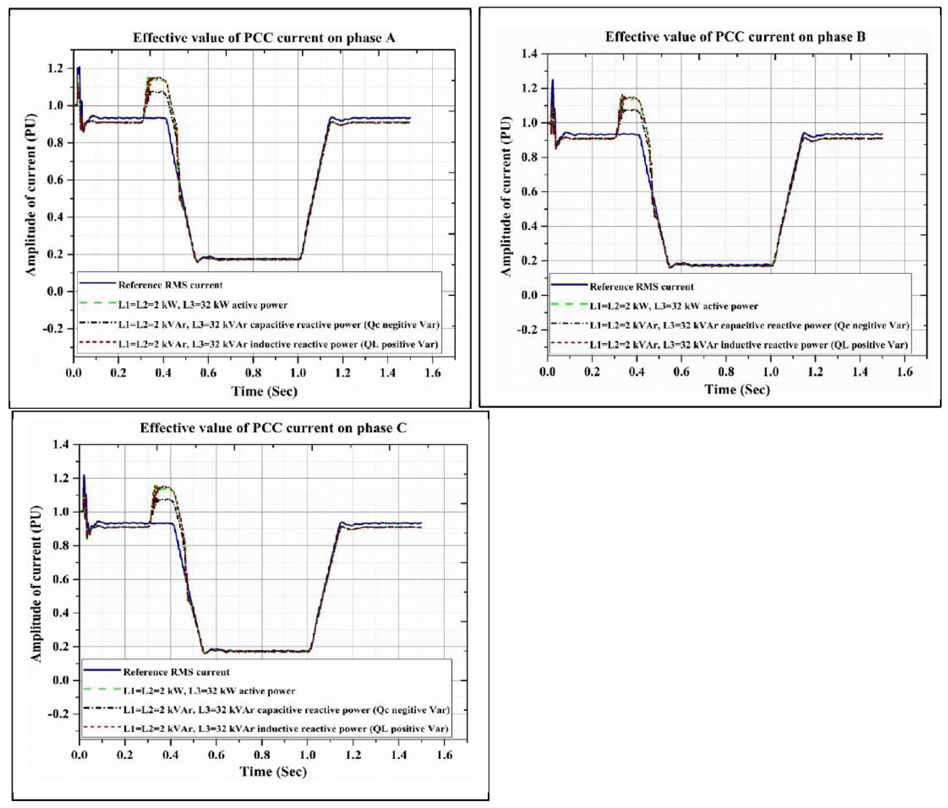
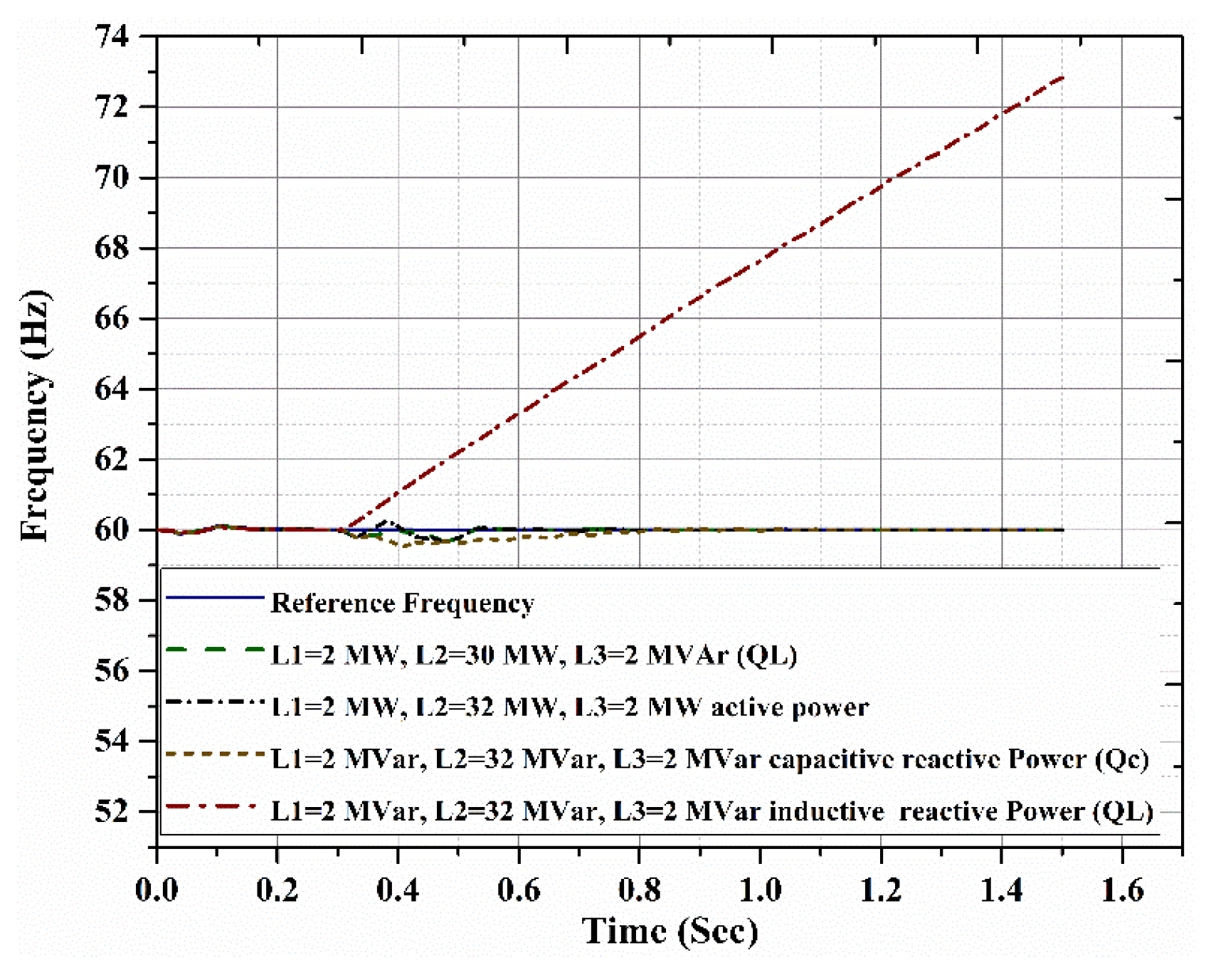
According to the IEEE Std. 1547, the permissible variation of frequency range is between 59.3 Hz and 60.5 Hz. The permissible range of variation for the voltage is between 0.88 (pu) and 1.2 (pu). If variations of PCC voltage and frequency are within the permissible ranges, the variations of normal relays are interoperated as normal conditions, otherwise, the condition is recognized as an islanding event. Hence, as can be observed in Figure 9 and Figure 11, the variations of the PCC voltage and frequency for capacitive reactive power loads are within the permissible ranges. Thus, this case is not detected as islanding by the relays. Nonetheless, for other loads such as active power loads and inductive reactive power loads, the variations of the PCC voltage exceeded the permissible range of the voltage and are detected as islanding by normal protection relays, whilst their variations of frequency are within the permissible range. The second islanding scenario is created when local loads are smaller than the local generation. The variations of PCC voltage and current and also frequency is shown in Figure 12, Figure 13 and Figure 14.

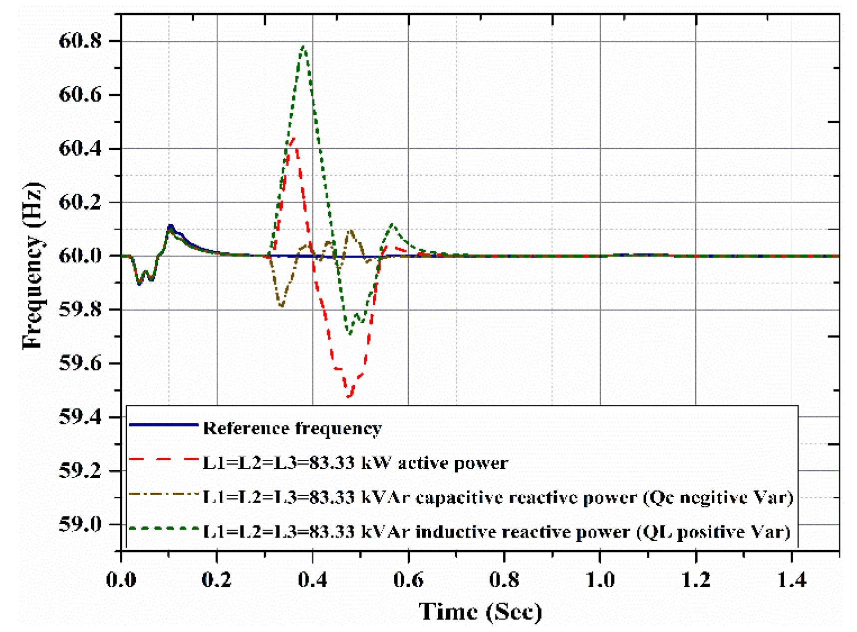
As shown in Figure 12, the amplitude variations of the PCC voltage for active power loads and capacitive reactive power loads are within the permissible range. However, the value exceeds the permissible range for inductive reactive power loads. Figure 14 illustrates the variations of the frequency of the PCC voltage for all local loads which remains in the acceptable range after islanding happened. Hence, the islanding detection method based on normal protection relays failed to detect the islanding case in scenario 2. The third islanding scenario is created once local loads are greater than local generation. Figure 15, Figure 16 and Figure 17 illustrate the variations of effective value of PCC voltage and current, and the variation of frequency of PCC voltage, respectively.

As can be seen, when islanding occurred, the amplitude of the PCC voltage exceeds the permissible range. The variations of frequency for all loads are quite close except for the inductive reactive power loads. Hence, it can be said that the worst-case studies of islanding are once the amplitude of the PCC voltage and its variation of frequency are within permissible range. The number of islanding according to the aforementioned scenarios is 120. The performance of the proposed method in detecting these cases will be discussed in the next section.

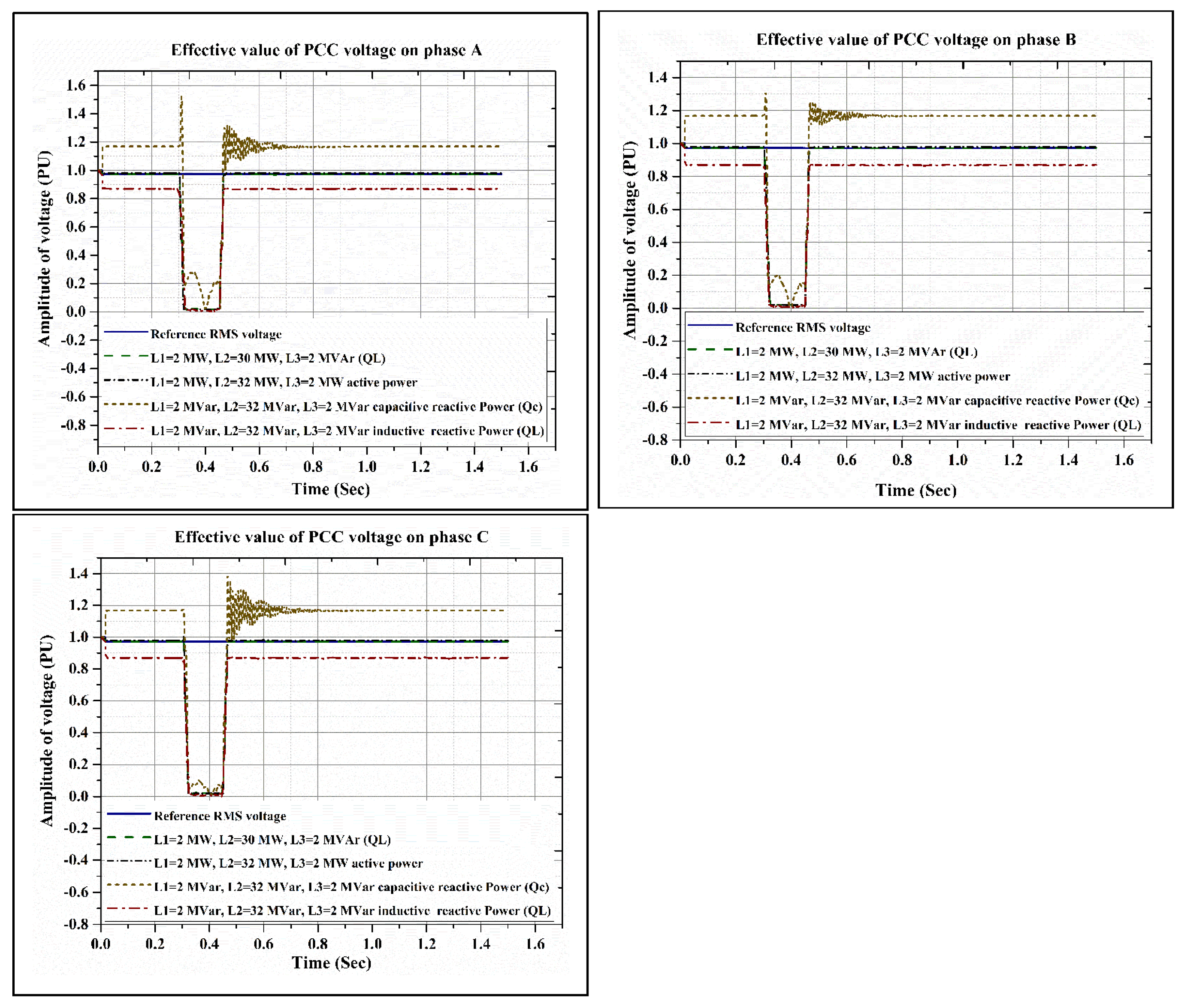
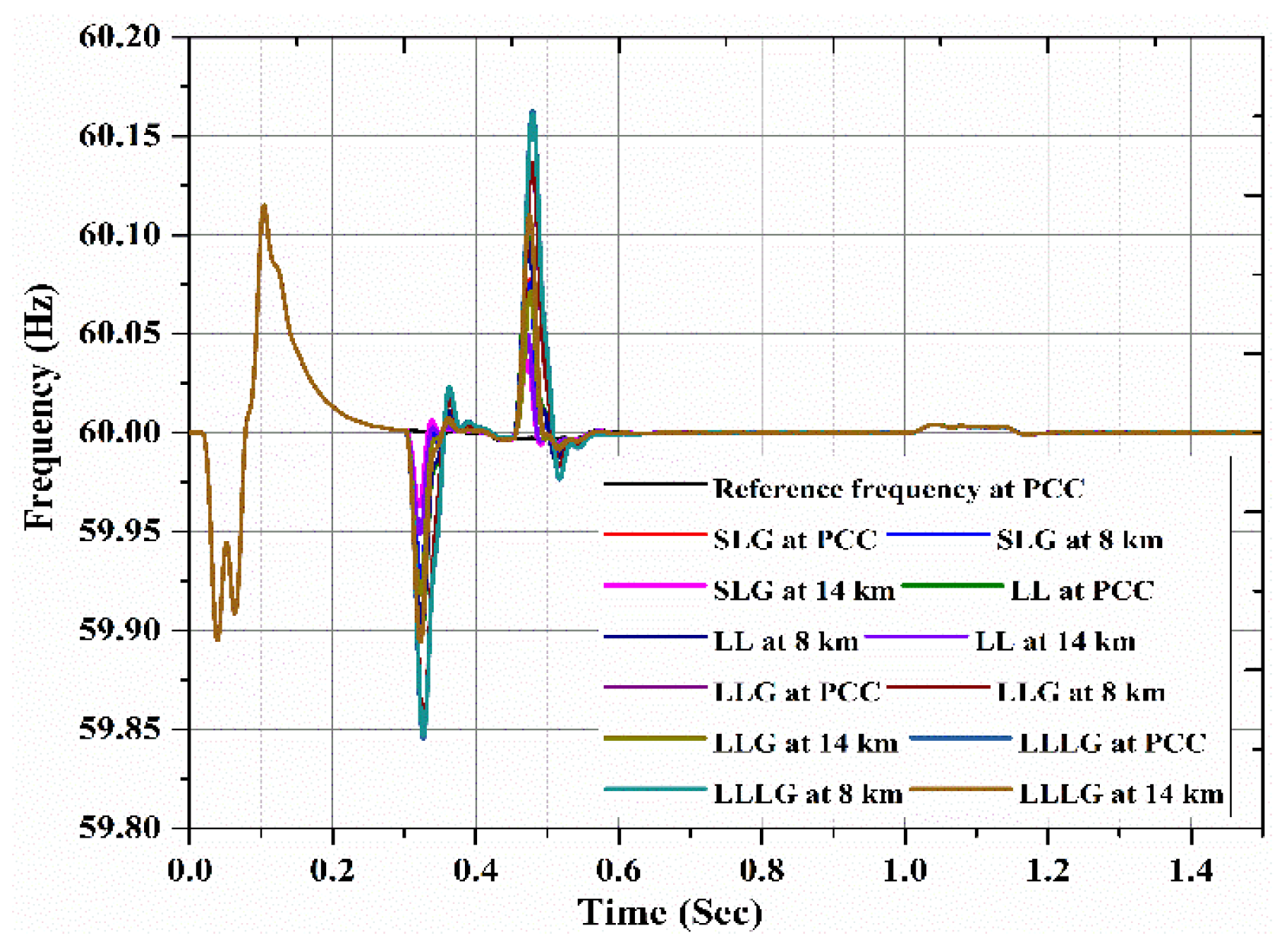
Different grid faults which may occur in the utility grid are also taken into account. The different fault conditions include: single phase to ground (SL-G), double phase to ground and line to line fault (LL, LL-G), and three phase fault (LLL-G) whose resistance (0–200 ohms) are applied in t = 0.3 s and cleared after 0.15 s. The locations of the grid faults are near the PCC, and at distances of 8 km, and 14 km as shown in Figure 1. Once the faults occurred, the protection relay should timely detect abnormal voltage variations and then disconnect the distributed generation from the main utility grid. Thus, these cases should not be detected as islanding before the relay operates.

Table 3. Voltage relay responses.

Voltage Range (% of Base Voltage)	Clearing Time (s)
V < 50 50% < V < 88 110 < V < 120 V > 120%	0.16 2 1 0.16

illustrates the voltage relay responses for abnormal conditions based on the IEEE Std. 1547 [47]. The effective value of the PCC voltage and the variations of frequency for different grid faults with 200 ohms resistance are shown in Figure 18 and Figure 19.

As can be observed, the variations of the amplitude of PCC voltage and frequency are insignificant once the short circuit faults occurred. The detection of islanding condition from non-islanding cases (grid faults) is a problem. The performance of the proposed method for identification of islanding and grid faults will be discussed in the next section.

4.2. Performance of the Proposed Islanding Detection Algorithm

In order to evaluate the efficiency of the proposed features as input data for PNN classifier, a conventional validation is done. The number of islanding and grid faults events simulated are 220 cases. Among them, a random extraction of 10%, 20%, 30%, and 40% cases out of the input databases are used as testing subsets and the rest of the patterns e.g., 90%, 80%, 70%, and 60% of data are used as training sets. In order to train PNN classifier, several spread factors in the hidden layer activation is selected experimentally from the interval [0.001–0.009] and [0.01–0.09] and only the best results are presented. In order to evaluate the performance of the proposed islanding detection method, several parameters such as sensitivity (R1), specificity (R2), and overall accuracy (R3) are calculated as follows [48]:

$$R1=sensitivity=\frac{TP}{\left(TP+FN\right)}$$

(18)

$$R2=specificity=\frac{TN}{\left(TN+FP\right)}$$

(19)

$$R3=overall accuracy=\frac{\left(TP+TN\right)}{\left(TP+TN+FP+FN\right)}$$

(20)

where, TP is true positive; the total number of islanding detected correctly. TN is true negative; the number of grid faults detected correctly. FN is false negative; the total number of islanding case detected as grid faults. FP is false positive; the number of grid faults detected as islanding. The performance of the islanding detection algorithm is assessed in different aspects as follows.

4.2.1. Evaluation of the Proposed Method from Input Features Point of View

In order to obtain optimal islanding detection method, the proposed technique is evaluated in terms of input features to determine which features are more effective for islanding detection. As can be observed in

Table 4. PNN classification results at level 6 of wavelet packet decomposition using “db1”.

Features	Spread Factor	Data Partitions (%)
		60/40			70/30			80/20			90/10
		R1	R2	R3	R1	R2	R3	R1	R2	R3	R1	R2	R3
NSE	0.008	77.63	73.37	75.20	83.39	79.13	81.25	85.37	81.69	83.33	86.10	83.97	85.01
	0.02	78.35	74.11	76.04	84.63	79.51	81.86	86.89	82.86	84.61	87.30	83.63	85.42
	0.03	81.76	75.09	78.03	85.14	81.42	82.97	86.65	83.26	84.80	88.15	84.80	86.39
	0.04	82.92	74.02	78.53	85.25	80.57	82.33	86.31	83.83	85.14	88.73	84.52	86.41
NLEE	0.006	79.87	77.51	78.02	83.47	79.60	81.19	86.95	82.59	84.11	86.87	83.51	85.13
	0.01	81.16	77.89	79.55	84.10	80.93	82.38	88.16	83.73	85.91	87.13	84.60	85.52
	0.02	82.29	78.68	80.71	84.24	82.14	83.14	87.65	84.31	85.74	88.35	85.32	87.62
	0.03	83.30	77.15	80.43	85.25	82.34	83.45	89.38	86.14	88.42	89.89	86.79	88.12
NLEE+NSE	0.005	82.43	80.33	80.60	85.48	83.12	83.52	87.88	85.66	86.43	91.11	88.58	90.19
	0.007	83.66	81.22	81.77	86.69	83.19	84.60	89.40	86.41	87.13	92.40	89.28	91.62
	0.01	84.31	80.68	82.13	87.72	82.51	84.93	90.37	86.75	89.08	93.53	90.23	91.81
	0.08	85.79	81.53	82.81	86.20	84.24	85.47	91.22	88.73	89.54	93.69	89.73	91.53

,

Table 5. PNN classification results at level 6 of wavelet packet decomposition using “db4”.

Features	Spread Factor	Data Partitions
		60/40			70/30			80/20			90/10
		R1	R2	R3	R1	R2	R3	R1	R2	R3	R1	R2	R3
NSE	0.005	81.37	79.41	80.33	84.90	80.56	82.29	86.36	82.31	84.86	88.24	84.33	86.37
	0.006	81.53	80.28	80.67	86.02	81.22	83.10	88.01	83.10	85.72	90.71	85.21	87.55
	0.03	84.78	80.71	82.10	87.37	81.59	84.53	89.13	83.98	86.21	91.34	86.43	88.52
	0.08	85.48	81.65	83.57	87.51	82.37	85.02	89.26	84.05	86.59	92.33	87.11	89.65
NLEE	0.004	83.52	81.22	82.34	87.16	82.11	84.40	89.43	84.98	87.28	92.69	87.08	89.36
	0.007	84.30	81.52	82.61	88.28	82.89	85.44	90.82	84.46	87.57	93.63	87.66	90.71
	0.01	86.15	82.18	84.07	88.51	83.41	85.82	92.48	86.34	89.48	94.56	88.37	91.31
	0.08	86.81	83.06	84.77	88.12	83.86	86.04	92.81	86.86	89.90	94.14	88.20	91.15
NLEE+NSE	0.006	88.23	84.03	86.08	90.46	86.44	88.69	92.61	88.72	90.74	94.24	91.63	92.85
	0.008	90.58	86.73	88.42	92.61	87.10	89.13	93.07	89.60	91.38	95.16	92.14	93.49
	0.04	91.92	86.26	89.16	93.19	87.62	90.56	95.83	89.33	92.85	96.87	92.52	94.38
	0.09	90.38	86.94	88.63	93.33	88.40	90.71	95.25	90.61	93.01	96.39	92.31	94.18

,

Table 6. PNN classification results at level 6 of wavelet packet decomposition using “db7”.

Features	Spread Factor	Data Partitions
		60/40			70/30			80/20			90/10
		R1	R2	R3	R1	R2	R3	R1	R2	R3	R1	R2	R3
NSE	0.006	82.63	80.79	81.19	86.50	84.14	85.39	88.35	87.36	87.34	91.77	90.60	91.08
	0.01	84.52	81.26	82.51	88.76	83.86	86.23	90.47	90.51	90.33	93.34	91.25	92.37
	0.03	84.56	81.89	83.16	87.73	84.31	86.08	90.26	90.97	90.41	93.48	90.82	92.10
	0.08	85.17	82.41	83.35	88.39	84.53	86.62	92.43	91.54	91.21	94.73	91.77	93.11
NLEE	0.005	85.47	83.37	84.08	88.18	87.66	87.58	91.49	89.48	90.17	93.11	90.41	91.42
	0.02	85.03	84.51	84.22	89.71	88.19	88.61	91.08	90.11	90.44	93.97	91.69	92.17
	0.04	87.63	85.31	86.24	89.52	88.10	88.29	93.53	90.61	92.05	95.29	93.73	94.35
	0.09	86.10	84.83	85.16	91.99	89.63	90.37	93.86	91.36	92.51	95.60	93.94	94.54
NLEE+NSE	0.009	88.71	86.25	87.39	91.13	90.14	90.41	93.57	92.10	92.63	95.83	95.36	95.42
	0.01	90.47	88.13	89.17	93.57	92.89	93.27	95.20	93.65	94.29	97.47	95.74	96.71
	0.03	91.11	88.51	89.29	94.30	93.23	93.60	95.79	93.84	94.48	97.40	95.73	96.53
	0.09	91.78	89.72	90.31	94.68	93.61	94.11	96.19	93.98	95.15	97.54	96.18	96.77

and

Table 7. PNN classification results at level 6 of wavelet packet decomposition using “db20”.

Features	Spread Factor	Data Partitions
		60/40			70/30			80/20			90/10
		R1	R2	R3	R1	R2	R3	R1	R2	R3	R1	R2	R3
NSE	0.007	86.10	85.38	85.45	87.89	85.57	86.72	91.45	89.85	90.21	93.68	93.25	93.31
	0.01	86.32	85.71	86.08	88.90	87.16	88.09	93.31	91.32	92.18	92.71	91.81	92.20
	0.04	86.14	84.62	85.22	90.55	87.31	88.68	93.18	91.67	92.30	94.22	93.59	93.39
	0.08	87.56	86.33	86.84	90.43	89.49	89.61	92.24	92.18	92.13	94.36	93.96	94.07
NLEE	0.009	86.19	86.22	91.11	90.31	89.81	90.13	93.27	93.51	93.28	95.33	94.65	94.86
	0.01	88.38	87.39	87.53	92.20	91.14	91.53	93.55	93.20	93.19	96.21	95.61	95.73
	0.03	87.94	87.27	87.42	92.79	91.31	92.11	93.71	94.44	94.12	95.48	95.26	95.22
	0.08	88.79	87.88	88.18	91.90	90.77	91.48	94.12	94.85	94.41	96.16	95.35	95.82
NLEE+NSE	0.008	92.66	92.11	92.42	95.20	95.28	95.37	97.87	97.00	97.50	98.14	98.66	98.36
	0.01	94.39	93.60	93.83	97.35	96.40	96.63	98.53	98.49	98.27	98.85	99.10	98.85
	0.02	95.45	93.84	94.37	97.48	96.32	96.82	98.60	97.03	97.77	99.56	99.37	99.56
	0.09	95.90	94.23	95.02	96.32	96.53	96.33	97.39	97.26	97.42	99.93	99.67	99.87

, the results are divided into three separate feature groups as input data for PNN classifier, namely NSE, NLEE, and NLEE+NSE, with four different mother wavelets from Daubechies family, including “db1”, “db4”, “db7”, and “db20” at level 6 in different spread factors. In order to train the PNN, several data partitions were executed as observed in tables. Form tables, it was found that the combination of NLEE and NSE features as input data to PNN classifier have better performance than other features. A predominant group of feature vectors which were provided by (NSE+NLEE) increased the classification accuracy. The highest classification accuracy was for (NSE+NLEE) at data partitions of 90/10. As can be seen from Table 4, the classification accuracy was computed for different data partitions based on the mentioned features. The increase in classification accuracy with data partitions change is obvious. The percentage of this accuracy is 12% for NSE, 11% for NLEE, and 13% for (NSE+NLEE). The best overall accuracy for NSE, NLEE and (NSE+NLEE) is 86.41, 88.12, and 91.53% at data partition (90/10). Hence, the best performance of the detection method in Table 4 was obtained for (NSE+NLEE) at data partition of 90/10 with spread factor of 0.04. From Table 5, the percentage of increase in classification accuracy is 8% for NSE, 10% for NLEE, and 11% for (NLEE+NSE). For Daubechies wavelet “db4”, the performance of NLEE+NSE is better than the others. The best performance from Table 5 was obtained for (NSE+NLEE) at data partition of 90/10 in spread factor of 0.08. In Table 6 and Table 7, the best performance went to (NSE+NLEE) at data partition of 90/10. For Daubechies wavelet “db7”, the best overall accuracy is 96.77% for (NSE+NLEE) at data partition of 90/10 and spread factor of 0.09, whilst the performance of NLEE is almost equal to that of NSE. The performance of (NSE+NLEE) in data partition 90/10 with spread factor 0.09 is better than other performance. As a conclusion, the proposed islanding method based on (NSE+NLEE) is preferred to other methods based on NSE and NLEE, as it is able to reduce the NDZ.

4.2.2. Evaluation of the Proposed Islanding Method in Terms of Mother Wavelet

The islanding and gird faults signals were filtered by wavelet packet filters with four different mother wavelets from Daubechies family, including “db1”, “db4”, “db7”, and “db20” at level 6. In order to select the optimal mother wavelet, the proposed islanding detection method was evaluated for mother wavelets separately in Table 4, Table 5, Table 6 and Table 7. As can be observed, the best performance of PNN classifier is obtained when (NSE+NLEE) is used as input data of PNN classifier for different mother wavelets namely “db1”, “db4”, “db7”, and “db20”.

However, in order to select the optimal mother wavelets, the performance of the PNN classifier need to be considered. As can be seen from Table 4, Table 5, Table 6 and Table 7, the lowest sensitivity (R1), specificity (R2), and overall accuracy (R3) were for Daubechies wavelet “db1”. For “db4” and “db7”, the performance of their PNN classifier is average. The maximum percentage of sensitivity (R1), specificity (R2), and overall accuracy (R3) were obtained for “db20”. Its overall accuracy is 99.87 at data partition 90/10 and it shows that the proposed feature and classification algorithm provides better classification in comparison to that of the other three types. In summary, the optimal detection method for grid tied PV system would be ((NSE+NLEE)-db20-6) which must be evaluated under noisy environment.

4.2.3. The Performance of ((NSE+NLEE)-db20-6) during Noisy Condition

In order to evaluate the performance of ((NSE+NLEE)-db20-6), a white Gaussian noise ratio of different values of 20 dB, 30 dB, and 40 dB have been applied to the signals in Table 1. The performance of the proposed method is shown in

Table 8. PNN classification results at level 6 of wavelet packet decomposition using “db20” during noisy conditions.

Features	Spread Factor	Classification Accuracy (%)
		Without Noise			20 dB-Noise			30 dB-Noise			40 Db-Noise
		R1	R2	R3	R1	R2	R3	R1	R2	R3	R1	R2	R3
NSE+NLEE	0.008	98.14	98.66	98.36	97.46	97.76	97.38	96.77	96.83	96.57	96.18	96.33	96.19
	0.01	98.85	99.10	98.85	97.53	98.33	97.52	96.64	97.51	97.13	96.06	96.24	96.08
	0.02	99.56	99.37	99.56	98.16	98.56	98.43	97.48	97.53	97.44	96.47	96.18	96.41
	0.09	99.93	99.67	99.87	98.37	98.34	98.38	97.69	97.44	97.53	97.02	97.10	97.05

. As can be observed, the performance of the proposed algorithm is acceptable for noisy environment. The best classification accuracy under 20 dB noise, 30 dB noise and 40 dB noise is 98.38%, 97.53%, and 97.05% respectively which is obtained in spread factor of 0.09.

4.2.4. Comparison of the Performance of ((NSE+NLEE)-db20-6) Method with Different Classifiers

In order to verify the efficiency of the proposed method, the performance of the ((NSE+NLEE)-db20-6) technique is compared to a few classifier methods such as Radial Basic Function (RBF) [49], multilayer perceptron (MLP) neural network trained by the Levenberg-Marquardt (LM) learning algorithm [50], and Support Vector Machine (SVM) [46]. The mentioned classifiers have similar set of candidate inputs, feature selection technique and training/testing period. In order to evaluate the accuracy of the proposed technique the data test is separated based on the event type such as islanding events for cases (C₁, C₂, C₃), and faults events in (C₄–C₇).

Table 9. Classification results for real time simulated test cases.

Test Cases	Type of Disturbances	Training/Testing Data Set	Classification Accuracy (%)
			RBF	MLP	SVM	Proposed Method
Test 1. SW1 open	C1	100	88.00	90	94	99
	C2	100	88.00	93.3	97.8	100
	C3	100	92.00	92.00	96	100
Test 2. Grid	C4	100	96.00	96.00	100	100
Faults	C5	100	92.00	92.00	96	100
	C6	100	92.00	96.00	96	100
	C7	100	96.00	96.00	92	100
------	Average	------	92.00	93.61	95.97	99.87

illustrates the classification performance of the proposed method in comparison to the other classification.

As can be observed, the proposed method has better performances compared to the other classifiers. Apart from this, the comparison of the computational time and accuracy are shown in

Table 10. Comparison of detection time for different classifier.

Method	Detection Time (s)	Accuracy
RBF	0.36	92.00
MLP	0.28	93.61
SVM	0.20	95.97
Proposed method	0.16	99.87

. It can be seen that the computational time of the proposed method is lower than others and its accuracy is higher in detecting islanding cases. The computational time was executed in this paper on a notebook with a CPU of intel^® Core™ i7-4702MQ CPU @ 2.20 GHz, a memory of 8.00 GB, and an operating system of windows 10.

For a more detailed comparison with other islanding detection techniques, readers can refer to

Table A2. Comparison between the proposed method and other recent islanding detection methods.

Ref	Method type	Test System Type	Concept	Run on-Time (s)	NDZ	Accuracy (%)	Demerit
[30]	Passive method based on combination of wavelet entropy with deep neural network	Single inverter system	Combination of wavelet entropy with deep learning neural network	0.18 s	Almost zero	98.3	The bigger sample size effects on detection accuracy.
[31]	Passive method based on combination of wavelet packet transform and back propagation neural network	Single inverter system	Logarithmic energy entropy is combined with back propagation neural network	0.04 s	zero	99	The generalization capability of the network is poor.
[51]	Hybrid method	Single or multi inverter system	Combination of wavelet entropy and active frequency drift	0.32 s	Almost zero	---	Power quality degradation
[47]	Hybrid method	Single inverter system	Combination of artificial neural network and PSO	-----	Almost zero	Almost 100	complexity of method application for parallel inverter.
[52]	Passive method based on the main bus and voltage index	All type of DG configuration	Voltage and frequency differences	0.3 s	zero	---	Calculation of fault phase-angles may be erroneous leading certain difficulties for locating different faults at the microgrid.
[48]	Hybrid method	Single inverter system	Combination of negative sequence components of the PCC voltage and wavelet pocket transform	5 ms	Almost zero	------	Scalability issue
-------	Proposed method	Single inverter system	Logarithmic energy entropy and Shannon entropy are combined with probabilistic neural network	0.16 s	Almost Zero	99.87	No

in Appendix A.

5. Conclusions

In this article, an islanding detection method based on the combination of a wavelet packet transform (WPT) and probabilistic neural network (PNN) was presented. The detection method applied for grid-tied photovoltaic systems was based on sensitivity, specificity, overall accuracy, and time of detection. The maximum classification accuracy was obtained using the (NSE+NLEE) features as input, mother wavelet of “db20”, and spread factor of 0.09 at the sixth level of decomposition. By using a sampling window length of 0.02 s, the computational speed is less than one cycle. The proposed method has better performances in terms of both accuracy and detection time in comparison with different classifier methods such as radial basis function (RBF), multilayer perceptron (MLP) neural network trained by the Levenberg-Marquardt (LM) learning algorithm, and support vector machine (SVM). The performance accuracy of the proposed method is remarkable under both ideal and noisy conditions. In the ideal conditions, the performance accuracy is 99.87%, whilst in noisy conditions, e.g., SNR 20 dB, SNR 30 dB, and SNR 40 dB, it is above than 97%. Likewise, the results suggest that the proposed technique because of suitable non-detection zone, high accuracy and fast time detection is appropriate for practical implementation for automatic classification of islanding events from other disturbance under ideal and noisy conditions.

References

- Twidell, J.; Weir, T. Renewable Energy Resources; Routledge: Abingdon, Oxfordshire, UK, 2015. [Google Scholar]
- De Filippo, A.; Lombardi, M.; Milano, M. User-Aware Electricity Price Optimization for the Competitive Market. Energies 2017, 10, 1378. [Google Scholar] [CrossRef]
- Ponta, L.; Raberto, M.; Teglio, A.; Cincotti, S. An Agent-based Stock-flow Consistent Model of the Sustainable Transition in the Energy Sector. Ecol. Econ. 2018, 145, 274–300. [Google Scholar] [CrossRef] [Green Version]
- Dash, P.K.; Padhee, M.; Barik, S.K. Estimation of power quality indices in distributed generation systems during power islanding conditions. Int. J. Electr. Power Energy Syst. 2012, 36, 18–30. [Google Scholar] [CrossRef]
- Jäger-Waldau, A. Snapshot of photovoltaics—March 2017. Sustainability 2017, 9, 783. [Google Scholar] [CrossRef]
- Jia, K.; Bi, T.; Liu, B.; Thomas, D.; Goodman, A. Advanced islanding detection utilized in distribution systems with DFIG. Int. J. Electr. Power Energy Syst. 2014, 63, 113–123. [Google Scholar] [CrossRef]
- Verhoeven, B. Utility Aspects of Grid Connected Photovoltaic Power Systems; PVPS T5-01:1998; International Energy Agency (IEA): Paris, France, 1998. [Google Scholar]
- Basso, T.S.; DeBlasio, R. IEEE 1547 series of standards: interconnection issues. IEEE Trans. Power Electron. 2004, 19, 1159–1162. [Google Scholar] [CrossRef]
- Hudson, R.M.; Thorne, T.; Mekanik, F.; Behnke, M.R.; Gonzalez, S.; Ginn, J. Implementation and testing of anti-islanding algorithms for IEEE 929-2000 compliance of single phase photovoltaic inverters. In Proceedings of the Conference Record of the Twenty-Ninth IEEE Photovoltaic Specialists Conference, New Orleans, LA, USA, 19–24 May 2002; pp. 1414–1419. [Google Scholar]
- Dugan, R.C.; Key, T.S.; Ball, G.J. Distributed resources standards. IEEE Ind. Appl. Mag. 2006, 12, 27–34. [Google Scholar] [CrossRef]
- Figueira, H.H.; Hey, H.L.; Schuch, L.; Rech, C.; Michels, L. Brazilian grid-connected photovoltaic inverters standards: A comparison with IEC and IEEE. In Proceedings of the 2015 IEEE 24th International Symposium on Industrial Electronics (ISIE), Buzios, Brazil, 3–5 June 2015; pp. 1104–1109. [Google Scholar]
- Hou, C.C.; Shih, C.C.; Cheng, P.T.; Hava, A.M. Common-mode voltage reduction pulsewidth modulation techniques for three-phase grid-connected converters. IEEE Trans. Power Electron. 2013, 28, 1971–1979. [Google Scholar] [CrossRef]
- Khamis, A.; Shareef, H.; Bizkevelci, E.; Khatib, T. A review of islanding detection techniques for renewable distributed generation systems. Renew. Sustain. Energy Rev. 2013, 28, 483–493. [Google Scholar] [CrossRef]
- Ahmad, K.N.; Selvaraj, J.; Rahim, N.A. A review of the islanding detection methods in grid-connected PV inverters. Renew. Sustain. Energy Rev. 2013, 21, 756–766. [Google Scholar] [CrossRef]
- Li, C.; Cao, C.; Cao, Y.; Kuang, Y.; Zeng, L.; Fang, B. A review of islanding detection methods for microgrid. Renew. Sustain. Energy Rev. 2014, 35, 211–220. [Google Scholar] [CrossRef]
- Guo, X.; Xu, D.; Wu, B. Overview of anti-islanding US patents for grid-connected inverters. Renew. Sustain. Energy Rev. 2014, 40, 311–317. [Google Scholar] [CrossRef]
- Abd-Elkader, A.G.; Allam, D.F.; Tageldin, E. Islanding detection method for DFIG wind turbines using artificial neural networks. Int. J. Electr. Power Energy Syst. 2014, 62, 335–343. [Google Scholar] [CrossRef]
- Papadimitriou, C.N.; Kleftakis, V.A.; Hatziargyriou, N.D. A novel islanding detection method for microgrids based on variable impedance insertion. Electr. Power Syst. Res. 2015, 121, 58–66. [Google Scholar] [CrossRef]
- Karimi, M.; Mokhlis, H.; Naidu, K.; Uddin, S.; Bakar, A.H. Photovoltaic penetration issues and impacts in distribution network—A review. Renew. Sustain. Energy Rev. 2016, 53, 594–605. [Google Scholar] [CrossRef]
- Samui, A.; Samantaray, S.R. An active islanding detection scheme for inverter-based DG with frequency dependent ZIP–Exponential static load model. Int. J. Electr. Power Energy Syst. 2016, 78, 41–50. [Google Scholar] [CrossRef]
- Bakhshi, R.; Sadeh, J. Voltage positive feedback based active method for islanding detection of photovoltaic system with string inverter using sliding mode controller. Sol. Energy 2016, 137, 564–677. [Google Scholar] [CrossRef]
- Pinto, S.J.; Panda, G. Wavelet technique based islanding detection and improved repetitive current control for reliable operation of grid-connected PV systems. Int. J. Electr. Power Energy Syst. 2015, 67, 39–51. [Google Scholar] [CrossRef]
- Al Hosani, M.; Qu, Z.; Zeineldin, H.H. A transient stiffness measure for islanding detection of multi-DG systems. IEEE Trans. Power Deliv. 2015, 30, 986–995. [Google Scholar] [CrossRef]
- Gupta, P.; Bhatia, R.S.; Jain, D.K. Average absolute frequency deviation value based active islanding detection technique. IEEE Trans. Smart Grid 2015, 6, 26–35. [Google Scholar] [CrossRef]
- Shayeghi, H.; Sobhani, B. Zero NDZ assessment for anti-islanding protection using wavelet analysis and neuro-fuzzy system in inverter based distributed generation. Energy Convers. Manag. 2014, 79, 616–625. [Google Scholar] [CrossRef]
- Madani, S.S.; Abbaspour, A.; Beiraghi, M.; Dehkordi, P.Z.; Ranjbar, A.M. Islanding detection for PV and DFIG using decision tree and AdaBoost algorithm. In Proceedings of the 2012 3rd IEEE PES International Conference and Exhibition on Innovative Smart Grid Technologies (ISGT Europe), Berlin, Germany, 14–17 October 2012; pp. 1–8. [Google Scholar]
- Alshareef, S.; Talwar, S.; Morsi, W.G. A new approach based on wavelet design and machine learning for islanding detection of distributed generation. IEEE Trans. Smart Grid 2014, 5, 1575–1583. [Google Scholar] [CrossRef]
- Chao, K.H.; Yang, M.S.; Hung, C.P. Islanding detection method of a photovoltaic power generation system based on a CMAC neural network. Energies 2013, 6, 4152–4169. [Google Scholar] [CrossRef]
- Khamis, A.; Shareef, H.; Mohamed, A.; Bizkevelci, E. Islanding detection in a distributed generation integrated power system using phase space technique and probabilistic neural network. Neurocomputing 2015, 148, 587–599. [Google Scholar] [CrossRef]
- Kong, X.; Xu, X.; Yan, Z.; Chen, S.; Yang, H.; Han, D. Deep learning hybrid method for islanding detection in distributed generation. Appl. Energy 2018, 210, 776–785. [Google Scholar] [CrossRef]
- Do, H.T.; Zhang, X.; Nguyen, N.V.; Li, S.S.; Chu, T.T. Passive-islanding detection method using the wavelet packet transform in grid-connected photovoltaic systems. IEEE Trans. Power Electron. 2016, 31, 6955–6967. [Google Scholar] [CrossRef]
- Laagoubi, T.; Bouzi, M.; Benchagra, M. MPPT and Power Factor Control for Grid Connected PV Systems with Fuzzy Logic Controllers. Int. J. Power Electron. Drive Syst. 2018, 9, 105–113. [Google Scholar]
- Vyas, S.; Kumar, R.; Kavasseri, R. Data analytics and computational methods for anti-islanding of renewable energy based distributed generators in power grids. Renew. Sustain. Energy Rev. 2017, 69, 493–502. [Google Scholar] [CrossRef]
- Zeineldin, H.H.; El-Saadany, E.F.; Salama, M.M. Impact of DG interface control on islanding detection and nondetection zones. IEEE Trans. Power Deliv. 2006, 21, 1515–1523. [Google Scholar] [CrossRef]
- Hashemi, F.; Ghadimi, N.; Sobhani, B. Islanding detection for inverter-based DG coupled with using an adaptive neuro-fuzzy inference system. Int. J. Electr. Power Energy Syst. 2013, 45, 443–455. [Google Scholar] [CrossRef]
- Gao, R.X.; Yan, R. Wavelet packet transform. In Wavelets; Springer: Boston, MA, USA, 2011; pp. 69–81. [Google Scholar]
- He, Q. Vibration signal classification by wavelet packet energy flow manifold learning. J. Sound Vib. 2013, 332, 1881–1894. [Google Scholar] [CrossRef]
- Ponta, L.; Carbone, A. Information measure for financial time series: Quantifying short-term market heterogeneity. Physica A 2018, 510, 132–144. [Google Scholar] [CrossRef]
- Bandt, C.; Pompe, B. Permutation entropy: A natural complexity measure for time series. Phys. Rev. Lett. 2002, 88, 1741021–1741024. [Google Scholar] [CrossRef] [PubMed]
- Gaing, Z.L. Wavelet-based neural network for power disturbance recognition and classification. IEEE Trans. Power Deliv. 2004, 19, 1560–1568. [Google Scholar] [CrossRef]
- Kumar, R.; Singh, B.; Shahani, D.T. Recognition of single-stage and multiple power quality events using Hilbert–Huang transform and probabilistic neural network. Electr. Power Compon. Syst. 2015, 43, 607–619. [Google Scholar] [CrossRef]
- Mao, K.Z.; Tan, K.C.; Ser, W. Probabilistic neural-network structure determination for pattern classification. IEEE Trans. Neural Netw. 2000, 11, 1009–1116. [Google Scholar] [CrossRef] [PubMed]
- Hines, J.; Tsoukalas, L.H.; Uhrig, R.E. MATLAB Supplement to Fuzzy and Neural Approaches in Engineering; John Wiley & Sons, Inc.: Hoboken, NJ, USA, 1997. [Google Scholar]
- Karegar, H.K.; Sobhani, B. Wavelet transform method for islanding detection of wind turbines. Renew. Energy 2012, 38, 94–106. [Google Scholar] [CrossRef]
- Heidari, M.; Seifossadat, G.; Razaz, M. Application of decision tree and discrete wavelet transform for an optimized intelligent-based islanding detection method in distributed systems with distributed generations. Renew. Sustain. Energy Rev. 2013, 27, 525–532. [Google Scholar] [CrossRef]
- Matic-Cuka, B.; Kezunovic, M. Islanding detection for inverter-based distributed generation using support vector machine method. IEEE Trans. Smart Grid 2014, 5, 2676–2686. [Google Scholar] [CrossRef]
- Samet, H.; Hashemi, F.; Ghanbari, T. Minimum non detection zone for islanding detection using an optimal Artificial Neural Network algorithm based on PSO. Renew. Sustain. Energy Rev. 2015, 52, 1–8. [Google Scholar] [CrossRef]
- Gupta, N.; Garg, R. Algorithm for islanding detection in photovoltaic generator network connected to low-voltage grid. IET Gen. Transm. Distrib. 2018, 12, 2280–2287. [Google Scholar] [CrossRef]
- Baghaee, H.R.; Mirsalim, M.; Gharehpetan, G.B.; Talebi, H.A. Nonlinear load sharing and voltage compensation of microgrids based on harmonic power-flow calculations using radial basis function neural networks. IEEE Syst. J. 2018, 12, 2749–2759. [Google Scholar] [CrossRef]
- Wilamowski, B.M.; Yu, H. Improved computation for Levenberg–Marquardt training. IEEE Trans. Neural Netw. 2010, 21, 930–937. [Google Scholar] [CrossRef] [PubMed]
- Shrivastava, S.; Jain, S.; Nema, R.K.; Chaurasia, V. Two level islanding detection method for distributed generators in distribution networks. Int. J. Electr. Power Energy Syst. 2017, 87, 222–231. [Google Scholar] [CrossRef]
- Abd-Elkader, A.G.; Saleh, S.M.; Eiteba, M.M. A passive islanding detection strategy for multi-distributed generations. Int. J. Electr. Power Energy Syst. 2018, 99, 146–155. [Google Scholar] [CrossRef]
Figure 1.
(a) The studied sample system. (b) The block diagram of the inverter control system.
Figure 2.
NDZ operating area for conventional and proposed islanding detection technique.
Figure 3.
(a) Solar irradiance at cell temperature of 45 °C. (b) The variation of PV voltage under various irradiance levels. (c) the variation of power extracted from PV array under various irradiance levels.
Figure 4.
(a) Three-level decomposition trees of wavelet transform. (b) Three-level decomposition trees of wavelet packet transform.
Figure 5.
The structure of the probabilistic neural network (PNN).
Figure 6.
The PCC voltage and current signals once the local loads match with local generation.
Figure 7.
Wavelet packet coefficients of PCC voltage when local loads match with local generation at level 6 with “db4” wavelet.
Figure 8.
The block diagram of the proposed islanding detection scheme.
Figure 9.
The effective value of PCC voltage when local loads match with local generation.
Figure 10.
The effective value of PCC current when local loads match with local generation.
Figure 11.
The frequency variations during islanding conditions of scenario 1 for different configurations of the connected feeder loads.
Figure 12.
The effective value of PCC voltage when local loads are smaller than local generation.
Figure 13.
The effective value of PCC current when local loads are smaller than local generation.
Figure 14.
The frequency variations during islanding conditions of scenario 2 in different configuration of the connected feeder loads.
Figure 15.
The effective value of PCC voltage when local loads are greater than local generation.
Figure 16.
The effective value of PCC current when local loads are greater than local generation.
Figure 17.
The frequency variations during islanding conditions of scenario 3 in different configuration of the connected feeder loads.
Figure 18.
The effective value of PCC voltage for different grid faults.
Figure 19.
The frequency variations during grid faults occur.