Performance Evaluation of a PID-Controlled Synchronous Buck Converter Based Battery Charging Controller for Solar-Powered Lighting System in a Fishing Trawler

Abstract

A Proportional-Integral-Derivative (PID)-controlled synchronous buck converter (SBC)-based battery charging system was designed to charge a lead-acid cell battery using commercially available Photovoltaic (PV) panel. The proposed system was installed aboard a fishing trawler to power its electrical system replacing the conventional system, which uses a diesel generator and a few kerosene lamps for lighting purposes. A PID algorithm instead of traditional Maximum power point tracker (MPPT) is used in the proposed system since the charging process of the battery requires a maximum current instead of maximum power. The proposed control algorithm is compared with the popular MPPT technique Perturb and Observation (P&O) to validate its dynamic performance at different solar irradiance levels using MATLAB/Simulink^®. The simulation and the experimental results have demonstrated that the dynamic response of the proposed algorithm is significantly improved by considering higher charging current, the capability to charge the battery at low irradiance, high stability, and lower cost. Finally, a successful 15-day field trial was conducted at sea using the proposed system, and a maximum charging current output of 6.5 A was achieved by the SBC during noon time; it was sufficient to charge a 12 V, 100 Ah battery, with a state of charge (SoC) of 33%, at a voltage charging rate of +0.3 V/h.

1. Introduction

Bangladesh is a low-lying delta located in South Asia bordering the northern part of the Bay of Bengal. Bangladesh has a 314 nmi (580 km) long coastline consisting of marshy jungle and mangroves. A floodplain shapes Bangladesh at the confluence of three mighty rivers, the Padma, Meghna, and Jamuna, and their tributaries. Bangladesh’s grainy soil is highly fertile but vulnerable to flood and drought. Thus, the rivers support both the physiography of the nation and the life of the Bangladeshi people. Bangladesh has an area of 56,977 square miles and is fissured by 700 rivers and streams. Therefore, rivers are the primary source of protein for Bangladeshi people as rivers provide fish. Among the 1.28 million fishers, 510,000 are marine, while 770,000 are inland fishers [1]. The primary transport of the Bangladeshi fishermen is a trawler; their income depends on access to a fishing trawler. Fishers depart with their trawler into the river or deep sea for three to four weeks at a stretch. During this period, the trawler requires electric power for fishing, cooking, mobile charging, a signal light and searchlight, and searching fish. Currently, all the trawlers are equipped with a coupled diesel engine dynamo to generate electric power to fulfill the power demand and a battery that is used as a starter for the motor. This system is entirely reliant on fossil fuel for electrical energy. This conventional system is abysmal regarding efficiency (about 15%), has a low operating lifetime (≈1 year), and produces copious amounts of greenhouse gasses (i.e., CO₂, CO, NO_x, PM_x, SO₂, etc.) [2]. As numerous scientific and environmental studies have shown, greenhouse gasses (GHG) trap an inordinate amount of the sun’s heat in the atmosphere leading to increases in the average temperature causing climate change and extreme weather phenomena. Bangladesh is situated at 23.6850° N and 90.3563° E, for which it gets high irradiation of the sun due to its latitude [1,3,4,5]. Therefore, solar energy can be an excellent alternative source to the existing electrical energy in a Bangladeshi fishing trawler. Moreover, solar energy is green, free, and abundantly available.

When it comes to harvesting solar energy, maximum power point tracking (MPPT) is a mandatory process as solar energy is highly fluctuating with diurnal and seasonal variations [6,7,8]. Therefore, the MPPT algorithm is used to extract the maximum available power from the PV cells under any conditions. Perturb and observe (P&O) and incremental conductance (INC) are currently two popular MPPT-based algorithms in use [9,10,11,12,13,14,15]. These two methods vary in complexity, convergence speed, cost, the range of effectiveness, and ease of implementation in both software and hardware. The P&O method is a widely used MPPT technique due to its simplicity and a smaller number of parameters that need to be measured [9,10,16]. Both the P&O method and the INC method rely on acquiring the maximum power output from a PV cell. Moreover, a model predictive control (MPC) and proportional-integral–derivative (PID) controller based on the Ziegler–Nichols method is presented for a 60 V–400 V boost converter [17,18], where the converter output is also controlled to obtain the maximum power from a PV cell. In this paper, a balanced and stable PID-controlled algorithm is proposed for two main reasons: (1) the PID algorithm only requires voltage measurements, whereas the MPPT algorithm requires both voltage and current measurements; and (2) the MPPT algorithm results in a PV cell operating with a lower current output in order to extract the maximum power. However, the charging process of the battery requires a maximum current, which is only possible if the PV cell is operating at or below 50% of its open circuit voltage (V_OC). This is realized with the proposed PID algorithm, and the controller gain was tuned to deliver maximum current during high light conditions. Since the PV cell will be used to charge a lead-acid cell battery in the proposed system, extracting the maximum power from the PV will not always result in the most optimal utilization of the PV cell. The proposed algorithm is compared with the P&O method by using a MATLAB tool Simulink^® (MATLAB R2015b, MathWorks, Inc., 3 Apple Hill Drive, Natick, MA 01760, USA), where these algorithms are evaluated with regard to the battery charging rate, environmental conditions variations, and responses to different solar irradiance levels.

In practice, the MPPT algorithms are implemented using continuous current conduction mode (CCM) DC–DC converters (DC: direct current) including Buck, Boost, Buck-Boost, Ćuk, and Single Ended Primary Inductor Converter (SEPIC) [9,13,16,17,19]. These CCM DC–DC converters require bulk inductance and capacitance to produce ripple-free output voltage and current for soft switching and smooth starting. Therefore, the component count, construction, size, and price of these converters are also high. To overcome these deficiencies, and to exhibit a more reliable, soft-switching, smooth-starting, and cost-effective design with overall high efficiency for solar power systems in a fishing trawler, this paper proposes a synchronous buck converter (SBC) using a PID technique to maximize the current extraction. The SBC parameters are mathematically designed and modeled, and the designed SBC is simulated via Proteus 7.0 software (Proteus Design Suite 7.0, Labcenter Electronics Ltd., Yorkshire, UK) to verify the output performances of the proposed system.

Moreover, in this paper, an accurate analytical loss model of SBC is also designed to verify the efficiency of the proposed system. The power losses of each component in the SBC are thoroughly evaluated. Finally, the hardware is implemented, and the simulation and the hardware results are compared, which may confirm the feasibility of the proposed system. Therefore, a PID-controlled synchronous buck converter-based battery charging system for solar-powered lighting is practically implemented in a fishing trawler and tested to measure sustainability and to reduce the fuel consumption. The field-based results show that the algorithm has been optimized for a commercially available 24 V photovoltaic (PV) panel operating under high solar irradiance.

This paper is organized as follows: after a brief introduction, Section 2 presents the details of the mathematical model of the proposed system. Then, the design methodology and loss model of the SBC is presented in Section 3. The practical implementation and performance evaluation of the proposed system is described in Section 4 based on 15 days of field trip data. In Section 5, the simulation comparison and the experimental results are presented to verify the validity of the proposed system. Finally, Section 6 concludes by commenting on the feasibility and viability of the proposed system.

2. Mathematical Model

The detailed mathematical model of the proposed PID-controlled SBC-based battery charging system is presented in this section. The proposed system consists of four functional modules, namely the PV cell, the SBC, the PID algorithm, and the battery. Before proceeding, it should be noted that the rationale behind choosing a PID algorithm for controlling the SBC to charge the battery instead of the traditional MPPT algorithm, because the charging process of the battery requires that maximum current be drawn from the PV cell and not the maximum power. More current means a faster charging of the battery, therefore ensuring the quickest possible charging time. Moreover, for this, the maximum possible current should be supplied to the battery during its bulk charging phase. According to various literature [20,21,22,23,24], it is known that the maximum current, or the short-circuit current (I_SC), is extracted from the PV cell only when it is supplying below 50% of its open-circuit voltage (V_OC) under maximum illumination as shown in the Figure 1.

Another critical consideration that affected the decision to implement a PID algorithm instead of the MPP algorithm is the fact that loads such as batteries define the output voltage level of the power supply [25]. For a power supply, such as commercial PV cells, charging the battery at MPP voltage is impractical because the battery would define the load voltage level to its own charge level. Therefore, practical considerations dictate that the output of the charger should be kept no more than 2.5 V above the battery’s charge level to ensure constant charging, otherwise the excess charge will be wasted.

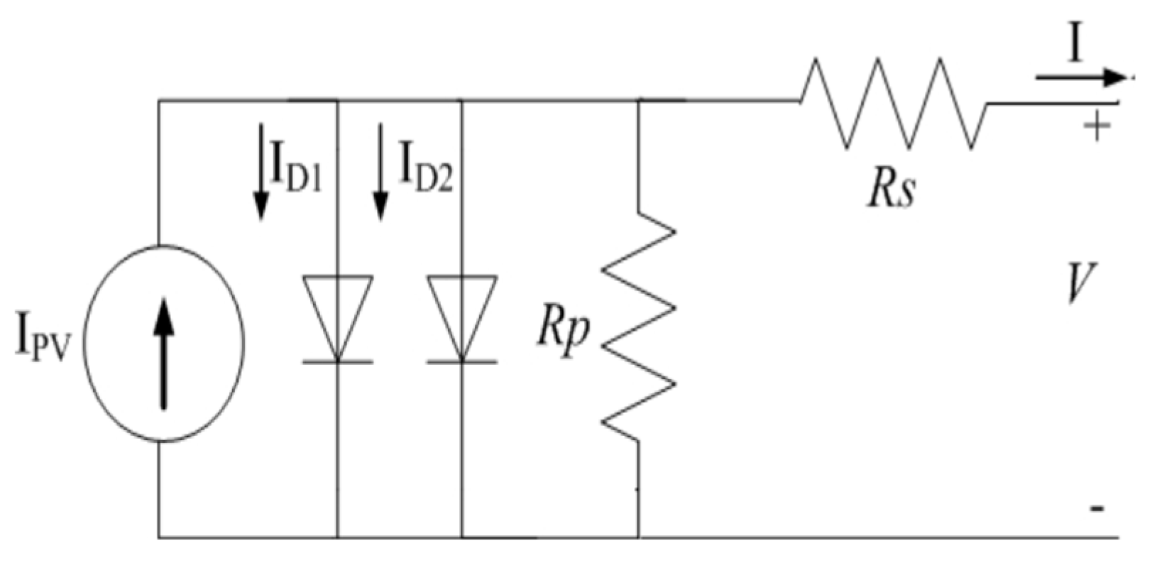
2.1. Model of the PV Cell

The PV cell has been modeled as a two-diode current source [20,22,23,26] that considers various factors, such as losses due to parasitic resistances, recombination of charge carriers, and the effects of temperature, as shown in Figure 2. The mathematical equations that govern the behavior of the PV cell can be found in the various literature [13,21,24] and have only been included here for the sake of completeness.

The following sequence of equations will calculate the final usable current of the PV cell.

$$I_{out}=I_{PH}-I_{D1}-I_{D2}-I_{RP}$$

(1)

The individual current components are given in Equations (2)–(4) and (7):

$$I_{PH}=\frac{I_{SC\_STC}+K_I\left(T-T_{STC}\right)G}{G_{STC}}$$

(2)

where T_STC is the standard operating temperature (25 °C or 298 K), G_STC is the standard irradiation (1000 W/m²), I_{SC_STC} is the short circuit current output at standard temperature and irradiation, K_I is the temperature coefficient of the short circuit current variation from standard temperature, and T and G are the ambient temperature and irradiation.

$$I_{D1}=I_{o1}\left[e^{\left(\frac{q\left(V-I\ast Rs\right)}{A_1\ast K\ast T\ast Ns}\right)}-1\right]$$

(3)

$$I_{D2}=I_{o2}\left[e^{\left(\frac{q\left(V-I\ast Rs\right)}{A_2\ast K\ast T\ast Ns}\right)}-1\right]$$

(4)

where V is the voltage across the diode, q is the electron charge (1.602 × 10⁻¹⁹ C), K is the Boltzmann constant (1.3805 × 10⁻²³ J/K), T is the junction temperature, and A₁ and A₂ are the diode ideality factors (typically A₁ is 1.3 for poly-crystalline Si), Rs is the series resistance of the PV cell, and N_S is the number of PV cells connected in series in the PV array. In the two-diode model, the value of factor A₂ is closer to 2 for the recombination process. Finally, I₀₁ and I₀₂ are the saturation currents of the two diodes given by the following equation:

$$I_{o1}=I_{o2}=I_{O,REF}\times {\left[\frac{T}{T_{STC}}\right]}^3\times e^{\left[\frac{q\ast E_g}{A\ast k}\times \left(\frac{1}{T_{STC}}-\frac{1}{T}\right)\right]}$$

(5)

where E_g is the band gap energy of Si (1.1 eV), A is A₁ or the ideality factor for silicon, and I_{O, REF} is the reverse saturation current given by the following equation:

$$I_{o,REF}=\frac{I_{S{C}_{STC}}+Ki\times \left(T-T_{STC}\right)}{[e^{\left(\frac{q\times (V_{OC}+Kv\times \left(T-T_{STC}\right))}{A\times k\times T\times Ns}\right)}-1]}$$

(6)

where V_OC is the open circuit voltage of the PV cell. The result of Equations (5) and (6) can be substituted into both Equations (3) and (4). Therefore, the only difference between Equations (3) and (4) is the ideality factor used (1.3 vs. 2), and this produces a negligible difference in the diode current. Thus, to save simulation time, we assumed I_D1 = I_D2; i.e., we only modeled the value of I_D1 and passed it through a gain of 2 to accommodate for the second diode. The following equation gives the final term in Equation (1):

$$I_{RP}=\frac{\left(V-I\times R_s\right)}{R_P}$$

(7)

where R_S is the series parasitic resistance, and R_P is the parasitic shunt resistance of the PV cell. All values of the parameters can be found from the datasheet of the PV cell or are known constants. However, the values of R_S and R_P cannot be found from datasheets. These two parameters need to be found via a Newton-Raphson iteration by iteratively changing R_S while keeping R_P constant. R_S should be changed until the voltage and current output at MPP of the simulated model matches the experimental values. The following equation can then calculate R_P:

$$R_P=\frac{V_{MP}\times \left(V_{MP}+I_{MP}\times R_s\right)}{V_{MP}\left(I_{PV}-I_{D1}-I_{D2}\right)-P_{MAX,EX}}$$

(8)

where V_MP and I_MP are the modeled MPP voltage and currents, while P_MAX,EX is the experimental MPP. By using the Newton–Raphson iteration, the values of R_S and R_P was estimated to be 0.45 Ω and 17.6 Ω, respectively. The complete parameters for the PV cell relevant to the model are listed in

Table 1. The parameters of the solar cell used in the PV cell model.

Parameter	Value
PMAX	120 W
VMP	18.2
IMP	6.95
VOC	21.9 V
ISC	7.86 A
PCS	36 (arranged as a 4 × 9 array)
Cell Type	polycrystalline silicon cell
Standard Test Conditions (STC)	1000 W/m2, PM 1.5, 25 °C

.

2.2. Model of the Battery

The battery used in the proposed system was a lead-acid cell battery and Figure 3 shows the basic model of a battery, while Equations (9) and (10) describe the discharge and charge of the battery [27,28].

$$V_{\mathit{DISCHARGE}}=E_0-\left(K\ast \frac{Q}{Q-I_T}\ast I_F\right)-\left(K\ast \frac{Q}{Q-I_T}\ast I_T\right)+L^{-1}\left(\frac{A}{\frac{1}{B\ast I_{BATT}}S+1}\ast 0\right)$$

(9)

$$V_{\mathit{CHARGE}}=E_0-\left(K\ast \frac{Q}{I_T+0.1Q}\ast I_F\right)-\left(K\ast \frac{Q}{Q-I_T}\ast I_T\right)+L^{-1}\left(\frac{A}{\frac{1}{B\ast I_{BATT}}S+1}\ast \frac{1}{S}\right)$$

(10)

where E₀ is the constant voltage (V), K is the polarization constant (Ah⁻¹) or polarization resistance (Ω), Q is the maximum battery capacity (Ah), A is the exponential voltage (V), B is the exponential capacity (Ah)⁻¹, I_BATT is battery current, I_F is the low-frequency current dynamics (A), and I_T is the extracted capacity (Ah). I_F and I_T are given by the following equations (f is the cutoff frequency (Hz), and T is the time the battery has been used):

$$I_T={{\displaystyle \int }}_0^T{I}_{BATT}$$

(11)

I_F = I_BATT ∗ 2πf ∗ e^−2πft

(12)

Table 2. Parameters of the lead-acid cell battery.

Parameter	Value
Type	Lead-Acid Cell
Nominal Voltage	12 V
Capacity	100 Ah
Internal Resistance	≈0.5 Ω
Fully-Charged Voltage	14.5 V

shows the parameters of the battery used in the prototype of the solar charger.

2.3. Model of the Controller Algorithm

The following equations describe the controller output based on the output of the PV cell and the battery voltage level:

PWM_MAX = 1.63 − V_PV ∗ 0.039

(13)

V_CHARGE = V_BAT + 2.5

(14)

V_DIFF = V_PV − V_CHARGE

(15)

PWM_DC = 1 − V_DIFF ∗ Kp|0.5 < PWM_DC < PWM_MAX
PWM_MAX|PWM_DC > PWM_MAX
0.5|PWM_DC < 0.5

(16)

The minimum duty cycle is kept at half of the V_OC because at half the open circuit voltage, the current output is close to the short circuit current (i.e., the current is as high as it can go). The maximum duty cycle of the controller output is variable and depends on the incident irradiation on the PV cell; it can vary between 65% and 95% depending on the PV cell output and the level of battery charging current. The PWM_MAX ensures that the buck converter is never 100% loaded. Finally, the proportional constant (Kp) was chosen so that the output of the synchronous buck converter is always kept 2.5 V above the battery charge level.

The value of the proportion gain, Kp, was selected to be 13 to optimize the SBC for the battery charging at the highest illumination. The justification of this Kp value was derived from practical data based on the output of the SBC. The error needs to be minimized for V_PV ranging from ≈17.5 V–20.0 V, and for V_BAT ranging from ≈11.5 V–14.5 V. As the output voltage of SBC is a multidimensional function (i.e., a function of two inputs: V_PV and V_BAT), minimizing the error for one of the ranges, does not reduce the error for the other range. Therefore, it was decided to minimize the error for the V_BAT range, for the V_PV level of 20.0 V. The decision to optimize for the V_PV level of 20.0 V was selected because that was the maximum output voltage of the PV cell resulting from noontime illumination, per the available lab test data. The plot below shows two things, the minimum error drops to zero with an increasing value of Kp, whereas the maximum error shows a minima at Kp = 13. Thus Kp = 13 is the optimum for this proposed algorithm as shown in Figure 4.

Figure 5 and Figure 6 show further differentiation for Kp = 12.5 and Kp = 13. The error for Kp = 12.5 was minimized when V_PV = 20.5 V, and the error for Kp = 13 was minimized when V_PV = 19.5 V. Therefore Kp ≈ 12.5–13.0 optimized the SBC to charge the battery during noontime regardless of the battery’s level of charge. However, the maximum error was encountered during low light conditions (V_PV = 17.5 V), but even that maximum error was still less than 0.5 V, which was highly desirable. Therefore, these plots justified the use of Kp = 13 for the proportional control.

Finally, the proposed PID algorithm to drive the synchronous buck converter was validated by comparing it against more established contemporary algorithms, namely the various forms of maximum power point tracking algorithms. To briefly explain, the main functional difference between the MPPT and the PID algorithms is that the MPPT will set both the current and the voltage extracted from the PV cell in such a way that the maximum power will be transferred to the load [10,11].

However, the objective of the proposed PID algorithm is not the extraction of the maximum power, but the maximum current from the PV cell, preferably by running the PV cell close to its short circuit current region; thus, the voltage output was sacrificed in favor of current. The hardware for all the MPPT algorithms required both a voltage sensor and a current sensor, whereas the proposed algorithm only required a voltage sensor. Thus, the voltage sensor did not add any extra cost to the hardware because most modern controllers and embedded systems come with inbuilt analog to digital converters, which are incredibly accurate at measuring voltages in various nodes (points) in the given hardware. On the other hand, to use the MPPT algorithm, an extra hardware module (such as the current sensor) needs to be added in series to the circuit; resulting in a more complicated and expensive design. Moreover, simulations have been carried out to verify the best performance in different solar irradiances from approximately 250 W/m² irradiance (during sunset/sunrise) to 1000 W/m² irradiance (noontime). Furthermore, it should be mentioned that the P&O algorithm used in the simulation was a generic one [29]. Figure 7 illustrates a state flowchart of the SBC control technique using: (a) the P&O MPPT algorithm, and (b) the proposed PID algorithm.

3. Design of Synchronous DC–DC Buck Converter

3.1. Design of the Synchronous Buck Converter with Filter

In this paper, a switch-mode power supply (SMPS) is proposed to provide a lower regulated output voltage than its input voltage in order to produce high current with the least power loss. Synchronous DC–DC buck converter (SBC) is a widely used type of SMPS. In the SBC system, a Metal-Oxide Semiconductor Field-Effect Transistor (MOSFET) replaces the diode to reduce the 0.5 V–1 V voltage drop across the diode, which improves overall efficiency by around 5% and more [30]. Figure 8 illustrates a closed-loop voltage mode PID-controlled SBC. The design specifications of SBC are listed in

Table 3. Design Specifications of the SBC.

Actual Meaning	Symbol	Value
Maximum input voltage	Vin	24 V
Maximum output voltage	Vo	16 V
Minimum switching frequency of the SBC	fsw	20 kHz
Estimated inductor ripple current (5% of inductor current)	∆i	0.4 A
Desired output voltage ripple (2% of output voltage)	∆Vo	0.25 V
Maximum output current (Vout/R)	Iout	7.50 A

.

3.1.1. Duty Cycle

The duty cycle of an SBC is defined as the ratio of the ON period of the high-side MOSFET Q_HG over the total period.

$$D=\frac{t_{HG,on}}{t_{HG,on}+t_{LG,off}}\cong \frac{V_{out}}{V_{in}}\approx 50–85\%$$

(17)

3.1.2. Inductor and Capacitor Selection

In the SBC system, the inductor L and capacitor C are used to eliminate current and voltage ripples, respectively. The values of L and C are found by using the following equations with 1.123 mH and 470 µF, respectively.

$$V_L=L\frac{di}{dt}$$

(18)

$$\Delta i=DT\frac{(V_{in}-V_o)}{L}=D\frac{(V_{in}-V_o)}{f_{sw}L}$$

(19)

$$\begin{array}{l}L=D\frac{(V_{in}-V_o)}{f_{sw}\Delta i}\\ Q=0.7783\end{array}$$

(20)

$$\Delta V_O=\frac{\Delta q}{C_o}$$

(21)

$$C_o=\frac{\Delta i}{8\Delta V_o{f}_{sw}}$$

(22)

The circuit for the SBC using PIC16F690 microcontroller was simulated using Proteus 7.0 software. The simulation model and experimental hardware setup of the proposed PID-controlled SBC system is shown in Figure 9a,b respectively. In both cases (simulation and hardware), a variable voltage source was used in place of a PV cell to test the system response to various input voltage levels. The output of the SBC depended on the battery charge level and the PV cell output, and the simulation and experimental data was compared against each other in Table 7.

3.2. Loss Model Design of the Synchronous Buck Converter

The total losses of the SBC were dependent on many factors such as the type of semiconductor devices, operating values (voltage, current, and frequency) of the converter, core influences, and PCB manufacturing technology, etc. [30,31,32,33]. However, the efficiency of a DC–DC converter significantly depends on the semiconductor losses (P_{loss_semi}) and the inductor losses (P_{loss_inductor}) [34]. Thus, the total losses in the SBC can be assumed to be:

$$P_{Total}=P_{loss\_semi}+P_{loss\_inductor}$$

(23)

During the loss model design of SBC, several factors were assumed to simplify the loss calculation. They were:

• The temperature effect on semiconductor devices was not considered. Here all the parameters were considered for 150 °C maximum junction temperature rating according to the datasheet of a FQP50N60, 60 V N-Channel MOSFET.
• The loss due to the skin effect of the inductor was also neglected.
• The parasitic capacitance loss was also neglected.

Figure 10 depicts the fundamental waveforms of the proposed SBC for the loss calculation. Based on the operation principles of the SBC, the switching circuit can be divided into three modes:

• MODE 1 [t₀ ≤ t ≤ t₂]: High-side MOSFET Q_HG is on and conduction losses $(P_{C1})$ and switching power losses $(P_{SW})$ are raised. The switching power losses $(P_{SW})$ are calculated from the overlap area of the V_DS and I_DS;
• MODE 2 [t₂ ≤ t ≤ t₃ and t₄ ≤ t ≤ t₅]: The body diode losses $(P_{BD})$ arise as a function of the dead time when both Q_HG and Q_LG are off. There are two dead-time intervals as t₂ ≤ t ≤ t₃ and t₄ ≤ t ≤ t₅, which prevent short-through;
• MODE 3 [t₃ ≤ t ≤ t₄]: Low-side MOSFET Q_LG is turned on and conduction losses $(P_{C1})$ are taking place as there is only a voltage drop, which is equal to the forward voltage of the Schottky diode D₁.

3.2.1. Semiconductor Losses

As per mode operation of SBC, the losses in the SBC’s power switches can be defined as:

$$P_{loss\_semi}=P_{Q1}+P_{Q2}+P_{BD}$$

(24)

where $P_{Q1}$ is the total power losses in Q_HG, $P_{Q2}$ is the total power losses in Q_LG, and $P_{BD}$ is the body diode losses. The total power losses in the MOSFET Q_HG are composed of conduction losses $(P_{C1})$, switching power losses $(P_{SW})$, and gate drive losses $(P_G)$ [35,36]. Therefore, the total losses in MOSFET Q_HG are:

$$P_{Q1}=P_{C1}+P_{SW}+P_G$$

(25)

On the other hand, the switching losses for MOSFET Q_LG can be ignored. Therefore, the total loss in MOSFET Q_LG is comprised of conduction losses $(P_{C2})$ and gate drive losses $(P_G)$ [35,36].

$$P_{Q2}=P_{C2}+P_G$$

(26)

The conduction losses are:

$$P_{C1}={\left(I_O\sqrt{D}\right)}^2\times R_{DS\left(on\right)}$$

(27)

$$P_{C2}={\left(I_O\sqrt{\left(1-D\right)}\right)}^2\times R_{DS\left(on\right)}$$

(28)

The switching losses are:

$$P_{SW}=\frac{\left[V_{DS\left(max\right)}(t_r+t_f)·I_{s,rms}\right]f_{sw}}{2}$$

(29)

The gate-drive losses are:

$$P_G=V_{GS}·Q_g·f_{sw}$$

(30)

The body diode losses are:

$$P_{BD}=2·V_f·\left(I_O+\frac{\Delta I_L}{2}\right)·t_d·f_{sw}$$

(31)

where the MOSFET parameters $(R_{DS\left(on\right)}$, $V_{DS\left(max\right)}$, $t_r,t_f,V_{GS}$, $Q_g$, $V_f$ and $t_d$) are taken from the FQP50N60 datasheet. $I_o$, $I_{s,rms}$, and $\Delta I_L$ are the output current, switch current, and input current ripples, respectively.

3.2.2. Inductor Losses

The inductor losses are the sum of core losses in the iron-powered toroidal core (P_core) and conducting losses in the windings of the inductor (P_cond) [34].

$$P_{loss\_inductor}=P_{Core}+P_{Cond}$$

(32)

with

$$P_{cond}=I_{L,rms}^2{R}_L$$

(33)

$$P_{core}=W_t\left(f_{sw}^{1.68}{B}_{ac}^{1.99}\right)$$

(34)

and

$$B_{ac}=\frac{L\Delta I_L}{N_t}$$

(35)

where $R_L$ = internal resistance of the coil, $W_t$ = weight of the inductor, L = core-length, and $N_t=$ number of turns.

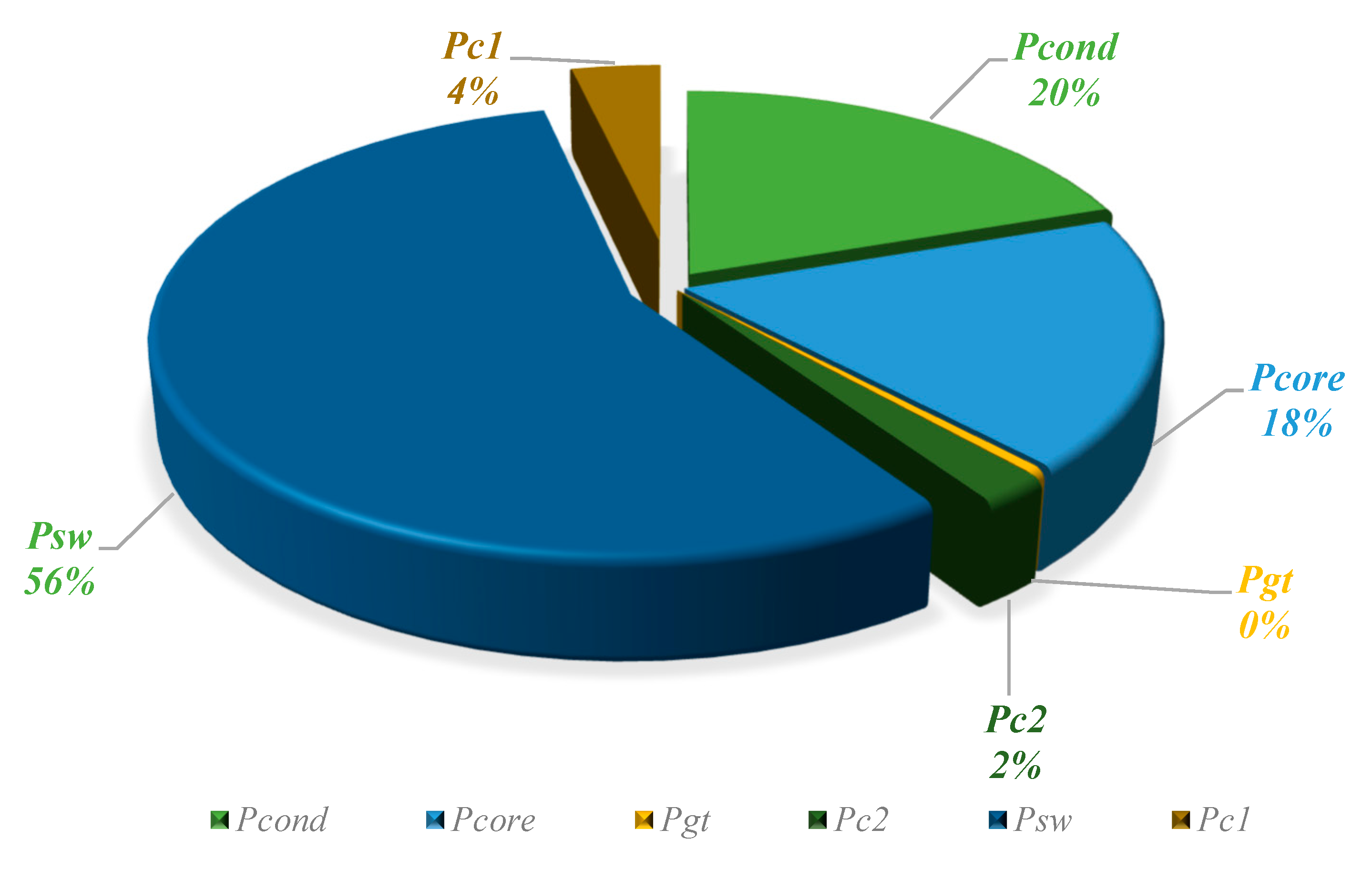
3.2.3. Total Power Losses of the SBC

The detailed distribution of power losses of the SBC is depicted in Figure 11 under a full-load condition. It can be seen from Figure 11 that the switching and conduction losses of switches have grossed 62% of the total power losses. Therefore, the switching devices needed to be chosen carefully based on $R_{DS\left(on\right)}$ of the MOSFETs to improve the converter efficiency. Also, the inductor’s core losses were found to be around 18%. Therefore, the inductor filter needed to be selected for having a minimum core loss. Moreover, the inductor conduction loss was 20%, therefore to minimize conduction loss, windings should be selected based on the available cross-sectional area.

4. Practical Implementation and Performance Evaluation

4.1. Selection of Project Location

The city of Chittagong lies at 22°22′0″ N and 91°48′0″ E [3,37]. It straddles the coastal foothills of the Chittagong Hill Tracts (CHT) in southeastern Bangladesh. The Karnaphuli River runs along the southern banks of the city, including its central business district. The river enters the Bay of Bengal in an estuary located 12 km (7.5 miles) west of downtown Chittagong [3,37]. Fishery Ghat, the largest fish market in Chittagong, is located here. This place has great significance in the economy and employment of the Chittagong district as approximately 17–19% of the total fish demand of Bangladesh is supplied from this place [38]. A large number of trawlers enter Fishery Ghat from the Bay of Bengal for trading; roughly 2000 trawlers are registered to trade here under the jurisdiction of Sadarghat Thana, Chittagong, Bangladesh. Fishery Ghat was selected for the practical implementation of this project on a fishing trawler pictured in Figure 12.

4.2. Project Installation

The team spent an entire week working on installing the proposed system on the fishing trawler. The work included surveys of forty fishing trawlers to get the dimensions of the trawlers. Then, the AutoCAD software (AutoCAD 2011, Autodesk Inc., 111 McInnis Parkway, San Rafael, CA 94903, USA) was used to design the electrical components layout within the trawler as shown in Figure 13, which shows specific locations of various components including the battery, the SBC, the light-emitting diode (LED)-lights including the light fixtures, and the signal lights. The entire electrical system was renovated with the proposed electrical components, with the exception of the electrical switchboard. Finally, the solar panel was installed and connected with the battery through the designed PID-controlled SBC-based battery charge controller system and the onboard hardware system is shown in Appendix A. The proposed system was developed for the lighting purpose; therefore, fifteen LED lights were installed throughout the trawler as listed in

Table 4. Electrical load at the proposed system.

No. of LED Bulbs	Place of the LED Bulbs	Use of the LED Bulbs
3	The front side of trawler cabin	To prepare the net before dropping into the sea To extract mature fish at night To repair net during the fishing time
2	At the upper portion of the cabin	To locate the full position of the trawler Lightening the full trawler at night time
2	Cabin room	For resting and leisure time
3	Kitchen, toilet, and engine room	To serve the specific purposes

.

4.3. System Efficiency during Field Trail

As expected, the system’s performance was found to be the most efficient around midday between 12 p.m. and 2 p.m. when the solar irradiation incident on the PV cell is the highest, as shown in Figure 14. The maximum solar irradiation occurs since the sun is positioned directly overhead, so its rays need to pass through less atmosphere to reach the PV cell. Furthermore, the sun’s rays usually are incident upon the PV cell. Therefore, it is concentrated in a small area of the PV cell instead of being dispersed, which would occur when it is incident at an angle. Both of these conditions lead to the fact that during noontime, the solar irradiation striking the PV cell is at its peak.

In this research, the traditional MPPT algorithm has been discarded in favor of a PID algorithm that maximizes the current extracted from the PV cell instead of the power. The justification for sacrificing power was to ensure that as much current was delivered to the charging battery as possible during its bulk charge phase so that it charged quicker. Therefore, the SBC operated the PV cell at around 50% of its open circuit voltage during maximum illumination, instead of the MPP voltage, which ensured that the PV cell (through the SBC) supplied close to its short circuit current (i.e., its maximum current) to the charging battery. The PID controller also maintained the voltage output of the SBC at 2.5 V higher than the battery voltage level to ensure that the direction of the charge flow was from the charger to the battery and not the other way around. The proportional gain of the controller was also tuned to deliver the maximum current during high illumination (midday) by sacrificing the current supply during low light conditions (just after sunrise and just before sunset). This was found via experimentation to be more optimal than trying to extract more current during low light conditions because that resulted in a sacrifice in the current supply during high light conditions, which was comparatively a more significant reduction.

Lastly, the system was equipped with some safety features to protect the battery including the LVD (low voltage disconnects) and LVR (low voltage reconnects). The LVD and LVR work by disconnecting the battery from the electrical load when its potential difference falls below 11.5 V, and only reconnects to the load when its potential difference rises above 12.5 V; thus, there is a 1 V hysteresis. The system also shuts down the charger when the PV cell output is below 17.5 V because this output is made during low light conditions and is not used for charging a battery. The charger is also shut down when the battery is fully charged, i.e., above 14.5 V. All this voltage operation mode algorithm is shown in Figure 7.

5. Result and Discussion

This section will present various data taken including the comparisons between the simulated and experimental results, the field trial data, and their explanations.

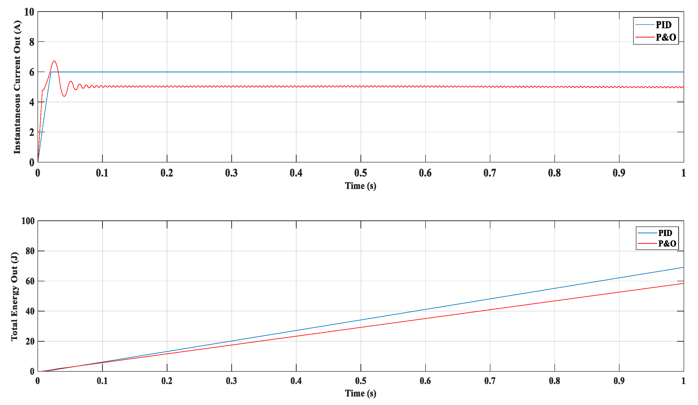
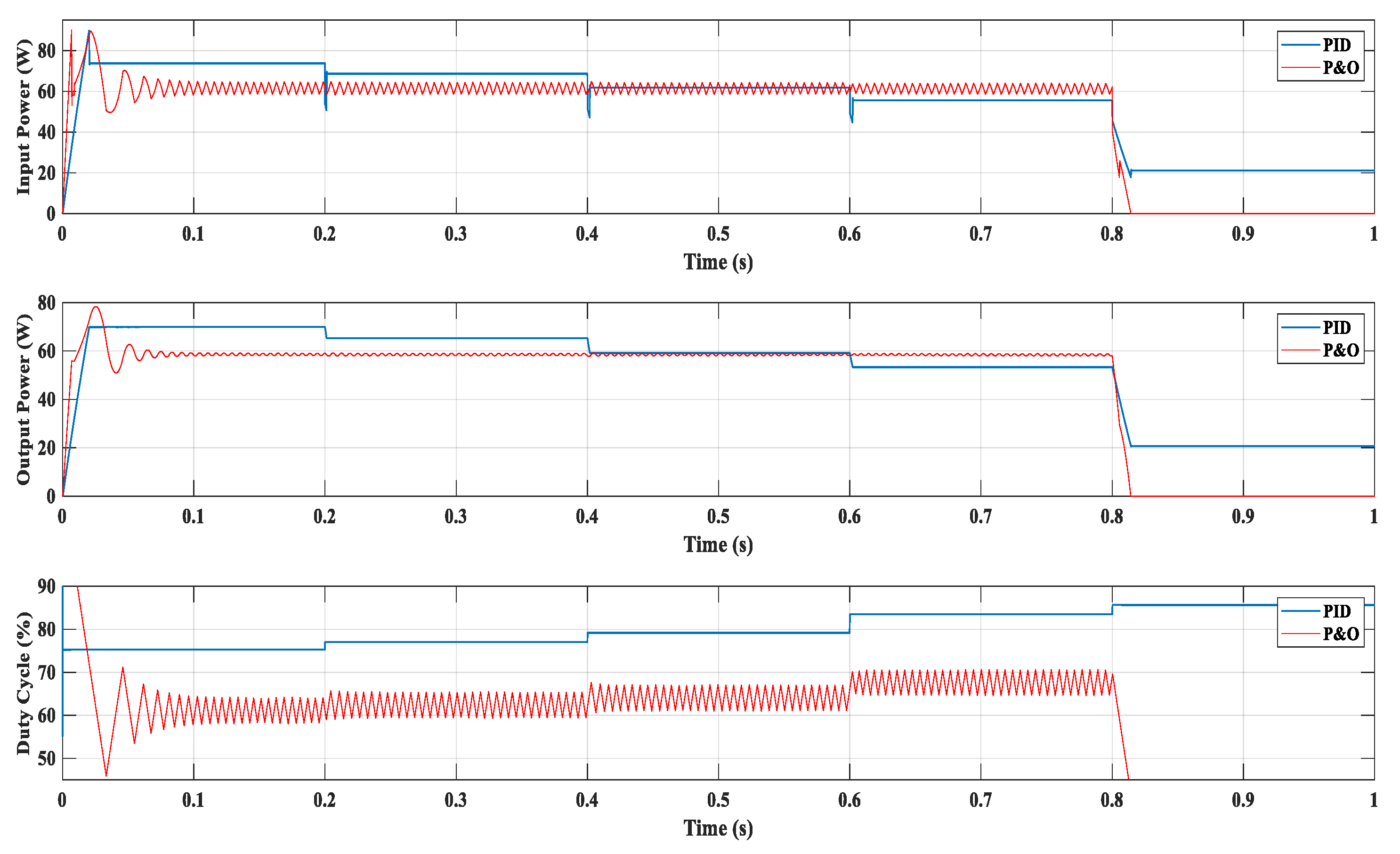
5.1. Simulation Comparison between the PID and MPPT Techniques

This section shows the simulation results of the same SBC to the proposed algorithm and a P&O MPPT algorithm. The data in

Table 5. Simulation of the SBC performance with the proposed algorithm and the P&O algorithm under various illumination condition and battery voltage level.

	Time of Day 13:30	Time of Day 14:00	Time of Day 14:30	Time of Day 15:30	Time of Day 17:00
Topology and performance parameters	Irradiance 978 W/m2	Irradiance 844.4 W/m2	Irradiance 712.9 W/m2	Irradiance 584.6 W/m2	Irradiance 264.6 W/m2
	PV cell Vout 19.90 V	PV cell Vout 19.50 V	PV cell Vout 19.00 V	PV cell Vout 18.00 V	PV cell Vout 17.50 V
	PV cell Iout 4.50 A	PV cell Iout 4.30 A	PV cell Iout 4.00 A	PV cell Iout 3.80 A	PV cell Iout 1.50 A
	Battery SoC 10.50%	Battery SoC 10.95%	Battery SoC 11.25%	Battery SoC 11.78%	Battery SoC 12.56%
	Battery Out 10.25 V	Battery Out 10.40 V	Battery Out 10.50 V	Battery Out 10.65 V	Battery Out 10.85 V
Proposed	93.3	93.8	94.4	95.1	97.6
Algorithm (%)
Proposed	66.1	62.1	56.3	51	29.9
Algorithm (J)
MPPT	93.7	94.1	94.6	95.2	96.6
(P&O) (%)
MPPT	59	55.2	50.2	44.9	24.2
(P&O) (J)

shows the comparison between the two algorithms regarding efficiency and energy output over a period of 5 s based on different PV cell outputs and battery voltage levels. These values of PV cell output and battery voltage levels have not been arbitrarily chosen, but instead, they have been taken from the field trial data presented in Table 8. The data from Time 13:30, 14:00, 14:30, 15:30, and 17:00 have been taken for simulation purpose as they cover the PV cell voltage outputs from midday till sunset.

Table 5 shows some similarities and some differences between the proposed algorithm and the P&O algorithm. The efficiencies of the two algorithms were very similar, with the P&O algorithm showing a slightly better efficiency (+0.4%) than the proposed algorithm when the solar irradiance was at its maximum at midday. Furthermore, the efficiencies of both algorithms increased as the solar irradiance decreased. However, the efficiency of the proposed algorithm showed a higher rate of increase than the P&O algorithm, with the efficiency of the proposed algorithm catching up to the efficiency of the P&O algorithm towards afternoon, and eventually overtaking it in the evening. Overall, the differences in efficiencies were too little to differentiate the performance of the proposed algorithm from that of the P&O algorithm; except in the evening when the proposed algorithm was 1% more efficient than the P&O algorithm. As for the energy output, the proposed algorithm gave a higher lead of approximately 6–7 J over the P&O algorithm throughout the day.

Figure 15 shows several simulation plots that validate the much smoother transient performance of the proposed algorithm compared to the continuously oscillatory performance of the P&O algorithm. It also shows that the proposed algorithm has a slight advantage over the P&O algorithm in that the transients were eliminated quickly, whereas in the P&O there was a continuous oscillation seen in various outputs. Furthermore, the proposed algorithm depicted a slightly faster battery charging than the P&O algorithm. This may be due to the higher current output when using the proposed output.

Figure 16 shows the response of both algorithms, in power and control outputs, to changes in the irradiance from 978 W/m² to 264.6 W/m². The irradiance, which was 978.0 W/m² (midday) initially, changed to 844.4 W/m² at 0.2 s, 719.2 W/m² (afternoon) at 0.4 s, 584.6 W/m² at 0.6 s, and 264.6 W/m² (evening) at 0.8 s. The controller implementing the P&O algorithm was good at keeping the power levels constant throughout the day at 60 W. The proposed algorithm, on the other hand, changed the power output based on the irradiance incident on the PV cell. Therefore, the power level was the highest during midday and decreased as the day progressed to afternoon, and then to evening. Before afternoon, the proposed algorithm outperformed the P&O algorithm in charging the battery. The P&O algorithm was also unable to maintain the MPP level when the output of the PV cell decreased to a very low value, and thus the P&O controller failed to converge, resulting in zero output power. However, the proposed algorithm could keep charging the battery even at low power levels. Thus, the battery can be charged right until sunset using the proposed algorithm. Simulation results comparing the proposed algorithm to a popular MPPT algorithm shows a more favorable performance by the proposed algorithm as it offered a faster battery charging due to a higher current output, a quicker elimination of transients due to a sudden change in solar irradiance, a lack of oscillation evident in many MPPT algorithms, and also the ability to charge the battery during low light conditions.

Finally, in

Table 6. Features comparison among the PID and MPPT techniques.

	Features	Sensor	Control	Speed	Stability	Circuit Type	Cost
Techniques
Proposed PID Method		1	Simple	Medium	Stable	D	Low
P&O Method [29,39]		2	Medium	Slow	Not Stable	A/D	Medium
INC Method [9]		2	Medium	Slow	Not Stable	A/D	Medium
Fuzzy Logic Method [40]		2	High	Fast	Highly Stable	D	High
ANN Method [41,42]		2	High	Very fast	Highly Stable	D	High

A = Analog circuit, D = Digital circuit.

, the proposed algorithm is compared with frequently used MPPT techniques based on different performance features, such as the number of required sensors, applied control technique, the speed of tracking process, the stability of the system, types of circuity, and approximate implementation cost. In comparison with different MPPT techniques, the proposed method could be selected as a good solution for a standalone-PV application connects with the battery charging system for faster charging, stable operation, simple control architecture, and lower price.

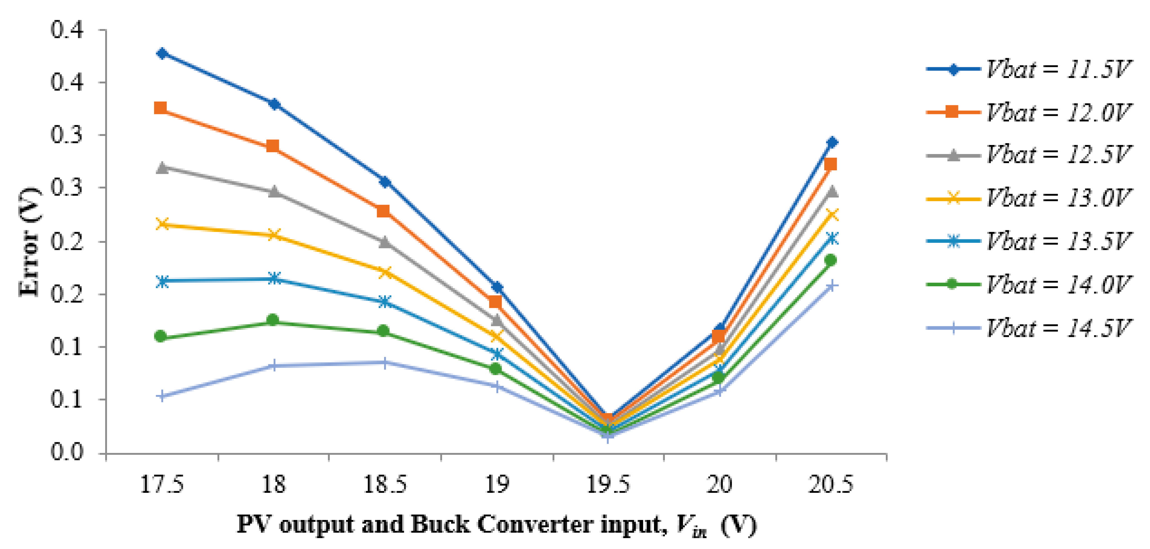
5.2. Comparison between the SBC Hardware and Simulation

These results obtained from the simulation of the mathematical model is compared with the results obtained from the hardware prototype. The complete system including the PV cell, the SBC, the microcontroller, and the battery was simulated using the Proteus software 7.0. The Proteus software 7.0 has the advantage that it uses SPICE for all electrical simulations resulting in more accurate model behavior. The simulated model is shown in Figure 9a.

Since Proteus 7.0 did not have a model of the PV/solar cell, instead of downloading a readymade PV cell library, it was decided to construct the two-diode model of the PV cell in Simulink. The voltage information gained from a simulation of the Simulink model was then configured as the V1_SOLAR value in Proteus, and the Proteus model was simulated. The results of the simulation and the prototype are compared in

Table 7. Comparison of simulation and hardware result.

PV Output (V)	Battery Level (V)	Hardware		Simulation
		PWM (%)	Buck (V)	PWM (%)	Buck (%)
25	13.3	64	15.5	60.5	15.0
	13	61	15.2	59.2	14.8
	12.5	59	14.7	56.4	14.1
	12	57	14	54.4	13.6
	11.5	54	13.5	52.4	13.1
	11	52	13	50.4	12.5
	10.6	50	12.7	48.4	12.1
Average deviation between hardware and simulation					0.49 V
24	13.3	67	15.8	64.4	15.4
	13	66	15.6	63.6	15.2
	12.5	64	15	60.4	14.5
	12	61	14.6	59	14.1
	11.5	59	14	56.6	13.6
	11	57	13.5	54.4	13.1
	10.6	54	13	52.8	12.7
Average deviation between hardware and simulation					0.42 V
23	13.3	71	16	68.8	15.8
	13	70	15.9	68	15.6
	12.5	68	15.3	64.8	15
	12	66	14.9	63.2	14.5
	11.5	64	14.3	60.8	14
	11	61	13.8	59	13.5
	10.6	59	13.5	57	13.2
Average deviation between hardware and simulation					0.32 V

, which shows the control output (in PWM duty cycle) of the microcontroller, and the buck converter output for different PV cell outputs and battery charge levels.

From Table 7 above, the output of the buck converter was approximately 0.3–0.5 V higher in the hardware prototype than in the simulation. This systemic error can be explained if we consider that the sensor that is responsible for monitoring the battery charge level was reading a higher voltage level than the actual one. However, the error was small enough that it did not affect the overall system performance.

5.3. The Field Trial Data Analysis

The field trial was conducted on a two-week period with the complete hardware retrofitted into a fishing trawler. The trawler spent the entire time in the Bay of Bengal. Various readings were taken at half-hour intervals over the two-week period. The data is presented in

Table 8. Two-week field trial data presented as average values in half-hour intervals.

Time	Vin	Iin	Pin	Vo	Io	Po	η%
6:00	16.50	0.30	4.95	0	0	0	0
6:30	17.50	0.80	14.00	12.20	0.90	10.98	78.4
7:00	17.50	0.85	14.88	12.20	0.95	11.59	77.9
7:30	17.80	0.90	16.02	12.30	1.10	13.53	84.5
8:00	18.00	1.10	19.80	12.30	1.30	15.99	80.8
8:30	18.00	1.50	27.00	12.30	1.80	22.14	82
9:00	18.50	1.50	27.75	12.30	1.80	22.14	79.8
9:30	18.50	1.70	31.45	12.40	2.00	24.80	78.9
10:00	18.50	2.00	37.00	12.40	2.40	29.76	80.4
10:30	18.50	2.50	46.25	12.45	3.00	37.35	80.8
11:00	19.00	3.00	57.00	12.50	3.70	46.25	81.1
11:30	19.00	3.50	66.50	12.55	4.40	53.97	81.2
12:00	19.50	4.00	78.00	12.60	5.50	69.30	88.8
12:30	19.79	4.50	89.06	12.65	6.30	79.70	89.5
13:00	19.90	4.50	89.55	12.70	6.50	82.55	92.2
13:30	19.90	4.50	89.55	12.75	6.40	81.60	91.1
14:00	19.50	4.30	83.85	12.90	5.60	72.24	86.2
14:30	19.00	4.00	76.00	13.00	5.00	65.00	85.5
15:00	18.85	4.00	75.40	13.10	4.80	62.88	83.4
15:30	18.00	3.80	68.40	13.15	4.30	56.55	82.7
16:00	17.75	3.50	62.13	13.25	3.90	51.68	83.2
16:30	17.70	3.30	58.41	13.30	3.60	47.88	82
17:00	17.50	1.50	26.25	13.35	1.60	21.36	81.4
17:30	17.50	1.00	17.50	13.40	1.00	13.40	76.6
18:00	17.00	0.50	8.50	0	0	0	0

, and its explanation is illustrated via two plots presented in Figure 17 and Figure 18.

Figure 17 shows that as the output voltage of the PV cell increased during noontime due to increased solar irradiation, it was possible to increase the current output of the SBC by widening the ratio between the PV cell outputs to the SBC output. Accordingly, the current output of the SBC was the highest (6.3–6.5 A) when it was operating at or below 60% of the PV cell output. From the datasheet of the PV cell, 7.86 A was the stated short-circuit current, which means that it is the highest current the PV cell can output when it is fully irradiated and operating under short-circuit conditions. Thus, using the approach outlined in Section 2.3, and the algorithm in Equation (16), the SBC was able to deliver close to the maximum possible current to charge the battery.

The highest output voltage of the PV cell during the 15-day trial period was 20 V, whereas, in the datasheet, its stated open circuit voltage under maximum irradiation was 21.9 V. To explain the variation, it was hypothesized that the PV cell was never entirely irradiated during field test conditions due to various reasons, the chief among them being that it was monsoon season in the Bay of Bengal where the fishing trawlers were based. Thus, there was always above-average cloud cover resulting in lower solar irradiation. If the PV cell was fully irradiated, the PID control algorithm could have operated the SBC so that its voltage output was only 50% of the PV cell voltage output; this would have resulted in an even higher current output from the buck converter, approaching the short circuit current of the PV cell, resulting in the highest rate of charging of the battery. Another fact that can explain the reduced voltage output is that the PV cell was not truly operating under open circuit conditions when it was connected to the SBC. The SBC acted as a load with a finite impedance, albeit a very high impedance load, so the PV cell output measured by the voltmeter, during its operation, was slightly less than its open circuit voltage.

Figure 18 shows the voltage charging rate of the battery. First, it should be noted that the battery charge level was measured at intervals of half an hour, so the rate of charging was twice the difference of the battery charge level between measurements. Second, the battery remained in the bulk charging phase throughout the experiment, thus its resistance to charging was low resulting in a higher charging rate. At higher charge levels, the resistance of the battery to charging increased, resulting in a lower charging rate for the same current input. The figure shows that the current output of the buck converter was related to the rate of charging of the battery. Increasing the current output of the buck converter translated to a higher voltage charging rate, as shown by the fact that the increase in battery voltage over time tripled from 0.1 V/h to 0.3 V/h once the current input to the battery doubled from 3 A to 6 A. Next, the plot also showed that there was a “charging inertia” of the battery. This was deduced from the fact that the battery “resisted charging,” or is extremely slow to charge initially unless the current supplied to the battery increased beyond 2 A. However, once charging started, the battery continued charging even with a low input current. This charging inertia also ensured that the battery needed a sustained charging current of above 6 A for an hour before the rate of increase of its voltage reached a peak. The change in the charging rate was not instantaneous even though the current output of the buck converter varied rapidly throughout the day. Finally, the charging inertia showed itself as “charging momentum,” which could be deduced from the fact that the battery kept its rate of voltage increase constant even though the current supply to the battery rapidly decreased from 4 A to below 2 A over a two-hour period leading to sunset.

5.4. Synchronous Buck Converter Efficiency Verification

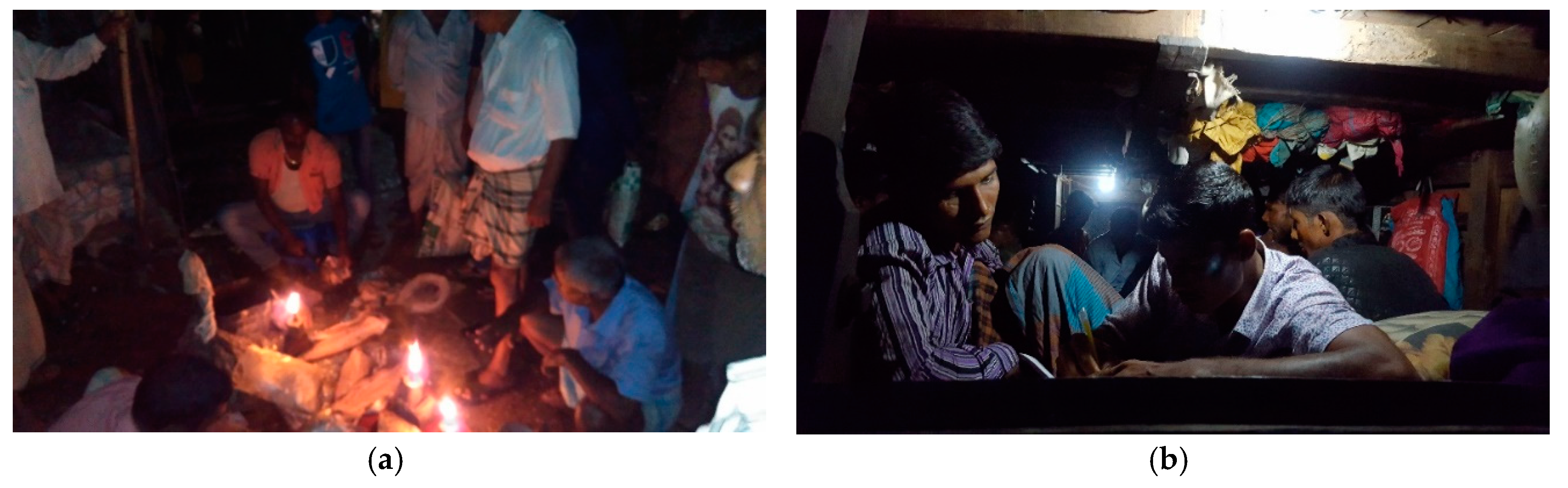
The efficiency comparison between the analytical model and experimental result is depicted in Figure 19. Here, the efficiency evaluation of the SBC considered the variation of both input voltage and load for a fair comparison with field test data. As the power level of the field test data changed remarkably from 30 W to 80 W, the analytical model results were also within that power range. It was observed that in both cases, the efficiencies were found to be around 80–92% for an output power range from 30 W to 80 W. It can be seen from the Figure 19 that the efficiency curve of the experimental model follows the analytical efficiency curve successfully. The highest deviation between analytical model and experimental result was 3.84% at 54 W. The resultant deviation between these two models may have been caused by several errors and unmeasured losses such as measurement error, equipment error, the PCB losses, connectors’ losses, and so on. Moreover, it was observed that in both cases, the efficiency increased with higher output power, which confirmed that the converter operated with higher efficiency at or near full load.

5.5. Social Impact

Usually, when the fishing trawlers stay in the Sadarghat area for 5–10 days in between trips, they usually used kerosene oil-based lamps for scheduled works at night (i.e., fish processing, cooking, and net repairing). During this period, the trawlers engines are shut down to conserve fuel. Therefore, the batteries are not charged, which is terrible for the battery life cycle and charging conditions. Fishers know this fact, but they wish to save money, so all the electrical systems remain switched off during this time. Using our proposed system based on solar light that is free, the lighting system is able to remain on in between trips because the lights themselves are energy efficient LED bulbs that draw decidedly less current from the battery. Therefore, a fully-charged battery can support the entire electrical system throughout the night and can get charged during the daytime. The proposed system thus brings a positive change in the living standard of the fishermen. Figure 20 illustrates a comparison in the living standard of the fishermen using the solar system over a conventional system.

5.6. CO₂ Reduction in the Proposed System

The present electrical system emits GHG (CO₂) that affects the environment badly. As 1 L of diesel produces 2.7 kg of CO₂. To alleviate this, the proposed system reduced the use of diesel by 450 L diesel/trawler/year [43]. This was calculated on the basis of the fact that each trawler makes around 15 fishing trips per year, each trip lasts on average 10 days, and each day required approximately 3 L of diesel to power the electrical system [43].

Therefore, the reduction of diesel required per trawler in 20 years by the proposed electrical system is = (450 L × 20 years) = 9000 L.

Therefore, the reduction of CO₂ produced in 20 years by the proposed system is 9000 × 2.7 = 24,300 kg. Therefore, it is proved that the proposed system has a great impact on carbon footprint. Since there are 2000 registered trawlers operating in the Fishery Ghat region of Chittagong port, the total amount of CO₂ reduced would equal to 48.6 kilotons.

6. Conclusions

The PID-controlled SBC-based solar charger was successfully installed in a fishing trawler, and the field data shows that it can operate at high efficiency. Although its maximum efficiency of over 90% was only achieved for a couple of hours during the middle of the day, its overall efficiency remained above 80% throughout its operating period during the day. In low light conditions, when its efficiency was below 80%, the SBC was powered down. This research also successfully exhibited the fact that the maximum drawing current from the PV cell was more suitable to charge a lead-acid cell battery than the maximum drawing power. Finally, comparing the simulation results with the experimental data showed a high degree of correlation between them, which verified the model that was used to define the system. The simulation of the proposed system was also compared with the simulation of a typical MPPT algorithm to verify the difference in performance between the two approaches. It was shown that the proposed algorithm outperformed the MPPT algorithm by having quicker elimination of transients due to solar irradiance change, a lack of oscillation evident in many MPPT algorithms, a higher rate of battery charging due to higher current output, the ability to charge the battery in low light conditions, and lower price. On the other hand, simulation results have demonstrated that the MPPT algorithm was more able to maintain a consistent output in the face of changing environmental conditions.

Therefore, future research can be conducted using this simulation model to expand and improve the system for the household application. The outcome of this research was a very low-cost prototype of a green energy technology that will be affordable even by the poor fishers of Bangladesh, and whose investments will see returns within two years through savings achieved from using no diesel for generating electricity to power the trawler’s electrical system and also by using no kerosene to light lamps. The proposed system also has the potential to save approximately 24,300 kg of CO₂ emissions/trawler, which indicate the immense effect on the carbon footprint.

References

1. Chakraborty, S.; Ullah, S.M.S.; Razzak, M.A. Quantifying solar potential on roof surface area of fishing trawlers in Chittagong Region in Bangladesh. In Proceedings of the IEEE Innovative Smart Grid Technologies–Asia (ISGT-Asia), Melbourne, VIC, Australia, 28 November–1 December 2016; pp. 833–837. [Google Scholar]
2. Van Mierlo, J.; Messagie, M.; Rangaraju, S. Comparative environmental assessment of alternative fueled vehicles using a life cycle assessment. Trans. Res. Procedia 2017, 25, 3439–3449. [Google Scholar] [CrossRef]
3. Hil Baky, M.A.; Rahman, M.M.; Islam, A.K.M.S. Development of renewable energy sector in Bangladesh: Current status and future potentials. Renew. Sustain. Energy Rev. 2017, 73, 1184–1197. [Google Scholar] [CrossRef]
4. Mondal, M.A.H.; Denich, M. Assessment of renewable energy resources potential for electricity generation in Bangladesh. Renew. Sustain. Energy Rev. 2010, 14, 2401–2413. [Google Scholar] [CrossRef]
5. Bhowmik, N.C. Renew Energy Cooperation-Network for the Asia Pacific. Bangladesh Renew. Energy Rep. 2009, 1, 1–36. [Google Scholar]
6. Lu, Y.; Dah-Chuan Lu, D. Analysis of a shunt maximum power point tracker for PV-battery system. In Proceedings of the 2015 Australasian Universities Power Engineering Conference (AUPEC), Wollongong, NSW, Australia, 27–30 September 2015; pp. 1–6. [Google Scholar]
7. Jordehi, A.R. Maximum power point tracking in photovoltaic (PV) systems: A review of different approaches. Renew. Sustain. Energy Rev. 2016, 65, 1127–1138. [Google Scholar] [CrossRef]
8. Saravanan, S.; Ramesh Babu, N. Maximum power point tracking algorithms for photovoltaic system—A review. Renew. Sustain. Energy Rev. 2016, 57, 192–204. [Google Scholar] [CrossRef]
9. Mankar, P.U.; Moharil, R.M. Perturb-and-Observe and Incremental Conductance Mppt Methods. Int. J. Res. Eng. Appl. Sci. 2014, 02, 60–66. [Google Scholar]
10. Esram, T.; Chapman, P.L. Comparison of Photovoltaic Array Maximum Power Point Tracking Techniques. IEEE Trans. Energy Convers. 2007, 22, 439–449. [Google Scholar] [CrossRef] [Green Version]
11. Sahu, H.S.; Nayak, S.K. Numerical approach to estimate the maximum power point of a photovoltaic array. IET Gener. Transm. Distrib. 2016, 10, 2670–2680. [Google Scholar] [CrossRef]
12. Hlaili, M.; Mechergui, H. Comparison of Different MPPT Algorithms with a Proposed One Using a Power Estimator for Grid Connected PV Systems. Int. J. Photoenergy 2016, 2016, 1728398. [Google Scholar] [CrossRef]
13. De Brito, M.A.G.; Galotto, L.; Sampaio, L.P.; e Melo, G.D.A.; Canesin, C.A. Evaluation of the Main MPPT Techniques for Photovoltaic Applications. IEEE Trans. Ind. Electron. 2013, 60, 1156–1167. [Google Scholar] [CrossRef]
14. Abdel-rahim, O.; Funato, H.; Haruna, J. Novel Predictive Maximum Power Point Tracking Techniques for Photovoltaic Applications. J. Power Electron. 2016, 16, 277–286. [Google Scholar] [CrossRef] [Green Version]
15. Thangavelu, A.; Vairakannu, S.; Parvathyshankar, D. Linear open circuit voltage-variable step-size-incremental conductance strategy-based hybrid MPPT controller for remote power applications. IET Power Electron. 2017, 10, 1363–1376. [Google Scholar] [CrossRef]
16. Shukla, J.; Shrivastava, D.J. Analysis of PV Array System with Buck-Boost Converter Using Perturb & Observe Method. Ijireeice 2015, 3, 51–57. [Google Scholar]
17. Shabrina, H.N.; Setiawan, E.A.; Sabirin, C.R. Designing of new structure PID controller of boost converter for solar photovoltaic stability. AIP Conf. Proc 2017, 1826. [Google Scholar] [CrossRef]
18. Sowparnika, G.C.; Sivalingam, A.; Thirumarimurugan, M. Modeling and Control of Renewable Source Boost Converter using Model Predictive Controller. Int. J. Comput. Appl. 2015, 5, 43–51. [Google Scholar]
19. Chiang, S.J.; Shieh, H.-J.; Chen, M.-C. Modeling and Control of PV Charger System with SEPIC Converter. IEEE Trans. Ind. Electron. 2009, 56, 4344–4353. [Google Scholar] [CrossRef]
20. Abdulwahhab, O.M. Improvement of the MATLAB/Simulink Photovoltaic System Simulator Based on a Two-Diode Model. Int. J. Soft Comput. Eng. (IJSCE) 2014, 4, 117–122. [Google Scholar]
21. Bellia, H.; Youcef, R.; Fatima, M. A detailed modeling of photovoltaic module using MATLAB. NRIAG J. Astron. Geophys. 2014, 3, 53–61. [Google Scholar] [CrossRef] [Green Version]
22. Ishaque, K.; Salam, Z.; Taheri, H. Accurate MATLAB Simulink PV System Simulator Based on a Two-Diode Model. J. Power Electron. 2011, 11, 179–187. [Google Scholar] [CrossRef] [Green Version]
23. Alrashidi, M.R.; Alhajri, M.F. Parameters Estimation of Double Diode Solar Cell Model. Eng. Technol. 2013, 7, 93–96. [Google Scholar]
24. Villalva, M.G.; Gazoli, J.R.; Filho, E.R. Comprehensive Approach to Modeling and Simulation of Photovoltaic Arrays. IEEE Trans. Power Electron 2009, 24, 1198–1208. [Google Scholar] [CrossRef]
25. Charging Information for Lead Acid Batteries. 2018. Available online: https://batteryuniversity.com/index.php/learn/article/charging_the_lead_acid_battery (accessed on 20 May 2018).
26. Talaat, Y.; Hegazy, O.; Amin, A.; Lataire, P. Control and analysis of multiphase Interleaved DC/DC Boost Converter for photovoltaic systems. In Proceedings of the 2014 Ninth International Conference on Ecological Vehicles and Renewable Energies (EVER), Monte-Carlo, Monaco, 26 June 2014; pp. 1–5. [Google Scholar]
27. Omar, N.; Monem, M.A.; Firouz, Y.; Salminen, J.; Smekens, J.; Hegazy, O.; Van Mierlo, J. Lithium iron phosphate based battery-Assessment of the aging parameters and development of cycle life model. Appl. Energy 2014, 113, 1575–1585. [Google Scholar] [CrossRef]
28. Tremblay, O.; Dessaint, L.A. Experimental validation of a battery dynamic model for EV applications. World Electr. Veh. J. 2009, 3, 289–298. [Google Scholar] [CrossRef]
29. Atiq, J.; Soori, P.K. Modelling of a grid connected solar PV system using MATLAB/Simulink. Int. J. Simul. Syst. Sci. Technol. 2017, 17, 451–457. [Google Scholar]
30. Sattar, A. DC to DC Synchronous Converter Design. IXYS Corporation, 2018. Available online: https://www.ixys.com/Documents/AppNotes/IXAN0069 (accessed on 20 April 2018).
31. Kolar, J.W.; Biela, J.; Waffler, S.; Friedli, T.; Badstuebner, U. Performance trends and limitations of power electronic systems. In Proceedings of the 6th International Conference on Integrated Power Electronics Systems, Nuremberg, Germany, 16–18 March 2010. [Google Scholar]
32. Kim, H.; Jung, Y.C.; Lee, S.W.; Lee, T.W.; Won, C.Y. Power loss analysis of interleaved soft switching boost converter for single-phase PV-PCS. J. Power Electron. 2010, 10, 335–341. [Google Scholar] [CrossRef]
33. Meng, Z.; Wang, Y.; Yang, L.; Li, W. Analysis of power loss and improved simulation method of a high frequency dual-buck full-bridge inverter. Energies 2017, 10, 311. [Google Scholar] [CrossRef]
34. Tran, D.; Chakraborty, S.; Lan, Y.; Van Mierlo, J.; Hegazy, O. Optimized Multiport DC/DC Converter for Vehicle Drivetrains: Topology and Design Optimization. Appl. Sci. 2018, 8, 1351. [Google Scholar] [CrossRef]
35. Lakkas, G. MOSFET power losses and how they affect power-supply efficiency. Analog Appl. 2016, 10, 22–26. [Google Scholar]
36. Depew, J.; Mosfet, L. AN1471, Efficiency Analysis of a Synchronous Buck Converter using Microsoft Office Excel-Based Loss Calculator. In Appl. Note; Microchip Technology Inc.: Chandler, AZ, USA, 2012; pp. 1–14. [Google Scholar]
37. Hossain, M.S.; Chowdhury, S.R.; Das, N.G.; Sharifuzzaman, S.M.; Sultana, A. Integration of GIS and multicriteria decision analysis for urban aquaculture development in Bangladesh. Landsc. Urban Plan. 2009, 90, 119–133. [Google Scholar] [CrossRef]
38. Shamsuzzaman, M.M.; Islam, M.M.; Tania, N.J.; Abdullah Al-Mamun, M.; Barman, P.P.; Xu, X. Fisheries resources of Bangladesh: Present status and future direction. Aquac. Fish. 2017, 2, 145–156. [Google Scholar] [CrossRef]
39. Francis, W.K.; Shanifa, B.S.; Mathew, P.J. MATLAB/Simulink PV Module Model of P & O and DC Link CDC MPPT Algorithms with Labview Real Time Monitoring and Control Over P & O Technique. Int. J. Adv. Res. Electr. Electron. Instrum. Eng. 2014, 5, 92–101. [Google Scholar]
40. Rezk, H.; Eltamaly, A.M. A comprehensive comparison of different MPPT techniques for photovoltaic systems. Sol. Energy 2015, 112, 1–11. [Google Scholar] [CrossRef]
41. Subudhi, B.; Pradhan, R. A Comparative Study on Maximum Power Point Tracking Techniques for Photovoltaic Power Systems. IEEE Trans. Sustain. Energy 2013, 4, 89–98. [Google Scholar] [CrossRef]
42. Karami, N.; Moubayed, N.; Outbib, R. General review and classification of different MPPT Techniques. Renew. Sustain. Energy Rev. 2017, 68, 1–18. [Google Scholar] [CrossRef]
43. Chakraborty, S.; Ullah, S.M.S.; Hasan, M.M.; Razzak, M.A. Feasibility study of solar power system in fishing trawlers in Chittagong region of the Bay of Bengal. In Proceedings of the IEEE Region 10 Conference (TENCON), Singapore, 22–25 November 2016; pp. 1294–1297. [Google Scholar]
Figure 1. I-V characteristics of a PV cell showing the constant current region.
Energies 11 02722 g001
Figure 2. A two-diode model of the PV-cell with parasitic resistances.
Energies 11 02722 g002
Figure 3. The basic model of a battery.
Energies 11 02722 g003
Figure 4. Plot showing the error between the buck output and the required charging voltage for various Kp values.
Energies 11 02722 g004
Figure 5. The buck converter output error for Kp = 12.5 for a range of battery charge levels and PV cell outputs.
Energies 11 02722 g005
Figure 6. The buck converter output error for Kp = 13.0 for a range of battery charge levels and PV cell outputs.
Energies 11 02722 g006
Figure 7. A state flowchart of SBC control technique using: (a) the P&O method, and (b) the proposed PID method.
Energies 11 02722 g007
Figure 8. Diagram of a PID-controlled synchronous buck converter.
Energies 11 02722 g008
Figure 9. (a) The Proteus 7.0 simulation model of the proposed system; (b) Experimental setup of PID-controlled SBC.
Energies 11 02722 g009
Figure 10. Fundamental waveforms of the proposed SBC.
Energies 11 02722 g010
Figure 11. The detailed power losses distribution of SBC at the full load condition.
Energies 11 02722 g011
Figure 12. Full view of the fishing trawler on which the proposed system is installed, and in the inset, the night view of the fishing trawler is given after the project implementation.
Energies 11 02722 g012
Figure 13. Full view of electrical wearing of the trawler using AutoCAD.
Energies 11 02722 g013
Figure 14. The efficiency of the system at various times during the day (measured).
Energies 11 02722 g014
Figure 15. Simulation comparison of output current and energy between MPPT (P&O) and the proposed algorithm during midday.
Energies 11 02722 g015
Figure 16. Simulation comparison of the dynamic response of input power, output power, and duty ratio between MPPT (P&O) and PID algorithms at a different irradiance level.
Energies 11 02722 g016
Figure 17. Field trial data comparing the SBC current output vs. ratio of SBC output to VOC (%).
Energies 11 02722 g017
Figure 18. Field trial data evaluating the battery voltage charging rate for various SBC charging current output.
Energies 11 02722 g018
Figure 19. Efficiency comparison between the analytical result and experimental result.
Energies 11 02722 g019
Figure 20. Daily activities using (a) the conventional system, and (b) the installed solar system.
Energies 11 02722 g020