Day-Ahead Hierarchical Steady State Optimal Operation for Integrated Energy System Based on Energy Hub

Abstract

The integrated energy system (IES) has the characteristic of energy system integrated/multi-energy coupling that involves heat, cooling, electricity, natural gas, and various other energy forms, which can maximize the synergistic effects and complementary benefits among various energy forms and their comprehensive utilization. In this paper, based on energy hub (EH), the day-ahead hierarchical steady state optimal operation for IES is discussed, in which the coupling natural gas system, electricity transmission system, and district heating system are all considered. Firstly, the model architecture of EH with diverse storage devices, renewable energy, and different energy conversion equipment is proposed and the steady state mathematical model of different energy networks in IES is developed, respectively. Secondly, the day-ahead operating cost of EH is minimized by an optimizing strategy to maximize the benefits of all kinds of energy demand users, where different types of energy power input into EH can be obtained. Then, the day-ahead optimal operation mode for IES considering minimization of operating fuel cost index is proposed via an energy management system, which provides various energy power data that are uploaded from EH. Finally, numerical results are presented to verify the effectiveness and usefulness of the day-ahead hierarchical optimal operation and steady state calculation analysis for IES, which could further illustrate that the proposed optimal operation can meet the requirements of practical engineering applications.

1. Introduction

Considering the background of energy internet and low-carbon electricity, the integrated energy system (IES) has played an important role in energy conservation and emission reduction processes [1,2,3,4]. In recent years, the concept of IES and its application have gradually become widely accepted with the rapid development and engineering application of renewable generation and a variety of energy storage technologies [1,3,4,5]. The IES is of great importance to improve energy efficiency and achieve the sustainable development of energy, therefore, in the past few years, there have been many results considering IES [1,4,5].

The district heating system, electricity system, natural gas system, plug-in hybrid electric vehicles (PHEVs) of future energy systems, and other various energy system forms are becoming tightly linked to each other in IES [5,6], in which the heat pump, diversified storage devices, combined cooling, heating and power (CCHP)/combined heating and power (CHP), power to gas (P2G), power to heating (P2H), absorption chiller, gas turbine, micro-gas turbine, gas furnace/boiler, etc., are all integrated. The energy coupling relationship is close and complex [2,6]. Energy hub (EH) is defined as an input–output port model that describes the energy, load, network switching, and coupling relationships in a multi-energy system [3,4,5]. As a new coupling method [2,4,5,6,7], EH can solve coupling problems between electric power systems, district heating systems, natural gas systems, etc. EH can play a role in mutual transformation, distribution, and storage of various types of energy, which is highly flexible. Besides, EH can adjust the output and operation states of different equipment according to different optimization objectives of the model, so as to meet the demand of corresponding loads [6,7].

Recently, there have been some results considering hybrid cold, heat, and power, or power and heat, or power and gas, or power, heat, and gas problems. In the literatures [8,9], a comprehensive simulation model was presented and the relationship between a power system and natural gas system was analyzed, which showed that there was a strong interdependence between the two systems. In a past paper [10], a probabilistic steady-state analysis of integrated heating, gas, and electricity systems was proposed. The probabilistic energy flow problem of IES considering correlated uncertainties and operation modes in wind, solar power, and heat, gas and electricity loads were formulated and solved by Monte Carlo method. A hierarchical energy management framework for a microgrid including multi-timescale battery energy storage and demand response was discussed previously [11], the aim was to optimize the system’s operation considering the uncertainty of renewable energy sources as well as the load. In another past paper [12], a robust optimization model was used to manage the combined heat and power systems through linear decision rules. In a different past paper [13], the heat load related to its temperature was modeled and controlled. Both of the latter references coordinated power load reduction, heat load control, and energy storage to enhance the efficiency and operational profitability of CCHP plants. In past studies [14,15], a robust optimization model was utilized to manage a building’s energy system with a CHP system, where the randomness of power load, heat load, and solar power generation were considered. In a past paper [16], hybrid energy solutions based on split air conditioning units were presented, and four different hybrid energy options, which could reduce overall energy consumption, were analyzed. In another past paper [17], several schemes for the coordination of power systems and gas systems were presented to improve security and economic aspects. In a past paper [18], the intermittent and combined operation of the CCHP system was considered, a robust optimal scheduling method was proposed to reduce the disturbance of uncertainty, however, only the description of the uncertainty in the scheduling cycle was considered, and the coupling problem of the uncertainty between the time period and the emergency was ignored. In different past papers [19,20], the optimal power flow problem of an energy system was studied, which had multiple EHs that integrate electricity and natural gas systems. In another past paper [21], the cold, heat, and electricity multi-energy flow optimization of microgrids involving renewable energy was studied. In a past paper [22], coordinated optimization was discussed for a combined cold, heat, and power supply system considering electricity, gas, cold, and thermal energy flows. In another previous paper [23], a mixed integer linear programming method was proposed to calculate the optimal power flow of multicarrier energy systems. A linear EH model based on state variables was presented to avoid introducing scheduling factor variables which were traditionally applied to optimal power flow problems. Furthermore, it is worth pointing out that the hierarchical optimal operation of IES is very important if energy production and consumption are to be coupled. However, to the best of the authors’ knowledge, most of the existing results pay more attention to CHP/CCHP, there are few results considering the day-ahead hierarchical optimal operation of IES based on EH, not to mention considering the scenario of the joint steady state optimal operation and unify management and scheduling of different systems at the same time, which are the main motivations of our paper.

Based on the above discussions, in this paper, for the aim of optimizing the operation of coupling natural gas systems, electricity transmission systems, and district heating systems, the hierarchical optimal operation mode considering one objective function of the day-ahead operating cost for EH based on peak–valley time-of-use power/heat prices and the other objective function of day-ahead fuel cost for IES based on EH, is proposed and solved effectively.

2. Inner Layer Modeling and Optimization

In this section, based on the EH concept, a practical engineering example of EH is presented, and the main energy conversion equipment in EH is modeled in detail firstly. Then, the inner layer optimization is proposed to carry out economic scheduling on EH.

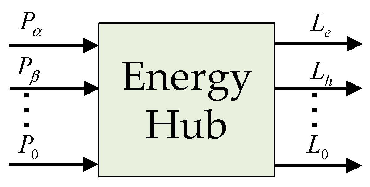
2.1. Modeling of Energy Hub

An EH integrates a variety of energy converters, such as compressors, CHP, heat exchangers, CCHP, heat recovery devices, transformers, microturbines, power-electronic devices, gas boilers, fuel cells, and other equipment, where the inputs and outputs of multiple energy flow are usually available [12,18,19]. From a system point of view, an EH is considered a unit where multiple energy flows can be converted, conditioned, and stored. This EH is also able to provide the basic features, such as input and output, conversion, and diversified storage of different energy forms [7,10,17,18,19].

A general model showing couplings with multiple inputs and outputs is illustrated in Figure 1. A unit is structured where multiple inputs are converted into multiple outputs [7,19,21]. This conversion can either be established by a single device or by a combination of multiple converters, it follows from Figure 1 that:

$$\underset{L}{\underbrace{\left[\begin{array}{c}{L}_e\\ L_h\\ ⋮\\ L_0\end{array}\right]}}=\underset{C}{\underbrace{\left[\begin{array}{cccc}{C}_{\alpha \alpha }& C_{\beta \alpha }& \cdots & C_{0\alpha }\\ C_{\alpha h}& C_{\beta h}& \cdots & C_{0h}\\ ⋮& ⋮& \ddots & ⋮\\ C_{\alpha 0}& C_{\beta 0}& \cdots & C_{00}\end{array}\right]}}\underset{P}{\underbrace{\left[\begin{array}{c}{P}_{\alpha }\\ P_{\beta }\\ ⋮\\ P_0\end{array}\right]}}$$

(1)

where L and P stand for the steady-state output and input powers vectors, respectively; the matrix C is called converter coupling matrix; the coupling factor C_ij defines the coupling between input and output power flow.

The economic efficiency of an EH can be achieved by optimally dispatching different energy carriers [21,22]. Real facilities that can be considered as EHs are, for example, small isolated energy systems, demonstration project parks, industrial areas (steel works, paper mills), big building complexes (schools, hospitals), and business areas (shopping malls).

Based on the planning and requirement of the integrated energy supply in a high-tech industrial development zone in north China, the EH architecture is constructed in Figure 2. The EH mainly includes wind power, various types of energy storage equipment, CHP units, P2G, P2H, etc., while three main energy systems (electrical, natural gas, and thermal) are considered as inputs of the EH, e.g., out of the industrial development zone. Electricity, steam/heat water, cold water, and gas will be allocated to the users of a high-tech industry development zone economically and reasonably through the energy conversion equipment. The various kinds of energy imported to an EH will be assigned, stored, and converted to meet the requirement of different energy end users. In the following, the main energy conversion equipment, including wind power, various types of energy storage equipment, the CHP unit, P2G, P2H, are modeled and introduced, respectively.

A wind power unit refers to small wind farms including many types of wind turbines and, in this paper, the relation between wind speed and the generated power from the wind turbine [1,3,20,24] is formulated as:

$$P_{wind}^t=\{\begin{array}{l}0v^t<v^{in}and{v}^t>v^{out}\\ P_{wind}^{nom}\cdot \frac{v^t-v^{in}}{v^{nom}-v^{in}}{v}^{in}\le v^t<v^{nom}\\ P_{wind}^{nom}{v}^{nom}\le v^t\le v^{out}\end{array}$$

(2)

where $P_{wind}^t$ denotes the power produced by the wind turbine; $v^t$ stands for the wind speed; $P_{wind}^{nom}$ represents the wind turbine rated power; $v^{in}$ represents the cut-in wind speed for the wind turbine; $v^{nom}$ stands for the wind turbine rated speed; and $v^{out}$ denotes the cut-out wind speed for the wind turbine.

In most cases, energy storage technology has been utilized in micro-grids, distributed energy systems, and multiple energy integration systems to smooth the fluctuations caused by PHEVs, renewable energy sources. The types of electricity storage mainly include battery storage, flywheel storage, pumped storage, super capacitors, and compressed air energy storage. In this paper, only the battery model is given. The heat storage and gas storage models are similar to each other [3,4,7] and not discussed in detail. The battery storage model is represented by:

$$\{\begin{array}{l}{W}_{bat}(t+1)=W_{bat}(t)(1-{\sigma }_{bat})+(P_{bat}^{cha}(t){\eta }_{bat}^{cha}-P_{bat}^{dis}(t)/{\eta }_{bat}^{dis})\mathsf{\Delta }t\\ W_{bat}(t)=W_{bat}(t+T)\\ 0=P_{bat}^{cha}(t)P_{bat}^{dis}(t)\end{array}$$

(3)

where $P_{bat}^{cha}(t)$ and $P_{bat}^{dis}(t)$ represent the charging and discharging power of the battery energy storage at time t, respectively; ${\eta }_{bat}^{cha}$ and ${\eta }_{bat}^{dis}$ are charging and discharging efficiencies of battery, respectively; $W_{bat}(t)$ stands for battery storage energy level at time t; ${\sigma }_{bat}$ presents the self-discharge lose rate of the battery energy storages; $\mathsf{\Delta }t$ is the simulation step, and the value in this paper is 1 h; T denotes optimal operation period.

The coupling relationship between the output power and the external heating power of CHP unit is called the “heat-to-power characteristic” of the CHP unit [14,24,25]. The relationship between the power output $P_{CHP}^{c_m}$ and the heat output $H_{CHP}^{c_m}$ of $c_m$ (a constant heat-to-power ratio) is shown in Equation (4). The alterable heat-to-power ratio, $c_z$, is considered as a variable and can be expressed by Equation (5) under a certain operating mode [5,22,25,26,27]:

$$c_m=H_{CHP}^{c_m}/P_{CHP}^{c_m}$$

(4)

$$c_z=H_{CHP}^{c_z}/({\eta }_e{F}_{in}-P_{CHP}^{c_z})$$

(5)

where ${\eta }_e$ is the power efficiency of the extraction unit in a full condensing mode; and $F_{in}$ is the fuel input rate that is taken as a constant.

In addition, P2G technology provides a new idea for absorbing the renewable and peak-cutting and valley filling of the power grid, realizing the bidirectional flow of energy between the grid and the natural gas network [15,16,28,29]. P2G input is the power $P_{P2G}$ and output is the gas flow $f_{P2G}$, their relationship can be expressed as:

$$f_{P2G}=\frac{P_{P2G}{\eta }_{P2G}}{S_{HHV}}$$

(6)

where ${\eta }_{P2G}$ represents conversion efficiency of P2G; and $S_{HHV}$ denotes the high calorific value of synthetic natural gas.

Similarly, P2H technology can transform the PV output that is difficult to be consumed by the power grid into thermal energy for the heat network, which provides a new opportunity for the absorption of distributed renewable PV power and also the coordinates operation of the power–heat interconnection of the IES [6,24,30]. P2H refers to a ground source heat pump in this paper. The relationship between the electric power $P_{P2H}$ consumed by P2H and the corresponding thermal output $H_{P2H}$ can be expressed as:

$$\{\begin{array}{c}{H}_{P2H}=P_{P2H}{\eta }_{P2H}\\ {\eta }_{P2H}=\varphi (H_{P2H})\end{array}$$

(7)

where ${\eta }_{P2H}$ represents electrothermal conversion efficiency of P2H; the functional relationship between ${\eta }_{P2H}$ and $H_{P2H}$ can be described in terms of $\varphi (\cdot )$.

The other mathematical models of the heat recovery device, heat exchanger, and furnace/boiler unit are similar to P2H, which are omitted here due to the limited length of the paper.

2.2. Inner Layer Optimization Model

After developing the EH model, in the following, the inner layer optimization model will be presented. The optimal operation cost of an EH is generally composed of purchased electricity, heat, and natural gas cost, where electrical power is provided by the electrical transmission system, heat by the district heating system, and natural gas by the natural gas system from outside the EH. From the perspective of the industrial development zone, the objective is to minimize the total energy cost of EH through economic dispatch. Therefore, the day-ahead optimal operation aims to minimize the total energy cost, including electric cost, natural gas cost, and heat cost; the objective function can be formulated as:

$$min\sum _{type}\sum _{t=1}^T{C}_{type}^t{P}_{type}^t,type=grid,gas,heat$$

(8)

where $P_{grid}^t$ stands for the total active power injection from power grid at time t; $P_{gas}^t=G_{gas}^t$ denotes the total gas flow injection from the natural gas system at time t; $P_{heat}^t=H_{heat}^t$ represents heat power demand of EH at time t; $C_{type}^t$ are the cost coefficients at time t, $type=grid,gas,heat$.

It is noted that several constraints for the components, energy storages and converters should be taken into consideration within each EH. These constraints for the current components are provided in detail.

2.2.1. Power Balance Constraint

The first constraint that should be fulfilled is the energy balance in each EH. This constraint ensures that the sum of input powers (electricity/heat/gas) at their buses is equal to the sum of output powers (electricity/heat/gas) at the corresponding buses:

$${\displaystyle \sum E_{input}^{bus}}={\displaystyle \sum E_{output}^{bus}}$$

(9)

where ${\displaystyle \sum E_{input}^{bus}}$ and ${\displaystyle \sum E_{output}^{bus}}$ denote the sum of input and output electricity/heat/gas energies at each of the corresponding buses in both EHs as shown in Figure 2, respectively.

2.2.2. Equipment Capacity and Climbing Rate Constraints

Firstly, the actual wind power consumed by EH cannot exceed the maximum output of the wind farm at time t under the optimized operation mode:

$$P_{act}^t\le P_{wind}^t$$

(10)

where $P_{act}^t$ represents actual wind power consumed by EH at time t.

In addition, the battery storage energy level should be within a given range and meet the constraint (SOC), which is described as:

$$W_{bat}^{min}\le W_{bat}(t)\le W_{bat}^{max}$$

(11)

where $W_{bat}^{min}$ and $W_{bat}^{max}$ are the minimum and maximum limits of the battery storage energy level $W_{bat}(t)$ at time t, respectively.

The ramp rate constraints of charging/discharging the battery are given by:

$$\{\begin{array}{l}0=P_{cha}^{down}\mathsf{\Delta }t\le P_{bat}^{cha}(t+1)-P_{bat}^{cha}(t)\le P_{cha}^{up}\mathsf{\Delta }t=W_{bat}^{cap}{\gamma }_{bat}^{cha}\mathsf{\Delta }t\\ 0=P_{dis}^{down}\mathsf{\Delta }t\le P_{bat}^{dis}(t-1)-P_{bat}^{dis}(t)\le P_{dis}^{up}\mathsf{\Delta }t=W_{bat}^{cap}{\gamma }_{bat}^{dis}\mathsf{\Delta }t\end{array}$$

(12)

where ${\gamma }_{bat}^{cha}$ and ${\gamma }_{bat}^{dis}$ are ratios determining maximum and minimum levels of battery energy storage, respectively; $W_{bat}^{cap}$ denotes battery capacity; $W_{bat}^{min}$ and $W_{bat}^{max}$ represent the lower and upper bounds of $W_{bat}(t)$, respectively.

Furthermore, generally speaking, when the natural gas fuel of the CHP generation system is given, the heat power output is a definite value, and the power generation output of the gas turbine is determined by the heat power output. The heat power output and the amount of natural gas are limited as:

$$H_{CHP}^{c_m,min}\le H_{CHP}^{c_m}\le H_{CHP}^{c_m,max}$$

(13)

$$H_{CHP}^{c_z,min}\le H_{CHP}^{c_z}\le H_{CHP}^{c_z,max}$$

(14)

where $H_{CHP}^{c_m,min}$ and $H_{CHP}^{c_m,max}$ denote the minimum and maximum of the heat power output from CHP unit whose heat-to-power ratio is a constant; $H_{CHP}^{c_z,min}$ and $H_{CHP}^{c_z,max}$ are the upper and lower limits of the heat power output from alterable heat-to-power ratio CHP unit, respectively.

As P2G uses electricity and produces gas, it will have an interactive impact on both the electrical and gas networks that it is connected to. P2H and P2G have similar working principles. The operation constraints of P2G/P2H can be expressed as:

$$P_{P2H}^{min}\le P_{P2H}\le P_{P2H}^{max}$$

(15)

$$P_{P2G}^{min}\le P_{P2G}\le P_{P2G}^{max}$$

(16)

where $P_{P2H}^{min}$ and $P_{P2H}^{max}$ denote the minimum and maximum of P2H consumed electricity, respectively; $P_{P2G}^{min}$ and $P_{P2G}^{max}$ stand for the upper and lower limits of P2G consumed electricity, respectively.

It is to be noted that in the above model the interaction between electric power and heat energy is based on the operation of the P2H unit (which is a ground source heat pump) and the CHP unit, while the interaction between the electric power and gas is coupled through both P2G and CHP units, and that gas and heat interact together via furnace/boiler and CHP units in an EH. The coordinated optimal operation of electricity, heat, and gas is fully taken into account in order to meet the practical engineering application scenario.

Remark 1.

It is worth pointing out that if the proposed day-ahead steady state operating cost of EH is minimized by Equation (8), then the natural gas power, thermal power, and electrical power delivered from the natural gas system, district heating system, and electricity transmission system are set as EH’s inputs. A variety of energy demands for different terminal users can be satisfied at the same time with the minimum cost by inner layer optimization model, so as to maximize the benefits of all types of energy users. Through the inner layer optimization, the optimized multi-energy flow data (i.e., EH’s inputs) are obtained based on the day-ahead forecast for all kinds of energy demands. Furthermore, the energy management system from the industrial development zone uploads these data to the upper dispatch center.

3. Outer Layer Modeling and Optimization

The IES is one of the integrated energies and power system forms, which involves electricity, heat, natural gas, and other various energy forms [2,5,8]. It is usually composed of an electrical power system, regional district heating system, natural gas pipeline network, and other energy supply networks. Therefore, the steady state operation model of different energy networks in the IES will be developed, thus the outer layer optimization model is proposed.

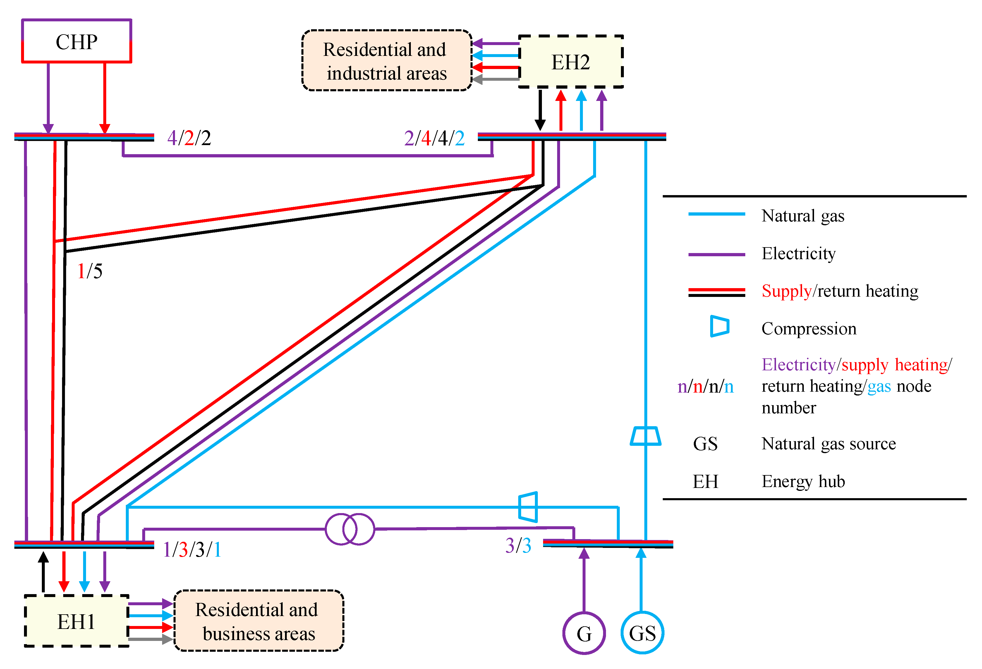
3.1. Steady State Operation Modeling of Integrated Energy System

In this section, we will consider the steady state operation model of different energy networks in the IES coupling electricity transmission system, the natural gas system, and the electricity transmission and district heating systems. The IES can be managed by the master dispatch center that coordinates and optimizes the output power of thermal generating unit, CHP plant and gas source.

3.1.1. Electricity Transmission System

Given a power system described by its electric conductance $G_{ij}$ and electrical susceptance $B_{ij}$, and given a subset of voltage, phase angle, and power injections, the power flow determines the other voltage, phase angles, active and reactive power injections [14,19,24]. The power distribution system is represented by the power balance equations at all nodes:

$$\{\begin{array}{c}{P}_i=U_i{\displaystyle \sum _{j=1}^n{U}_j(G_{ij}\cos {\theta }_{ij}+B_{ij}\sin {\theta }_{ij})}\\ Q_i=U_i{\displaystyle \sum _{j=1}^n{U}_j(G_{ij}\sin {\theta }_{ij}-B_{ij}\cos {\theta }_{ij})}\end{array}$$

(17)

where n stands for the total number of nodes; $P_i$ and $Q_i$ are the total active and reactive power injections at node i, respectively.

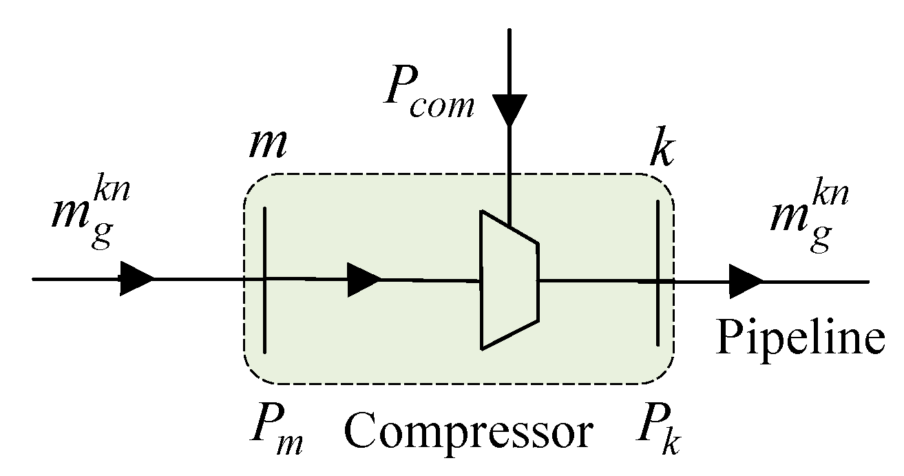
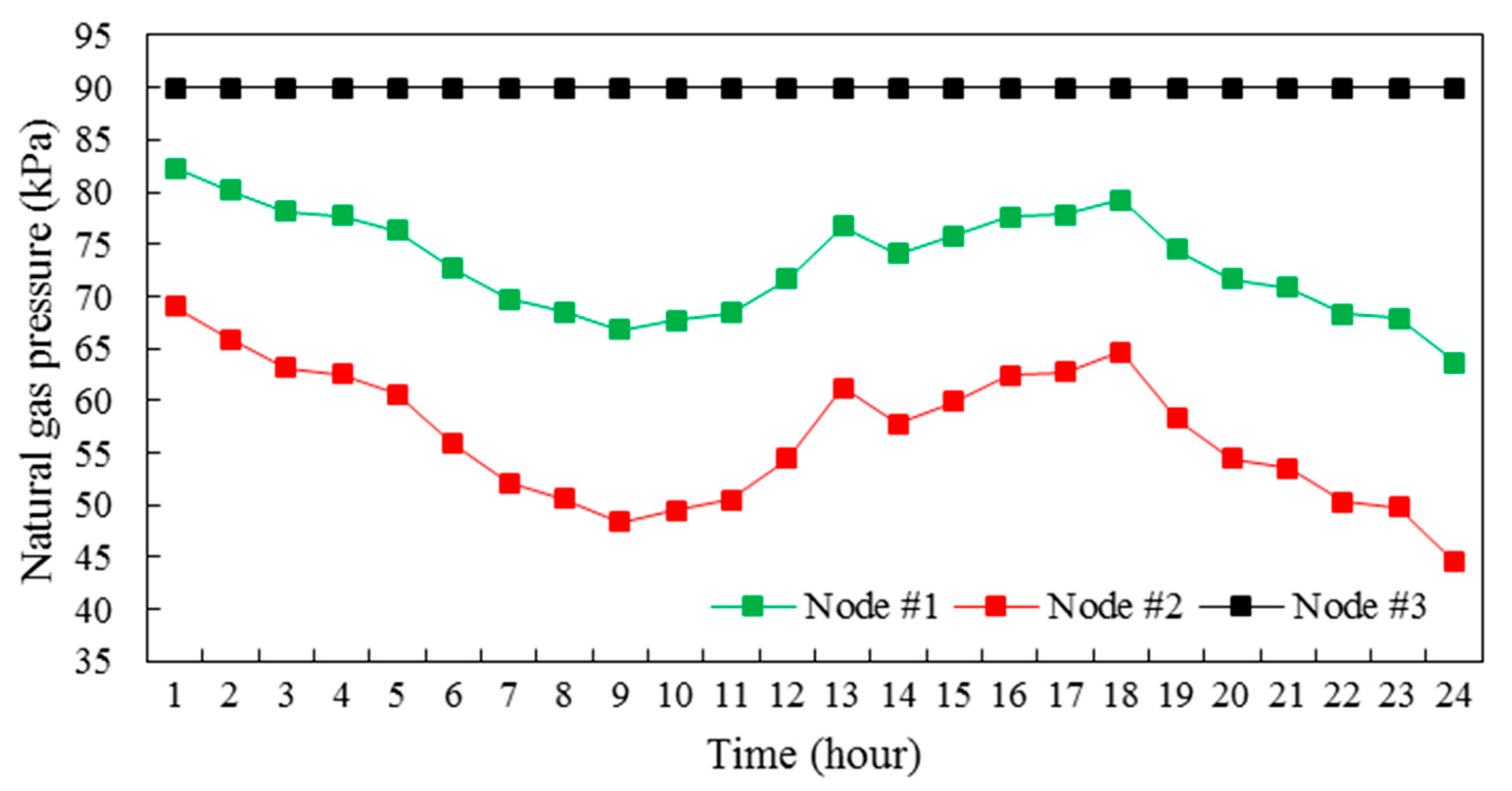
3.1.2. Natural Gas System

The steady state mode of a natural gas system can be formulated similarly to the electric power system [2,3,4,6,7,8,9]. For a gas pipeline g from node i to j, the gas flow can be expressed as:

$$\{\begin{array}{l}{m}_g={\delta }_{ij}{K}_{ij}\sqrt{{\delta }_{ij}(P_i{}^2-P_j{}^2)}\\ {\delta }_{ij}=\{\begin{array}{l}+1,P_i\ge P_j\\ -1,P_i<P_j\end{array}\end{array}$$

(18)

where $m_g$ denotes pipeline volume flow; $P_i$ and $P_j$ represent pressure at pipe start node and end node, respectively; ${\delta }_{ij}$ stands for the direction of flow in a gas pipeline; $K_{ij}$ denotes the transmission coefficient of the pipeline from bus $i$ to bus $j$, which depends on the characteristics of this pipeline.

The compressor is one of the most important components of the natural gas system, and its function is to supplement the pressure loss of the gas pipe. The electric compressor model of the gas pipe is shown in Figure 3.

$$P_{com}=K_{com}\cdot m_g^{kn}\cdot T_k\left[{(\frac{P_k}{P_m})}^{\frac{\alpha -1}{\alpha }}-1\right]$$

(19)

where $K_{com}$ denotes compression ratio; $P_{com}$ stands for the power consumption of the compressor; $\alpha$ is the specific heat ratio; $m_g^{kn}$ represents the gas flow through the compressor; and $T_k$ denotes the temperature of natural gas.

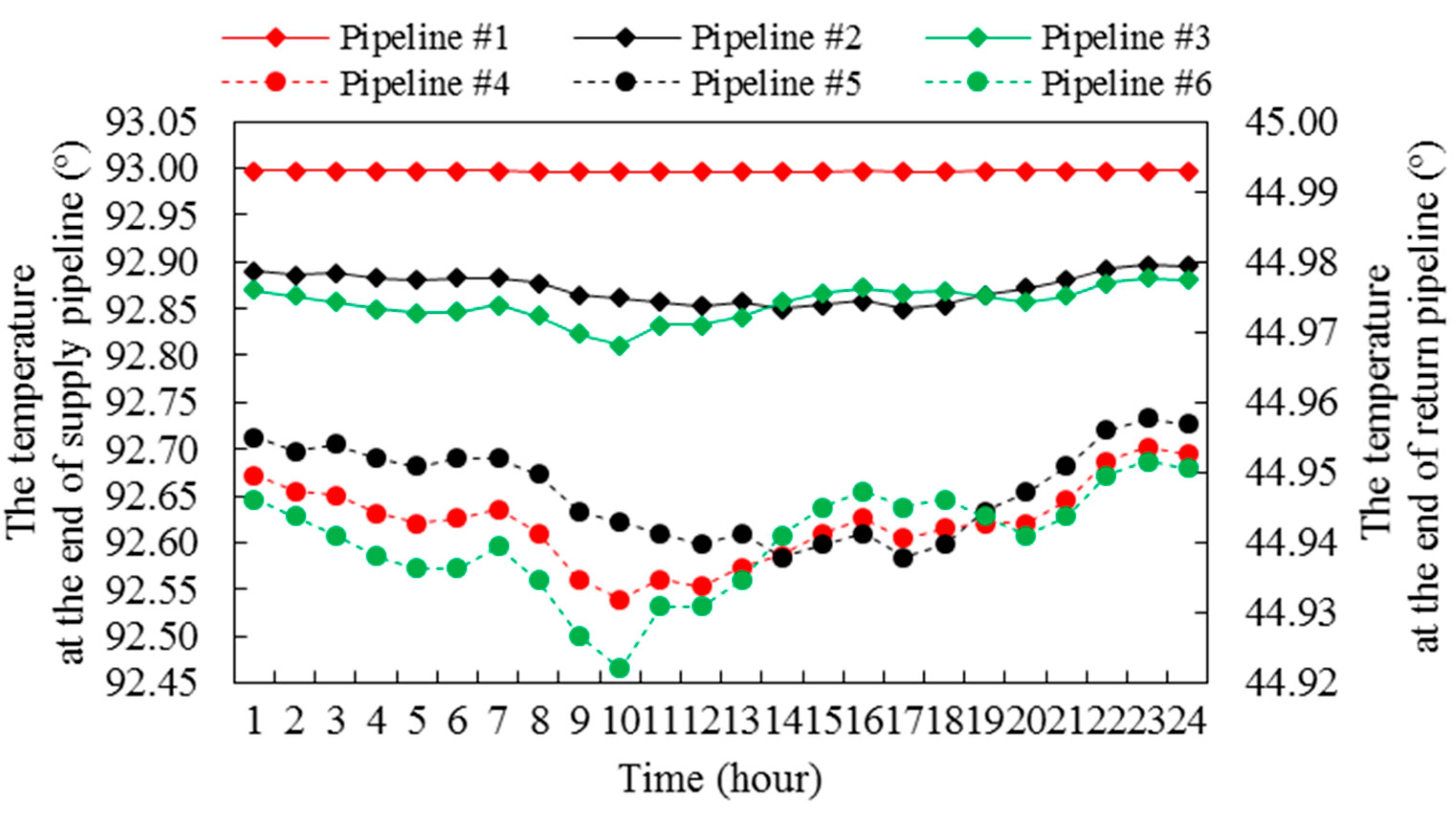
3.1.3. District Heating System

A district heating system usually consists of supply and return parallel symmetric pipelines that deliver heat energy, from the heat generation point to the end consumers. When a heat distribution system is modeled and simulated, the variables are each node pressure and each pipeline mass flow rates in the hydraulic model, correspondingly, supply and return pipeline temperatures, and transmitted thermal power in the thermal model. Model joint analysis is carried out to determine the mass flow rates within each pipe, the supply and return temperatures, and pressure at each node [8,16,25].

The continuity of flow is described as the mass flow that enters into a node such as heat load user is equal to leaving the node plus the flow consumption at the node [25]. To describe the continuity of the flow in a matrix form, the district heating system incidence matrix ${\mathbf{A}}_{\mathbf{h}}^{\mathbf{w}}$ with $n_{node}$ = $node$ rows and $n_{pipe}$ = $pipe$ columns is defined, where $n_{node}$ denotes the number of nodes and $n_{pipe}$ is the number of pipes. For the entire hydraulic network, the continuity of flow is expressed by:

$$\{\begin{array}{l}0={\mathbf{A}}_{\mathbf{h}}^{\mathbf{w}}\cdot {\mathbf{M}}_{\mathbf{h}}\\ 0={\mathbf{B}}_{\mathbf{h}}^{\mathbf{f}}\cdot (\mathsf{\Delta }{\mathbf{H}}_{\mathbf{w}}-{\mathbf{H}}_{\mathbf{p}\mathbf{u}\mathbf{m}\mathbf{p}})\end{array}$$

(20)

where ${\mathbf{M}}_{\mathbf{h}}$ is mass flow matrix composed of the mass flow ${\mathbf{m}}_{\mathbf{h}}$ within each pipe; ${\mathbf{B}}_{\mathbf{h}}^{\mathbf{f}}$ denotes the loop incidence matrix; $\mathsf{\Delta }{\mathbf{H}}_{\mathbf{w}}$ stands for the head losses within a pipe, which is the difference in head pressure ${\mathbf{H}}_{\mathbf{w}}$ between the start and end nodes within a pipe; ${\mathbf{H}}_{\mathbf{p}\mathbf{u}\mathbf{m}\mathbf{p}}$ represents the circulation pump matrix.

The pipeline diameter, pipeline length, and hot water fluid density data are assigned to each segment. The sum of all local pressure loss coefficients is assigned to each hot water supply and return pipeline, substation, and heat source plant [23,25]. The pressure drop due to friction and local losses is calculated by:

$$\{\begin{array}{l}\mathsf{\Delta }{H}_w^i=\mathsf{\Delta }{H}_f^i+\mathsf{\Delta }{H}_j^i\\ \mathsf{\Delta }{H}_f^i=\lambda \cdot \frac{L_h^i}{D_h^i}\cdot \frac{\rho v^2}{2}\\ \mathsf{\Delta }{H}_j^i=\xi \rho v^2/2\end{array}$$

(21)

where the friction coefficient $\lambda$ is specified with the corresponding hydraulic correlation; the sum of the local loss coefficients is denoted by $\xi$; the pressure drop in the heat exchange substation at the consumer end or in the heat source is described as $\mathsf{\Delta }{H}_{{}_w}^i$.

In general, the thermal model is used to determine the temperatures at start and end of each pipeline. Usually, the supply temperatures at each source and the return temperatures at each heat load user before mixing are identified in the thermal model [25,29]. The heat load user return temperature depends on the supply temperature from heat source plant, the outdoor temperature, and the heat power consumed by the heat load user. There are four different temperatures associated with each node: the supply temperatures ($T_{source}^s$ and $T_{load}^s$) and the return temperatures ($T_{source}^r$ and $T_{load}^r$). The temperature at the start of each pipeline leaving the node is equal to the mixture temperature at the same node, also, the heat power and the temperature at the outlet of a pipe are calculated by:

$$\{\begin{array}{l}{Q}_{source}^{heat}=C_p{m}_h(T_{source}^s-T_{source}^r)\\ Q_{load}^{heat}=C_p{m}_h(T_{load}^s-T_{load}^r)\\ T_{end}=(T_{start}-T_0)\exp (\frac{-{\lambda }_{pipe}{L}_h^i}{C_p{m}_h})\\ {\displaystyle \sum (m_{in}}{T}_{in})=({\displaystyle \sum m_{out}})T_{out}\end{array}$$

(22)

where $Q$ denotes the heat power consumed or supplied at each node of source or load; $T_{start}$ and $T_{end}$ denote the temperatures at the start and the end node of a pipeline, respectively; $T_0$ denotes the ambient temperature; ${\lambda }_{pipe}$ represents the coefficient of the overall heat transfer of each pipe; and $C_p$ denotes the specific heat of water for each pipe as well.

Figure 4 is a schematic diagram showing a water circulation pump, which can effectively compensate the pressure loss caused by a pipeline taking place in a district heating system. The circulating pump is usually installed at the heat source to generate and maintain the pressure difference between the supply water pipelines and the return water pipelines. However, the circulating pump is sometimes installed at some special return water pipelines to overcome the flow resistance, which meet the pressure demand of special nodes [25,27]. The power $P_{pump}$ required by the circulation pump is related to the mass flow and the static pressure difference, which is given by:

$$\{\begin{array}{l}{P}_{pump}=\frac{m_h(H_{pump}^{out}-H_{pump}^{in})}{\rho {\eta }_{pump}}\\ T_{pump}^{out}=T_{pump}^{in}\end{array}$$

(23)

where $H_{pump}^{out}$ and $H_{pump}^{in}$ are the into and out of circulation pumps pressure; ${\eta }_{pump}$ represents the working efficiency of circulation pumps; $T_{pump}^{out}$ and $T_{pump}^{in}$ stand for the into and out of circulation pumps temperature, respectively.

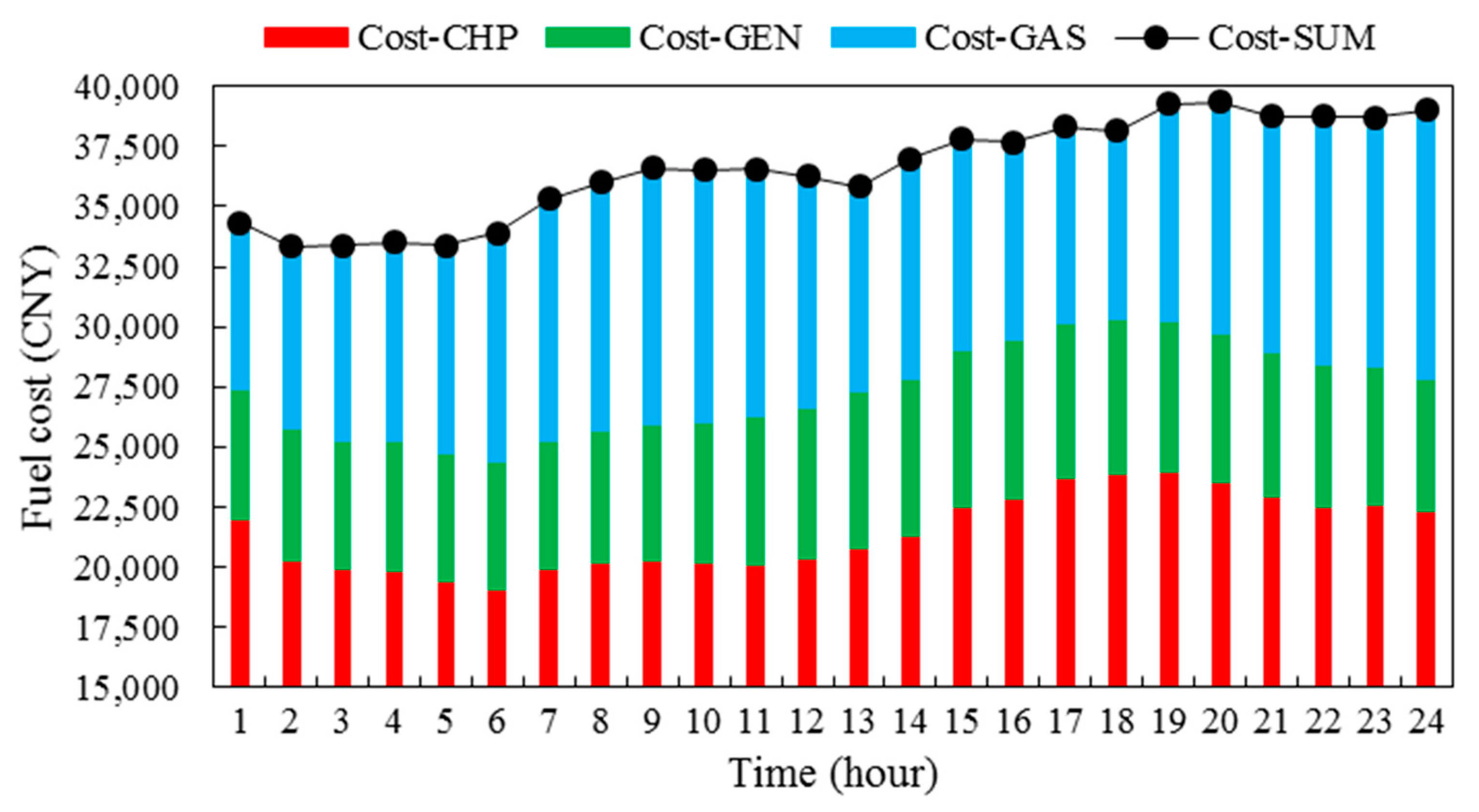
3.2. Outer Layer Optimization Model

Based on the developed steady state model of IES, the outer layer optimization model for optimal operation will be provided. For optimizing economic dispatch, the most important evaluation indices are economic [31,32,33,34]. The total fuel cost over a certain time-period of the IES can be regarded as an essential criterion for economic feasibility.

$$min{\displaystyle \sum _{source}Cos{t}_{source}},source=GEN,CHP,GAS$$

(24)

where $Cos{t}_{GEN}$, $Cos{t}_{CHP}$, and $Cos{t}_{GAS}$ denote total fuel cost of thermal generating unit, CHP unit, and gas source, respectively.

Considering the valve-point effect, the fuel cost function of each thermal generating unit is expressed as the sum of a sinusoidal and quadratic function [28,31,32,33,34]. The total fuel cost in IES over a certain period of time can be expressed as:

$$Cos{t}_{GEN}={\displaystyle \sum _{i=1}^N{\displaystyle \sum _{t=1}^T[a_i+b_i{P}_{it}^{gen}+c_i{(P_{it}^{gen})}^2+}}\left|d_i\sin \{e_i(P_{imin}^{gen}-P_{it}^{gen})\}\right|]$$

(25)

where $P_{it}^{gen}$ represents the output power of thermal unit $i$ at time t; $P_{imin}^{gen}$ stands for the lower generation limits for thermal unit $i$; $a_i$, $b_i$, $c_i$, $d_i$, and $e_i$ are the cost coefficients of thermal unit i; T represents dispatching cycle; and N is the number of generating units.

Generally speaking, CHP is known as cogeneration, and it is defined as the use of a single piece of the plant to simultaneously generate electricity and heat. The operating cost of the CHP plant is presented as follows:

$$Cos{t}_{CHP}={\displaystyle \sum _{j=1}^N{\displaystyle \sum _{t=1}^T[a_j+b_j{P}_{jt}^{chp}+c_j{(P_{jt}^{chp})}^2+}}{d}_j{H}_{jt}^{chp}+e_j{(H_{jt}^{chp})}^2+f_j{P}_{jt}^{chp}{H}_{jt}^{chp}]$$

(26)

where $P_{jt}^{chp}$ represents power generation output of CHP unit j; $a_j$, $b_j$, $c_j$, $d_j$, $e_j$ and $f_j$ are cost coefficients of CHP unit j; $H_{jt}^{chp}$ stands for heat generation output of CHP unit j.

In addition, the fuel cost function of the gas source can be expressed as:

$$Cos{t}_{GAS}={\displaystyle \sum _{k=1}^N{\displaystyle \sum _{t=1}^T(a_k+b_k{P}_{kt}^{gas})}}$$

(27)

where $a_k$ and $b_k$ denote the cost coefficients of the gas source unit k; $P_{kt}^{gas}$ represents the output power of gas source unit k at time t.

The feasible region of the outer layer optimization problem is defined by a number of constraints including different system in IES, which mainly involves limiting the variables related to network nodes and lines.

As for the electricity transmission system in the IES, the equality constraints contain the AC power flow equations, as shown in Equation (17). Inequality constraints are the active power flows through power lines, node voltage amplitudes, and the active and reactive power outputs of generators [3,25], which are generally well-known and omitted here owing to the space limit.

Furthermore, for the natural gas system in the IES, the natural gas transmission process is also subject to several constraints [3,12,19], such as pipeline volume flow limit, the compression ratio limit of each compression station, and nodal gas pressure; the constraints are formulated as:

$$m_g^{min}\le m_g\le m_g^{max}$$

(28)

$$K_{com}^{min}\le K_{com}\le K_{com}^{max}$$

(29)

$$P_n^{min}\le P_n\le P_n^{max}$$

(30)

In addition, there are also several constraints for the district heating system in the IES [3,12,25]. The mass flow rate under actual operation within each pipeline is limited and cannot exceed the design values. The heating water outlet temperature $T_{out,s}$ from the heat source should meet engineering application requirements, and the same is true for the thermal load outlet’s temperature constraints. As for the electricity-driven compressor, the power, $P_{pump}$, required by the circulation pump should be within its working capacity.

$$m_h^{min}\le m_h\le m_h^{max}$$

(31)

$$\{\begin{array}{l}{T}_{out,l}^{min}\le T_{out,l}\le T_{out,l}^{max}\\ T_{out,s}^{min}\le T_{out,s}\le T_{out,s}^{max}\end{array}$$

(32)

$$P_{pump}^{min}\le P_{pump}\le P_{pump}^{max}$$

(33)

In the above work, the steady state operation models in the IES including the electricity transmission system, natural gas system, and district heating system are developed, respectively. From the perspective of the overall IES architecture, each EH acts as a load end user, and the different systems are coupled together in a coordinated operation mode, while electricity and heat are coupled via the CHP plant, and electricity and gas are coupled together by electric compressor.

Remark 2.

The various energy power data obtained from inner layer optimization are uploaded to the master energy management system of IES. Then, the master energy management system provides various types of energy distribution information to the master scheduling center of the IES, and the dispatch center minimizes the day-ahead operating fuel cost by Equation (24), that is, outer layer optimization: achieving the economic operation saves cost.

4. Case Study

In this section, a typical winter day in north China is taken as an EH example, the energy users have typical heat, electricity, natural gas energy demands [31,32,33,34,35]. During a typical winter day, fuel cells, PHEV, solar collectors, electric chillers, and absorption chillers are not put into operation (as shown in the dotted line in Figure 2) due to insufficient sunlight intensity, extremely low demand for cold load, and the short working hours of PHEV or even no running state, etc. An IES-containing natural gas system, an electricity transmission system, district heating system, a CHP unit, a thermal generator unit, two EH units, and a natural gas source unit are presented, the structure diagram is shown in Figure 5, and the topology information of the IES case study is shown in

Table 1. Topology information of the IES case.

Electricity Transmission System	Branch/line	From node	To node
	1	1	2
	2	1	4
	3	2	4
	4	1	3
District Heating System	Branch/pipeline	From node	To node
	1	2	1
	2	1	3
	3	1	4
	4	5	2
	5	3	5
	6	4	5
	7	3	4
	8	4	3
Natural Gas System	Branch/pipeline	From node	To node
	1	3	1
	2	3	2
	3	1	2

.

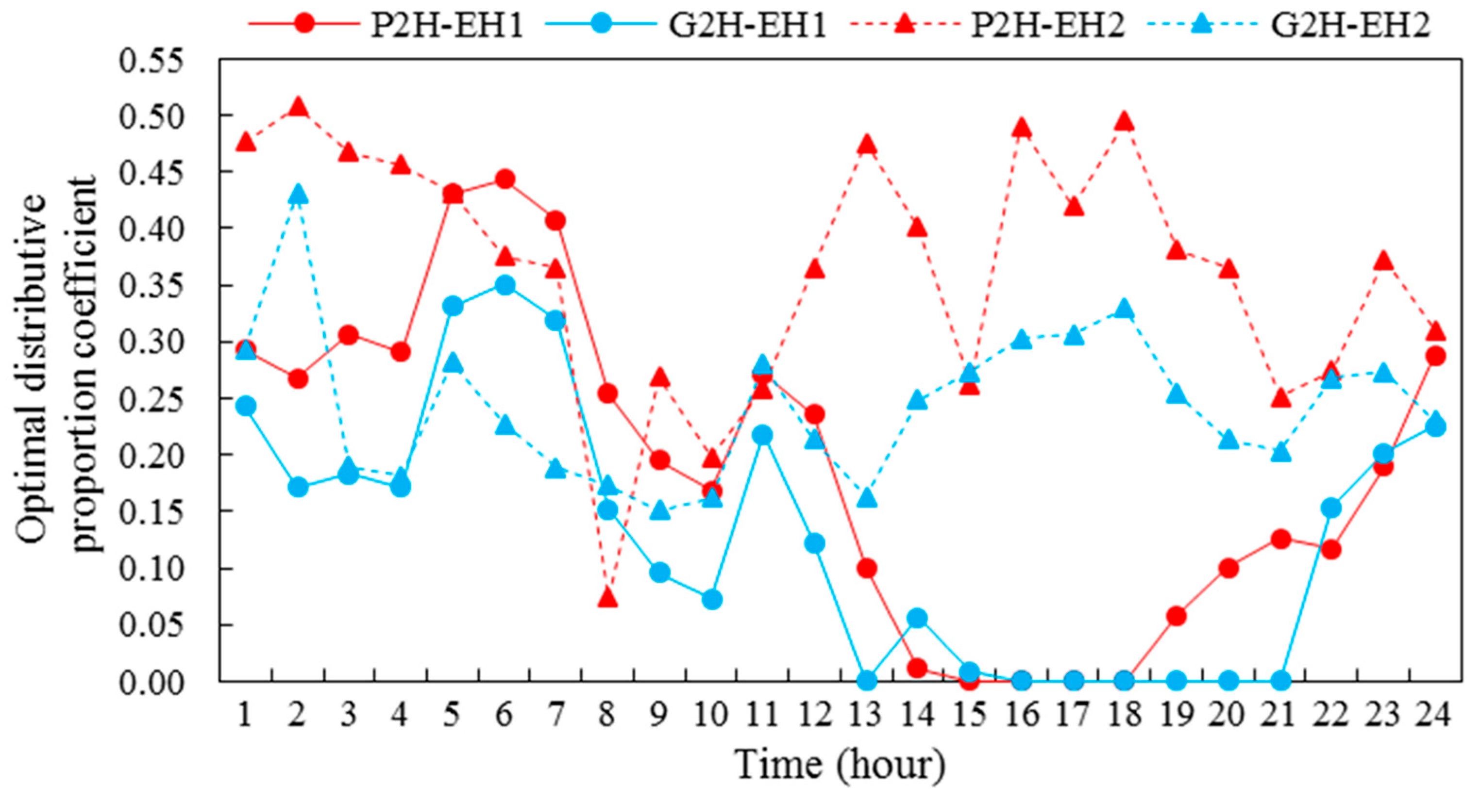
4.1. Results and Analyses

The change of battery, natural gas storage, and heat storage charge/discharge power in EH1 at a continuous time period are shown in Figure 6. During the valley price period (such as from 5:00 to 7:00), the battery is a state of charge, which can reduce the cost of electricity purchase, and also play a role in cutting peak demand (such as from 8:00 to 10:00 and from 17:00 to 18:00). However, the heat load demand is greater from 2:00 to 4:00, and heat storage, natural gas storage, and the battery are in a state of discharge so more electric energy and natural gas energy are converted to heat energy aiming to meet the heat demand peak, which reduces EH operation cost during the heat load peak period while the heat price is at the peak price. As a whole, battery, natural gas storage, and heat storage are in a state of charge from 11:00 to 16:00, meantime heat load, natural gas load, and electric load are experiencing valley demands.

As shown in Figure 2, the power proportional coefficient of total natural gas bus energy flowing to the furnace/boiler unit in EH1 is denoted as G2H-EH1, and the power proportional coefficient of total electric bus energy flowing to the P2H unit is recorded as P2H-EH1, which has the same notation in EH2. A change in the optimal distributive proportion coefficient for EH1 and EH2 in IES is shown in Figure 7. First of all, the CHP unit in EH1 and EH2 are all in the shutdown states during the whole stable operation period according to the optimization results. This can be easily understood because the CHP unit usually has a gas turbine, an internal combustion engine, or a micro-combustion machine as its main component and their energy conversion efficiency is low because of more energy loss during the energy conversion process compared to the direct use of electricity, heat, and P2H and furnace/boiler units. The results shown in Figure 7 illustrate that the optimal allocation proportion coefficient of different EHs in stable and efficient operation can be obtained by the inner layer optimization strategy. During the period from 16:00 to 18:00, the furnace/boiler and P2H units in EH1 are in the shutdown state, and the heat distribution system provides all the heat energy to meet the demand of the heat load. It can be clearly seen from Figure 7 that the variation trend of the same type curve is significantly different.

As shown in Figure 8, an electricity transmission system includes four nodes and four transmission lines, where Nodes 1 and 2 are PQ nodes, Node 3 is the PV node, and Node 4 is the slack node. Optimization results of nodes voltage magnitudes (V) and nodes voltage angles (θ) at a continuous time period are shown in Figure 8. The optimization results show that all nodes V are in the range of [0.9 p.u., 1.1 p.u.], and all nodes θ are in the range of [−8°, 0°].

The natural gas pressure at all nodes is decreased compared to the reference gas source Node 3. Figure 9 shows the pressure gradient diagram from source Node 3 to the consumer/natural gas load (from Node 1 to Node 2) at a continuous time period. Minimum pressure of the natural gas node observed under steady state is the furthest consumer (Node 2) at a continuous time period. The pressure of node 1 fluctuates up and down at 75 kPa, while that of node 2 fluctuates up and down at 58 kPa, but more violently than that of Node 1. The pressure of each node is mainly influenced by integrated factors such as EH’s natural gas load demand, natural gas pipeline flow, and pipeline resistance.

Due to the limited length, only the temperature at the end of supply/return pipeline that is connected to the supply pipeline from 1 to 3 and return pipeline from 4 to 6 in the district heating system is given. The calculation results of the supply and return pipeline’s temperatures at a continuous time period are shown in Figure 10. The results show that the temperatures at the end of the supply pipelines are approximately 92 °C, and the temperatures at end of return pipelines are approximately 44 °C. On the one hand, the temperature drop of pipelines is relatively small, and on the other hand, the temperature of heat load side is relatively stable, which can better meet the requirements of heat users.

The optimization result of day-ahead optimal operating fuel cost is 877,653.58 CNY in the IES case, and the different types of fuel cost are shown in Figure 11 at a continuous time period. The change trend of various types of fuel costs per hour is noncorrespondence with the change trend of natural gas load, heat load, and electrical load demand. Since the CHP unit undertakes the main heating supply and part of the electricity supply, the CHP unit’s fuel cost (Cost-CHP) is nearly at maximum. The output of the thermal generating unit is relatively stable, and the fuel cost (Cost-GEN) is also relatively stable, which corresponds to the operation characteristics of the thermal generating unit. The price of heat and electricity is variable, while the price of natural gas is unchanged. From the results in Figure 11, it can be seen that natural gas plays a role of peak shaving and valley filling to a certain extent, so the fuel cost of natural gas (Cost-GAS) is relatively large.

4.2. Discussions

The charge/discharge of the battery, natural gas storage, and heat storage are affected by the fluctuation of diversified load demands, peak–valley time-of-use power price, and peak–valley time-of-use heat price. Therefore, the advantages and characteristics of various kinds of energy storage systems can be comprehensively employed by complementing each other, which increases the stability of the EH operation as well as the interaction and coordination of various energies. At the same time, the coordination of different kinds of energy storage devices helps to locally promote the consumption of renewable energy, because this energy consumed in EH does not need to be purchased in this paper.

In addition, compared with the traditional electric power supply, gas supply, heat supply, and cold supply, the energy conversion equipment such as the P2G, P2H, and CHP units, provides more scheduling schemes for the dispatching center, which can, in turn, offer an optimal steady state operation scheme for the EH at each time period. The flexible cooperation of various types of energy conversion equipment also increases the security of operation for industrial development zone, because when any individual energy conversion equipment fails, the energy required by the end user is not affected due to multiple supply channels. The operation mode of EHs can be changed and adjusted flexibly according to the optimal allocation proportion coefficient. At the same time, the optimal allocation proportion coefficient provides guidance for equipment capacity selection, equipment operation time, energy conversion equipment combination mode and so on.

Furthermore, in a certain region, the coordinated operation of different energy systems through the master dispatching center in order to dispatch CHP plant, traditional thermal generating unit and natural gas source powers can ensure the most economically operated fuel cost for IES. Simulation results show that, on the one hand, the electricity transmission system has good stability in a day-ahead optimal operation, and on the other hand, the pressure of each node in the natural gas system fluctuates up and down in a reasonable and safe interval, which further indicates that optimal scheduling means that the natural gas system in a stable operation state. Meanwhile, the pipeline’s temperature fluctuation is small under a day-ahead optimal operation, which also indicates that the district heating system has good stability. It has been proven that the proposed day-ahead hierarchical steady state optimal operation for IES is feasible, effective, and reasonable.

5. Conclusions

This paper presented a day-ahead hierarchical optimal operation model for IES coupled natural gas network, electricity transmission network and district heating network based on so-called EH. The day-ahead operating cost of EH was minimized via the interior optimization strategy, maximizing user benefits of energy demand. The optimal operation mode for the IES considering minimization of the operating fuel cost index was proposed, and an outer optimization strategy maximized the benefits of energy producers. Finally, simulation results have verified the validity of the day-ahead hierarchical optimal operation and steady state calculation analysis for IES. The optimization results showed that the charge/discharge of the battery, natural gas storage, and heat storage in EH were affected by the fluctuation of diversified load demands and peak–valley time-of-use power/heat price. The combined analysis had the ability to calculate the variables of the hybrid multiple energy systems, which could be used for the design and optimal operation of IES.

References

1. Gil, M.; Dueñas, P.; Reneses, J. Electricity and natural gas interdependency: Comparison of two methodologies for coupling large market models within the European regulatory framework. IEEE Trans. Power Syst. 2015, 31, 361–369. [Google Scholar] [CrossRef]
2. Clegg, S.; Mancarella, P. Integrated modeling and assessment of the operational impact of power-to-gas (P2G) on electrical and gas transmission networks. IEEE Trans. Sustain. Energy 2015, 6, 1234–1244. [Google Scholar] [CrossRef]
3. Linna, N.; Liu, W.; Wen, F.; Xue, Y.; Dong, Z.; Zheng, Y.; Zhang, R. Optimal operation of electricity, natural gas and heat systems considering integrated demand responses and diversified storage devices. J. Mod. Power Syst. Clean Energy 2018, 6, 423–437. [Google Scholar]
4. Zeng, Q.; Zhang, B.; Fang, J.; Chen, Z. Coordinated operation of the electricity and natural gas systems with bi-directional energy conversion. Energy Procedia 2017, 105, 492–497. [Google Scholar] [CrossRef]
5. Xu, X.; Jia, H.; Chiang, H.; Yu, D.; Wang, D. Dynamic modeling and interaction of hybrid natural gas and electricity supply system in microgrid. IEEE Trans. Power Syst. 2015, 30, 1212–1221. [Google Scholar] [CrossRef]
6. Qadrdan, M.; Wu, J.; Jenkins, N.; Ekanayake, J. Operating strategies for a GB integrated gas and electricity network considering the uncertainty in wind power forecasts. IEEE Trans. Sustain. Energy 2013, 5, 128–138. [Google Scholar] [CrossRef]
7. Zhang, X.; Shahidehpour, M.; Alabdulwahab, A.; Abusorrah, A. Optimal expansion planning of energy hub with multiple energy infrastructures. IEEE Trans. Smart Grid 2017, 6, 2302–2311. [Google Scholar] [CrossRef]
8. Erdener, B.; Pambour, K.; Lavin, R.; Dengiz, B. An integrated simulation model for analyzing electricity and gas systems. Int. J. Electr. Power Energy Syst. 2014, 61, 410–420. [Google Scholar] [CrossRef]
9. Martinez-Mares, A.; Fuerte-Esquivel, C. A unified gas and power flow analysis in natural gas and electricity coupled networks. IEEE Trans. Power Syst. 2012, 27, 2156–2166. [Google Scholar] [CrossRef]
10. Yang, L.; Zhao, X.; Li, X.; Yan, W. Probabilistic steady-state operation and interaction analysis of integrated electricity, gas and heating systems. Energies 2018, 11, 917. [Google Scholar] [CrossRef]
11. Fan, S.; Ai, Q.; Piao, L.; Fan, Q.; Piao, L. Hierarchical energy management of micro-grids including storage and demand response. Energies 2018, 11, 1111. [Google Scholar] [CrossRef]
12. Brahman, F.; Honarmand, M.; Jadid, S. Optimal electrical and thermal energy management of a residential energy hub, integrating demand response and energy storage system. Energy Build. 2015, 90, 65–75. [Google Scholar] [CrossRef]
13. Anvari-Moghaddam, A.; Monsef, H.; Rahimi-Kian, A. Optimal smart home energy management considering energy saving and a comfortable lifestyle. IEEE Trans. Smart Grid 2017, 6, 324–332. [Google Scholar] [CrossRef]
14. Wang, R.; Wang, P.; Xiao, G. A robust optimization approach for energy generation scheduling in micro-grids. Energy Convers. Manag. 2015, 106, 597–607. [Google Scholar] [CrossRef]
15. Wang, C.; Jiao, B.; Guo, L.; Tian, Z.; Niu, J.; Li, S. Robust scheduling of building energy system under uncertainty. Appl. Energy 2016, 167, 366–376. [Google Scholar] [CrossRef]
16. Nižetić, S.; Papadopoulos, A.; Tina, G.; Rosa-Clot, M. Hybrid energy scenarios for residential applications based on the heat pump split air-conditioning units for operation in the Mediterranean climate conditions. Energy Build. 2017, 140, 110–120. [Google Scholar] [CrossRef]
17. Zlotnik, A.; Roald, L.; Backhaus, S.; Chertkov, M.; Andersson, G. Coordinated scheduling for interdependent electric power and natural gas infrastructures. IEEE Trans. Power Syst. 2017, 32, 600–610. [Google Scholar] [CrossRef]
18. Wang, L.; Li, Q.; Sun, M.; Wang, G. Robust optimization scheduling of CCHP systems with multi-energy based on minimax regret criterion. IET Gener. Transm. Distrib. 2016, 10, 2194–2201. [Google Scholar] [CrossRef]
19. Geidl, M.; Andersson, G. Optimal power flow of multiple energy carriers. IEEE Trans. Power Syst. 2007, 22, 145–155. [Google Scholar] [CrossRef]
20. Moeini-Aghtaie, M.; Abbaspour, A.; Fotuhi-Firuzabad, M.; Hajipour, E. A decomposed solution to multiple-energy carriers optimal power flow. IEEE Trans. Power Syst. 2014, 29, 707–716. [Google Scholar] [CrossRef]
21. Lin, G.; Chen, Y.; Liu, Y.; Xiong, W.; Tang, L.; Pan, Z.; Guo, Q. Coordinative optimization of multiple energy flows for microgrid with renewable energy resources and case study. Electr. Power Autom. Equip. 2017, 37, 275–281. [Google Scholar]
22. Feng, Z.; Zhang, C.; Sun, B.; Wei, D. Three-stage collaborative global optimization design method of combined cooling heating and power. Proc. CSEE 2015, 35, 3785–3793. [Google Scholar]
23. Shao, C.; Wang, X.; Shahidehpour, M.; Wang, X.; Wang, B. An MILP-based optimal power flow in multicarrier energy systems. IEEE Trans. Sustain. Energy 2017, 8, 239–248. [Google Scholar] [CrossRef]
24. Piperagkas, G.; Anastasiadis, A.; Hatziargyriou, N. Stochastic PSO-based heat and power dispatch under environmental constraints incorporating CHP and wind power units. Electr. Power Syst. Res. 2011, 81, 209–218. [Google Scholar] [CrossRef]
25. Liu, X.; Jenkins, N.; Wu, J.; Bagdanavicius, A. Combined analysis of electricity and heat networks. Energy Procedia 2014, 61, 155–159. [Google Scholar] [CrossRef]
26. Shi, J.; Wang, L.; Wang, Y.; Zhang, J. Generalized energy flow analysis considering electricity gas and heat subsystems in local-area energy systems integration. Energies 2017, 10, 514. [Google Scholar] [CrossRef]
27. Morvaj, B.; Evins, R.; Carmeliet, J. Optimization framework for distributed energy systems with integrated electrical grid constraints. Appl. Energy 2016, 171, 296–313. [Google Scholar] [CrossRef]
28. Xu, X.; Jin, X.; Jia, H.; Yu, X.; Li, K. Hierarchical management for integrated community energy systems. Appl. Energy 2015, 160, 231–243. [Google Scholar] [CrossRef]
29. Shabanpour-Haghighi, A.; Seifi, A. Simultaneous integrated optimal energy flow of electricity, gas, and heat. Energy Convers. Manag. 2015, 101, 579–591. [Google Scholar] [CrossRef]
30. Liu, X.; Mancarella, P. Modelling, assessment and Sankey diagrams of integrated electricity-heat-gas networks in multi-vector district energy systems. Appl. Energy 2016, 167, 336–352. [Google Scholar] [CrossRef]
31. Clegg, S.; Mancarella, P. Integrated electricity-heat-gas modelling and assessment, with applications to the Great Britain system. Part I: High-resolution spatial and temporal heat demand modelling. Energy 2018. [Google Scholar] [CrossRef]
32. Clegg, S.; Mancarella, P. Integrated electricity-heat-gas modelling and assessment, with applications to the Great Britain system. Part II: Transmission network analysis and low carbon technology and resilience case studies. Energy 2018. [Google Scholar] [CrossRef]
33. Li, G.; Zhang, R.; Jiang, T.; Chen, H.; Bai, L.; Li, X. Security-constrained bi-level economic dispatch model for integrated natural gas and electricity systems considering wind power and power-to-gas process. Appl. Energy 2016, 194, 696–704. [Google Scholar] [CrossRef]
34. Bai, L.; Li, F.; Cui, H.; Jiang, T.; Sun, H.; Zhu, J. Interval optimization based operating strategy for gas-electricity integrated energy systems considering demand response and wind uncertainty. Appl. Energy 2016, 167, 270–279. [Google Scholar] [CrossRef] [Green Version]
35. Wang, W.; Wang, D.; Jia, H.; He, G.; Hu, Q.; Sui, P.; Fan, M. Performance evaluation of a hydrogen-based clean energy hub with electrolyzers as a self-regulating demand response management mechanism. Energies 2017, 10, 1211. [Google Scholar] [CrossRef]
Figure 1. EH with inputs Pα, Pβ, , P0 and outputs Lα, Lβ, , L0.
Energies 11 02765 g001
Figure 2. Example of energy hub (EH) in an integrated energy system (IES).
Energies 11 02765 g002
Figure 3. The electric compressor model of the gas pipe.
Energies 11 02765 g003
Figure 4. Schematic diagram of circulating pump.
Energies 11 02765 g004
Figure 5. Structure diagram of the IES based on an EH.
Energies 11 02765 g005
Figure 6. Change of diversified storage devices charge/discharge for EH1.
Energies 11 02765 g006
Figure 7. Change of optimal distributive proportion coefficient for EH1 and EH2.
Energies 11 02765 g007
Figure 8. Change of voltage and voltage angle in the electricity system.
Energies 11 02765 g008
Figure 9. Change of node pressure in natural gas system.
Energies 11 02765 g009
Figure 10. Change in the pipeline’s temperature in the district heating system.
Energies 11 02765 g010
Figure 11. Fuel cost of day-ahead optimal operation for IES.
Energies 11 02765 g011