Data-Driven Prediction of Load Curtailment in Incentive-Based Demand Response System

Abstract

Demand response, in which energy customers reduce their energy consumption at the request of service providers, is spreading as a new technology. However, the amount of load curtailment from each customer is uncertain. This is because an energy customer can freely decide to reduce his energy consumption or not in the current liberalized energy market. Because this uncertainty can cause serious problems in a demand response system, it is clear that the amount of energy reduction should be predicted and managed. In this paper, a data-driven prediction method of load curtailment is proposed, considering two difficulties in the prediction. The first problem is that the data is very sparse. Each customer receives a request for load curtailment only a few times a year. Therefore, the k-nearest neighbor method, which requires a relatively small amount of data, is mainly used in our proposed method. The second difficulty is that the characteristic of each customer is so different that a single prediction method cannot cover all the customers. A prediction method that provides remarkable prediction performance for one customer may provide a poor performance for other customers. As a result, the proposed prediction method adopts a weighted ensemble model to apply different models for different customers. The confidence of each sub-model is defined and used as a weight in the ensemble. The prediction is fully based on the electricity consumption data and the history of demand response events without demanding any other additional internal information from each customer. In the experiment, real data obtained from demand response service providers verifies that the proposed framework is suitable for the prediction of each customer’s load curtailment.

1. Introduction

The smart grid, which is the combination of an electricity network and information network, provides many new applications in electricity systems. Among many new applications, demand response (DR) is a very interesting emerging technology. In demand response, energy customers reduce their energy consumption at the request for load curtailment. The amount of reduced energy consumption leads to the avoidance of additional electricity generation at peak times as well as the avoidance of blackout [1,2,3].

The demand response that is specifically considered in this paper is the incentive-based demand response system. Figure 1 briefly presents the structure of an incentive-based demand response system. There are demand response service providers (DRSPs), which gather electricity customers who have the potential to reduce energy consumption upon request. Each DRSP aggregates these customers and provides a large aggregated DR resource to the energy market. The energy market considers this large DR resource as a virtual generator, as presented in Figure 1a. At this level, a DRSP is almost equal to a normal electricity generating company, except that it actually decreases energy consumption instead of generating energy. Figure 1b describes the procedure of DR activation. When energy consumption needs to be reduced (①), the energy market activates a DR event (②), and a DRSP distributes the request for load reduction to its customers (ⓐ). Customers who receive the reduction request then reduce their energy consumption (ⓑ). After measuring the amount of load reduction, an incentive is rewarded from the energy market to the DRSP (③, ④). The DSRP also distributes incentives to its customers, exclusive of the commission (ⓒ). More details on the structure of the considered demand response system can be found in the literature [4,5]. Other price-based models such as time of use (TOU) [6], critical peak pricing (CPP) [7], and real time pricing (RTP) [8] are not considered here because the incentive-based system is more common and widespread in real applications; moreover, the real data we acquired are from incentive-based demand response systems.

In an old-fashioned demand response system, which was usually conducted by a utility, the amount of energy reduction by each customer was usually assumed to be deterministic and empirically known by the demand response operator [9]. However, in current and emerging demand response systems, this assumption is no longer valid. Rather, the actual load reductions of customers are highly uncertain [4]. A customer who provided a reduction of 10 kWh one day might provide only 1 kWh another day. To verify this uncertainty of load curtailment, the real load curtailment history of a customer from our data set is presented in Figure 2. Days on which real energy reductions are requested are presented on the x-axis of Figure 2 (13 January 2016 is encoded as 20160113). This customer has received a total of eight reduction requests. The initial contract between this customer and the DRSP was 100 kWh load curtailment per 15 min. However, the real load curtailment was seriously unstable. On 9 May 2016, the load curtailment was more than 400 kWh per 15 min. On the contrary, the load curtailment reached −100 kWh per 15 min at one point, which means that this customer increased his energy consumption as compared to a normal day. This uncertainty causes very serious problems for DRSPs. If a DRSP provides less energy reduction than that declared, the credibility of the DRSP degrades and the reward from the market is significantly decreased. If a DRSP provides more energy reduction than that declared, it is obvious that the DRSP is wasting the DR resources without proper reward.

In this paper, the prediction of the amount of load curtailment is studied. If the prediction of load curtailment is possible, a DRSP can manage its resources with maximum profit. Also, it is very useful to stabilize and optimize the demand response system. Regarding the input data, the basic asset is past energy consumption history. The energy consumption is measured every 15 min as usual [10], which leads to 96 points every day. The other input data are related DR event information such as the date, start time, and duration of DR events. Other external data used are weather information such as temperature and humidity. However, weather data is not included in the final proposed model.

Until now, the prediction of load curtailment in a demand response system has not been studied seriously. The main reason for this is that the reduction of energy consumption by in a customer was considered to be a promise with very high reliability, as mentioned above. However, the reliability is undermined by the fact that customers may not reduce their energy consumption if they only risk giving up financial incentives. Another reason for the lack of research is that demand response systems are new to most countries and thus related data is unavailable. Furthermore, the event data from real demand response systems is not enough. For example, a demand response customer only received three to five reduction requests in the year 2016 in a real operating energy market. As a result, the prediction of load curtailment has been discussed by a few studies [4,11,12,13]. In Chelmis’s work, the necessity regarding the prediction of reduced electricity consumption is first presented and a simple weighting method with the consideration of recent consumption patterns is proposed [11]. In reference [12], a prediction of reduced energy is conducted using the random forest approach. However, the input features in these studies are only limited to the consumption pattern. Also, the data in their experiments were obtained only from a single university campus. In reality, many different features should be considered because there are many different types of customers. Furthermore, the customers in these studies are very cooperative compared to the real demand response market that operates in the real world. In reference [13], an aggregated load curtailment consisting of air-conditioners is predicted. However, in this study, the prediction is conducted based on recent experience data that are only five minutes old and the focus of their work is not on individual load but on aggregated load. The uncertainty of load curtailment is also mentioned in the another article [4]; however, only an optimization framework is proposed to determine the dispatch schedule of demand response without much consideration of the detailed prediction of load curtailment.

There are many papers that have focused on the load forecast, which is the prediction of energy consumption on normal days. Many studies are conducted with different methods such as autoregressive integrated moving average (ARIMA) [14] and its family [15,16,17,18], regression [19,20], exponential smoothing [21], neural network [22,23], expert system [24,25], and even fuzzy logic [26]. Comparative studies of load forecasts also exist [27,28].

Another well-known related research area is the prediction of the customer baseline load (CBL). When a DR event is activated, the amount of load curtailment needs to be measured. To measure the load curtailment, it is essential to guess the amount of original energy consumption without a DR event. The customer baseline load is defined as the amount of energy consumption under the assumption of no DR event. A few articles discuss this issue [29,30] and a comparison of models also exists [31].

Unlike these related studies, the focus of this paper is the reduced amount of energy consumption on the DR event day. This is a completely different topic from the load forecast or customer baseline load calculation. The reduced energy is determined mostly by the customers’ decisions and shows discontinuous behavior. Furthermore, demand response events are so rare that well-known time-series analysis techniques are not easily applicable. As a result, the data-driven prediction of reduced energy consumption on the DR event day is very difficult, unlike normal day-ahead load forecasting. Once this prediction is possible, the result can be applied to many useful applications such as estimating potential [32] and intelligent customer targeting [33].

There are two difficulties in the prediction of load curtailment. The first is that the DR event is so rare that the amount of data is not enough to build up a complicated model. During the period from January 2016 to February 2018, DR activation was carried out only 15 times and some of the customers received reduction requests only 7 times. The second difficulty is that each customer has different characteristics; as a result, a single model cannot cover all the customers. For example, one customer may seriously rely on the temperature. On the contrary, another customer may seriously rely on the duration of the DR request. These two difficulties need to be solved.

To solve the abovementioned difficulties, in this paper we propose a k-nearest neighbor (k-NN)-based ensemble method. The reason an ensemble is used is that each customer has its own characteristics. An ensemble method is perfect for this environment because sub-models’ weights can represent the characteristics of each customer. The weights are decided by the confidence measured in the training stage. The reason k-NN [34] is used is that there is only small amount of event data and complicated models cannot be well-trained with only a few event data. k-NN provides relatively stable results compared to the pre-built modeling method. The details of the proposed method are further described in the following section. The performance of many other baseline algorithms such as linear regression, support vector regression, and convolutional neural network [35] will be presented in the experiment for comparative purposes.

The contributions of this paper are as follows.

• The reduced amount of energy in demand response is predicted. This research issue is not seriously considered because the uncertain load curtailment problem is a new upcoming issue in the liberalized energy market. This paper can be a starting point in the prediction of demand response.
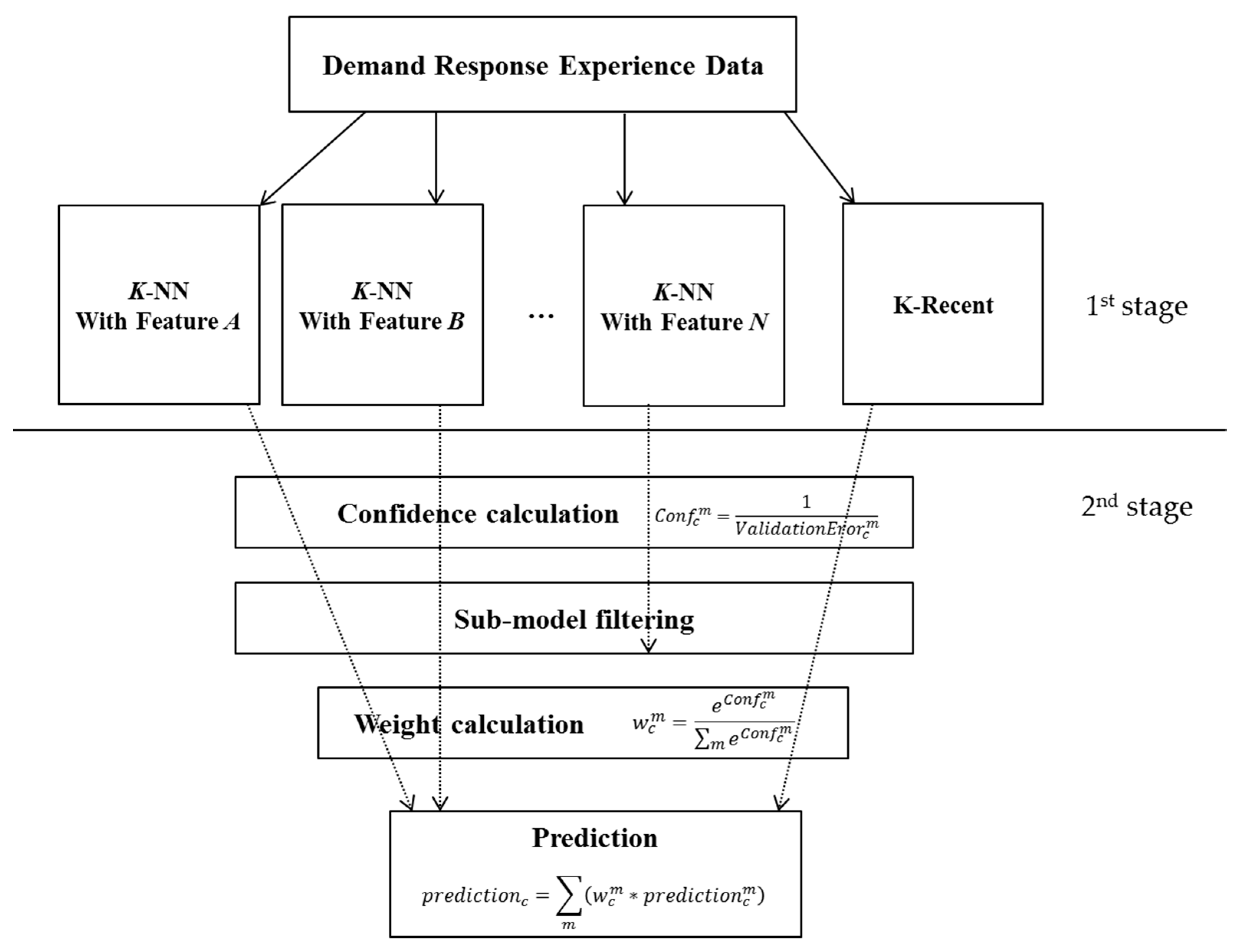
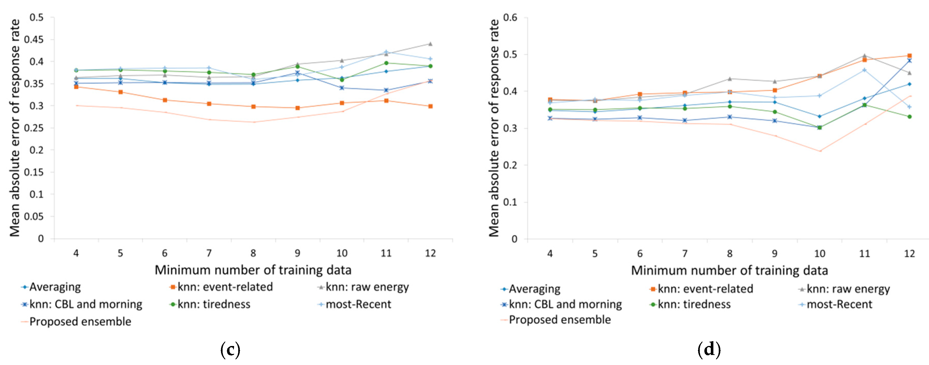
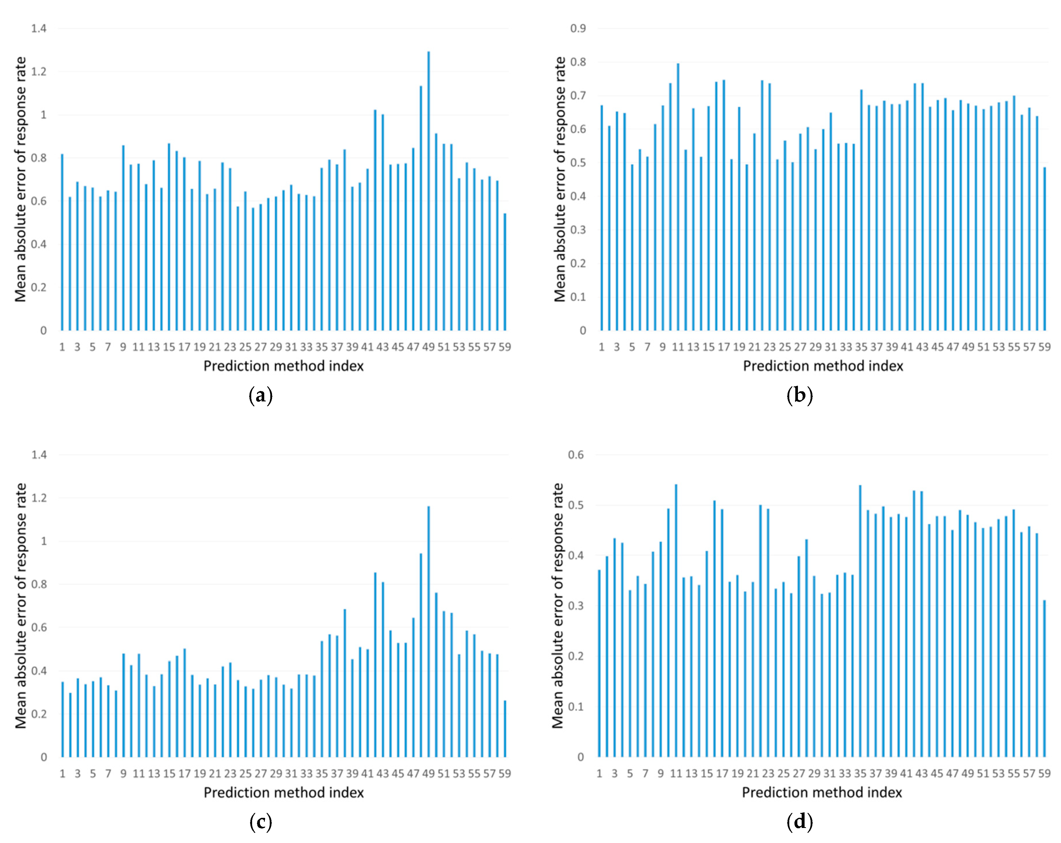
• Two difficulties, data sparsity and each customer’s individual characteristics, are alleviated with the proposed ensemble method. It is also verified that a single prediction algorithm cannot cover each customer’s unique response characteristics.
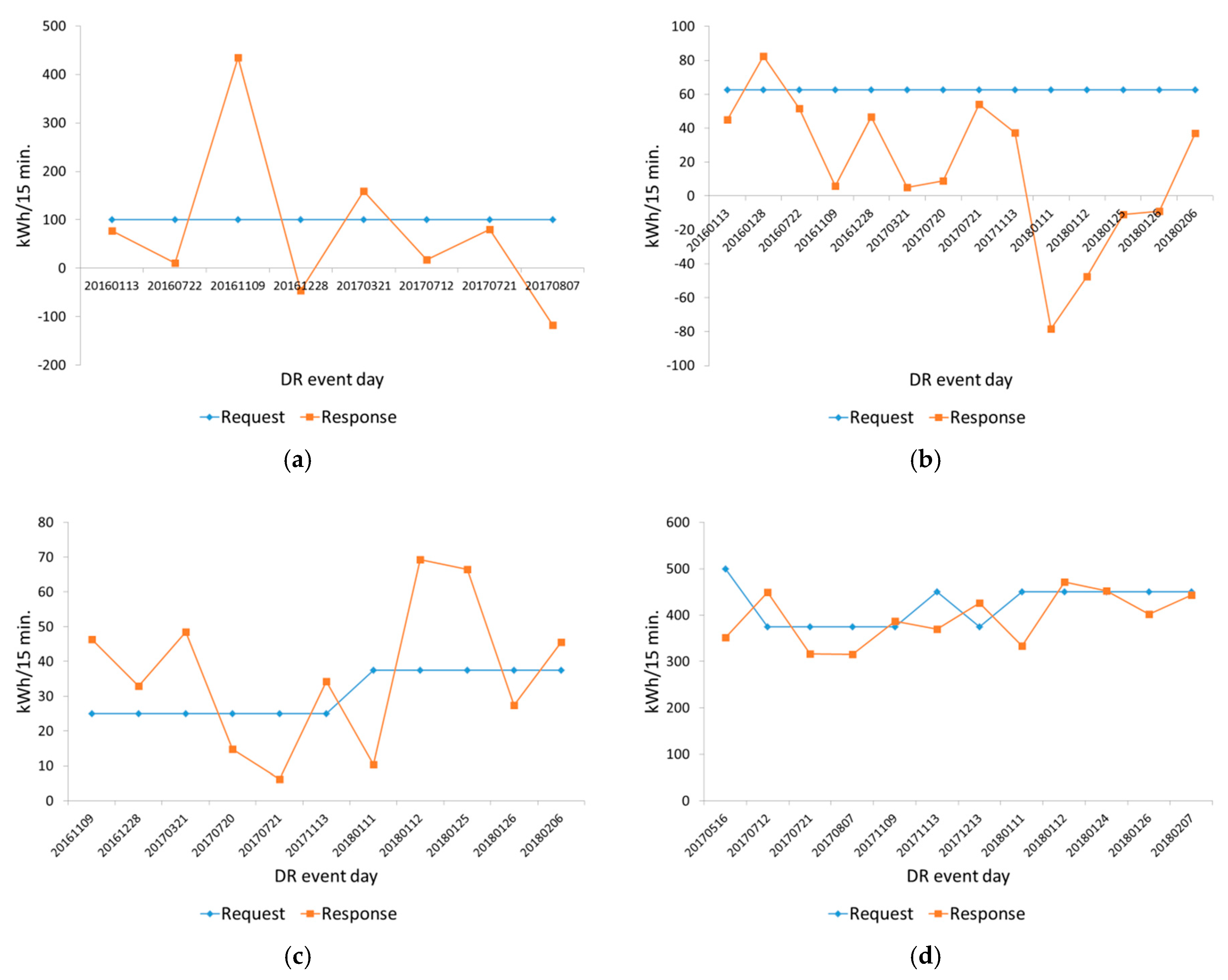
• In the experiment, the real data in a currently operating demand response system are used in order to increase the credibility. The proposed method provided an increased performance compared to other baseline methods with real data.

The rest of this paper is organized as follows. In Section 2, the details of the proposed prediction method are explained. In Section 3, the performance of the proposed method is compared to other baseline methods. Real load curtailment data from two demand response service providers are used in the experiment. The discussion resides in Section 4, and Section 5 concludes the paper.

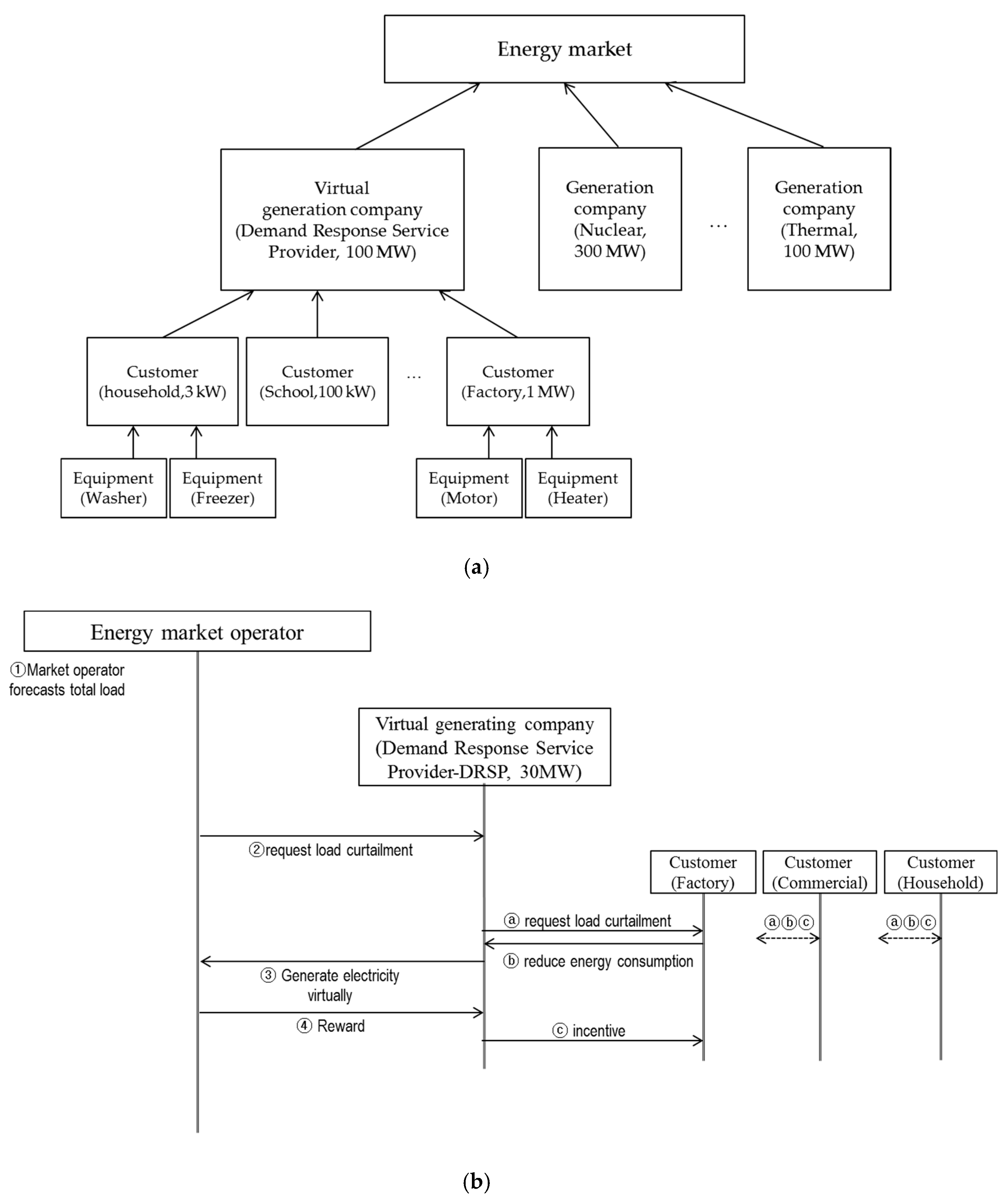
2. Proposed Prediction Model

2.1. Prediction Target

The goal of prediction is to estimate the amount of load curtailment in a DR event, as mentioned in the previous section. More specifically, the response rate, which is defined in Equation (1), is predicted. The reason we predict not the real load curtailment but the response rate is that different customers have different contracts and customers can even change contracts every year.

$$Response Rate=\frac{The amount of response \left(measured load reduction\right)}{The amount of request \left(requested load reduction\right)}$$

(1)

2.2. Prediction Model

The proposed prediction model uses an ensemble model based on the k-nearest neighbor method. Figure 3 presents the overall prediction framework, consisting of two stages.

In the first stage, the k-nearest neighbor method is basically used. The reason for this choice is that there is not enough data for each customer. Demand response itself is a rare event, activated only several times in a year. During a 30-month period, DR events were activated 15 times. This is too small a number for linear regression or neural network models. In the experiment, these methods provided poor performance. On the contrary, k-NN performed better because it needs only a few data points and the method is relatively free from overfitting. The features used in the prediction are described in

Table 1. Features used in the prediction.

Feature	Description
Raw energy consumption	Daily energy consumption pattern. It is the average of all normal days and consists of 96 dimensions.
Demand response (DR) event-related data	Information related to DR events. It consists of start time, duration, day of week, and day in year.
Customer baseline load	Customer baseline load in the DR event duration. For its calculation, refer to Section 3.1.
Tiredness	The index that presents the tiredness of a customer. Previous tiredness is divided by the interval between the latest DR event and the upcoming event day. If the interval is less than seven days, tiredness is increased. $Tirednes{s}_t=Tirednes{s}_{t-1}\ast \frac{7}{DR Interval}$
Morning energy consumption	The energy consumption in the morning (8:00~9:00 a.m.) of a DR event day.

. Raw energy consumption, event-time related features, tiredness, CBL, and morning usage are used as features. Weather data is not included in the proposed method because it does not provide an overall improvement in the experiment. In summary, in the proposed method, k-NN is conducted several times with these features and each k-NN with different input features constitutes a sub-model for the next stage. The k-recent method, which predicts the load curtailment to the average of the k most recent energy reduction, is also included in the sub-models. This is because recent experiences are more important than older ones. Other methods such as multi-layer perceptron (MLP), support vector regression (SVR), and convolutional neural network (CNN) were included in the sub-models in the first place. However, they are removed from final proposal because they do not provide performance improvement, as briefly mentioned in Section 1. As a result, five k-NN sub-models and one k-recent sub-model are implemented in the proposed method.

In the second stage, the ensemble is performed to improve the performance. Basically, the final prediction is calculated as the weighted sum of the sub-model predictions at the end of the stage. To calculate weights, the validation errors of sub-models are first calculated according to Equation (2) and the confidences of sub-models are calculated as in Equation (3). The inverse of the average prediction error is defined as the confidence of the sub-model prediction.

$$ValidationErro{r}_c^m=\frac{{{\displaystyle \sum }}_d(Pr{e}_c^{d,m}-L{C}_c^{d,m})}{N}$$

(2)

$$Con{f}_c^m=\frac{1}{ValidationEro{r}_c^m}$$

(3)

where c is the customer, d is the validation day, m is the sub-model type; $Con{f}_c^m$ is the confidence of sub-model m for customer c, $Pr{e}_c^{d,m}$ is the predicted energy reduction of sub-model m for customer c on day d, $L{C}_c^{d,m}$ is the real load curtailment of sub-model m for customer c on day d, and N is the number of days in validation set D.

The validation error of a sub-model is calculated based on the validation set. N preceding DR event days are used as the validation set and the prediction error on these validation days are averaged to produce ValidationError. We fixed the number of validation days to be the most recent four days. Figure 4 presents the concept of the training set, validation set, and test set. In Figure 4, the validation error of a sub-model is the average of the prediction error from V1 through V4 using that sub-model.

Before the final prediction, a sub-model filtering step is inserted. In this step, those methods that provide higher confidence than the averaging method are only chosen for further processing. In the averaging method, the response is predicted as the average of the past DR event days’ responses. If the confidence of a sub-model is worse than that of the averaging method, it is certain that the inclusion of that method degrades the performance. After the filtering stage, the surviving sub-models’ confidences are passed through SOFTMAX function, as in Equation (4), and the final prediction is calculated as the weighted sum of survived sub-model predictions, as in Equation (5).

$$w_c^m=\frac{e^{Con{f}_c^m}}{{{\displaystyle \sum }}_m{e}^{Con{f}_c^m}}$$

(4)

$$predictio{n}_c={\displaystyle \sum }_m\left(w_c^m\ast predictio{n}_c^m\right)$$

(5)

This second stage enables the proposed method to find the unique characteristics of each customer and build a different model for each customer. A customer who mostly relies on tiredness and a customer who significantly depends on the event starting time will have different confidences for each sub-model, so that the final prediction model will be unique for each customer. Other meta-ensembles such as stacked generalization [36] are not included in the proposed second stage because the data size is too small to apply another complicated algorithm in the second stage.

The prediction of a customer’s response is conducted using that customer’s own data. Although there is large number of customers in the data set, other customers’ data are not used because each customer has its own characteristics. In the experiment, however, the result with one unified data set is also compared with the proposed model.

3. Experiment

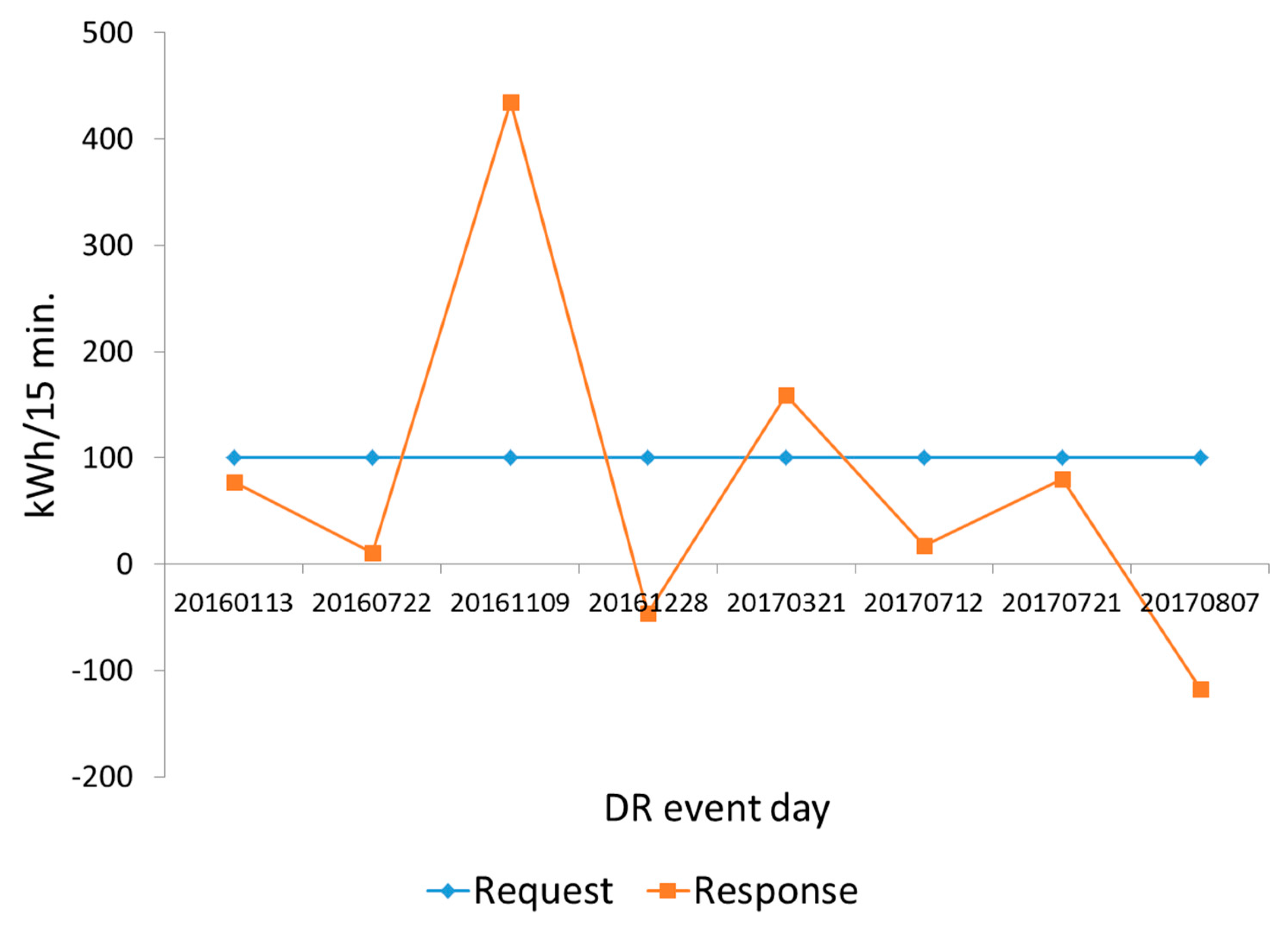
3.1. Data Description

Real demand response data from two service providers are used in the experiments. The two data sets are not merged but are experimented separately because the specific data are the assets of each service provider. These two data sets consist of 64 customers and 196 customers, respectively. Data from 1 January 2016 to 28 February 2018 are used. During this period, DR requests were activated a total of 15 times. However, this does not mean that every customer received 15 requests. This is because customers are clustered to a few groups and DR activation was conducted based on these subgroups. In the experiments, only DR event days with five or more preceding DR event days are included in the test set. The test is based on each event day and on each customer, yielding the totals of tested days of 440 and 761, respectively.

The calculation of the amount of load curtailment requires the estimation of the customer baseline load (CBL). The CBL is the expected energy consumption in the case of no DR event. In the experiment, five preceding normal days are selected and one day that shows minimum energy consumption is eliminated. The customer baseline load is calculated as an average of the resulting four days, as stated in the market procedure [5].

3.2. Experiment Result

First, real load reduction histories from several real customers are presented to show the characteristics of customers. In Figure 5, it is shown that Customer #1, #2, and #3 provided very unstable responses day by day. Customers #1 and # 2 even provided energy reduction values that are less than zero, meaning that they increased energy consumption on some days. In particular, Customer #2 provided enough load curtailment only one time out of 14 requests. Customer #3 provided six successes out of 11 trials. Customer #4 provided a relatively stable response compared to the other three customers. From these data, it is clear that the characteristics of each customer are different from those of others. The goal of this paper is to predict the amount of energy reduction on a given day, in these uncertain circumstances.

From Figure 6, Figure 7 and Figure 8, the performance of the proposed method is presented in terms of the mean absolute error (MAE) of all customers. In Figure 6, minimum number of required training data is varied. This means that the test is conducted only if the amount of training data is greater than this number. If the minimum number is too small, the prediction will be inaccurate because the training set is not enough. If it is too large, the size of the test data set will be too small to achieve an accurate result. As it can be clearly seen in Figure 6a,b the MAE of the proposed method shows a decreased prediction error compared to sub-models’ individual result. The most-recent method predicts the load curtailment according to the most recent DR event day.

The error values are quite large in Figure 6a,b because there are some outlier customers that provide exceptionally high responses. For example, one customer exceptionally reduced energy on a given day, up to fifteen times its contracted amount. Such responses can severely distort the performance graph because they greatly affect the average error. In Figure 6c,d these exceptional outliers are eliminated and the number of tested days is decreased to 334 and 650, respectively, for the two service providers. It should be noted that when the minimum amount of training data is too large, the number of tested days is so small that an unstable result is obtained. However, apart from this, the performance of the proposed method provides a much more stable and improved result in both data sets, confirming that the ensemble method is suitable. This means that the weights in the ensemble automatically reflect the characteristics of each customer.

Usually, it is essential to compare the proposed method to up-to-date prediction methods in this field. However, as mentioned in Section 1, this research area is quite new and the baselines that we can consider are limited. Although there are related researches [11,12], as mentioned in the Introduction Section, it is not easy to implement those methods because their descriptions are not adequate and the target customers are different from those of our system. Their targets are university campus buildings, while ours are various demand response customers including factories, shopping centers, and even a fish farm, located across a nation. Instead, we compared our method to various well-known machine learning methods such as linear regression, neural network, support vector machine, and even convolutional neural network to assess the performance of the proposed method. This comparison is presented in Figure 7.

In this experiment, the minimum number of training data points is set to eight, which is considered to be reasonable training data set size and test set size. The compared methods include averaging (index 1), k-NN (from indices 2 to 8), linear regression (from indices 9 to 14), multi-layer perceptron (from indices 15 to 20), support vector regression (from indices 21 to 26), k-recent (from indices 27 to 31), and convolutional neural network (from indices 32 to 34). In each method, the input features described in Table 1 are separately used in each index. k is varied in the k-recent method and convolutional networks which consist of three convolution layers with RELU functions [37] are tested. k-NN with weather data as an input feature is also tested in index 8. Other hyper-parameters in basic models are set to default values in Weka [38]. The first half (from indices 1 to 34) of the compared methods does not use other customers’ data; that is, each customer’s model is trained with his own demand response history data. The second half (from indices 35 to 58) uses other customers’ data, as well. This means that the model is trained using all of the historical data from various customers, because the inclusion of other customers’ data dramatically increases the total number of training data points. Because the energy consumption level of each customer is different, the daily energy consumption pattern is normalized to its maximum value. Finally, the proposed method is indexed to 59 at the end of the bar chart. Although there were other unpresented experiments with other parameter settings, the best result of each method is presented.

In the results, first, it is observed that other customers’ data do not improve the prediction performance. Although data sparsity forced us to use the other customers’ response data, their inclusion (right half of graphs) only increased the prediction error. Second, prebuilt models such as linear regression or neural network (indices 9 to 20) do not provide a good performance due to the data sparsity, as mentioned earlier. Third, weather data (index 8) is not beneficial because, in many cases, the main source of energy reduction is not from HVAC (heating, ventilation, and air conditioning), in many cases. Finally, the proposed ensemble method outperformed the other various methods regardless of outlier inclusion or exclusion in both data sets. For example, in the case of outlier exclusion, the proposed method produced MAEs of 0.26 and 0.31 in the two data sets, respectively, compared to the results of 0.35 and 0.37 achieved using averaging method.

Because a DRSP needs to add the load curtailment of a given customer on a DR event day, it is necessary to monitor its performance on a daily basis. Figure 8 compares the average prediction error of each DR event day. As shown in Figure 8, the proposed method provides a decreased error for most DR event days, as compared to the other baselines in both data sets. In Figure 8b, on 20 December 2017, the most-recent method provided exceptionally high prediction error, up to 10. Because this exceptional number makes the performance on other days undistinguishable, the maximum of y-axis was set to 4 in order to observe the performance at a glance. At the right side of figure, indicating more training data, it is clear that the prediction error is decreased in the proposed method. Figure 8a,b confirm that the proposed method can actually be used in a real demand system that operates on a daily basis.

4. Discussion

According to our experiment, there are a few points that can be mentioned. First, the prediction of load curtailment is possible, despite the two difficulties of data sparsity and the different characteristics of customers. Although these issues seem to make the prediction more difficult to calculate, the performance can be improved compared to other baseline approaches.

Second, the prediction is not an easy task in general. The MAEs of the response rate achieved using the proposed method without outlier elimination are 0.49 and 0.54 in the two data sets, respectively. These numbers are too large. Although they are decreased to 0.26 and 0.31 with some outlier elimination, they are still large numbers—indicating that the prediction still needs to be improved.

Third, it was found that other customers’ data do not help the prediction at all. At the beginning of this research, it seemed that other customers’ data could be an attractive asset because the data are so sparse in this application. It is, however, certain that other customers’ data do not improve the prediction performance, as the characteristics of each customer are so different.

Fourth, an important customer for a DRSP might require a special training. Important customers who have large contracts or provide very unstable load curtailments can be trained by an exceptional individual model because they may affect sum of load curtailment otherwise. Current DRSPs already manage the list of such important customers. In other words, the responses of all customers can be predicted using the proposed method, and a few important customers can be further investigated to improve the prediction performance even more.

Finally, the prediction performance can be improved as time passes. In Figure 8, the performance shows a stable result at the right side of the figure, where more data is employed in the data set. As demand response experience data accumulate, it is certain that the prediction accuracy will improve.

5. Conclusions

The amount of load curtailment in demand response is neither predetermined nor reliable, as proved in this paper—especially in the liberalized energy market. In this circumstance, a virtual generation company that is composed of many demand response customers cannot provide stable energy consumption reduction. As a result, the prediction of demand response should be considered seriously.

In this paper, the amount of load curtailment was predicted for each demand response customer based on past data. Although the sparsity of data and the unique characteristics of each customer make the problem difficult, the proposed ensemble method based on k-NN alleviated these problems and provided the best prediction performance (down to 0.26 and 0.31 for the two data sets, respectively) as compared with other many baselines, such as multi-layer perceptron and support vector regression. The daily MAEs of the response rate in the proposed method were also decreased compared to those of the baseline methods.

In the future, the optimization of demand response will be conducted based on the prediction of each customer’s response. If a DRSP can know each customer’s future load curtailment, participating customers in a DR event can be selected by the DRSP so as to avoid wasting resources and avoid receiving a penalty. Additionally, the prediction method can be applied to other energy applications such as distributed energy resources, as it is highly likely that they also are characterized by a small amount of data and different characteristics for each resource. In summary, the proposed method can be used as one of several prediction blocks in energy optimization systems.

References

1. US Department of Energy. Benefits of Demand Response in Electricity Markets and Recommendations for Achieving Them; US Department of Energy: Washington, DC, USA, 2006.
2. Agency, I.E. The Power to Choose: Demand Response in Liberalised Electricity Markets; OECD Publishing: Paris, France, 2003. [Google Scholar]
3. Albadi, M.H.; El-Saadany, E.F. A summary of demand response in electricity markets. Electr. Power Syst. Res. 2008, 78, 1989–1996. [Google Scholar] [CrossRef]
4. Kang, J.; Lee, J.-H. Data-Driven Optimization of Incentive-based Demand Response System with Uncertain Responses of Customers. Energies 2017, 10, 1537. [Google Scholar] [CrossRef]
5. Korea Energy Market Operation Protocol. Available online: http://www.kpx.or.kr (accessed on 18 September 2017). (In Korean).
6. Atkinson, S.E. Responsiveness to time-of-day electricity pricing: First empirical results. J. Econom. 1979, 9, 79–95. [Google Scholar] [CrossRef]
7. Herter, K. Residential implementation of critical-peak pricing of electricity. Energy Policy 2007, 35, 2121–2130. [Google Scholar] [CrossRef] [Green Version]
8. Taylor, T.N.; Schwarz, P.M.; Cochell, J.E. 24/7 hourly response to electricity real-time pricing with up to eight summers of experience. J. Regul. Econ. 2005, 27, 235–262. [Google Scholar] [CrossRef]
9. Ghazvini, M.A.F.; Faria, P.; Ramos, S.; Morais, H.; Vale, Z. Incentive-based demand response programs designed by asset-light retail electricity providers for the day-ahead market. Energy 2015, 82, 786–799. [Google Scholar] [CrossRef]
10. Aman, S.; Frincu, M.; Chelmis, C.; Noor, M.; Simmhan, Y.; Prasanna, V.K. Prediction models for dynamic demand response: Requirements, challenges, and insights. In Proceedings of the 2015 IEEE International Conference on Smart Grid Communications (SmartGridComm), Miami, FL, USA, 2–5 November 2015; pp. 338–343. [Google Scholar]
11. Chelmis, C.; Aman, S.; Saeed, M.R.; Frincu, M.; Prasanna, V.K. Estimating Reduced Consumption for Dynamic Demand Response. In Proceedings of the AAAI Workshop on Computational Sustainability, Austin, TX, USA, 25–26 January 2015. [Google Scholar]
12. Aman, S.; Chelmis, C.; Prasanna, V.K. Learning to REDUCE: A Reduced Electricity Consumption Prediction Ensemble. In Proceedings of the AAAI Workshop: AI for Smart Grids and Smart Buildings, Phoenix, AZ, USA, 12–13 February 2016. [Google Scholar]
13. Ninagawa, C.; Kondo, S.; Morikawa, J. Prediction of aggregated power curtailment of smart grid demand response of a large number of building air-conditioners. In Proceedings of the 2016 International Conference on Industrial Informatics and Computer Systems (CIICS), Sharjah, UAE, 13–16 March 2016; pp. 1–4. [Google Scholar]
14. Barakat, E.H.; Al-Qassim, J.M.; Al Rashed, S.A. New model for peak demand forecasting applied to highly complex load characteristics of a fast developing area. IEE Proc. C Gener. Transm. Distrib. 1992, 139, 136–140. [Google Scholar] [CrossRef]
15. Fan, J.Y.; McDonald, J.D. A real-time implementation of short-term load forecasting for distribution power systems. IEEE Trans. Power Syst. 1994, 9, 988–994. [Google Scholar] [CrossRef]
16. Chen, J.-F.; Wang, W.-M.; Huang, C.-M. Analysis of an adaptive time-series autoregressive moving-average (ARMA) model for short-term load forecasting. Electr. Power Syst. Res. 1995, 34, 187–196. [Google Scholar] [CrossRef]
17. Huang, S.R. Short-term load forecasting using threshold autoregressive models. IEE Proc. C Gener. Transm. Distrib. 1997, 144, 477–481. [Google Scholar] [CrossRef]
18. Moghram, I.; Rahman, S. Analysis and evaluation of five short-term load forecasting techniques. IEEE Trans. Power Syst. 1989, 4, 1484–1491. [Google Scholar] [CrossRef]
19. Hyde, O.; Hodnett, P.F. An adaptable automated procedure for short-term electricity load forecasting. IEEE Trans. Power Syst. 1997, 12, 84–94. [Google Scholar] [CrossRef]
20. Al-Garni, A.Z.; Zubair, S.M.; Nizami, J.S. A regression model for electric-energy-consumption forecasting in Eastern Saudi Arabia. Energy 1994, 19, 1043–1049. [Google Scholar] [CrossRef]
21. Infield, D.G.; Hill, D.C. Optimal smoothing for trend removal in short term electricity demand forecasting. IEEE Trans. Power Syst. 1998, 13, 1115–1120. [Google Scholar] [CrossRef]
22. Djukanovic, M.; Babic, B.; Sobajic, D.J.; Pao, Y.-H. Unsupervised/supervised learning concept for 24-hour load forecasting. IEE Proc. C Gener. Transm. Distrib. 1993, 140, 311–318. [Google Scholar] [CrossRef]
23. Beccali, M.; Cellura, M.; Brano, V.L.; Marvuglia, A. Forecasting daily urban electric load profiles using artificial neural networks. Energy Convers. Manag. 2004, 45, 2879–2900. [Google Scholar] [CrossRef]
24. Kim, K.-H.; Park, J.-K.; Hwang, K.-J.; Kim, S.-H. Implementation of hybrid short-term load forecasting system using artificial neural networks and fuzzy expert systems. IEEE Trans. Power Syst. 1995, 10, 1534–1539. [Google Scholar]
25. Brown, R.E.; Hanson, A.P.; Hagan, D.L. Long range spatial load forecasting using non-uniform areas. In Proceedings of the 1999 IEEE Transmission and Distribution Conference, New Orleans, LA, USA, 11–16 April 1999; Volume 1, pp. 369–373. [Google Scholar]
26. Mori, H.; Kobayashi, H. Optimal fuzzy inference for short-term load forecasting. In Proceedings of the 1995 IEEE Power Industry Computer Application Conference, Salt Lake City, UT, USA, 7–12 May 1995; pp. 312–318. [Google Scholar]
27. Raza, M.Q.; Khosravi, A. A review on artificial intelligence based load demand forecasting techniques for smart grid and buildings. Renew. Sustain. Energy Rev. 2015, 50, 1352–1372. [Google Scholar] [CrossRef]
28. Khan, A.R.; Mahmood, A.; Safdar, A.; Khan, Z.A.; Khan, N.A. Load forecasting, dynamic pricing and DSM in smart grid: A review. Renew. Sustain. Energy Rev. 2016, 54, 1311–1322. [Google Scholar] [CrossRef]
29. Chao, H. Demand response in wholesale electricity markets: The choice of customer baseline. J. Regul. Econ. 2011, 39, 68–88. [Google Scholar] [CrossRef]
30. Mathieu, J.L.; Callaway, D.S.; Kiliccote, S. Variability in automated responses of commercial buildings and industrial facilities to dynamic electricity prices. Energy Build. 2011, 43, 3322–3330. [Google Scholar] [CrossRef] [Green Version]
31. Coughlin, K.; Piette, M.A.; Goldman, C.; Kiliccote, S. Statistical analysis of baseline load models for non-residential buildings. Energy Build. 2009, 41, 374–381. [Google Scholar] [CrossRef] [Green Version]
32. Chelmis, C.; Aman, S.; Saeed, M.R.; Frincu, M.; Prasanna, V.K. Predicting reduced electricity consumption during dynamic demand response. In Proceedings of the AAAI Workshop on Computational Sustainability, Austin, TX, USA, 25–26 January 2015. [Google Scholar]
33. Ziekow, H.; Goebel, C.; Struker, J.; Jacobsen, H.-A. The potential of smart home sensors in forecasting household electricity demand. In Proceedings of the 2013 IEEE International Conference on Smart Grid Communications (SmartGridComm), Vancouver, BC, Canada, 21–24 October 2013; pp. 229–234. [Google Scholar]
34. Altman, N.S. An introduction to kernel and nearest-neighbor nonparametric regression. Am. Stat. 1992, 46, 175–185. [Google Scholar]
35. Krizhevsky, A.; Sutskever, I.; Hinton, G.E. Imagenet classification with deep convolutional neural networks. In Proceedings of the Advances in Neural Information Processing Systems, Lake Tahoe, NV, USA, 3–8 December 2012; pp. 1097–1105. [Google Scholar]
36. Wolpert, D.H. Stacked generalization. Neural Netw. 1992, 5, 241–259. [Google Scholar] [CrossRef] [Green Version]
37. Glorot, X.; Bordes, A.; Bengio, Y. Deep sparse rectifier neural networks. In Proceedings of the Fourteenth International Conference on Artificial Intelligence and Statistics, Ft. Lauderdale, FL, USA, 11–13 April 2011; pp. 315–323. [Google Scholar]
38. Weka 3—Data Mining with Open Source Machine Learning Software in Java. Available online: https://www.cs.waikato.ac.nz/ml/weka/ (accessed on 27 August 2018).
Figure 1. The structure of the considered demand response system. (a) Overall market structure; (b) detailed transaction procedure; Adapted with permission from [4], Jimyung Kang and Jee-Hyong Lee, Energies, MDPI, 2017. DRSP: demand response service provider.
Energies 11 02905 g001
Figure 2. Uncertainty of load curtailment.
Energies 11 02905 g002
Figure 3. The proposed prediction model.
Energies 11 02905 g003
Figure 4. Training, validation, and test set structure.
Energies 11 02905 g004
Figure 5. The amount of load reduction from several customers. (a) Customer #1; (b) Customer #2; (c) Customer #3; (d) Customer #4.
Energies 11 02905 g005
Figure 6. Prediction error comparison. (a) Customer set A (From service provider A); (b) Customer set B (From service provider B); (c) Customer set A (Outliers eliminated); (d) Customer set B (Outliers eliminated).
Energies 11 02905 g006aEnergies 11 02905 g006b
Figure 7. Prediction error comparison with other various methods. (Index 1: averaging; index 59: the proposed method). (a) Customer set A (From service provider A); (b) Customer set B (From service provider B); (c) Customer set A (Outliers eliminated); (d) Customer set B (Outliers eliminated).
Energies 11 02905 g007
Figure 8. Prediction error comparison for each DR event day. (a) Customer set A (From service provider A); (b) Customer set B (From service provider B).
Energies 11 02905 g008