A Review and New Problems Discovery of Four Simple Decentralized Maximum Power Point Tracking Algorithms—Perturb and Observe, Incremental Conductance, Golden Section Search, and Newton’s Quadratic Interpolation


Abstract
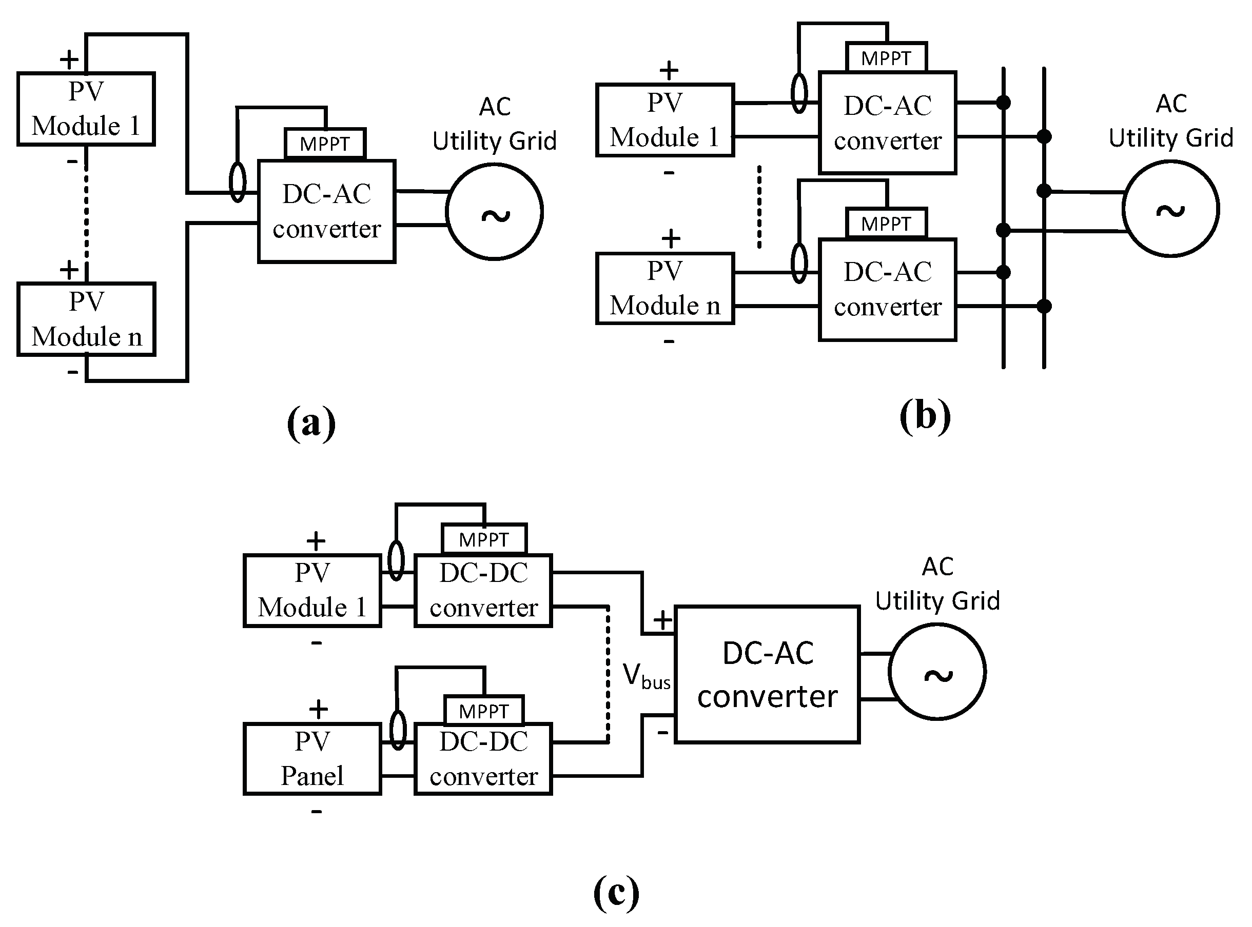
:1. Introduction
2. Review of Various Methodologies
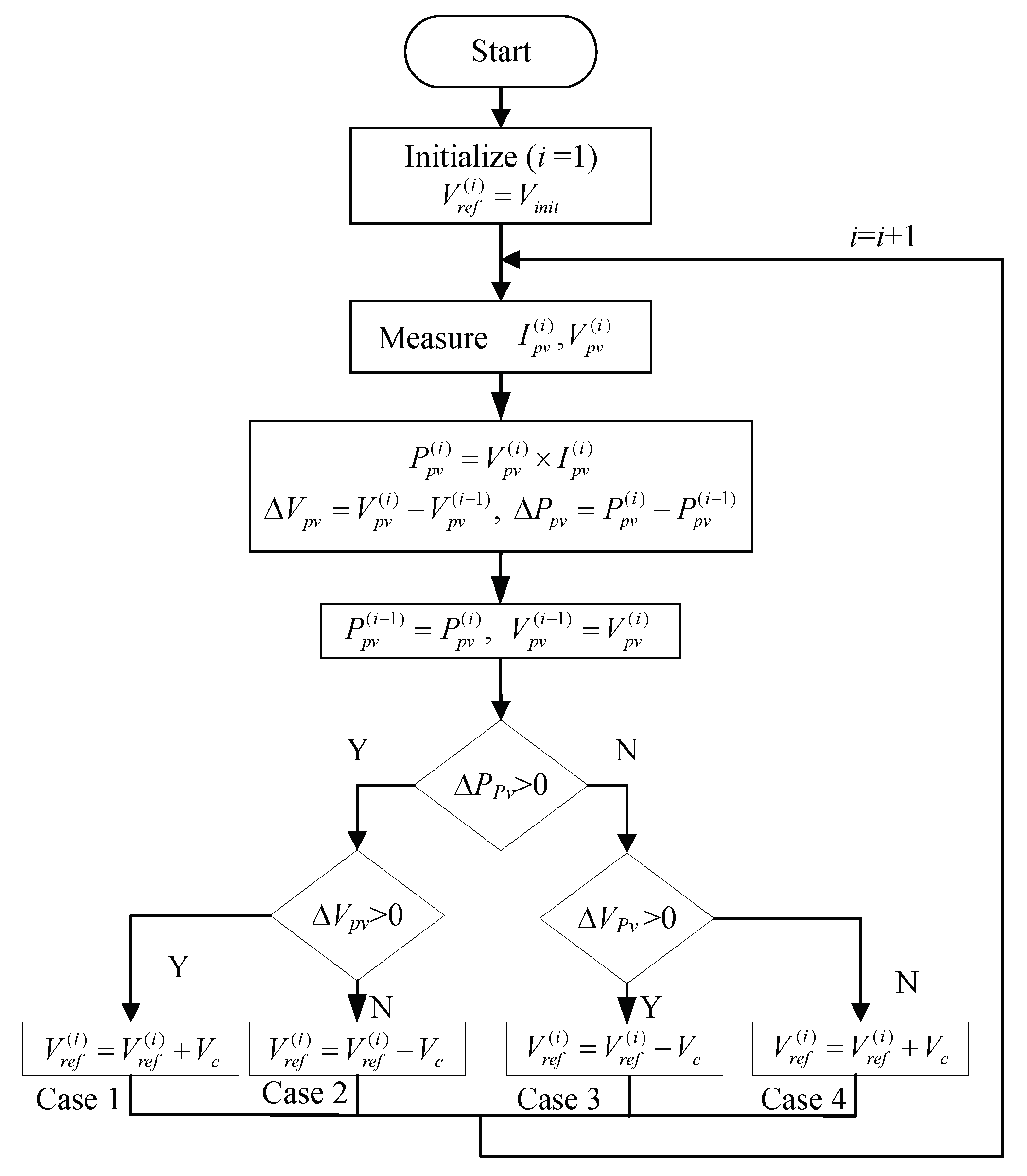
2.1. Perturb-and-Observe ()
2.2. Incremental Conductance
- when , the operating point is to the right of the MPP;
- when , the operating point is at the MPP;
- when , the operating point is to the left of the MPP.
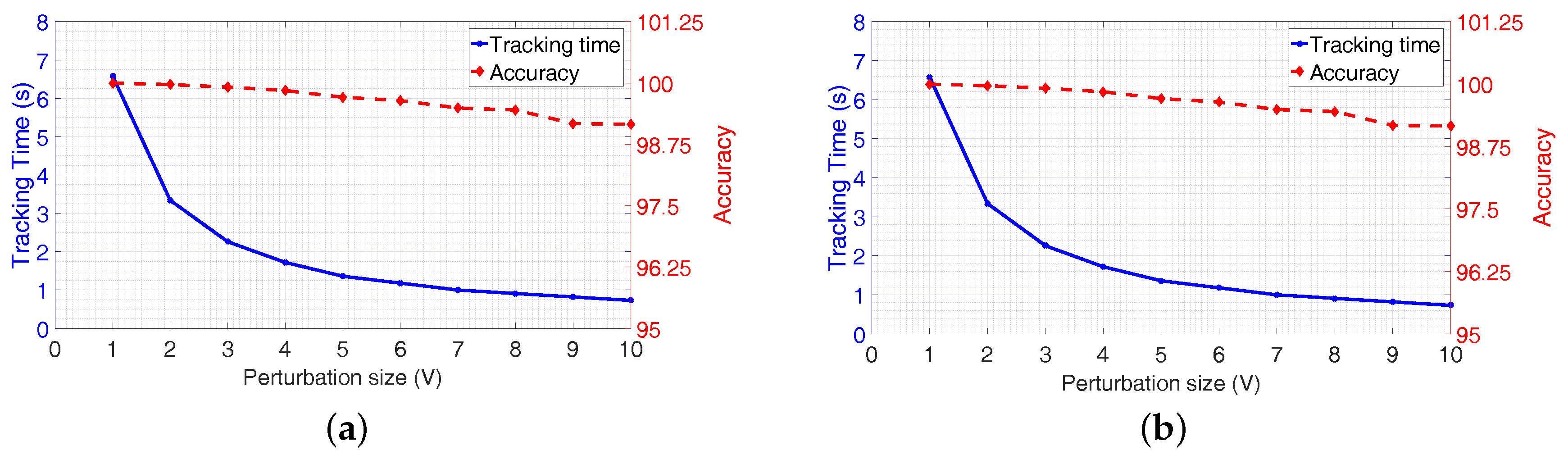
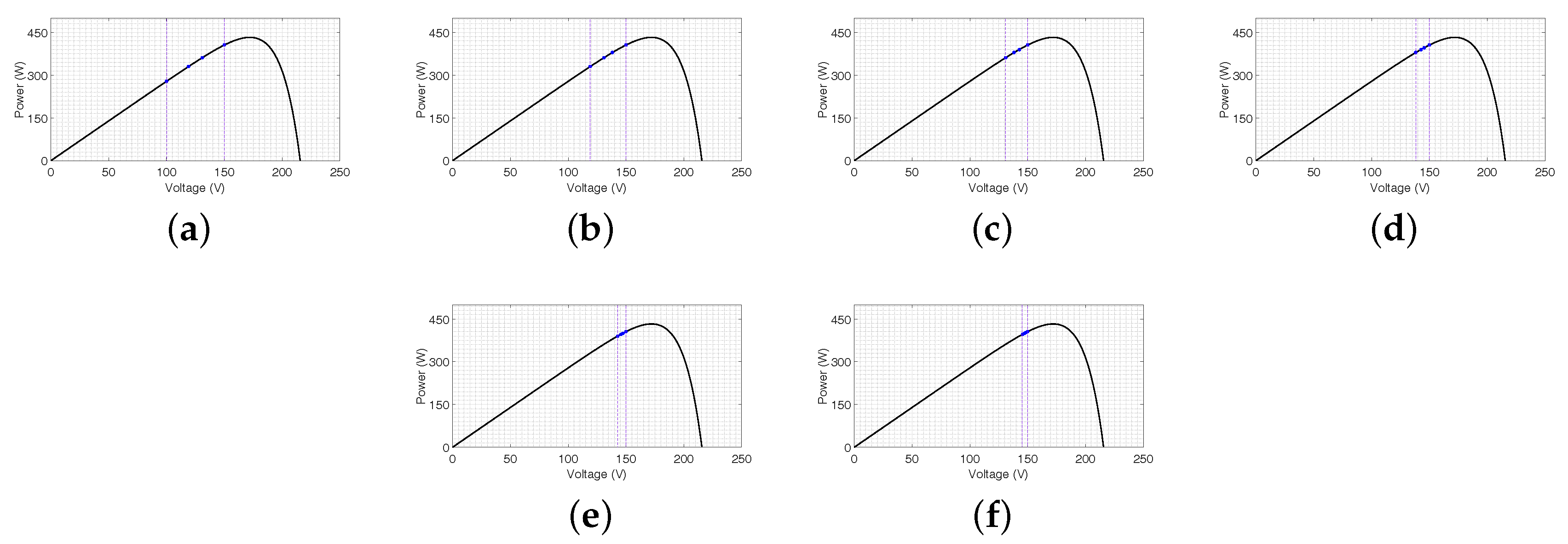
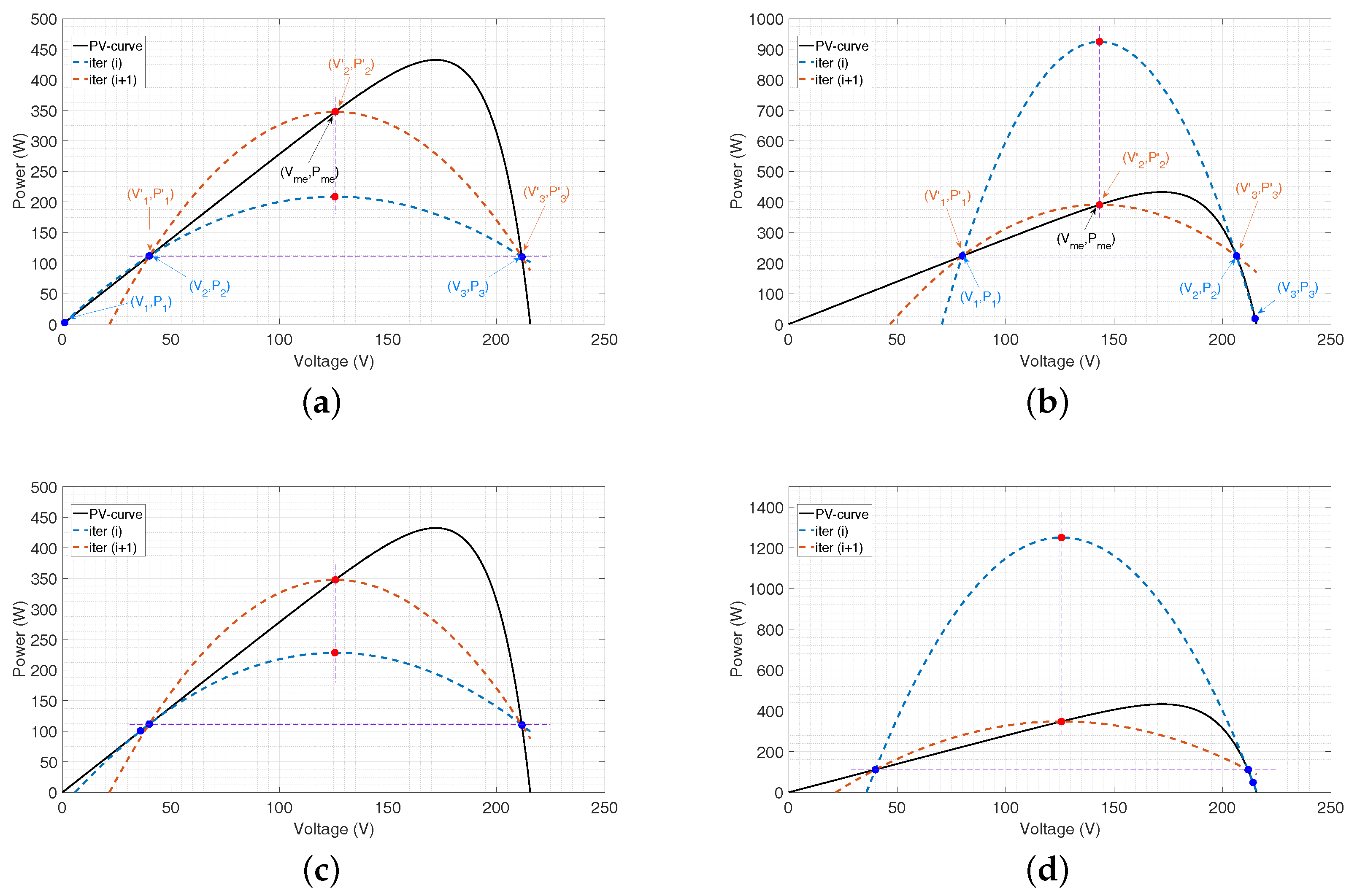
2.3. Golden Section Search
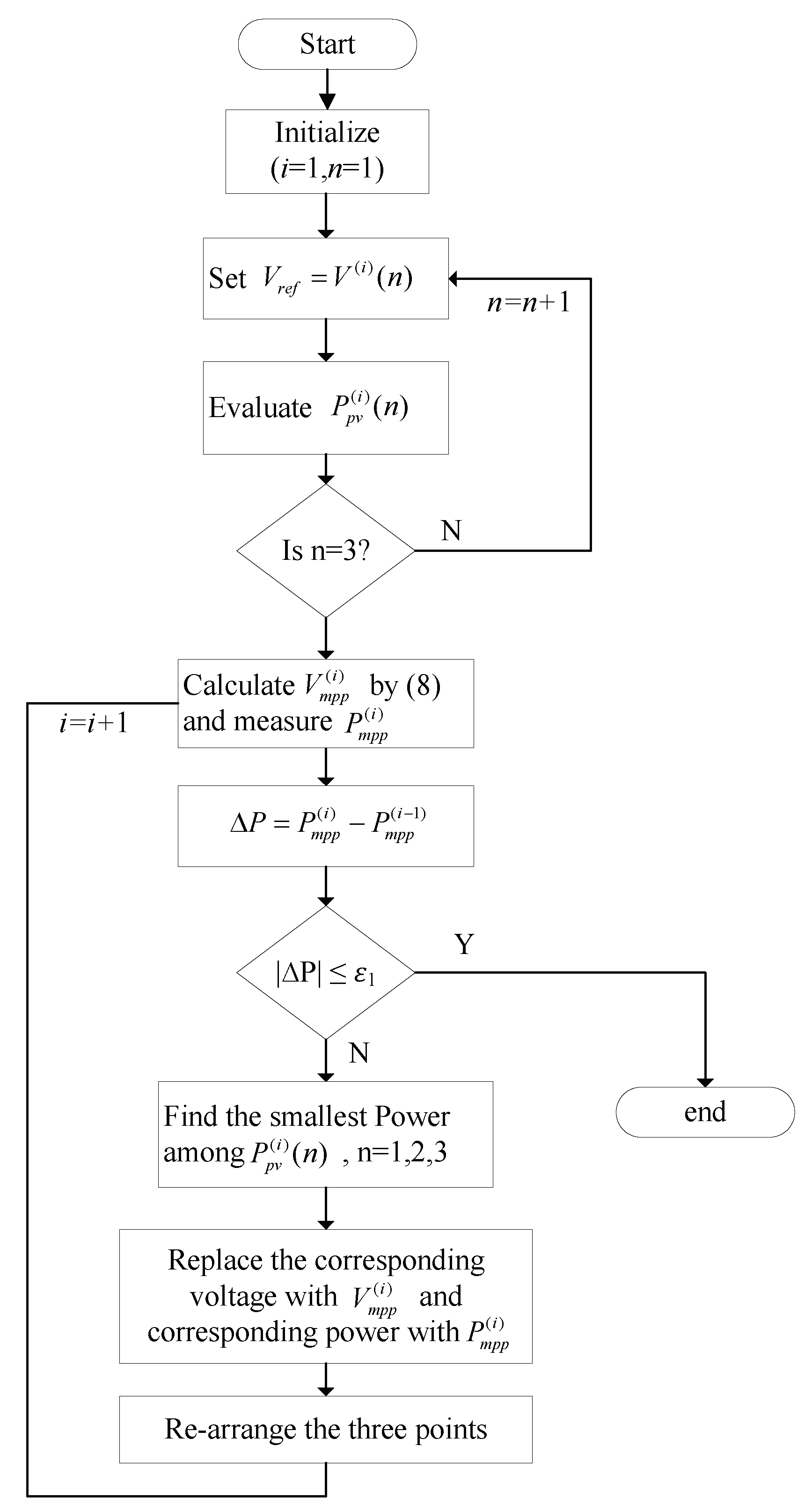
2.4. Newton Quadratic Interpolation
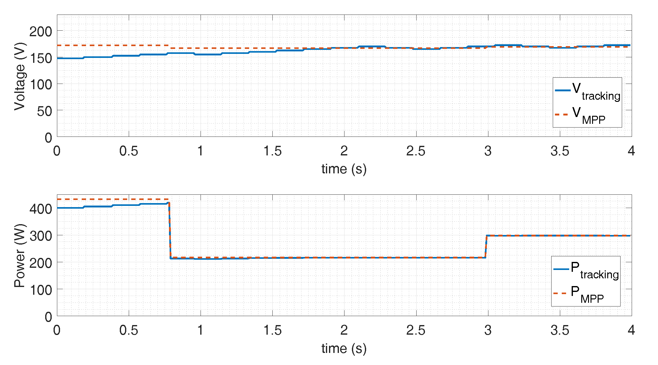
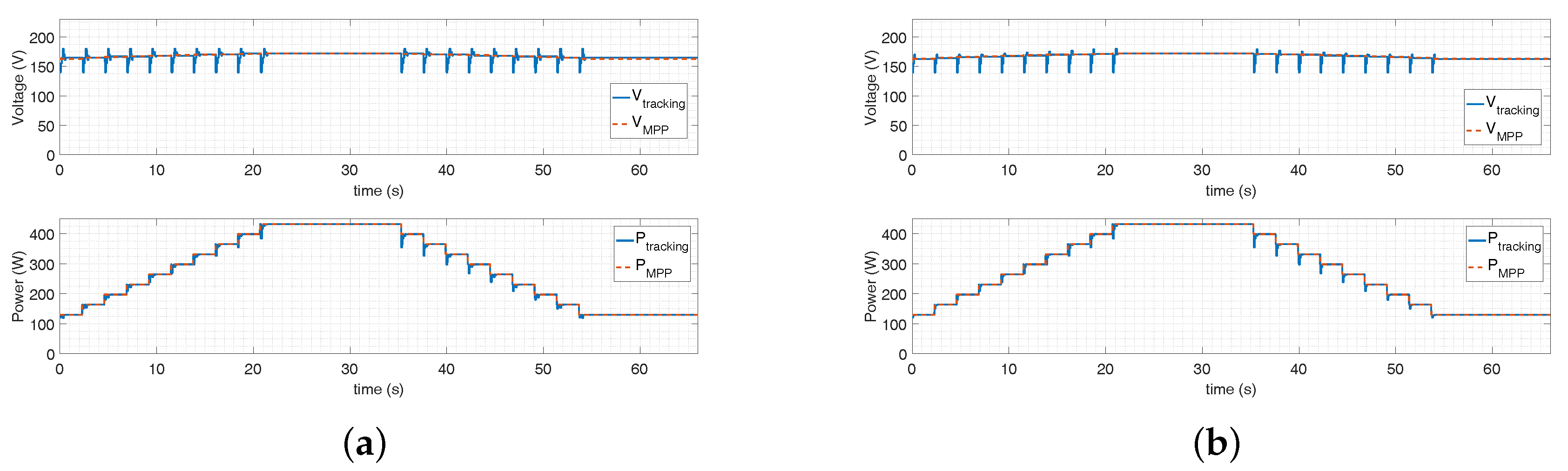
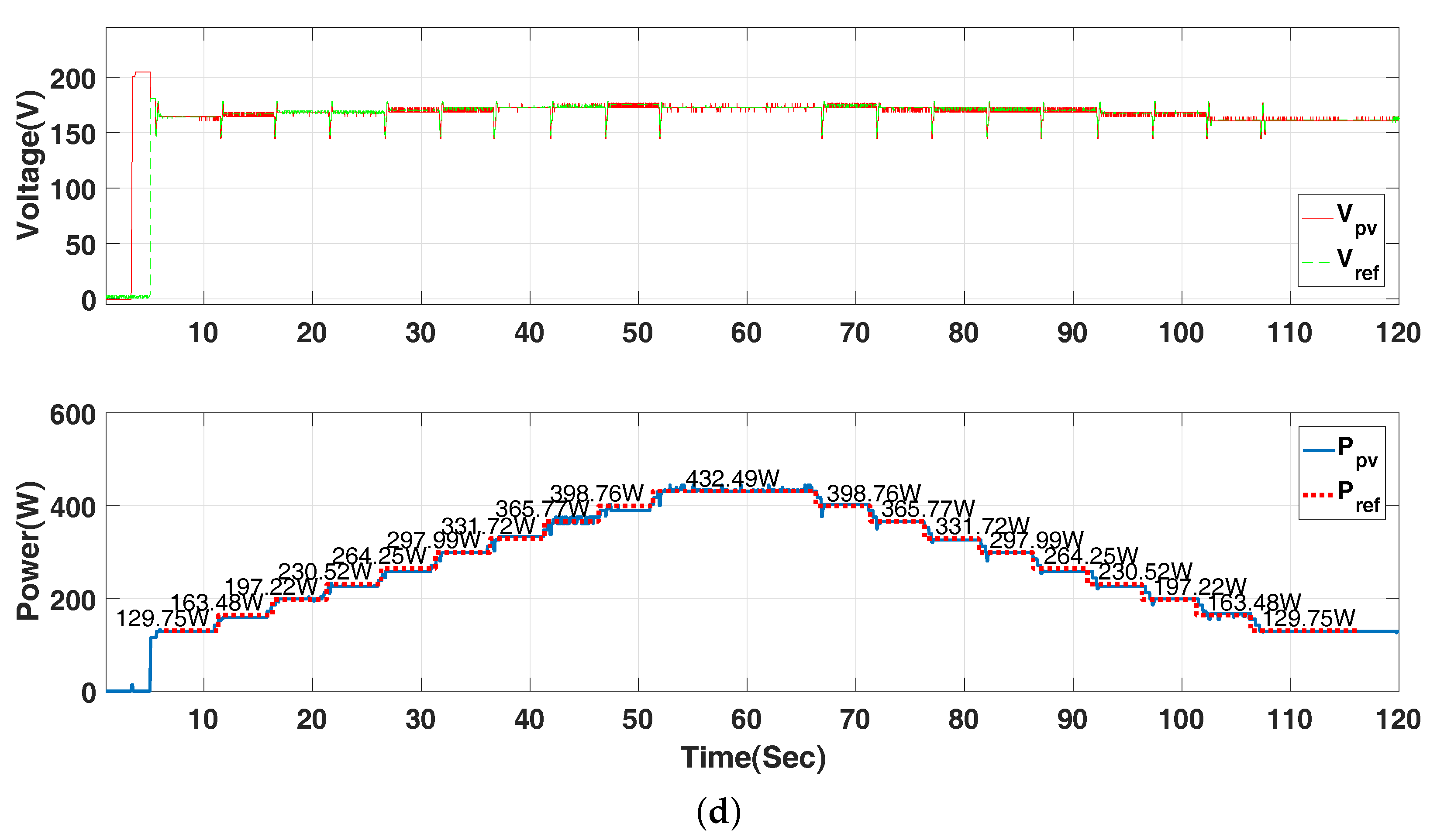
3. Discussion
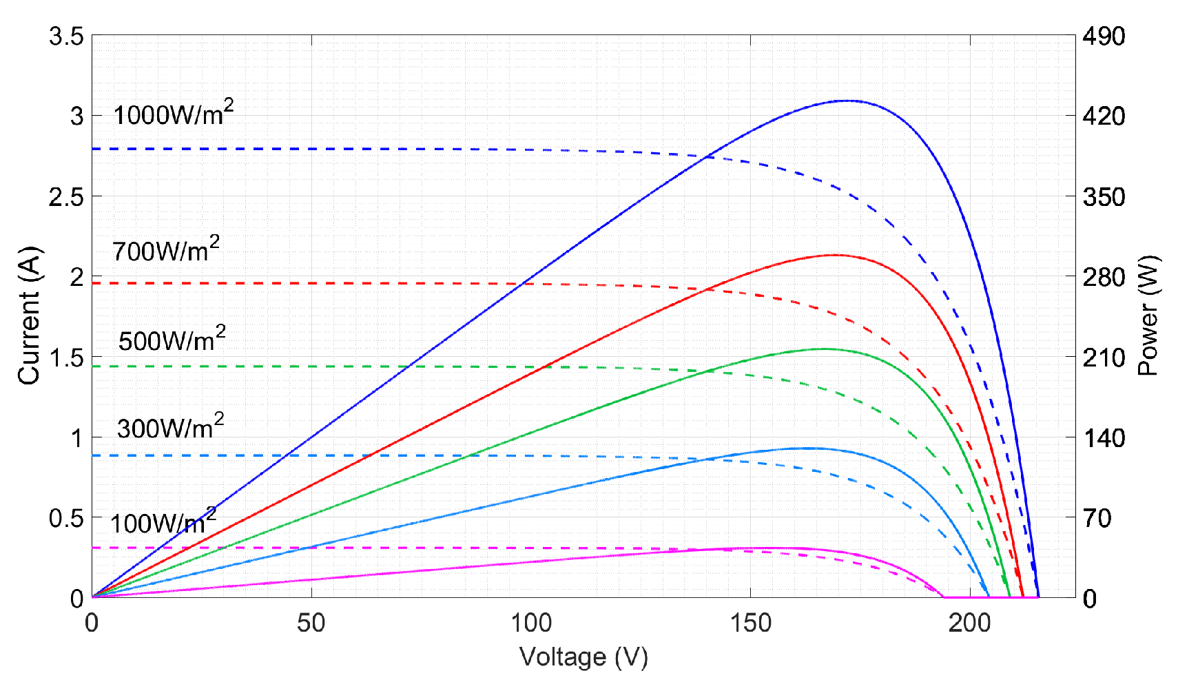
3.1. Simulation Platform
3.2. Initialization
3.3. Convergence Criteria
3.4. Final Remark
4. Conclusions
Author Contributions
Funding
Acknowledgments
Conflicts of Interest
Appendix A
References
- McCrone, A.; Moslener, U.; d’Estais, F.; Gruning, C. Global Trends in Renewable Energy Investment 2017; Frankfurt School-UNEP Centre/BNEF: Frankfurt am Main, Germany, 6 April 2017; pp. 1–90. [Google Scholar]
- International Energy Agency. Global trends in renewable energy investment 2017. In Tracking Clean Energy Progress 2017; International Energy Agency: Paris, France, 2017; pp. 1–112. [Google Scholar]
- Teng, J.H.; Huang, W.H.; Hsu, T.A.; Wang, C.Y. Novel and Fast Maximum Power Point Tracking for Photovoltaic Generation. IEEE Trans. Ind. Electron. 2016, 63, 4955–4966. [Google Scholar] [CrossRef]
- Pilawa-Podgurski, R.C.N.; Perreault, D.J. Sub-module integrated distributed maximum power point tracking for solar photovoltaic applications. In Proceedings of the IEEE Energy Conversion Congress and Exposition (ECCE), Raleigh, NC, USA, 5–20 September 2012; pp. 4776–4783. [Google Scholar]
- Poshtkouhi, S.; Varley, J.; Popuri, R.; Trescases, O. Analysis of distributed peak power tracking in photovoltaic systems. In Proceedings of the 2010 International Power Electronics Conference-ECCE ASIA, Sapporo, Japan, 21–24 June 2010; pp. 942–947. [Google Scholar]
- Luo, H.; Wen, H.; Li, X.; Jiang, L.; Hu, Y. Synchronous buck converter based low-cost and high-efficiency sub-module DMPPT PV system under partial shading conditions. Energy Convers. Manag. 2016, 126, 473–487. [Google Scholar] [CrossRef]
- Birane, M.; Larbes, C.; Cheknane, A. Comparative study and performance evaluation of central and distributed topologies of photovoltaic system. Int. J. Hydrog. Energy 2017, 42, 8703–8711. [Google Scholar] [CrossRef]
- Poshtkouhi, S.; Palaniappan, V.; Fard, M.; Trescases, O. A General Approach for Quantifying the Benefit of Distributed Power Electronics for Fine Grained MPPT in Photovoltaic Applications Using 3-D Modeling. IEEE Trans. Power Electron. 2012, 27, 4656–4666. [Google Scholar] [CrossRef]
- Amir, A.; Amir, A.; Selvaraj, J.; Rahim, N. Study of the MPP tracking algorithms: Focusing the numerical method techniques. Renew. Sustain. Energy Rev. 2016, 62, 350–371. [Google Scholar] [CrossRef]
- Danandeh, M.A.; Mousavi, S.M.G. Comparative and comprehensive review of maximum power point tracking methods for PV cells. Renew. Sustain. Energy Rev. 2018, 82, 2743–2767. [Google Scholar] [CrossRef]
- Eltawil, M.A.; Zhao, Z. MPPT techniques for photovoltaic applications. Renew. Sustain. Energy Rev. 2013, 25, 793–813. [Google Scholar] [CrossRef]
- Bendib, B.; Belmili, H.; Krim, F. A survey of the most used MPPT methods: Conventional and advanced algorithms applied for photovoltaic systems. Renew. Sustain. Energy Rev. 2015, 45, 637–648. [Google Scholar] [CrossRef]
- Subudhi, B.; Pradhan, R. A Comparative Study on Maximum Power Point Tracking Techniques for Photovoltaic Power Systems. IEEE Trans. Sustain. Energy 2013, 4, 89–98. [Google Scholar] [CrossRef]
- Kimball, J.W.; Krein, P.T. Discrete-Time Ripple Correlation Control for Maximum Power Point Tracking. IEEE Trans. Power Electron. 2008, 23, 2353–2362. [Google Scholar] [CrossRef]
- Wasynezuk, O. Dynamic Behavior of a Class of Photovoltaic Power Systems. IEEE Trans. Power Appl. Syst. 1983, PAS-102, 3031–3037. [Google Scholar] [CrossRef]
- Kjær, S.B. Evaluation of the Hill Climbing and Incremental Conductance Maximum Power Point Trackers for Photovoltaic Power Systems. IEEE Trans. Energy Convers. 2012, 27, 922–929. [Google Scholar] [CrossRef]
- Samantara, S.; Roy, B.; Sharma, R.; Choudhury, S.; Jena, B. Modeling and simulation of integrated CUK converter for grid connected PV system with EPP MPPT hybridization. In Proceedings of the 2015 IEEE Power, Communication and Information Technology Conference (PCITC), Bhubaneswar, India, 15–17 October 2015; pp. 397–402. [Google Scholar] [CrossRef]
- Ahmed, J.; Salam, Z. A Modified P O Maximum Power Point Tracking Method with Reduced Steady-State Oscillation and Improved Tracking Efficiency. IEEE Trans. Sustain. Energy 2016, 7, 1506–1515. [Google Scholar] [CrossRef]
- Liu, F.; Duan, S.; Liu, F.; Liu, B.; Kang, Y. A Variable Step Size INC MPPT Method for PV Systems. IEEE Trans. Ind. Electron. 2008, 55, 2622–2628. [Google Scholar] [CrossRef] [Green Version]
- Chu, C.C.; Chen, C.L. Robust maximum power point tracking method for photovoltaic cells: A sliding mode control approach. Sol. Energy 2009, 83, 1370–1378. [Google Scholar] [CrossRef]
- Liu, Y.; Chen, L.; Chen, L.; Xin, H.; Gan, D. A newton quadratic interpolation based control strategy for photovoltaic system. In Proceedings of the International Conference on Sustainable Power Generation and Supply (SUPERGEN 2012), Hangzhou, China, 8–9 September 2012; pp. 1–6. [Google Scholar] [CrossRef]
- Pai, F.S.; Chao, R.M.; Ko, S.H.; Lee, T.S. Performance Evaluation of Parabolic Prediction to Maximum Power Point Tracking for PV Array. IEEE Trans. Sustain. Energy 2011, 2, 60–68. [Google Scholar] [CrossRef]
- Wang, P.; Zhu, H.; Shen, W.; Choo, F.H.; Loh, P.C.; Tan, K.K. A novel approach of maximizing energy harvesting in photovoltaic systems based on bisection search theorem. In Proceedings of the 2010 Twenty-Fifth Annual IEEE Applied Power Electronics Conference and Exposition (APEC), Palm Springs, CA, USA, 21–25 February 2010; pp. 2143–2148. [Google Scholar] [CrossRef]
- Zhang, Q.; Hu, C.; Chen, L.; Amirahmadi, A.; Kutkut, N.; Shen, Z.J.; Batarseh, I. A Center Point Iteration MPPT Method with Application on the Frequency-Modulated LLC Microinverter. IEEE Trans. Power Electron. 2014, 29, 1262–1274. [Google Scholar] [CrossRef]
- Chun, S.; Kwasinski, A. Analysis of Classical Root-Finding Methods Applied to Digital Maximum Power Point Tracking for Sustainable Photovoltaic Energy Generation. IEEE Trans. Power Electron. 2011, 26, 3730–3743. [Google Scholar] [CrossRef]
- Hosseini, S.H.; Farakhor, A.; Haghighian, S.K. Novel algorithm of maximum power point tracking (MPPT) for variable speed PMSG wind generation systems through model predictive control. In Proceedings of the 2013 8th International Conference on Electrical and Electronics Engineering (ELECO), Bursa, Turkey, 28–30 November 2013; pp. 243–247. [Google Scholar] [CrossRef]
- Xiao, W.; Dunford, W.G.; Palmer, P.R.; Capel, A. Application of Centered Differentiation and Steepest Descent to Maximum Power Point Tracking. IEEE Trans. Ind. Electron. 2007, 54, 2539–2549. [Google Scholar] [CrossRef]
- Jamil, M.; Saeed, H.; Qaisar, S.; Felemban, E.A. Maximum power point tracking of a solar system using state space averaging for wireless sensor network. In Proceedings of the 2013 IEEE International Conference on Smart Instrumentation, Measurement and Applications (ICSIMA), Kuala Lumpur, Malaysia, 25–27 November 2013; pp. 1–6. [Google Scholar] [CrossRef]
- Miyatake, M.; Veerachary, M.; Toriumi, F.; Fujii, N.; Ko, H. Maximum Power Point Tracking of Multiple Photovoltaic Arrays: A PSO Approach. IEEE Trans. Aerosp. Electron. Syst. 2011, 47, 367–380. [Google Scholar] [CrossRef]
- Shao, R.; Wei, R.; Chang, L. A multi-stage MPPT algorithm for PV systems based on golden section search method. In Proceedings of the 2014 IEEE Applied Power Electronics Conference and Exposition-APEC 2014, Fort Worth, TX, USA, 16–20 March 2014; pp. 676–683. [Google Scholar] [CrossRef]
- Kiefer, J. Sequential Minimax Search for a Maximum. Proc. Am. Math. Soc. 1953, 4, 502–506. [Google Scholar] [CrossRef]
- Shao, R.; Chang, L. A new maximum power point tracking method for photovoltaic arrays using golden section search algorithm. In Proceedings of the 2008 Canadian Conference on Electrical and Computer Engineering, Niagara Falls, ON, Canada, 4–7 May 2008; pp. 000619–000622. [Google Scholar] [CrossRef]
- Mathews, J.; Fink, K. Numerical Methods Using MATLAB; Featured Titles for Numerical Analysis Series; Pearson Prentice Hall: Upper Saddle River, NJ, USA, 2004. [Google Scholar]
- Ropp, M.E.; Gonzalez, S. Development of a MATLAB/Simulink Model of a Single-Phase Grid-Connected Photovoltaic System. IEEE Trans. Energy Convers. 2009, 24, 195–202. [Google Scholar] [CrossRef]
- Kumar, N.; Hussain, I.; Singh, B.; Panigrahi, B.K. Self-Adaptive Incremental Conductance Algorithm for Swift and Ripple Free Maximum Power Harvesting from PV Array. IEEE Trans. Ind. Inf. 2018, 14, 2031–2041. [Google Scholar] [CrossRef]
- Elgendy, M.A.; Zahawi, B.; Atkinson, D.J. Assessment of the Incremental Conductance Maximum Power Point Tracking Algorithm. IEEE Trans. Sustain. Energy 2013, 4, 108–117. [Google Scholar] [CrossRef]
- Femia, N.; Petrone, G.; Spagnuolo, G.; Vitelli, M. Optimizing duty-cycle perturbation of P&O MPPT technique. In Proceedings of the 2004 IEEE 35th Annual Power Electronics Specialists Conference (IEEE Cat. No. 04CH37551), Aachen, Germany, 20–25 June 2004; Volume 3, pp. 1939–1944. [Google Scholar] [CrossRef]
- European Committee for Electrotechnical Standardization. Overall Efficiency of Grid Connected Photovoltaic Inverters; BSI: Brussels, Belgium, 2010. [Google Scholar]


| Parameters | Value |
|---|---|
| Maximum Power () | 39.318 W |
| Open Circuit Voltage () | 19.6 V |
| Maximum Power Voltage () | 15.634 V |
| Short Circuit Current () | 2.79 A |
| Maximum Power Current () | 2.5149 A |
| Temperature Coefficient () | /K |
| Types of DMPPT | Initialization | Effect of Initialization toward Accuracy | Survivability under Rapid Change of Irradiance | Transient Fluctuation | FLOPs | Convergence Criteria | |
|---|---|---|---|---|---|---|---|
| P&O | PBM | 1 | Not affecting | Excellent | Small | 11 | No required |
| INC | CM | 1 | Not affecting | Excellent | Small | 11 | No required |
| GSS | BBM | 2 | Affecting | Poor | Big | 11 | Required |
| NQI | IBM | 3 | Affecting | Poor | Varies | 19 | Required |
© 2018 by the authors. Licensee MDPI, Basel, Switzerland. This article is an open access article distributed under the terms and conditions of the Creative Commons Attribution (CC BY) license (http://creativecommons.org/licenses/by/4.0/).
Share and Cite
Andrean, V.; Chang, P.C.; Lian, K.L. A Review and New Problems Discovery of Four Simple Decentralized Maximum Power Point Tracking Algorithms—Perturb and Observe, Incremental Conductance, Golden Section Search, and Newton’s Quadratic Interpolation. Energies 2018, 11, 2966. https://doi.org/10.3390/en11112966
Andrean V, Chang PC, Lian KL. A Review and New Problems Discovery of Four Simple Decentralized Maximum Power Point Tracking Algorithms—Perturb and Observe, Incremental Conductance, Golden Section Search, and Newton’s Quadratic Interpolation. Energies. 2018; 11(11):2966. https://doi.org/10.3390/en11112966
Chicago/Turabian StyleAndrean, Victor, Pei Cheng Chang, and Kuo Lung Lian. 2018. "A Review and New Problems Discovery of Four Simple Decentralized Maximum Power Point Tracking Algorithms—Perturb and Observe, Incremental Conductance, Golden Section Search, and Newton’s Quadratic Interpolation" Energies 11, no. 11: 2966. https://doi.org/10.3390/en11112966