Double Layer Dynamic Game Bidding Mechanism Based on Multi-Agent Technology for Virtual Power Plant and Internal Distributed Energy Resource

Abstract

As renewable energies become the main direction of global energy development in the future, Virtual Power Plant (VPP) becomes a regional multi-energy aggregation model for large-scale integration of distributed generation into the power grid. It also provides an important way for distributed energy resources (DER) to participate in electricity market transactions. Firstly, the basic concept of VPP is outlined, and various uncertainties within VPP are modeled. Secondly, using multi-agent technology and Stackelberg dynamic game theory, a double-layer nested dynamic game bidding model including VPP and its internal DERs is designed. The lower layer is a bidding game for VPP internal market including DER. VPP is the leader and each DER is a subagent that acts as a follower to maximize its profit. Each subagent uses the particle swarm algorithm (PSA) to determine the optimal offer coefficient, and VPP carries out internal market clearing with the minimum variance of unit profit according to the quoting results. Then, the subagents renew the game to update the bidding strategy based on the outcomes of the external and internal markets. The upper layer is the external market bidding game. The trading center (TC) is the leader and VPP is the agent and the follower. The game is played with the goal of maximum self-interest. The agent uses genetic algorithms to determine the optimal bid strategy, and the TC carries out market clearance with the goal of maximizing social benefits according to the quotation results. Each agent renews the game to update the bidding strategy based on the clearing result and the reporting of the subagents. The dynamic game is repeated until the optimal equilibrium solution is obtained. Finally, the effectiveness of the model is verified by taking the IEEE30-bus system as an example.

1. Introduction

With the continuous increase of power demand and the increasingly severe problems of global energy shortages and environmental pollution, distributed generations (DG) have been adopted by more and more countries due to their reliability, economy, flexibility and environmental protection.

Nowadays, the global power industry is rapidly transforming, and the power system should be based on market operations. However, because of the characteristics of DG, such as small capacity and being random, intermittent and volatile, it is not feasible for them to join power market operations alone. At present, most studies use the concept of microgrid (MG) as the grid connection form of DG [1]. MG can well coordinate the technical contradiction between large power grids and DGs, and has certain energy management functions. However, MG takes the local application of DGs and users as the main control target, and is subject to geographical restrictions. There are also some limitations on the effective use of multi-regional and large-scale DGs and the economies of scale in the power market [2]. The concept of Virtual Power Plant (VPP)-provides new ideas for solving these problems.

The term “virtual power plant” is derived from Dr. Shimon Awerbuch’s book “Virtual Public Facilities: Description, Technology, and Competitiveness of Emerging Industries” [3]. VPP does not change the way each DG is connected to the grid. Instead, it uses advanced technologies such as metrology and communications to aggregate DGs and energy storage systems. Different types of distributed energy resources, such as controllable loads and electric vehicles (EV), achieve coordinated and optimized operation through higher-level software architecture, which is more conducive to the rational allocation and utilization of resources. This method can aggregate DERs without transforming the power grid, and provides stable power transmission to the power grid, becoming an effective method for DERs to join the power market, reducing the risk of their independent operation in the market and the impact of grid-connected DER on the power grid [4,5,6,7].

The existing research of VPP focuses on two aspects: one is optimizing the internal resources of a single VPP, and the other is participating in overall power system dispatch. In terms of VPP internal resource allocation, Sun S. et al. [8] studied the VPP optimization scheduling model with EV, using direct, hierarchical and distributed methods to control the charging and discharging of EV. Zhao H. et al. [9] constructed an internal VPP scheduling model with interruptible load, and determined the VPP optimization scheduling model with uncertain wind power through scene analysis method. Liu Y.Y. et al. [10] established a bidding model for VPP and considered uncertainty to solve the VPP optimal scheduling problem under multi-market mode. Zamani A.G. et al. [11] considered the energy storage system and demand response, established the VPP optimization scheduling model, and conducted the related researches on the VPP bidding problem. Zang H.X. et al. [12] divided the VPP into incentive demand-responsive VPP and price demand-responsive VPP according to the internal demand response type, and established a day-ahead dispatch model considering the demand response. Guo H.X. et al. [13] constructed a bidding model for VPP. However, the VPP studied was only used as a price receiver and could not affect the outcome of system clearing. Its essence is still the internal optimization problem of a virtual power plant.

In the context of VPP’s participation in competition in the electricity market, Rahimiyan M. and Baringo L. [14] considered the electricity market under the hybrid model. A VPP that includes wind farms, pumped storage power plants, and gas turbines participates in the operation of the medium-term contract market, daily market, and balance market. Mnatsakanyan A. and Kennedy S.W. [15] proposed a bidding model in which VPP participates in the energy market and ancillary service markets, and determined the bidding power of VPP in each market. Liu J.N. et al. [16] adopted the point estimation method to deal with the uncertainty of electricity price and new energy generation, and proposed a bidding strategy of VPP in the current electricity market. Song W. et al. [17] considered the power supply-demand balance and safety constraints of VPP, and put forward the joint bidding model of VPP in the power energy and hot standby market. Yang J.J. et al. [18] considered the uncertainty of the EVs’ number and wind generations’ power, and established a robust optimization model for VPP to participate in the day-ahead energy market and regulate market bidding. Peik-Herfeh M. et al. [19] reviewed the participation of VPP in the electricity market, and compared and analyzed the similarities and differences between VPP and MG. Fang Y.Q. et al. [20] used game theory to study the participation of multiples VPPs in the electricity market. VPPs mainly include distributed generation, energy storage, and time-of-use electricity price demand responses. Mashhour E. and Moghaddas-Tafreshi S.M. [21,22] studied the VPP participating in the main energy and ancillary service markets theoretically, and established a non-equilibrium model that considered the demand response and the VPP safety constraints. Zhou Y.Z. et al. [23] introduced agency theory and used energy storage of EV to reduce the impact of randomness of wind power on the system. VPP participated in the electricity market as a whole and responded to market price information. Yuan G.L. et al. [24] proposed a multi-agent power market simulation mechanism using game theory and machine learning methods, and used scene analysis methods to analyze the market behavior of VPPs. Wang Y. et al. [25] took maximizing the profit of day-ahead market bidding and balancing market reward as goals. A commercial VPP model that considered interruptible loads, small wind farms, pumped storage power stations, and gas turbines was established.

However, in the operation of VPP, different types of DER are most likely to belong to different owners of property rights. Conventionally, it is no longer appropriate to consider VPP as a whole to participate in bidding. Therefore, it is necessary to consider the independence of internal entities and study bidding issues involving multiple types of DER from multiple entities. To guide VPP to occupy a more favorable position in the power market competition, and maximize its internal DER interests, this paper establishes a double-layer nested Stackelberg dynamic game model based on multi-agent technology. In Section 2, based on analyzing the main structure of VPP, a probabilistic output model for various uncertainties within VPP is established. In Section 3, multi-agent technology and Stackelberg dynamic game theory are used to design the underlying VPP internal market bidding mechanism, and establish the dynamic game model of each DER subagent. In combination with the real-time clearing results of the lower layer games, a multi-agent day-before-day power market dynamic game model with VPP is designed. Through repeated games, until the upper and lower levels jointly clear out, and obtain the optimal bid strategy of VPPs and its internal DERs. In Section 4, an IEEE 9 system is used as an example to demonstrate the validity of the proposed model and method. Section 5 contains some conclusions about the research.

2. Uncertain Factors Modeling in VPP

The VPP studied in this paper contains wind turbine (WT), photovoltaic (PV), energy storage (ES) devices, demand side resources (DSR), and diesel generators (DE). The power of DE is controllable, and the internal uncertainty of VPP mainly comes from the prediction error and random fluctuation of each DER, ES device and various loads.

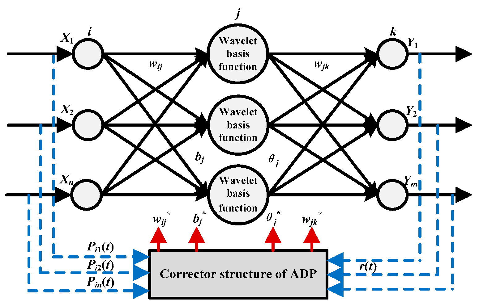
2.1. Error Correction Based Fixed Load and DER Output Prediction

When forecasting the output of fixed load and DERs (PV and WT), this paper uses modified wavelet neural network (WNN) prediction method [26] which adds additional adaptive dynamic programming correction links. The idea of “prediction–correction” is introduced, and actual measurement data are used to update the WNN parameters to improve the prediction accuracy. The prediction principle is shown in Figure 1.

In the VPP model diagram, x₁, x₂, …, x_n are input parameter sequences; Y₁, Y₂, …, Y_m are output parameter sequences; $w_{ij}$ is the weight of the input layer to the hidden layer; $w_{jk}$ is the weight value from the hidden layer to the output layer; $b_j$ is the wavelet basis function scaling factor; θ is the threshold; P_i1(t), P_i2(t), …, P_in(t) are the measured data during the sampling period; $w_{ij}^{\ast }$, $w_{jk}^{\ast }$, $b_j^{\ast }$ and ${\theta }_j^{\ast }$ are updated parameter of the optimized structure using adaptive dynamic programming; and r(t) is the cost function.

The specific process for forecasting using the WNN model is as follows:

Step 1:

Pre-process data; cull or correcti bad data in various types of data; and normalizing them.

Step 2:

Determine the number of nodes n, l and m of the WNN input layer, the hidden layer, and the output layer according to the original data (where the number of hidden layer nodes adopts an empirical value, that is, the default l = 2n − 1), and determine the maximum iteration (number of times N_max and iteration accuracy e₀).

Step 3:

Randomly initialize the weights of the WNN (input layer to implicit layer weight wij and implicit layer to output layer weight w_jk) and wavelet basis function related parameters (scaling factor a_j and translation factor b_j), that is, w_ij = randn (n,l), w_jk = randn (l,m), a_j = randn (1,l) and b_j = randn (1,l).

Step 4:

Initialize the learning rates η1 and η2 of w_ij and w_jk (both defaults to 0.01) and the learning rates η3 and η4 of a_j and b_j (both default to 0.001).

Step 5:

Input the pre-processed data obtained in Step 1 into the WNN. Meanwhile, input the measured data of the sampling period and the obtained neural network output sequence into the ADP correction optimization structure. Obtain network weights w^*_ij and w^*_jk with strong fitting ability for the original data and wavelet parameters a^*_j and b^*_j.

Step 6:

Input the data used for the prediction into the trained WNN network, obtain the predicted value by prediction, calculate the error, and derive the prediction result and analyze it.

2.1.1. Fixed Load Forecast

According to the statistical theory of probability, the normal distribution (ND) has good properties and can be used to approximate many probability distributions. Therefore, the ND is used to estimate the error caused by the fixed load forecast.

2.1.2. WT Forecast

For the error produced by WT output forecasting, the actual forecasting error of WT shows a large kurtosis and skewness, and simply using the normal distribution description will produce a larger error. Wang et al. [27] pointed out that the wind speed prediction error was the main cause of the WT forecasting error, and the different WT forecasting values corresponding to the WT forecast error had different probability distributions. The article also gives the applicable wind speed interval (m/s) for different distributions: the applicable range of the “0 error” distribution is [0, 2.1], [12.6, ∞]; the applicable range of the exponential distribution is (2.1, 5.1]; the ND applies to (5.1, 9.8); and the extreme value distribution applies to [9.8, 12.6). This paper draws on the idea of the literature and uses the error distribution of the corresponding wind speed to establish different probability density functions to estimate the error produced by WT output prediction.

2.1.3. PV Forecast

For the error generated by PV output prediction, simply using the ND description will also produce a larger error. Yadav et al. [28] pointed out that the output level of photovoltaic power generation is closely related to the weather conditions, and the distribution of forecast error under different weather types is different. This paper draws on the idea of the literature, and uses the idea of different weather types to establish different probability density distribution functions to estimate the error generated by PV output prediction.

2.2. Demand Response Modeling

This paper considers transfer load (TL) and incentive-based interruptible load (IL) based on time-sharing price (TP) mechanism.

2.2.1. Transfer Load

The usage of TL is affected by the real-time electricity price, and a considerable proportion of it will fluctuate with the electricity price with a certain probability. The proportion of TL defined by the tariff is the load transfer rate α_TL [29].

The relationship between TL usage and electricity price C(t) at time t is shown in Equation (1).

$$P_{\mathrm{TL}}(t)={\alpha }_{\mathrm{TL}}(t){P^{\prime }}_{\mathrm{TL}}(t)k+(1-{\alpha }_{\mathrm{TL}}(t)){P^{\prime }}_{\mathrm{TL}}(t)$$

(1)

$$k={\left(\frac{C(t)}{C_{\mathrm{TL}}}\right)}^{\beta }$$

(2)

where P_TL(t) is the total amount of TL after transfer at time t; α_TL(t) is the load transfer rate of TL at time t; P’_TL(t) is the total amount of TL that does not transfer at time t; k is the influence coefficient of electricity price to TL; C_TL is the threshold electricity price of TL transfer and transfer; and β is the demand price elasticity coefficient.

Assuming that the total electricity demand of users within one day is constant, the controlled demand that is reduced in one period will be delayed to other periods. Therefore, the sum of changes in TL usage within one day should be zero, as shown in Equation (3).

$$\begin{array}{ll}\hfill {\displaystyle \sum _{t=1}^{24}\Delta P_{\mathrm{TL}}}(t)& ={\displaystyle \sum _{t=1}^{24}(P_{\mathrm{TL}}(t)-{P^{\prime }}_{\mathrm{TL}}(t))}\hfill \\ & ={\displaystyle \sum _{t=1}^{24}{\alpha }_{\mathrm{TL}}(t)}{P^{\prime }}_{\mathrm{TL}}(t)(k-1)=0\hfill \end{array}$$

(3)

Considering TL access, P’_TL(t) ≠ 0, thus obtaining Equation (4).

$${\displaystyle \sum _{t=1}^{24}{\alpha }_{\mathrm{TL}}(t)(k-1)=0}$$

(4)

In addition, β is usually less than −1, so, when C(t) > C_TL, that is, TL is in roll-out state, k < 1. When C(t) < C_TL, TL is in transition state, k > 1. In view of this, using the NDs of two different parameters to carry out probabilistic modeling of the load transfer rate α_TL at the time of TL roll-out and TL transition, Equation (4) can be modified as Equation (5).

$${\displaystyle \sum _{t\in T_{\mathrm{I}}}{\alpha }_{\mathrm{TL},\mathrm{I}}}(t)(k-1)={\displaystyle \sum _{t\in T_{\mathrm{O}}}{\alpha }_{\mathrm{TL},\mathrm{O}}}(t)(1-k)$$

(5)

where T_I and T_O are the collections of TL transfer in and out in a day, respectively; and α_TL,I and α_TL,O are the load transfer rates when TL is transferred in and out, respectively.

Since the α_TL is sampled according to its probability density function, when the number of samples is large, the sample mean will be close to the expectation of its probability density function. Thus, Equation (5) can be further reduced to:

$$\gamma =\frac{{\mu }_{\mathrm{TL},\mathrm{I}}}{{\mu }_{\mathrm{TL},\mathrm{I},\mathrm{O}}}\approx \frac{t_{\mathrm{O}}{\displaystyle \sum _{t\in T_{\mathrm{O}}}^{}(1-k)}}{t_{\mathrm{I}}{\displaystyle \sum _{t\in T_I}^{}(k-1)}}$$

(6)

where γ is the ratio coefficient between the expected μ_TL,I and μ _TL,O of the distribution α _TL,I and α _TL,O; and t_I and t_O are the number of times included in T_I and T_O, respectively.

When the next day electricity price is known, the threshold price set value, γ, is constant.

2.2.2. Interruptible Load

IL users can sign contracts with power companies to allow them to interrupt power supply under different specific conditions. In this paper, the power-off condition is characterized by the power-off electricity price threshold. Before interrupting the power supply to the IL, the prediction method is the same as the fixed load, and the prediction error is fitted by using the normal distribution. Define S_IL as the 0–1 state variable of IL, and characterize the actual use of IL [29], as shown in Equation (7).

$$S_{IL}(t)=\{\begin{array}{l}0, C(t)\ge C_{IL}\\ 1, C(t)<C_{IL}\end{array}$$

(7)

where S_IL(t) is a state variable at time t; C(t) is a real-time electricity price at time t; and C_IL is a power-off valve price.

2.3. Energy Storage Unit Modeling

The ES unit can be charged and discharged within its allowable range. To extend its service life, it is generally not allowed to overcharge. The basic model of ES is as follows:

$$\{\begin{array}{c}\mathrm{SOC}\left(t\right) = \mathrm{SOC}(t-1) + \Delta {\mathrm{SOC}}_{\mathrm{ch}}(t),t\in T_{\mathrm{ch}}\hfill \\ \mathrm{SOC}\left(t\right) = \mathrm{SOC}(t-1) + \Delta {\mathrm{SOC}}_{\mathrm{dis}}(t),t\in T_{\mathrm{dis}}\hfill \end{array}$$

(8)

$$\{\begin{array}{c}{\mathrm{SOC}}_{\mathrm{ch}}\left(t\right) = P_{\mathrm{ch}}(t){\eta }_{\mathrm{ch}}\Delta T{S}_{\mathrm{es}}(t)/S_{\mathrm{ES}},t\in T_{\mathrm{ch}}\hfill \\ {\mathrm{SOC}}_{\mathrm{dis}}\left(t\right) = P_{\mathrm{dis}}(t){\eta }_{\mathrm{dis}}\Delta T{S}_{\mathrm{es}}(t)/S_{\mathrm{ES}},t\in T_{\mathrm{dis}}\hfill \end{array}$$

(9)

$$\{\begin{array}{c}{S}_{\mathrm{es}}=1,{\lambda }_{\mathrm{es}}<{\lambda }_0\hfill \\ S_{\mathrm{es}}=0,{\lambda }_{\mathrm{es}}<{\lambda }_0\hfill \end{array}$$

(10)

where SOC(t) and SOC(t − 1) are the charge states of the ES device at t and t − 1, respectively; ΔSOC_ch (t) and ΔSOC_dis(t) are the charging and discharging capacities of ES at time t; P_ch(t) and P_dis(t) are charging and discharging powers of ES at time t; η_ch and η_dis are charging and discharging efficiency of ES,; S_ES is rated capacity of ES; S_es(t) is the charging and discharging state parameter of ES at time t; λ_es(t) is the charging and discharging action parameter of ES at time t; λ₀ is the charging and discharging action parameter threshold of ES; and T_ch and T_dis are the charging and discharging time periods of ES, where they are equivalent to the peak time of the electricity price T_f and the time interval of the electricity price valley T_g, respectively.

The charging and discharging rules of the ES are closely related to the price of electricity. The relationship between the charging and discharging power at time t and the price C(t) is shown in Equation (11).

$$\{\begin{array}{l}{P}_{\mathrm{ch}}(t)=a_{\mathrm{ch}}C(t)+b_{\mathrm{ch}},t\in T_{\mathrm{ch}}\hfill \\ P_{\mathrm{dis}}(t)=a_{\mathrm{dis}}C(t)+b_{\mathrm{dis}},t\in T_{\mathrm{dis}}\hfill \end{array}$$

(11)

where a_ch, b_ch, a_dis and b_dis are the relation coefficients of the charging price and the charging and discharging power at the charging time and the discharging time, respectively.

The ES element’s initial charge state is SOC (1) = 0, and the charge state returns to zero at the end of each day, that is, SOC (24) = 0. Thus, all ESs will be completely discharged when the price of electricity peaks at the end of the day. If there is an ES with a non-zero amount of electricity, when the end time of the discharge period is the length of time required for its current discharge, it is forcibly discharged to restore the initial state of charge.

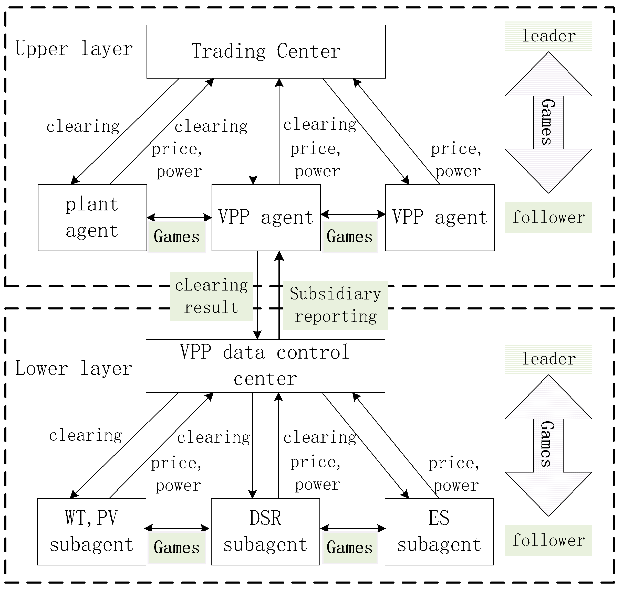
3. Double Layer Bidding Model Design Based on Stackelberg Dynamic Game

3.1. Framework Design of Double Layer Bidding Model

Agents in this paper refer to VPPs and traditional thermal power plants. Subagents refer to various investment entities within VPPs. Multiple VPPs and traditional thermal power plants participate in the day-ahead market bidding of the power system, and each DER only participates in the VPP internal day-ahead market auctions to which it belongs. The market is divided into 24 periods, and only one period is selected when building a model. The software used in the model solving process is “Matlab 2014a”.

The Stackelberg dynamic game bidding model established in this paper can be divided into two layers, where one layer nests a game mode. The lower layer is VPP internal day-ahead market bidding stage. Each DER within the VPP acts as a subagent to obtain forecasted output values based on historical data. The Monte Carlo method is used to generate the quote scenario set and determine the quoted coefficient, and the bid strategy is obtained and submitted to the VPP data center. The VPP data center predicts the load demand based on historical data, and carries out unified internal market clearing. Before the bidding deadline, each subagent may make new bidding strategies.

At the upper layer, VPP acts as an agent to participate in the day-ahead market bidding of the power system with other agents. At this point, the output of VPP is the total power of the internal market in the lower layer, and the unit cost is the clear price of the internal market. Each agent simulated the game through the genetic algorithm (GA) to determine the bidding strategy and reported it to the TC for unified market clearing. Before the bidding deadline, each agent can update the bidding strategy to obtain the best result. The specific model framework is shown in Figure 2.

3.2. Design of VPP Internal Bidding Model Based on Dynamic Game

After each subagent in VPP conducts the first round of game, it reports to the VPP data control center the availability and quotation for each period. The VPP data control center carries out the unified internal market clearing, that is, the selection of the power generation sequence from low to high electricity prices until the supply and demand balance is satisfied. After determining the clear price and the clearing power quantity, the information is fed back to each subagent. Each subagent formulates a new bidding strategy based on the feedback information, so that the game is repeated until an optimal equilibrium strategy is obtained.

3.2.1. Bidding Strategy of Subagent in VPP Internal Market

This section examines the bid strategies for a single subagent i. Assume that each subagent uses a linear quoting function [30], as shown in Equation (12).

$$P_i(q_i)={\alpha }_i+{\beta }_i{q}_i$$

(12)

where α_i and β_i are quote parameters of the subagent i and q_i is the inflow and outflow power of the subagent i. The specified energy outflow is positive, and the inflow is negative.

In addition to considering operational costs and operational constraints, subagent i must also consider possible quotations from other subagents when quoting. Under normal circumstances, subagent i does not know the price coefficient of the competitor j, and can only perform the probability estimation by using historical information. Under the power market clearing rule, the price coefficient of the subagent j conforms to the two-dimensional normal distribution [31,32], and its probability density function is shown as in Equation (13).

$$({\alpha }_{ij},{\beta }_{ij})\sim N(\left[\begin{array}{l}{\mu }_{\alpha ,ij}\\ {\mu }_{\beta ,ij}\end{array}\right],\left[\begin{array}{cc}{\sigma }_{\alpha ,ij}^2& {\rho }_{ij}{\sigma }_{\alpha ,ij}{\sigma }_{\beta ,ij}\\ {\rho }_{ij}{\sigma }_{\alpha ,ij}{\sigma }_{\beta ,ij}& {\sigma }_{\beta ,ij}^2\end{array}\right])$$

(13)

where the subscript ij represents subagent i’s estimate of subagent j; σ_α,ij and σ_β,ij are the standard deviation estimates of α and β respectively; μ_α,ij and μ_β,ij are mean estimates of α and β, respectively; and ρ_ij is the correlation coefficient between α and β. When subagent i predicts the power of subagent j is negative, ρ_ij is −1. As a supplier of electric energy, to increase the number of successful bids, one factor will be increased while the other coefficient will be decreased. Similarly, it can be obtained that when j needs to purchase electricity from the outside, the ρ_ij is 1.

Subagent i can generate subagent j quoting scenario set through Monte Carlo simulation to determine its own optimal bidding strategy. The quota coefficient scene generation step is as follows:

(1)

Step 1: Assuming $M=\left[\begin{array}{cc}{\sigma }_{\alpha ,ij}^2& {\rho }_{ij}{\sigma }_{\alpha ,ij}{\sigma }_{\beta ,ij}\\ {\rho }_{ij}{\sigma }_{\alpha ,ij}{\sigma }_{\beta ,ij}& {\sigma }_{\beta ,ij}^2\end{array}\right]$, the lower triangular matrix A is generated such that M = AA^T.

(2)

Step 2: Producing mutually independent two-dimensional standard normal distribution random vectors λ = [λ_α, λ_β]^T, where λ_α～N (0, 1), λ_β～N (0, 1).

(3)

Step 3: [α_ij, β_ij]^T = [μ_α,ij, μ_β,ij]^T + Aλ.

Each subagent in VPP will pursue its own maximization of profit in the bidding process. The expected profit function of subagent i is as follows:

$$\max E_i=(R_{in}-C_i)\cdot q_i^R$$

(14)

where R_in indicates the price of the VPP internal market at a certain time; q^R_i represents the outgoing power of the agent i at the same time; and C_i is the cost of the subagent i’s power generation.

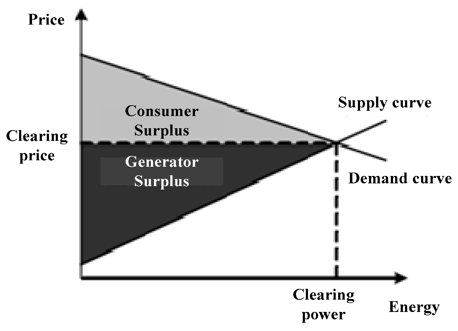
3.2.2. VPP Internal Day-Ahead Market Clearing

During the competition in the VPP internal market, efficient subagents have more advantages because high-performance subagents in the process of re-quotes can sell electricity at a relatively low price and earn profits. Subagents with lower efficiency over time will be eliminated from the internal market. In a small VPP system, this bidding model threatens the balance between supply and demand and standby demand, and it is not conducive to long-term stable operation of the system. This paper adopts the uniform clearing price (UCP) for settlement. When the VPP internal market clears, the goal of pursuing the average of the unit power profit is to ensure that all players are as profitable as possible. Therefore, the clearing result is generated when the variance of the unit‘s profit is the smallest, that is, the bidding strategy that guarantees the safe and stable operation of the VPP internal system in the bidding process is easier to win the bid [33].

Introducing the unit power balance objective of subagent i as follows:

$$\min V={\displaystyle \sum _{i=1}^m{(\overline{V}-V_i)}^2}$$

(15)

$$\overline{V}=\frac{1}{m}(V_1+V_2+\cdots +V_i+\cdots +V_m)$$

(16)

$$V_i=\frac{{\displaystyle \sum _{i=1}^m[{(P_i-C_i)}^2\cdot q_i]}}{{\displaystyle \sum _{i=1}^m{q}_i}}$$

(17)

where the subscript m is the total number of subagents in VPP and V is the subagent’s profit variance of per-unit electricity.

This paper ignores the cost of power generation for WT and PV. Other subagents’ costs are shown in Equations (18)–(21).

$$F^{DE}={\displaystyle \sum _{i\in m}(a{q}_i^{D{E}^2}+b{q}_i^{DE}+c)}$$

(18)

$$F^{DS}=C_{}^C+C_{}^{IL}$$

(19)

$$C_{}^C=\delta \cdot q_{}^C,C_{}^{IL}=\gamma \cdot q_{}^{IL}$$

(20)

$$F^{ES}=\frac{1}{2}e\cdot \left|q^{ES}\right|$$

(21)

where F^DE, F^DS and F^ES are power generation costs of DEs, demand-side response costs, and energy storage operating costs, respectively; $q_i^{D{E}^{}}$ is the power generated by ${}_i^{DE}$ (ith diesel generator in VPP) at a certain moment; a, b, and c are its consumption factors; C^C and C^IL are the interruption capacity costs and interruption cost of VPP at a certain moment; δ and γ are the interrupted capacity prices and interrupted charge prices of VPP at a certain moment; q^C and q^IL represent the interrupt capacity and interrupted power provided by VPP at a certain time; q^ES is the charge or discharge power of the ES device at a certain time, which can be positive or negative; and e is the energy storage cost, which is determined by the energy storage efficiency.

The clearing process includes the following constraints:

(1)

Power balance constraints

$$\begin{array}{l}{Q}^{VPP}=Q_G^{VPP}-Q_L^{VPP}+Q_{IL}^{VPP}\\ Q_G^{VPP}=q^{DE}+q^{WT}+q^{PV}+q^{ES}\end{array}$$

(22)

where Q^VPP indicates the overall external power of VPP at a certain moment. When it is positive, it means that VPP generates electricity to the outside. When it is negative, it means that VPP purchases electricity; $Q_G^{VPP}$ indicates the total power generated by VPP at a certain moment; and q^DE, q^WT, and q^PV, respectively, represent the power generation of all DEs, all WTs, and all PVs at a time.

(2)

Power constraints for WT and PV

$$\begin{array}{l}{q}_{i\min }^{WT}\le q_i^{WT}\le q_{i\max }^{WT}\\ q_{i\min }^{PV}\le q_i^{PV}\le q_{i\max }^{PV}\end{array}$$

(23)

where $q_{i\max }^{WT}$, $q_{\max }^{WT}$ are the upper and lower limits of the external output of ${}_i^{WT}$; and $q_{i\max }^{PV}$ and $q_{\max }^{PV}$ are the upper and lower limits of the external output of ${}_i^{PV}$, respectively.

(3)

Power constraints for DE

$$q_{i\min }^{DE}\le q_i^{DE}\le q_{i\max }^{DE}$$

(24)

$$-\Delta q_i^{down}\le q_{t,i}^{}-q_{t-1,i}^{}\le \Delta q_i^{up}$$

(25)

where $q_{i\max }^{DE}$ and $q_{\min }^{DE}$ are the upper and lower limits of ${}_i^{DE}$ output to a certain moment; and $\Delta q_i^{down}$ and $\Delta q_i^{up}$ are the power variation limits of ${}_i^{DE}$ in pre-unit time, that is, the upper and lower limits of climbing rate.

(4)

Capacity constraints for ES devices

$${\displaystyle \sum _{t\in T}{q}_t^{ES}\cdot \Delta t}=0$$

(26)

where $\Delta t$ is the time interval and T is the charge and discharge cycle.

(5)

Charging and discharging constraints for ES devices

$$E_{\min }\le E_0-{\displaystyle \sum _{i=1}^t{q}_t^{ES}\cdot \Delta t}\le E_{\max }, \mathrm{t}=1, 2, \cdots , \mathrm{T}$$

(27)

$$-q_{\max }^{ch}\le q_{}^{ES}\le q_{\max }^{dis}$$

(28)

where E_max and E_min are the upper and lower limits of the ES device, respectively; and $q_{\max }^{ch}$ and $q_{\max }^{dis}$ are the power limits for ES charging and discharging, respectively.

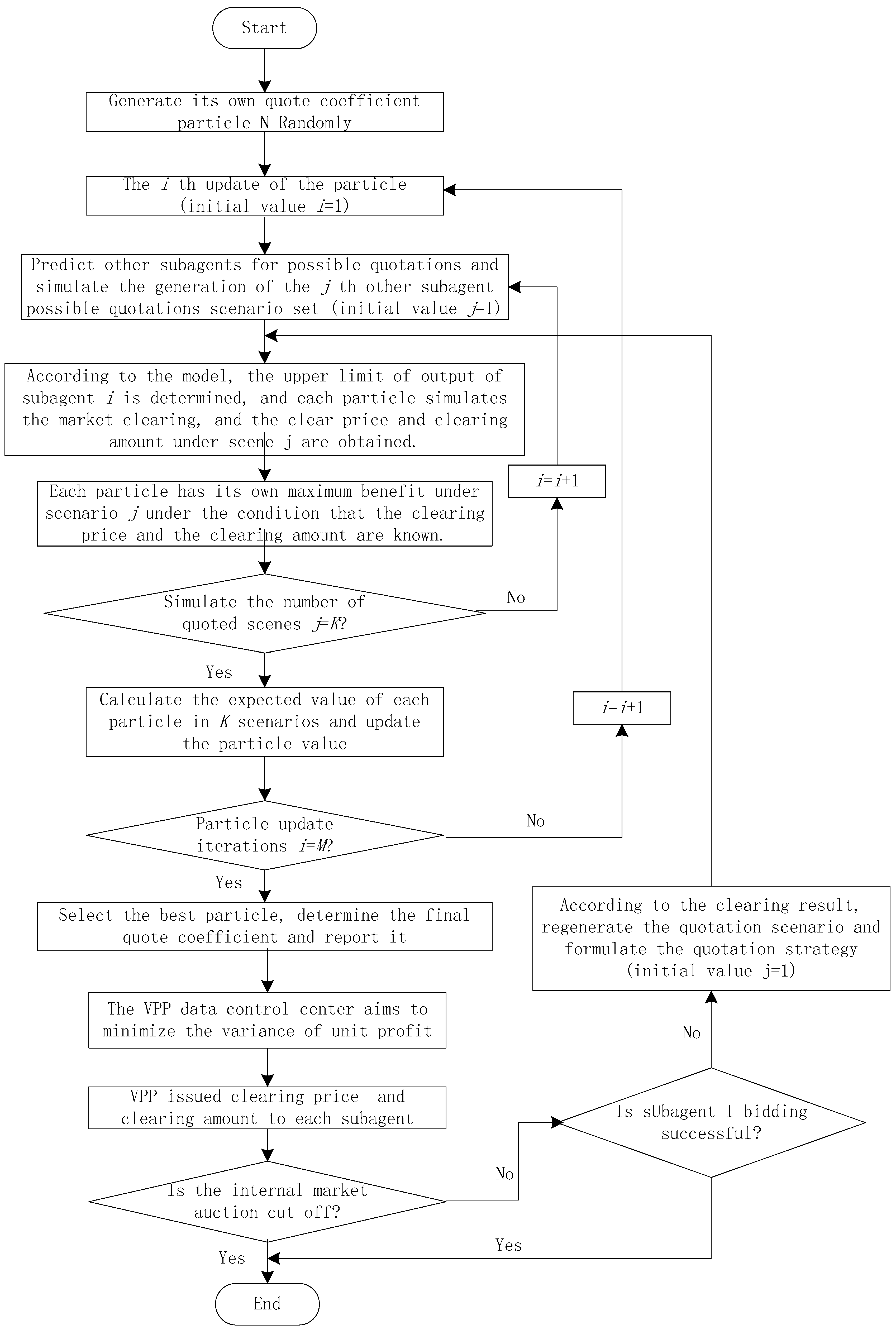
3.2.3. Model Solving

The solution of this section mainly focuses on the determination of the subagent quotation coefficient and the internal market clearing of VPP. The algorithm flow is shown in Figure 3. The PSA is used to solve the optimal quote coefficient. Subagent i simulates and generates a set of possible bid scenarios based on historical bid data of other subagents, and obtains the maximum revenue of the subagent i under each scenario, with the expectation of maximum profit. The target is updated and the particles selected to determine the final quote coefficient. To solve the issue of VPP internal market clearing, the GA toolbox in “Matlab 2014a” was used to solve the problem.

3.3. VPP Dynamic Fame Bidding Model Based on Multi-Agent Technology

3.3.1. Model Establishing

All agents will pursue the maximization of their own interests during the bidding process. For this reason, the function argmax (•) is introduced to represent a set of solution sets in the definition domain. Each set of solutions enables the function argmax (•) to obtain the maximum value. From this, the Objective Function 1 shown in Equation (28) can be obtained.

$$\left\{\begin{array}{c}{P}_1^{VP{P}^{\ast }}\in \underset{P_1^{VPP}}{\arg \max }[(P_1^{VPP}-R_{in})\cdot Q_1(P_1^{VPP}{}_1,\cdots ,P_{n_1}^{VP{P}^{\ast }})]\\ ⋮\\ P_{n_1}^{VP{P}^{\ast }}\in \underset{P_{n_1}^{VPP}}{\arg \max }[(P_{n_1}^{VPP}-R_{in})\cdot Q_{n_1}(P_1^{VP{P}^{\ast }},\cdots ,P_{n_1}^{VPP})]\\ P_1^{Ge{n}^{\ast }}\in \underset{P_1^{Gen}}{\arg \max }[(P_1^{Gen}-C_1)\cdot Q_1(P_1^{Gen},\cdots ,P_{n_2}^{Ge{n}^{\ast }})]\\ ⋮\\ P_{n_2}^{Ge{n}^{\ast }}\in \underset{P_{n_2}^{Gen}}{\arg \max }[(P_{n_2}^{Gen}-C_{n_2})\cdot Q_{n_2}(P_1^{Ge{n}^{\ast }},\cdots ,P_{n_2}^{Gen})]\end{array}\right\}$$

(29)

where the subscripts n₁ and n₂ represent the number of VPPs and conventional thermal power plants in the day-ahead market; $P_{n1}^{VPP}$ and $P_{n_2}^{Gen}$ represent the bidding strategies of VPP n₁ and thermal power plant n₂, respectively; $P_{n_1}^{VP{P}^{\ast }}$ and $P_{n_2}^{Ge{n}^{\ast }}$ represent the optimal bidding strategies for VPP n₁ and thermal power plant n₂, respectively; $Q_{n_1}$ and $Q_{n_2}$ refer to the supply of VPP n₁ and thermal power plant n₂, respectively, determined according to the bidding price; ND $C_{n_2}$ is the total cost of external power generated by thermal power plant n₂.

TC uses UCP for settlement, with the goal of maximizing social benefits, and the social benefit is the sum of consumer surplus and producer surplus. The basic diagram is shown in Figure 4. The VPP can be defined as a consumer or producer during the quotation process, but can only be purchased or sold in one direction at a single time. Conventional generation companies generate quotes as producers.

The required social benefit is the area between the supply curve and the demand curve, so the Objective Function 2 can be obtained as Equation (30).

$$\begin{array}{r}\max E={\displaystyle \sum _{m=1}^{N_s}{\displaystyle {\int }_0^{q_{s,m}}(R_{ex}-P_{s,m}(q))dq}}+\\ {\displaystyle \sum _{n=1}^{N_c}{\displaystyle {\int }_0^{q_{c,n}}(P_{c,n}(q)-R_{ex})dq}}\end{array}$$

(30)

$$P_{s,m}(q_{s,m})=R_{ex}\forall m\in N_s$$

(31)

$$P_{c,n}(q_{c,n})=R_{ex}\forall n\in N_c$$

(32)

where E is the social benefit at a certain moment; the subscripts s and c represent producers and consumers; N_s and N_c are the number of producers and consumers, respectively; q_s,m and q_c,n are the amount of production of producers m and consumers n at a certain time; and R_ex is clearing price in market at a certain moment.

The constraints during the clearing process include:

(1)

Low and high output constraints

$$Q_{s,m\min }\le q_{s,m}\le Q_{s,m\max } \forall m\in N_s$$

(33)

$$Q_{c,n\min }\le q_{c,n}\le Q_{c,n\max } \forall n\in N_c$$

(34)

where Q_s,mmax and Q_s,mmin are the upper and lower limits of the overall output power of producer m; and Q_c,nmax and Q_c,nmin are the load’s upper and lower limits of consumer n, respectively.

(2)

System Power Balance Constraints

$${\displaystyle \sum _{m=1}^{N_s}{q}_{s,m}}+{\displaystyle \sum _{n=1}^{N_c}{q}_{c,n}}=0$$

(35)

To ensure the feasibility of clearing results and prevent the occurrence of trend overruns, DC currents is used to carry out safety checks on the lines, as shown in Equations (36) and (37).

$$q_l={\displaystyle \sum _{m=1}^{N_s}s{f}_{m-l}{q}_{s,m}}+{\displaystyle \sum _{n=1}^{N_c}s{f}_{n-l}{q}_{c,n}}$$

(36)

$$\left|q_l\right|\le Q_{l\max }$$

(37)

where q_l is the power flow of line l at time t; sf_m−l and sf_n−l are node power transfer factors of node m and n to line l, respectively; and Q_lmax is the active power flow upper limit of line l.

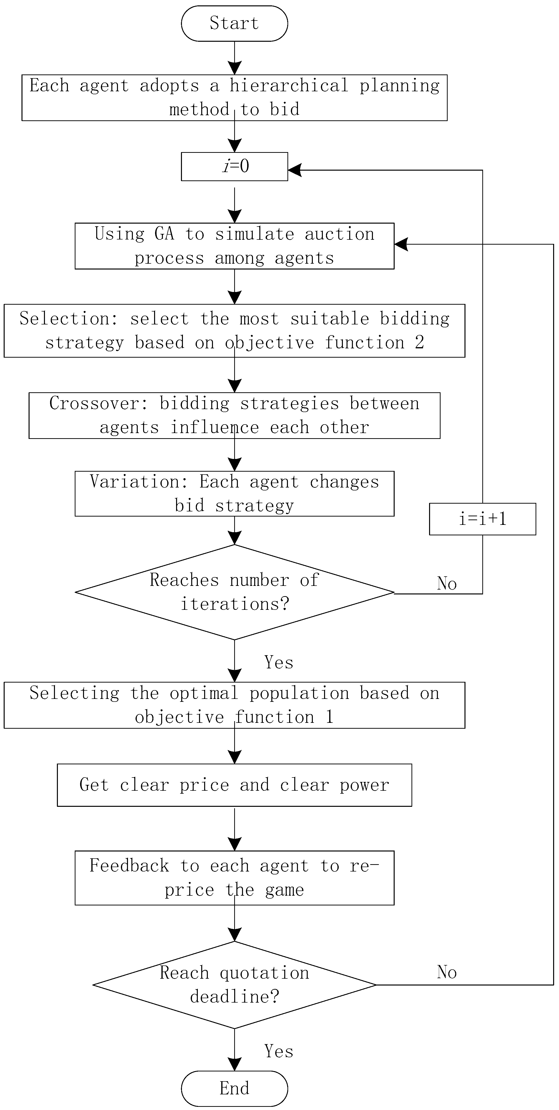
3.3.2. Dynamic Game Process

The calculation of this model includes two parts. The first part is the game competition among multi-agents. The second part is the dynamic game between VPP agents and trading centers. GA is used to simulate the process of mutual bidding between multiple agents. For the two objective functions of the bidding process, the hierarchical planning method is used for analysis [35]. The processes of selection, crossover, and mutation in GA are similar to the bidding rules between agents. In the process of selection, the optimal bidding strategy is based on the maximum revenue of each agent (Objective Function 1). That is, in the process of bidding, each agency tends to have a bidding strategy that maximizes the agency’s own revenue. In the crossover process, the bid prices between the agents affect each other, and the agents change their own quotes according to the historical quote information of other agents. In the process of variation, in connection with the actual situation, the bids of each agency cannot be kept in good order, and they will suddenly reduce or raise the bid price according to their own situation and information, but the bid price will also be within a certain range. Using GA to simulate the bidding game process is a simulation scheme under the premise of following the actual situation of each agent and the electricity market. After the bidding process is over, the optimal solution is selected according to the maximum social benefit (Objective Function 2) in the population, that is, the optimal bidding scheme. The process is shown in Figure 5.

4. Case Study

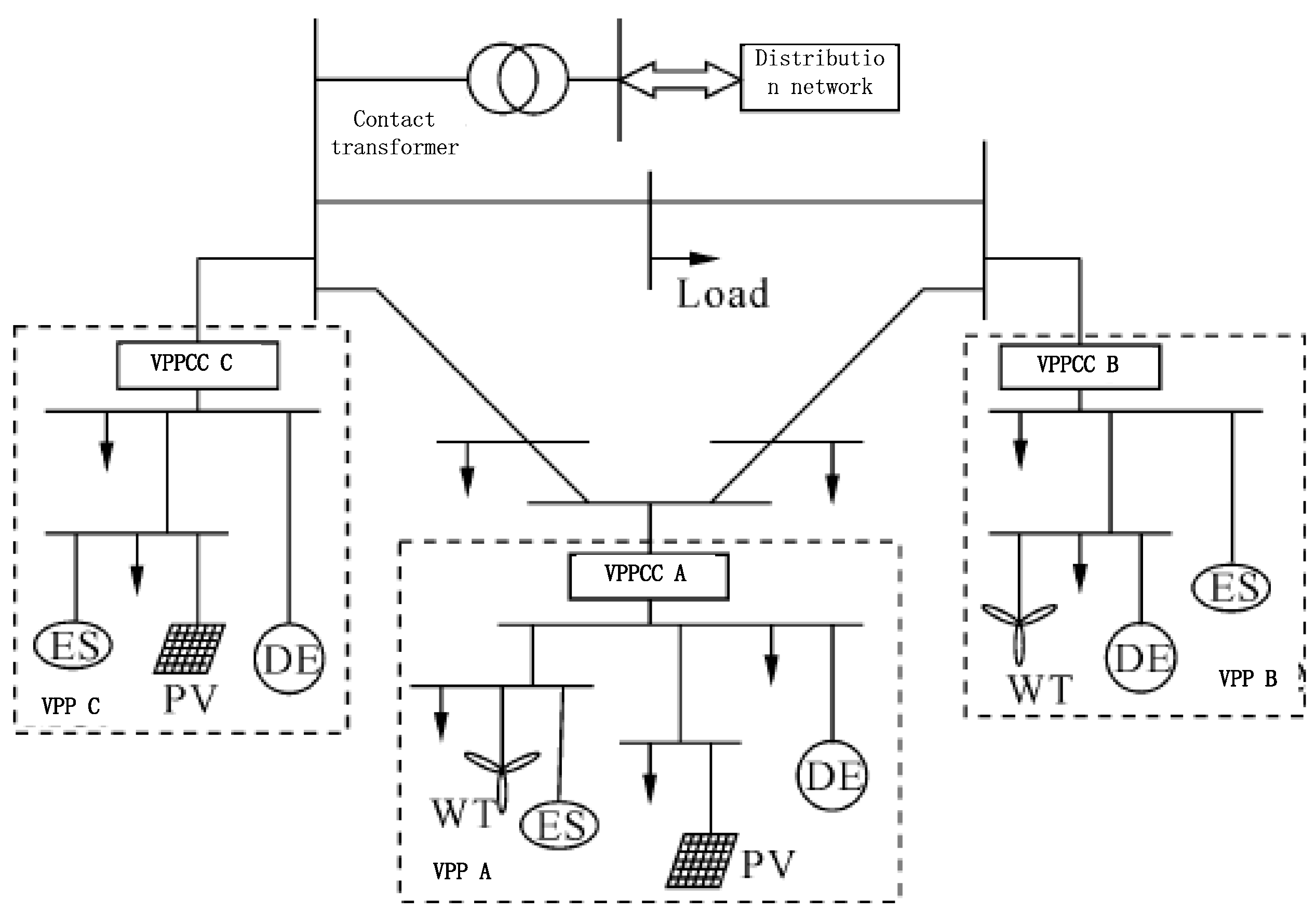
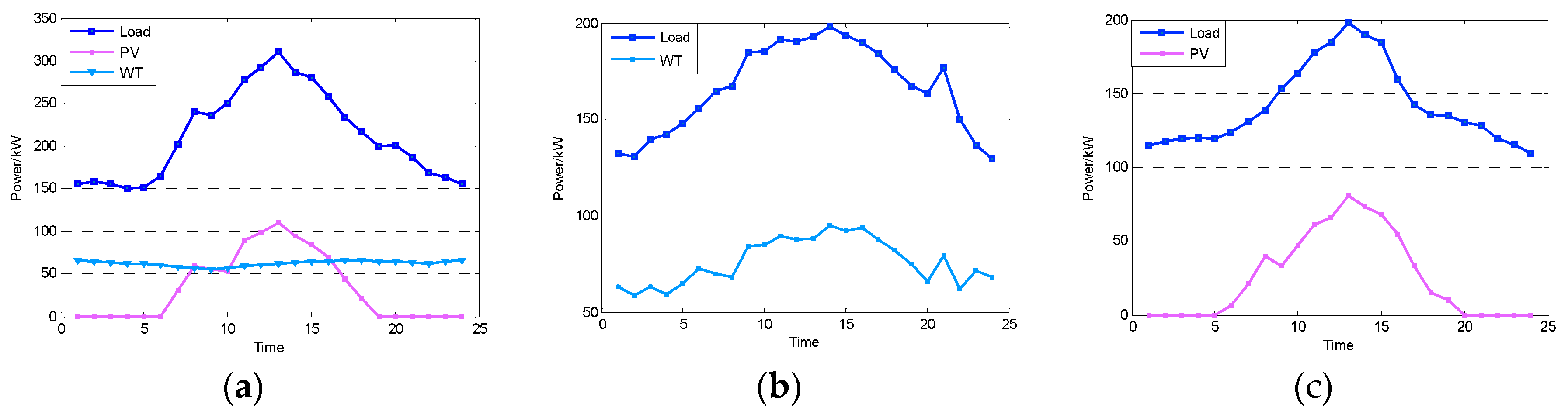
4.1. Case Description

An IEEE-9 node system with three VPPs was adopted for case verification, as shown in Figure 6. Line parameters can be found in [36]. The VPP Center Controller (VPPCC) is a monitoring and management unit that bears the functions of communication, monitoring, and management with various devices. To reflect the differences between different VPPs, VPP A consists of DE1, WT1, PV1, and ES1. VPP B consists of DE2, WT2, and ES2. VPP C consists of DE3, PV3, and ES3. The specific parameters are shown in

Table 1. DE and ES parameter settings in VPP.

Type	Rated Capacity/kW			Maximum Power/kW			Minimum Power/kW			Cost/(¥/kW)
	VPPA	VPPB	VPPC	VPPA	VPPB	VPPC	VPPA	VPPB	VPPC
DE	180	120	180	180	120	180				0.56
ES	100	60	60	65	38	38	−15	−15	−15	0.98

.

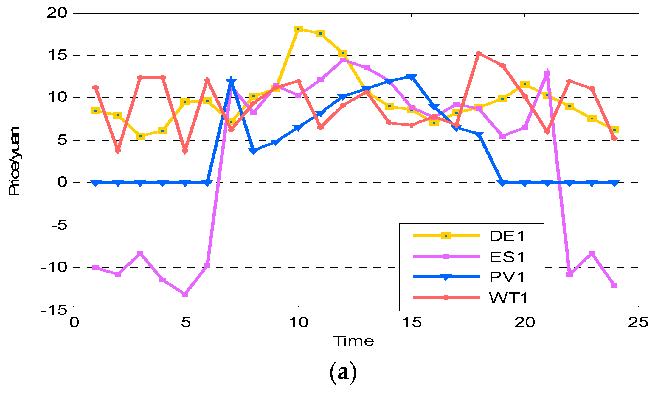
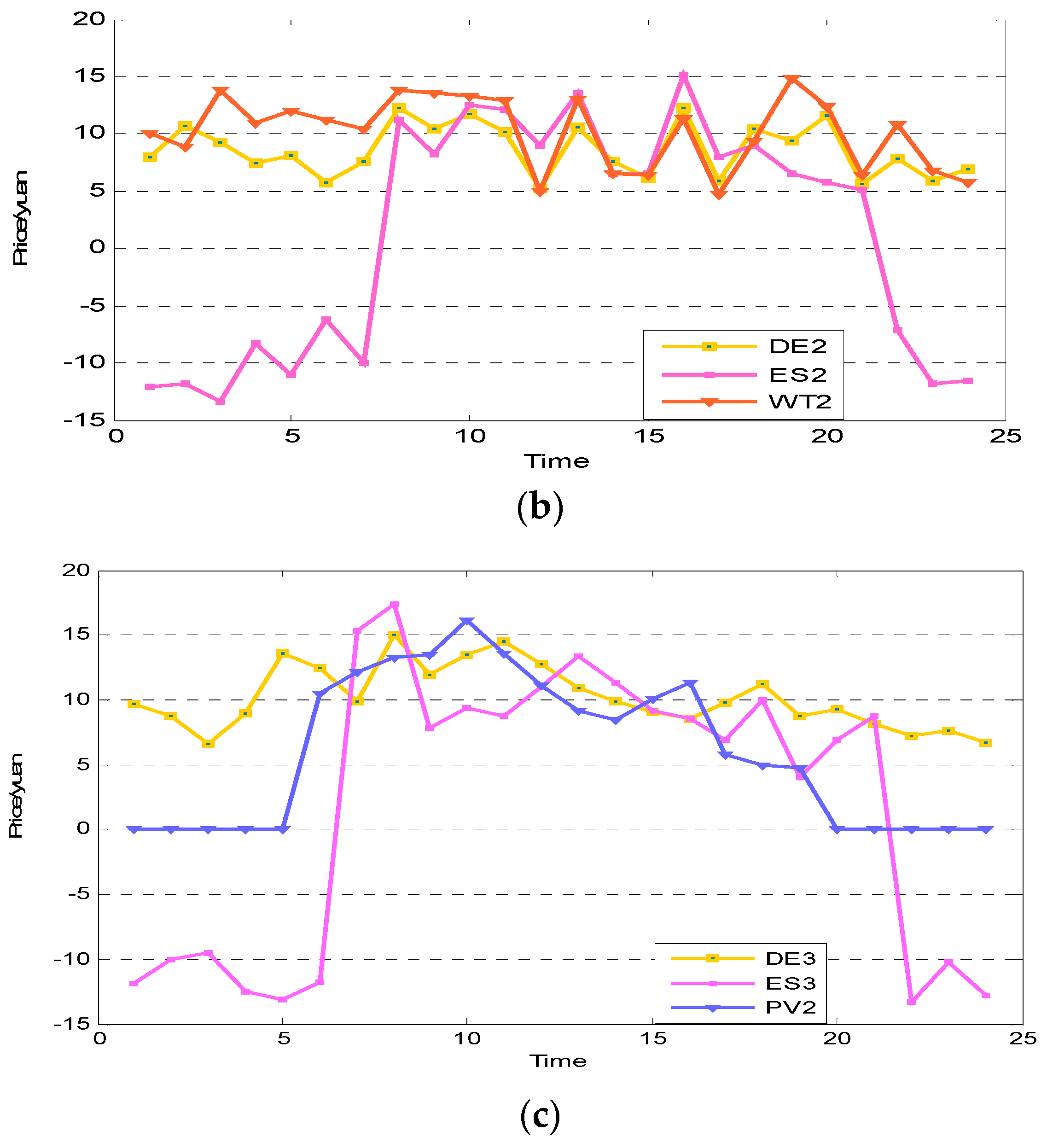
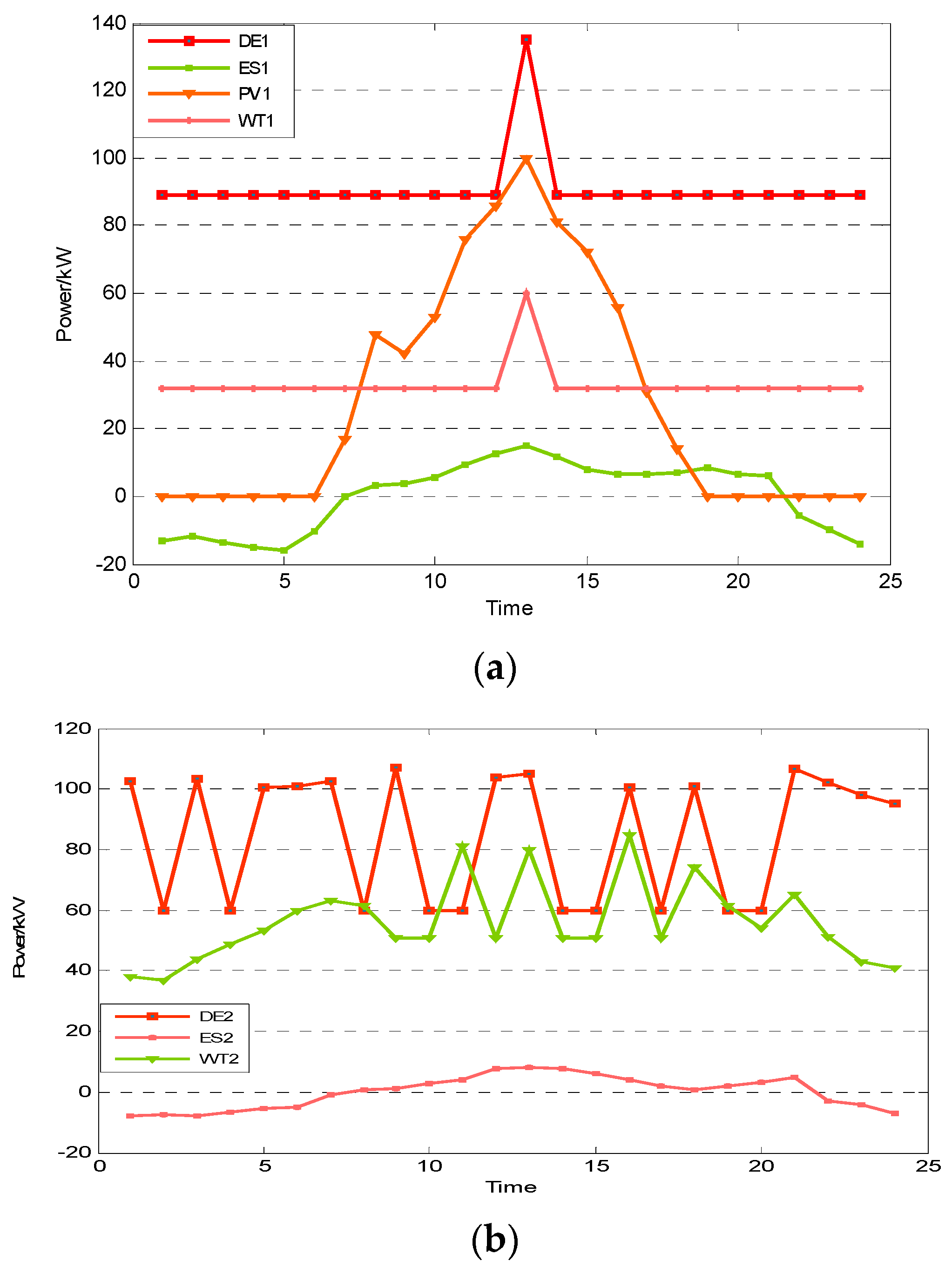
4.2. VPP Internal Bidding Results

The normal distribution model of the load prediction error expects μ_L = 0.02. The PV prediction model expects μ_PV = 0.07 (sunny, error is ND). The wind power prediction model expects μ_WG = 0.05 (wind speed interval is 5.1–9.8, error is ND). The model of TL load transfer rate expects μ_TL,I = 0.5, μ_TL,O = 0.7554. The model expects of the ES charge and discharge motion parameters is μ_ES = 0.8, and the standard deviation of all models is σ = 0.2. Using Monte Carlo simulation (MCS) to generate electricity price data, C_TL takes the average price of electricity. Β = −1.3, η_ch = η_dis = 0.85, λ₀ = 0.8, a_ch = −0.8327, b_ch = 0.6255, a_dis = 1.5895, b_dis = 0, T_f = 9:00–22:00, T_g = 1:00–8:00 and 23:00–24:00. Figure 7 shows the load and DER prediction results for the three VPPs.

Using Matlab software to program and run the model and algorithm, the dynamic game results of the internal market operation of VPP can be obtained. Taking VPP A as an example, Figure 8 shows the dynamic process of each subagent’s bidding strategies in the market as the game times N increases in a certain period. In Figure 8, it can be seen that, after repeated games, the subagents obtain equilibrium solutions after about 200 rounds.

The process shown in Figure 3 was used to solve the model.

Table 2. Subagent quotations, winning bids, and market clearing prices at a certain time within VPP.

		Quotation/¥	Winning Bids/kW	Profit/¥	Clearing Price/¥
VPPA	DE1	10.68	135	513	10.68
	ES1	13.60	15	6
	PV1	11.11	100	200
	WT1	10.72	60	84
VPPB	DE2	10.88	105	375	10.88
	ES2	13.56	8	14
	WT2	12.59	80	171
VPPC	DE3	11.01	115	449	10.59
	ES3	13.35	8	10
	PV2	10.59	75	209

only lists the quotations, the electricity quantity of acceptance of the bid, and market clearing prices for each subagent within the three VPPs at a given period. Assume that three VPPs participate in the day-ahead market bidding. The clearing electricity quantities obtained at the corresponding time are 310, 193, and 198 kW, respectively. Figure 9 shows the sub-agency quotes for each of the three VPP’s internal day markets in 24 periods, while Figure 10 shows the winning bids for each subagent during per period.

As can be seen from the quotations and market clearances of the three subagents within the VPP, the subagents’ winning power curves are significantly different. VPP A has WT and PV at the same time, and it supplies power to the extra when a low load at night and a large surplus of photovoltaic power at noon. VPP B has wind power WT, so contributes surplus power at night. VPP C, which has PV, contributes the remaining power at noon. Renewable energy sources have greater volatility. At noon, the PV generation power is relatively large. ES absorbs the remaining power for charging and discharges the power at peak load. When the ES device absorbs power, it appears to be in the form of power purchase. Therefore, the quote is negative. When the energy is released, the external device shows the form of power sales. The quotation is positive.

According to Figure 9 and Figure 10, analysis shows that, when it is noon (more PV power) or nighttime (more WT power), renewable energy power generation remains surplus, and sales are prioritized. Therefore, the auction prices of various subagents are generally low. Because WT has windy period (22:00–1:00) at night, WT 2 adopts a relatively low bidding strategy. For PV 2 with a large amount of PV residual power, there is no need to adopt such a strategy. There was larger load at noon (11:00–15:00) and PV power could be effectively consumed. At the same time, the overall bidding strategies tend to have a time-shared price, with a higher peak-loading period and a generally lower grain-loading rate.

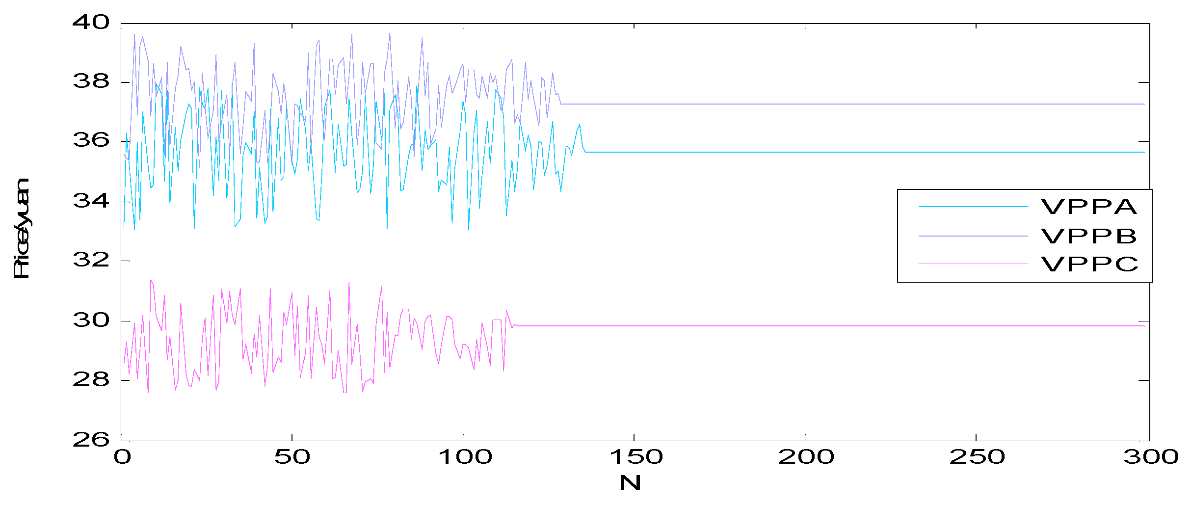
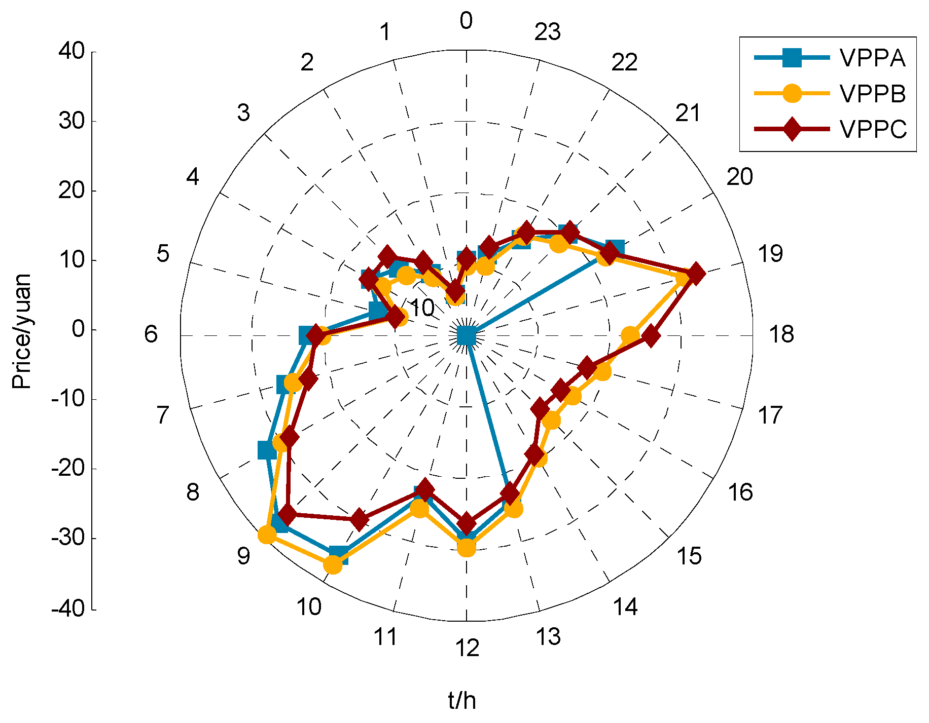
4.3. Auction Result of VPP in the Day-Ahead Market

The analysis of multi-VPP bidding game model is based on the dynamic game model of subagents of VPP in lower layer. Using the Matlab software to program and run the model and algorithm, the dynamic game results of the day-ahead market operation of the power system with multiple VPPs can be obtained. The number of GA iterations is set to 50, the population size is 100, the crossover probability is set to 0.6, the mutation probability is 0.1, and the variable length is 120. Figure 11 shows the dynamic process of the three VPP agent’s bidding strategies in the market as game times N increases.

The process shown in Figure 4 was used to solve the model. Figure 12 shows the quoted prices of three VPP agents in the daily market for 24 periods, and Figure 13 shows the winning bid conditions for each agent in per period.

In the above figures, there are a few differences between the proxy quotes in each period. During 15:00–20:00, VPP A encounters its own maximum load peak, during which the external supply is 0, thus it does not participate in the market bidding. Considering that VPP B has many wind power sources, it releases more electricity to the outside at night. There are many PV power sources in VPP C, thus there are relatively more efforts in the afternoon. The points in Figure 13 represent the externally available load values of VPP, and the VPP bids from the lowest to the highest order, and the available load is superimposed from the inside to the outside. The points in the figure indicate the value of VPP that can be awarded to the outside during the bidding process. Taking time 13:00 as an example, the blue dots (VPP A), the yellow dots (VPP B), and the red dots (VPP C) are lined up from low to high, which shows that, in the bidding process, VPP A has the lowest price, VPP B has the second, VPP C has the highest price, and the TC prefers to select VPP A. Of the 198 kW demanded load at 13:00, VPP A provides 87.6 kW of total external power, followed by VPP B which provides 43.1 kW of total external power, and the remaining portion is borne by VPP 3.

5. Discussion

With the large-scale grid-connected operation of DG, its characteristics of volatility and intermittent have brought certain negative impact on grid voltage, power quality, and dispatch operation. VPP provides new ideas for the development of new energy by aggregating this type of distributed energy. However, the current research on VPP mainly focuses on the overall external operation mode, and usually ignores the internal distributed energy complementary operation modes and benefits. The research can be divided into two parts. The first part is about the VPP of multi-investment subject. Based on the multi-agent technology and the theory of Stackelberg game, the dynamic game bidding model of VPP internal subagent was constructed. Then, in the second part, referring to the clearing results after each round of internal games, a VPP dynamic game bidding model based on multi-agent technology was established.

6. Conclusions

Through the previous research analysis and argumentation, the main conclusions of this paper can be summarized as follows.

Firstly, based on a brief overview of the basic components of VPP, the uncertainties of photovoltaic power generation, wind power generation, and demand-side response within VPP were modeled separately.

Secondly, regarding DER as a subagent of VPP, a subagent’s bidding model in VPP internal market based on dynamic game theory was established. The MCS was used to determine the price coefficient of each subagent, and, after repeated games determining its own optimal price and affecting the power system’s day-ahead market clearing, an optimal equilibrium solution was obtained.

Finally, based on the completion of each round of VPP internal market clearing, with reference to the outcome of each round of clearing, a bidding strategy for VPP to participate in the day-ahead market was developed. Based on multi-agent technology, a dynamic competitive game model for electricity market with multiple VPPs was established. VPP and traditional thermal power plants were agents. Based on the methods and strategies that each agency may adopt in the market competition, the dynamic game behavior between VPP and trading market was simulated by GA, and a complete game process of bidding was presented. Verified by examples, the model can provide methods for the efficient use of resources in power systems with multiple VPPs.

References

1. Li, P.; Zhang, X.S.; Zhao, B.; Wang, Z.L.; Sun, J.L. Design and mode switching control strategy for multi-microgrid multi-grid point structure microgrid. Power Syst. Autom. 2015, 39, 172–178. [Google Scholar]
2. Fang, X.; Yang, Q.; Wang, J.; Yan, W. Coordinated dispatch in multiple cooperative autonomous islanded microgrids. Appl. Energy 2016, 162, 40–48. [Google Scholar] [CrossRef]
3. Xue, M.D.; Zhao, B.; Zhang, X.S.; Jiang, Q.Y. Optimized configuration and evaluation of grid-connected microgrid. Electr. Power Syst. Autom. 2015, 39, 6–13. [Google Scholar]
4. Kardakos, E.G.; Simoglou, C.K.; Bakirtzis, A.G. Optimal offering strategy of a virtual power plant: A stochastic bi-level approach. IEEE Trans. Smart Grid 2016, 7, 794–806. [Google Scholar] [CrossRef]
5. Zhu, J.Q.; Duan, P.; Liu, M.B. Electric power real-time balanced dispatching based on risk and source-net-load bi-level coordination. Proc. CSEE 2015, 35, 3239–3247. [Google Scholar]
6. Zhou, Y.Y.; Yang, L. Synergetic scheduling model based on classical scene sets for virtual water power plants. Power Syst. Technol. 2015, 39, 1855–1859. [Google Scholar]
7. Niu, W.J.; Li, Y.; Wang, B.B. Demand-responsive virtual power plant modeling considering uncertainties. Proc. CSEE 2014, 34, 3630–3637. [Google Scholar]
8. Sun, S.; Yang, Q.; Yan, W. A novel Markov-based temporal-SoC analysis for characterizing PEV charging demand. IEEE Trans. Ind. Inform. 2018, 14, 156–166. [Google Scholar] [CrossRef]
9. Zhao, H.; Wu, Q.; Hu, S.; Xu, H.; Rasmussen, C.N. Review of energy storage system for wind power integration support. Appl. Energy 2015, 137, 545–553. [Google Scholar] [CrossRef] [Green Version]
10. Liu, Y.Y.; Jiang, C.W.; Tan, S.M.; Hu, J.Z.; Li, Q.S. Optimal scheduling strategy of virtual power plant considering risk-adjusted threshold of capital yield. Proc. CSEE 2016, 36, 4617–4627. [Google Scholar]
11. Zamani, A.G.; Zakariazadeh, A.; Jadid, S. Day-ahead resource scheduling of a renewable energy based virtual power plant. Appl. Energy 2016, 169, 324–340. [Google Scholar] [CrossRef]
12. Zang, H.X.; Yu, S.; Wei, Z.N.; Sun, G.Q. Two-layer optimal scheduling of virtual power plant considering safety constraints. Electr. Power Autom. Equip. 2016, 36, 96–102. [Google Scholar]
13. Guo, H.X.; Bai, H.; Liu, L.; Wang, X.L. Virtual power plant optimization scheduling model under uniform energy market. J. China Electrotech. Soc. 2015, 30, 136–145. [Google Scholar]
14. Rahimiyan, M.; Baringo, L. Strategic bidding for a virtual power plant in the day-ahead and real-time markets: A price-taker robust optimization approach. IEEE Trans. Power Syst. 2016, 31, 2676–2687. [Google Scholar] [CrossRef]
15. Mnatsakanyan, A.; Kennedy, S.W. A novel demand response model with an application for a virtual power plant. IEEE Trans. Smart Grid 2015, 6, 230–237. [Google Scholar] [CrossRef]
16. Liu, J.N.; Li, P.; Yang, D.C. Virtual power plant bidding strategy based on combined wind and solar storage optimization. Electr. Power Eng. Technol. 2017, 36, 32–37. [Google Scholar]
17. Song, W.; Wang, J.W.; Zhao, H.B.; Song, X.J.; Li, W. Multi-stage bidding strategy for virtual power plant considering demand-responsive trading market. Power Syst. Prot. Control 2017, 45, 35–45. [Google Scholar]
18. Yang, J.J.; Zhao, J.H.; Wen, F.S.; Xue, Y.S.; Li, L.; Lv, H.H. Competitive bidding strategy for virtual power plants with electric vehicles and wind turbines. Electr. Power Syst. Autom. 2014, 38, 92–102. [Google Scholar]
19. Peik-Herfeh, M.; Seifi, H.; Sheikh-El-Eslami, M.K. Decision making of a virtual power plant under uncertainties for bidding in a day-ahead market using point estimate method. Int. J. Electr. Power Energy Syst. 2013, 44, 88–98. [Google Scholar] [CrossRef]
20. Fang, Y.Q.; Gan, L.; Ai, X.; Fan, S.L.; Cai, Y. Bi-level bidding strategy of virtual power plant based on master-slave game. Electr. Power Syst. Autom. 2017, 41, 61–69. [Google Scholar]
21. Mashhour, E.; Moghaddas-Tafreshi, S.M. Bidding strategy of virtual power plant for participating in energy and spinning reserve markets—Part I: Problem formulation. IEEE Trans. Power Syst. 2011, 26, 949–956. [Google Scholar] [CrossRef]
22. Mashhour, E.; Moghaddas-Tafreshi, S.M. Bidding strategy of virtual power plant for participating in energy and spinning reserve markets—Part II: Numerical Analysis. IEEE Trans. Power Syst. 2011, 26, 957–964. [Google Scholar] [CrossRef]
23. Zhou, Y.Z.; Sun, G.Q.; Huang, W.J.; Xu, Z.; Wei, Z.N.; Chen, S.; Chen, S. Multi-regional virtual power plant integrated energy coordination scheduling optimization model. Proc. CSEE 2017, 37, 6780–6790. [Google Scholar]
24. Yuan, G.L.; Chen, S.L.; Liu, Y.; Fang, F. Economical optimal scheduling of virtual power plants based on time-of-use pricing. Power Syst. Technol. 2016, 40, 826–832. [Google Scholar]
25. Wang, Y.; Ai, X.; Tan, Z.; Yan, L.; Liu, S. Interactive dispatch modes and bidding strategy of multiple virtual power plants based on demand response and game theory. IEEE Trans. Smart Grid 2016, 7, 510–519. [Google Scholar] [CrossRef]
26. Chitsaz, H.; Amjady, N.; Zareipour, H. Wind power forecast using wavelet neural network trained by improved Clonal selection algorithm. Energy Convers. Manag. 2015, 89, 588–598. [Google Scholar] [CrossRef]
27. Wang, S.; Zhang, N.; Wu, L.; Wang, Y. Wind speed forecasting based on the hybrid ensemble empirical mode decomposition and GA-BP neural network method. Renew. Energy 2016, 94, 629–636. [Google Scholar] [CrossRef]
28. Yadav, A.K.; Chandel, S.S. Solar radiation prediction using Artificial Neural Network techniques: A review. Renew. Sustain. Energy Rev. 2014, 33, 772–781. [Google Scholar] [CrossRef]
29. Wei, B.; Suo, Q.; Lin, X.N.; Li, Z.T.; Chen, L.; Deng, K.; Bo, Z.Q.; Huang, J.G.; Muhammad, S.K.; Owolabi, S.A. Daily operation energy control optimization strategy of wind/light/chai/gull islanding microgrid considering transferable load efficiency. Chin. J. Electr. Eng. 2018, 38, 1045–1053. [Google Scholar]
30. Ai, X.; Zhou, S.P.; Zhao, Y.Q. Research on an optimal scheduling model with interruptible load based on scenario analysis. Proc. CSEE 2014, 34, 25–31. [Google Scholar]
31. Prabavathi, M.; Gnanadass, R. Energy bidding strategies for restructured electricity market. Int. J. Electr. Power Energy Syst. 2015, 64, 956–966. [Google Scholar] [CrossRef]
32. Nguyen, D.T.; Le, L.B. Optimal bidding strategy for microgrids considering renewable energy and building thermal dynamics. IEEE Trans. Smart Grid 2014, 5, 1608–1620. [Google Scholar] [CrossRef]
33. Wu, S.P.; Hu, Z.C.; Song, Y.H. Optimal configuration method of wind farm energy storage combining stochastic programming and sequential monte carlo simulation. Power Syst. Technol. 2018, 42, 1055–1062. [Google Scholar]
34. Zhu, Q.L.; Ma, X.S.; Yuan, J.S. Uncertainty planning method of power generation companies’ competitive bidding strategies considering transmission capacity constraints. J. China Electrotech. Soc. 2012, 27, 216–223. [Google Scholar]
35. Zhang, L.; Jin, Z.D. Research on hierarchical planning method of distribution network based on particle swarm optimization. Shaanxi Electr. Power 2014, 42, 44–47. [Google Scholar]
36. Feng, Y.; Qi, Z.J.; Zhou, Q.; Sun, J.W. Online risk assessment and prevention control considering wind power access. Electr. Power Autom. Equip. 2017, 37, 61–68. [Google Scholar]
Figure 1. VPP model diagram.
Energies 11 03072 g001
Figure 2. Framework diagram of a double-layer dynamic game model based on multi-agent technology.
Energies 11 03072 g002
Figure 3. VPP internal market bidding flow chart.
Energies 11 03072 g003
Figure 4. Consumer surplus and producer surplus [34].
Energies 11 03072 g004
Figure 5. Multi-VPP external electricity market bidding flow chart.
Energies 11 03072 g005
Figure 6. Multi-VPP system based on IEEE-9.
Energies 11 03072 g006
Figure 7. VPP internal load and DER forecast results: (a) VPP A; (b) VPP B; (c) VPP C.
Energies 11 03072 g007
Figure 8. Dynamic game process of quoting strategies for subagents within VPPA.
Energies 11 03072 g008
Figure 9. Price quoted by subagents in the VPP internal market: (a) VPP A; (b) VPP B; (c) VPP C.
Energies 11 03072 g009aEnergies 11 03072 g009b
Figure 10. Electricity quantity of winning bids for each subagent in VPP internal market: (a) VPP A; (b) VPP B; (c) VPP C.
Energies 11 03072 g010aEnergies 11 03072 g010b
Figure 11. Dynamic game process of agents’ quotation strategies.
Energies 11 03072 g011
Figure 12. Price quotes for each agent in per period.
Energies 11 03072 g012
Figure 13. Neutral power of each agent during per period.
Energies 11 03072 g013