A High-Efficiency Bidirectional Active Balance for Electric Vehicle Battery Packs Based on Model Predictive Control


1
School of Mechanical Science and Engineering, Jilin University, Changchun 130022, China
2
State Key Laboratory of Automotive Simulation and Control, Jilin University, Changchun 130022, China
3
Zhengzhou Yutong Bus Co., Ltd., Zhengzhou 450016, China
*
Author to whom correspondence should be addressed.
Energies 2018, 11(11), 3220; https://doi.org/10.3390/en11113220
Submission received: 28 October 2018
/
Revised: 14 November 2018
/
Accepted: 15 November 2018
/
Published: 20 November 2018
(This article belongs to the Special Issue Intelligent Control in Energy Systems)
Abstract
:This study designs an active equilibrium control strategy based on model predictive control (MPC) for series battery packs. To shorten equalisation time and reduce unnecessary energy consumption, bidirectional active equalisation is modelled and analysed, and the model predictive control algorithm is then applied to the established state space equation. The optimisation problem that minimises the equilibrium time is transformed to a linear programming form in each cycle. By solving the linear programming problem online, a group of control optimal solutions is found and the series equalisation problem is decoupled. The equalisation time is shortened by dynamically adjusting the equalisation current. Simulation results show that the MPC algorithm can avoid unnecessary energy transfer and shorten equalisation time. The bench experimental result shows that the equilibrium time is reduced by 31%, verifying the rationality of the MPC strategy.
1. Introduction
With the development of the automobile industry, energy conservation and environmental protection technologies have become widespread concerns. Traditional internal combustion engine cars can no longer adapt to the development of the future automobile industry because of their low energy efficiency and exhaust emission pollution, while batteries and electrochemical capacitors have low-cost and environmentally friendly performance features [1,2]. In this situation, new energy vehicles have become the focus of global automotive companies and research institutions [3]. As the main form of new energy vehicles, electric vehicles have received widespread attention. As a means of transport, electric vehicles use electric power instead of fossil fuel to work and generate truly zero emissions and pollution [4,5]. At the same time, lithium cells have become major power cells because of their high energy density and current charge and discharge characteristics [6,7,8]. In addition, the self-discharge rate of these batteries is small, and they have a long service life. To meet the power demand, the voltage of battery pack is approximately several hundred volts [9,10,11,12]. For a long driving range, the total capacity is approximately 100 Kwh. A single battery cell would be insufficient, so hundreds/thousands of cells must be combined as a battery pack for use. The problem is that battery cells can vary, despite the use of advanced production processes. That is, each battery is not guaranteed to be exactly the same as another. Filtering the cells before use is possible to ensure that all the cells of the entire battery pack are identical. However, distinct working conditions of the battery cells, such as temperature and current, vary due to the different layouts of battery packs. Variability of cells in a battery packs is inevitable because the internal resistance of each cell in a series battery pack is different [13]. The energy flowing through each cell is distinct, and these discrepancies will increase with use, which will inevitably further increase the inconsistency of the battery cells within the battery pack. If the inconsistency of the battery cells is handled improperly, then certain cells will be fully charged before the others. In such a case, charging should be stopped to protect the strong cells from being overcharged, which will result in other cells being partially charged. Similarly, during discharge, certain cells will run out of energy before others. The process should be stopped to protect the poor cells from over-discharge, which will leave the energy of other cells unused. All in all, this variability of cells will lead to a substantial decrease in the total capacity of the battery pack. Therefore, the battery balance problem is an important task of battery management system, which protects the battery pack and extends battery life [14]. The energy equalisation technology in a Battery Management System (BMS) ensures that the energy in each cell remains identical by discharging the high-energy cells or charging the low-energy cells, reducing voltage or battery difference between the battery cells and keeping it within reasonable range. In this way, the battery pack can be fully charged and discharged, utilising the capacity of the battery pack to the maximum extent without adversely affecting battery life.
Through energy transfer, overcharging or over-discharging of individual cells is avoided, overall performance of a battery pack is improved, and service life of the battery pack is fully enhanced, thereby boosting the performance and cruising range of electric vehicles.
This study designs an active equilibrium control strategy based on model prediction for series battery packs. Section 2 introduces the current equilibrium algorithm and presents is advantages and disadvantages. Section 3 designs a set of equalisation boards using the principle of distributed equalisation. Section 4 introduces the MPC algorithm and applies it on the DC–DC control method. Section 5 verifies the proposed method, and Section 6 summarises the study.
2. Comparison of Series Balance Schemes
Depending on how to deal with the superfluous energy of battery cells, the balance scheme is divided into passive and active [15,16].
2.1. Passive Balance
This type of balance is called passive because the superfluous energy of battery cells is consumed through a bypass resistance. That is, superfluous energy is consumed by generating heat through a shunt resistance to achieve consistency in the cells’ voltage. This method is effective when a battery pack contains only one cell with superfluous power. However, if that cell has low power, then it will cause the rest of the cells to discharge, which will generate substantial heat [17]. This method will critically reduce energy utilisation efficiency. In addition, the heating phenomenon will become severe, which will further cause an imbalance in temperature distribution. Thus, heat management is necessary for a passive balance.
2.2. Active Balance
Figure 1 shows that the capacitor and each cell are connected in parallel through the control of switch circuit. The advantages of this scheme are the number of capacitor is few, the principle is simple and energy transfer efficiency is high. The setup also has disadvantages, such as several control switches are used, heavy noise is generated during operation and the switches have relatively short life. In addition, when the battery scale is large, no batteries can work simultaneously, and the work efficiency of balance is low. Figure 2 presents the second capacitor-type balance scheme. Each pair of adjacent battery cells can transfer energy through the capacitor between them. This scheme uses as many capacitors as the number of cells in series. By controlling a single-pole double-throw switch, parallel switching between capacitors and battery cells can be achieved. However, when the first and last battery monomers need to be balanced, the transfer energy will pass through all capacitors and battery cells, which reduces the balance efficiency [18].
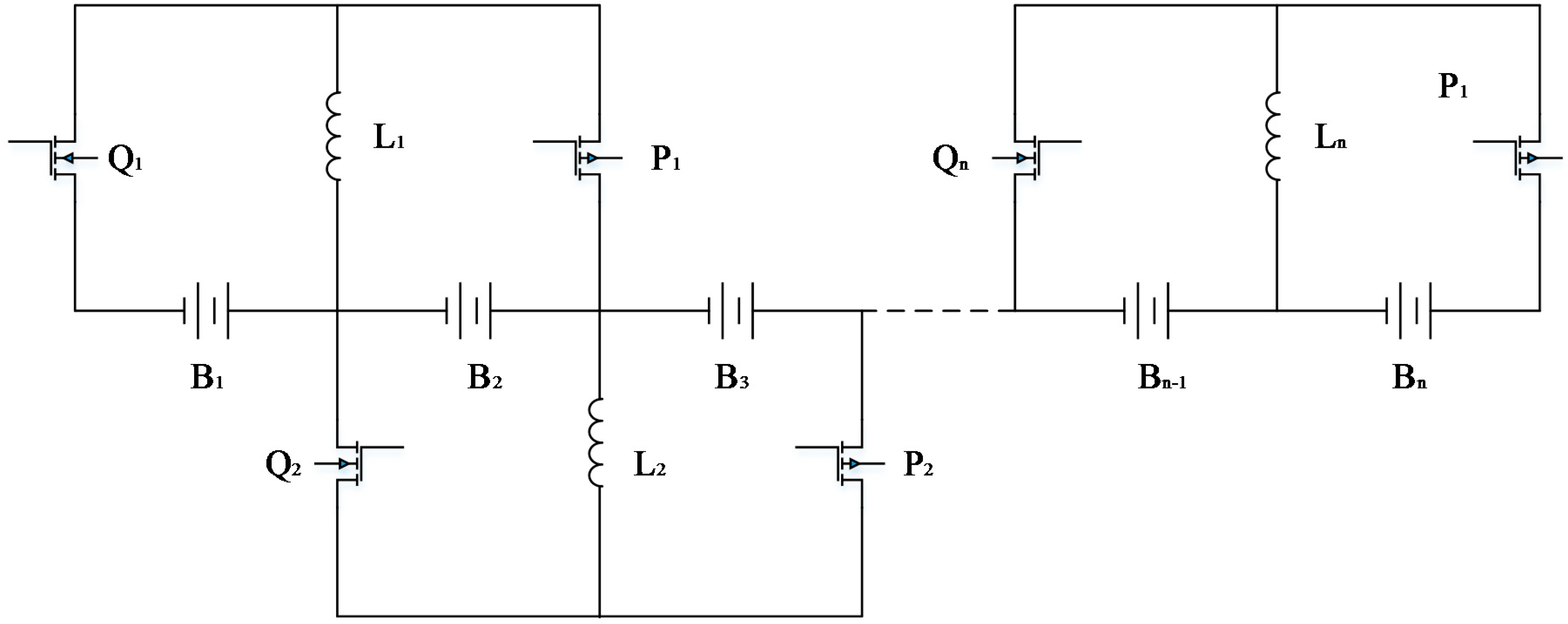
According to the number of inductors, the inductor-type active balance is classified into two types, namely, inductors in the adjacent cells (Figure 3) and an inductor in the battery stack (Figure 4). Figure 3 displays the balance principle of inductors in the adjacent cells. The advantage of this balance method is that it is easy to expand, and the conductor has a high transfer efficiency. However, the electricity transfer between non-adjacent cells will pass through all cells and inductors, which will reduce the efficiency and complicate the control strategy.
Figure 4 illustrates the balance principle of an inductor in a battery stack. The advantage of this balance method is the high-energy transfer efficiency [19]. However, only one balance circuit works at a time, and it is unsuitable for large battery stacks [20].
Figure 5 shows the principle of multi-winding transformer balance [21]. The advantages are its simple control principle and high efficiency, whereas the drawbacks are the high manufacturing requirement of the transformer and unsuitability for expanding the battery pack.
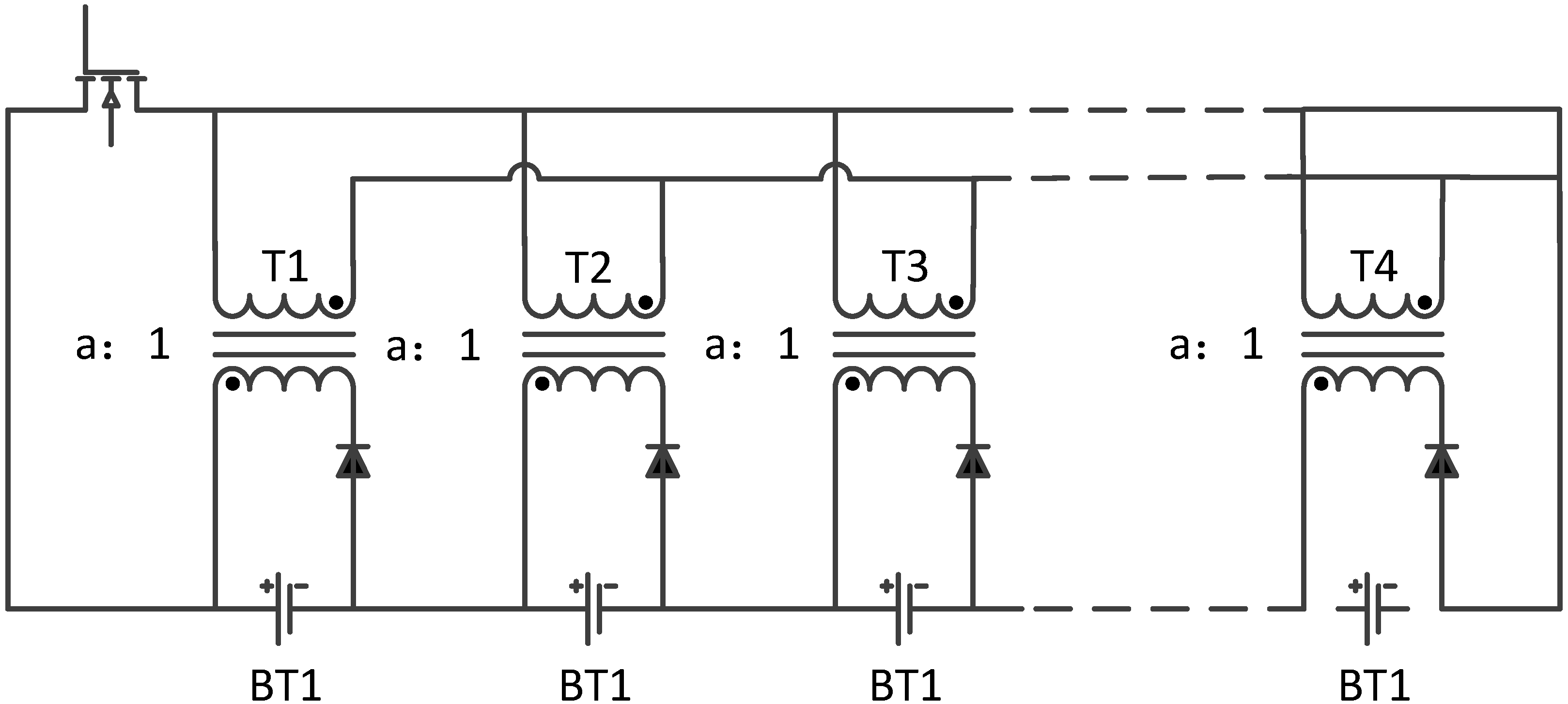
Figure 6 provides the principle of the multi-transformer balance. The expanding the battery pack will be easy [22]. However, the costs for the transformers are high.
Figure 7 demonstrates the principle of the switching transformer balance. The advantage of this balance type is that the energy transfer efficiency is high, but only one balance circuit works at a time and expanding the battery pack is difficult.
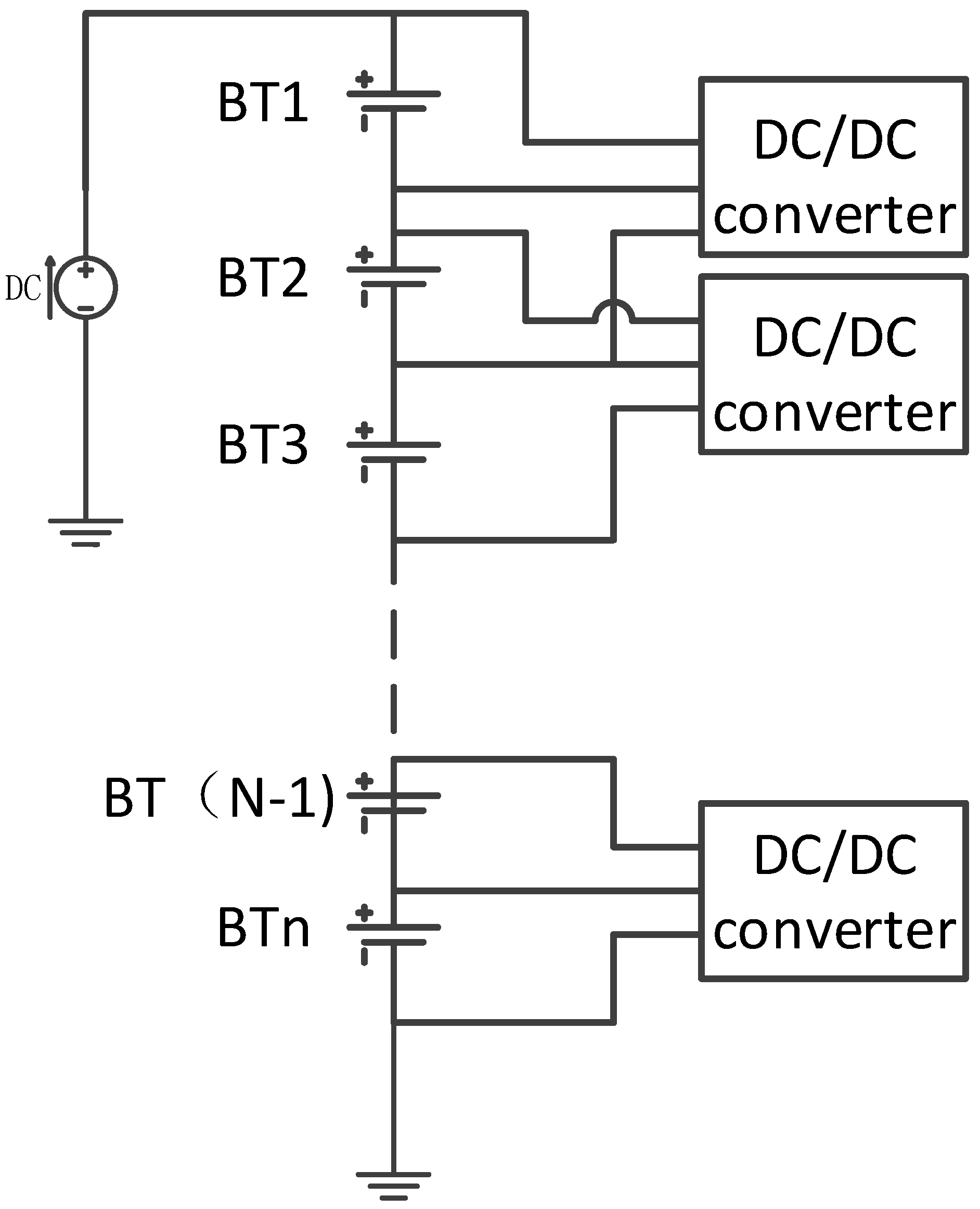
Figure 8 shows the principle of the distributed DC–DC active balance. The electrical energy in this scheme can only be transferred between adjacent cells [23,24]. A large balance current can be achieved due to the high power of the DC–DC module, so this scheme is especially suitable for the internal balance of large capacity cells. However, this scheme also has an obvious disadvantage: the electric energy needs to pass through all battery cells as it is transferred from the top to bottom of the battery stack. This mechanism will reduce balance efficiency.
Figure 9 provides the principle of the centralised DC–DC active balance [25]. The advantages are that the control strategy is flexible and changeable and the power of DC–DC is high. The drawbacks are that the cost of DC–DC is high, and it is unsuitable for large-scale battery stacks.
All in all, passive energy balance is unsuitable for large capacity cells because of its low energy transfer efficiency and long balance time.
In 2011, Kim [20] designed an automatic charge equalization circuit based on regulated voltage source for series connected lithium-ion batteries. In 2015, Shang [26] designed a cell-to-cell battery equalizer with zero-current switching and zero-voltage gap based on quasi-resonant LC converter and boost converter; and Wang [25] designed a novel active equalization method for lithium-ion batteries in electric vehicles. In 2017, Mccurlie [27] studied the fast model predictive control for redistributive lithium-ion battery balancing. For active energy balance, extra energy is difficult to be transferred quickly in the existing technology, and the minimum energy transfer times is not guaranteed [23]. This study designs an active equilibrium control strategy based on model prediction for series battery packs. We focus on the analysis of the energy balance between tandem cells, which rely on fly-back DC–DC to achieve high-efficiency bidirectional active equalisation. Furthermore, we develop a set of BMS, which is suitable for 132 series cells. To shorten equalisation time and reduce unnecessary energy consumption, bidirectional active equalisation is modelled and analysed, and the process is described using state-space equations. Then, the MPC algorithm is applied to the established state-space equations according to the MPC principle. A closed-loop control of the equalisation is established, and a fast MPC algorithm is adopted to equalise the SOC of the battery pack. The optimisation problem that minimised the equilibrium time is transformed into linear programming in each cycle process. By solving the linear programming problem online, a group of control optimal solutions is explored, and the series equalisation problem is decoupled. The first element of the local optimal solutions is applied to the controlled equalisation circuit, and the equalisation time is shortened by dynamically adjusting the equalisation current.
3. Implementation of Bidirectional Active Equilibrium
This section aims to achieve bidirectional active equalisation. Bidirectional active equalisation is realised using a BMS slave controller. However, we need the BMS master controller to send out control commands. For example, the main controller sends out instructions to collect data and analyses the data returned by the slave controller. The slave controller then controls bidirectional active balancing. The BMS master controller is essential to the normal work of the slave controller for bidirectional active equilibrium.
3.1. Function and Principle of BMS Controllers
This study designs an active equalisation circuit that can achieve bidirectional balancing of battery cells and be used in large-scale battery packs. The main functions are:
- (1)
- acquisition of voltage, current and temperature;
- (2)
- protection function;
- (3)
- SOC and SOH estimation function;
- (4)
- equilibrium function.
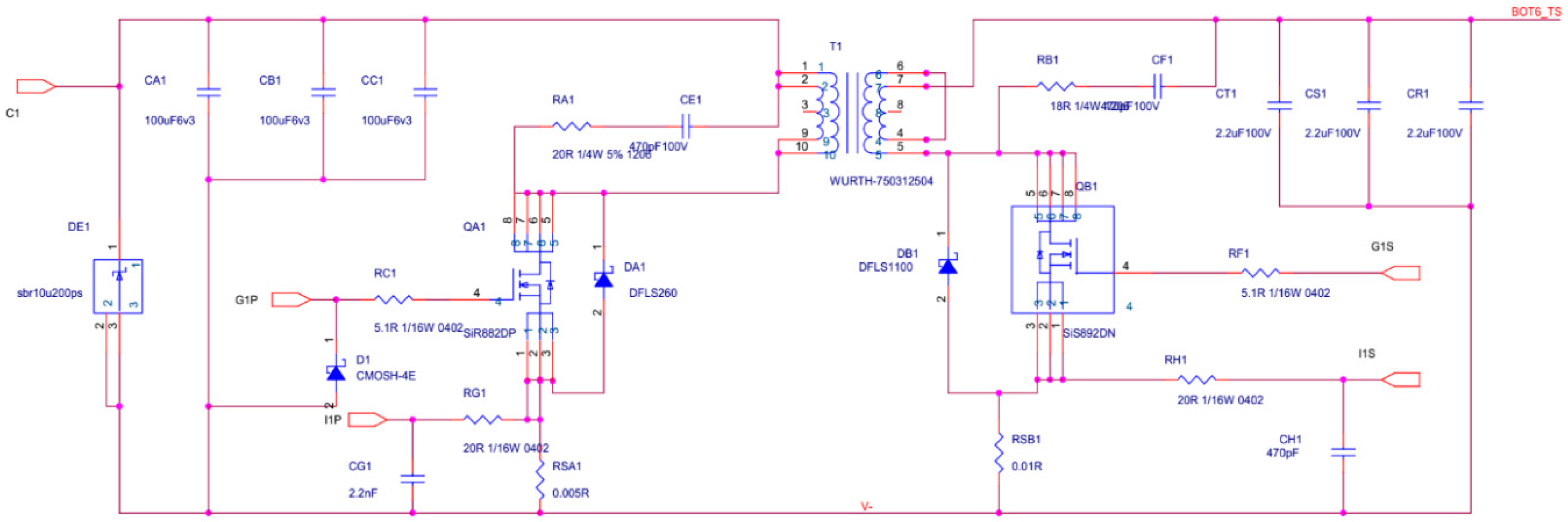
The scheme adopts an improved distributed DC–DC equalisation scheme. Each battery cell is assigned to a DC–DC equaliser, and each equaliser can operate independently. Figure 10 shows the principle underlying the charge transfer between individual cells and a large neighbouring battery stack. The operating principle of the cell discharge is as follows. Taking cell 1 as an example, the switch G1P controls the battery coil to close when cell 1 needs be discharged. Then, cell 1 starts to charge the DC–DC coil (T1), and the magnetic field energy stored in the inductor reaches the maximum value when the charging current reaches the set peak value. During this time, switch G1P is turned off, and the switch G1S is turned on. The energy in the inductor primary winding is transferred to the secondary coil on the side of the battery pack, and the battery module (monitor 1 to battery 12) is charged through switch G1S. When the charging current drops to 0, the G1S is turned off and G1P is turned on synchronously, and cell 1 starts charging the DC–DC again. This process is repeated until the voltage or power of cell 1 recovers to the set level.
The principle of charging the cells is similar to the aforementioned process. Still taking cell 1 as an example, the controller controls the G1S to close when cell 1 needs to be charged. The DC–DC module (T1) firstly takes power from the battery stack (cells 1–12). The energy in the DC–DC module reaches the maximum value when the charging current reaches the maximum value. During this time, G1S is turned off and G1P is closed synchronously. Then, the energy in the DC–DC is converted into electrical energy and begins to charge cell 1. When the charging current drops to 0, G1P is closed again; G1S is turned on synchronously and obtains energy from the battery stack (cells 1–12) again. This process is repeated until the voltage or power of cell 1 recovers to the set level.
3.2. Hardware Design of Bidirectional Active Balance BMS
The main control unit obtains the voltages, current and ambient temperature of the battery pack; and protects the battery pack from being overused, estimates the battery status (SOC, SOH); and communicates with other electronic control units. In this paper, a high-efficiency, low-power 32-bit STM32F446RET is used as the BMS main control unit microprocessor due to the heavy load. Its CPU speed reaches 84 MHz, flash memory reaches 256 bytes, RAM capacity is 64 bytes. It has three USART interfaces, one SDIO interface, three IIC serial bus interfaces, four SPI serial peripheral communication interfaces and one 16-channel 12-bit 2.4MSPS A/D converter. To save the last SOC and SOH values of the battery at the time of power-off, a peripheral 256-byte EEPROM chip is used. Figure 11 presents the main chip and peripheral circuit structure.
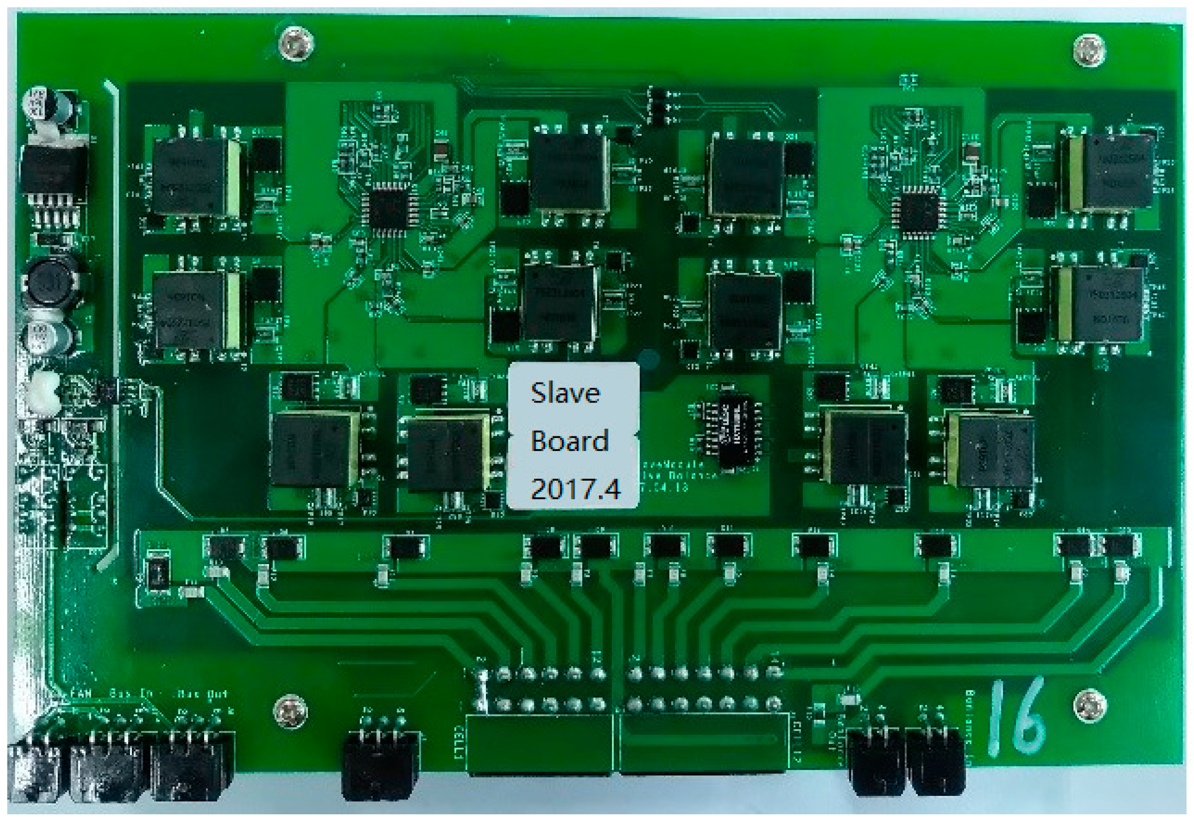
This study adopts Linear Technology’s LTC6804 chip to collect voltage. It is one of the few monitoring chips that can simultaneously collect the voltage of 12 series cells. The measurement error is less than 1.2 mV, and the measurement time of all voltages is less than 290 μs. Therefore, we propose to use this chip to measure the voltage of each battery module with 12 cells. The current of the battery pack is not only an important parameter monitored by the battery protection system but also important information for estimating battery capacity. This study uses a Hall-type current sensor DHAB S/24, which has a dual-range to achieve high accuracy of current acquisition: range 1 is ±75 A, absolute error is ±1.5 A (25 °C). Range 2 is ±500 A with an absolute error of ±5 A (25 °C). This study uses the Bq76PL536 chip to collect the temperature of the main control board; the temperature of cells is collected by the input port of the LTC6804 chip. The balance scheme uses a modular design, in which every 12 cells as a module, and a slave controller to manage the module. One LTC6804 chip is used to read the voltage of 12 cells. Two LTC3300s are used to control the operation of 12 DC–DC to achieve equalisation of individual cells. The protection function is implemented with relays, which employs the EV150-AAD. Figure 12 shows the design of the slave controller, which can achieve a maximum of 4.2 A equalisation current.
The LTC3300’s current acquisition and DC–DC loop traces greatly affect current equalisation. If the current is inaccurate, then it will directly affect the control of the equalisation DC–DC. If the impedance of the DC–DC loop is large, then the equalisation current will be reduced. Therefore, attention should be paid to the route of these lines to maximise the function of the DC–DC module.
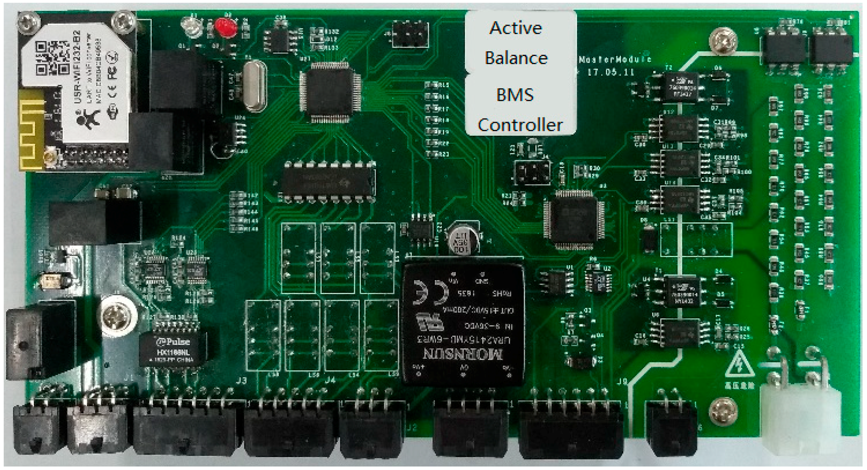
Figure 13 shows the design for the BMS master controller, which communicates with multiple slave controllers through daisy-chain SPI communication technology, controls slave controllers for voltage and temperature acquisition and sends equalisation commands to related slave controllers.
The BMS master controller obtains the cells’ voltages, current and temperature from the slave controllers. Using the information, the master controller protects the cells from overuse, estimates the SOC of the battery and balances the cells if necessary.
3.3. Experiment Results and Analysis
To verify the equalisation effect, we designed an experimental control process, as shown in Figure 14. The monitoring interface communicates with the master controller using the CAN bus, and the master controller communicates with the slave controller using CAT-5 twisted-pair wires.
Figure 15 displays the test bench and the management of a battery pack (containing 132 lithium titanate cells). The process comprises 11 slave controllers, and each one controls 12 cells. The daisy-chain communication is adopted between the slave controllers, and the master controller manages all cells through the lowest-end slave controller.
At the beginning of the experiment, the voltage of the cells in the battery pack is inconsistent. The BMS balances the 132 series cells and collects the voltage of the battery pack. Figure 16 provides the voltages of cells from 1 to 12. The diagram shows that the voltage of cell 1 is gradually pulled up during the equilibrium process. Figure 17 shows the beginning of the equilibrium process, in which the voltage difference among the 12 cells reaches 130 mV. At the end of the process, the maximum voltage difference is controlled within 20 mV, as shown in Figure 18.
4. Model Prediction Control Algorithm
4.1. Basic Principle of Model Prediction Control
Model predictive control (MPC) was developed in the 1970s, mainly due to the requirements of social industrial control and progress in technology, although it is not for control theory. The application for MPC is extensive since its early development. People have turned their attention to MPC methods because they are incapable of building accurate models in complex systems. The MPC algorithm adopts the rolling optimisation concept. In this manner, the requirements of the model accuracy are low, and the amount of real-time calculations is considerably low. Thus, its workload of calculation is less than the traditional optimisation algorithm, and its control effect is moderately well.
Finding a global optimal control variable for a system is difficult for MPC. Fortunately, industrial control does not need such a global optimal control variable as long as a control variable that satisfies the constraint is available in a finitely predicted time domain and makes the cost function locally optimal.
The MPC process can be divided into three steps. Firstly, based on the prediction model and current initial conditions, MPC forecasts the future output within a limited time domain. Secondly, it works out a set of local optimal control variables that can satisfy the constraints of the system and minimise the cost function according to the future model. Thirdly, the first set of control variables in the local control variables obtained during the second step is applied to the controlled system. At the next sampling time, the predictive model is modified based on the actual output value of the system. Then, the process is repeated over and over.
In Figure 19, x0 represents the state of the system in the k moment, u is the system input, y is the system output, Hp is prediction in the time domain and Hc is the control output for the optimal predictive in time domain.
If the model of the controlled system can be expressed by a standard state space model, according to measurement information y(k) and status information x(k), then the predictive model predicts system output in p cycles and solves the optimisation problem, such that the predicted output and set target r in the prediction period have the least errors in the time domain Hp. If the optimal solution to the optimisation problem is control sequence [u(k) u(k + 1) … u(k + c)], then the first element u(k) of the control sequence acts on the controlled object as the current control input and discards other elements.
4.2. Nonlinear Model Predictive Control
Assuming that all state variables of the system are measurable, the problem of nonlinear MPC is described as follows:
where is the state variable of the predictive model, is the system output of the predictive model under control input and is the system output of the predictive model under constraint input.
Actuators have maximum values of output and increments, and their upper and lower limits are constant values. We assume that the controller’s control value, control increments, and output constraints are as follows:
We also assume that the state of the nonlinear system at the current k time can be observed and is ; thus, the discrete model-based optimisation problem can be expressed by the following equation:
If the control and prediction times are hc and cp, respectively, then the constraint in time domain is:
The cost function is:
where Q, R and S are the weighting matrix of the system cost function; is the expected reference output; and is the reference input corresponding to the expected reference output. and are the predicted control and constraint output, respectively, which can be updated using the following equations:
where is the state variable of the system at the current time k, which can be used as the initial condition of the prediction model and starting point for predicting the future output, and is the predictive control input, which takes on the following form:
where and are the independent variables of the cost function. These variables compose vector . The optimal solution for the cost function is :
According to the MPC algorithm, the first component of solution is applied to the system. That is, the current control quantity is
In practical engineering problems, the system’s cost functions and models are often nonlinear. Therefore, the designed controller is typically nonlinear. Solving the optimal solution of the cost function by means of a numerical calculation method is difficult. Furthermore, solving it online is challenging. Scholars use various methods to linearise the problems involved and then employ linear programming to find the optimal solution.
4.3. Optimal Solution for Linear Programming
The linear programming problem is an important part of operations research. Under certain constraint conditions, linear programming guides scholars to find a decision method that has the least cost through mathematical calculation, which highlights the important role of limited resources. Therefore, linear programming problems have widespread applications in various fields, such as path selection, industrial production allocation, business management and so on.
Linear programming problems are divided into two forms. The first form is that of the target function, which has a large output with limited resources. The other one is concerned with achieving the goal with minimum consumption. The former is a maximum value problem, whereas the latter is a minimum value problem. Equations (10) and (11) display the standard form of the linear programming problem model as follows:
The matrix form is shown in the following equations:
where:
In this study, we solve the linear programming problem using MATLAB functions. The steps of the solution are as follows. Firstly, we find a feasible solution using the iterative method, then judge whether it is the optimal solution. If not, then we continue to iterate until an optimal solution is found or determined unsolved.
The following equations show the standard form of linear programming in MATLAB:
The following equations show correlation function, that is:
where lb and ub are the constraint lower and upper limits of the variable x. Conversely, x is the optimal solution of the objective function, Fval is the minimum value of the objective function and exitflag is the state of the solution.
In the MPC for equilibrium, we intend to minimise the equilibrium time. Hence, our cost function can be expressed as:
To convert this problem into a standard linear programming problem, wi and vi can be expressed as in the following equations:
then:
where and .
If:
then, the aforementioned problem can be converted into:
The constraint function can be further expressed as:
In this manner, optimisation can be performed using MATLAB’s linprog() function.
5. Model Predictive Control for Active Equilibrium
Section 3 demonstrates the discharging of the highest voltage battery and charging of the lowest voltage battery. However, if multiple cells need to be balanced simultaneously, then achieving consistency among series cells at a minimum cost (time or energy consumption) is a new problem. We aim to balance all cells in the shortest possible time or with minimal energy loss. Therefore, the goal of battery management system equalisation in general is to select the minimum equilibrium time or energy consumption in equilibrium or a combination of both. To quickly achieve the consistency of the battery and reduce the amount of calculation, this paper chooses the minimum equilibrium time as the objective function of the series equilibrium control. The general control method uses SOC as the equilibrium control condition. That is, the SOC of each battery is compared with the average value. When the SOC of the battery cell is higher than the average value, the battery is discharged, whereas when the SOC of the battery is lower than the average value, the battery needs to be charged. If the equalisation control period is set to a fixed value ΔT, based on the general control method, when a battery needs to be balanced, then it may be charged or discharged for the whole period of ΔT. This leads to the repeated charge and discharge of the battery cell during the entire equilibrium process, which not only reduces the efficiency of the balance but also affects the life of the battery. Based on the MPC method, the MPC controller calculates the equalisation current in each period that is required to complete the equalisation in each cycle based on the difference between the single SOC and average values. The general control method can only calculate whether it needs equalisation but cannot control the magnitude of the equilibrium current. The control of the equalisation current can be realised through PWM. That is, the dynamic adjustment of the equalisation current is achieved by controlling the duty cycle of the equalisation switch in one cycle [28].
5.1. Battery Pack Equalisation Modelling
Suppose the bidirectional DC–DC equalisation system has n series battery in series and m group equalisation channels. The capacity of cell 1 to cell n can be represented by a diagonal matrix based on the metrics outlined in [27,29]. The SOC of each battery is defined as .
The amount of electricity flowing through each string of cells can be expressed as:
where:
The SOC of the battery is a number between 0 and 1, with 0 indicating that the battery power is exhausted and 1 indicating that the battery is fully charged.
If the difference in SOC among cells is large, then energy transfer is needed, and charge is transferred between m channels.
If a diagonal matrix is used to represent the maximum equalisation current of channels 1 to m, the equalisation current of each channel after normalisation is expressed by .
The actual equalisation current can be expressed as:
where:
According to the principle of distributed bidirectional equalisation, which is introduced in the previous section, the electricity discharged from the cell with the highest SOC is transferred to the entire battery pack. If the total transferred electricity is 1, then each cell (including the discharged cell) in the battery pack obtains 1/n of power. Hence 1−1/n electricity is transferred from the discharged cell, and other cells receive 1/n.
Similarly, the battery with the lowest SOC obtains energy from the entire battery pack. If the total transferred electricity is 1, then each cell (including the charged cell) in the battery pack loses 1/n of the energy, such that the charged cell receives 1−1/n of power, and other cells −1/n.
The matrix is used to describe the balanced energy transferred between the cells and indicates the connection between n series of cells and m groups of channels:
The amount of electricity transferred in unit time can be expressed as , where means the battery is being charged, where as means the battery is being discharged.
The goal of equalisation is to realise that the difference between the average value of the SOC and SOC of the cells is less than the threshold value within a short time. That is:
which is close to the target value 0.
If battery capacity x(t) is selected as the state variable, control current u(t) is used as the input control variable and y(t) is the system output variable, then the state control equation of the equalisation can be expressed as
ere A = En, and C = T.
The system constraint is: , that is, a limit is set for the equalisation current of each channel.
5.2. Simulation Experiment Verification
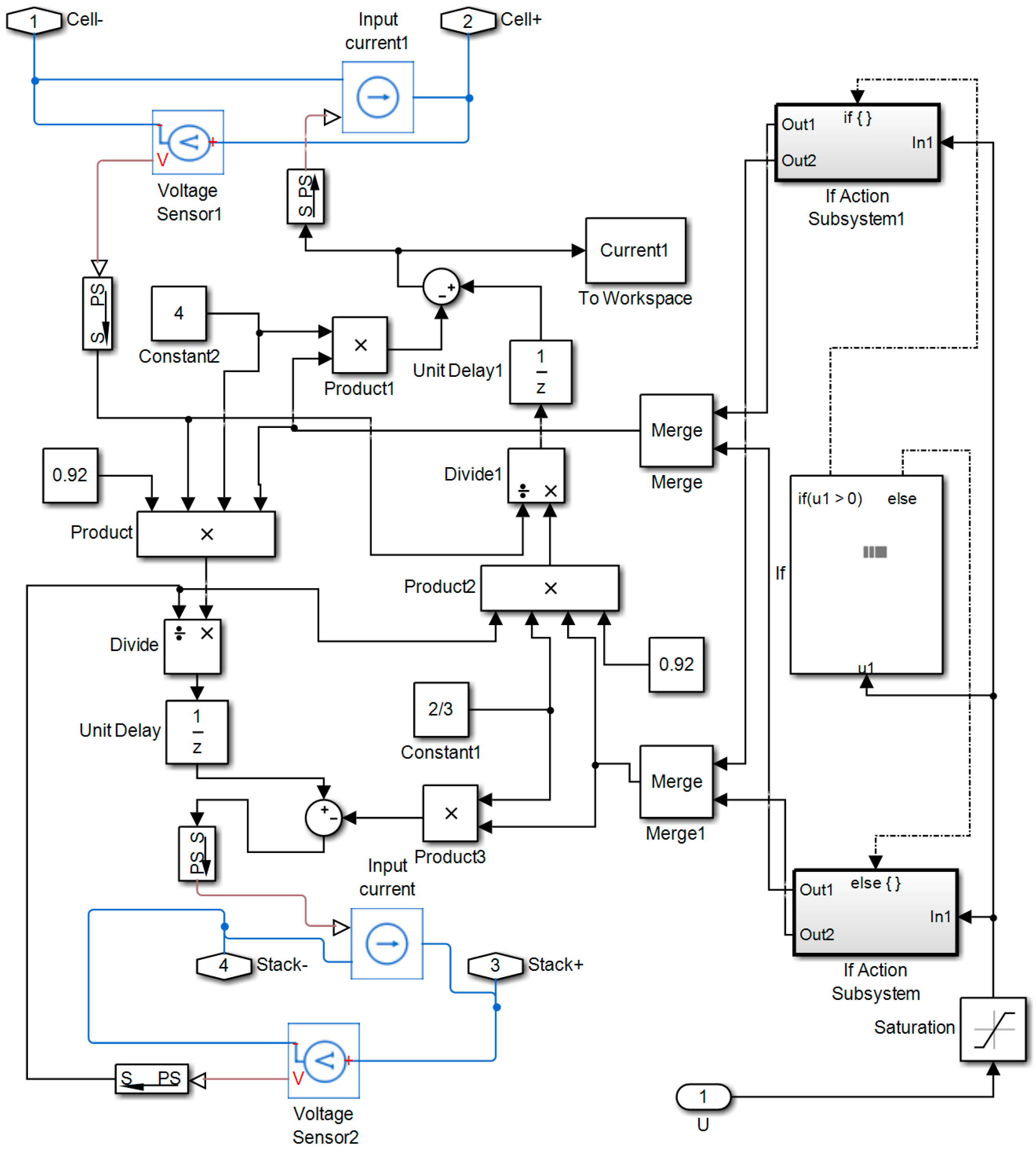
In the previous two sections, the principle of distributed bidirectional DC–DC equilibrium process and model prediction are analysed. In this section, we utilise the battery model in Figure 20 and use Simulink to model the two parts. For simplicity, we select a six-series battery pack for analysis, as shown in Figure 20.
Figure 20 shows that the signal generator in the lower right corner generates the battery pack’s operating current and ambient temperature. The six cells work in series. Each battery has a bidirectional DC–DC equaliser connected to both ends of the cell. The equaliser evens out the cell according to the balanced signal outputted by the MPC controller.
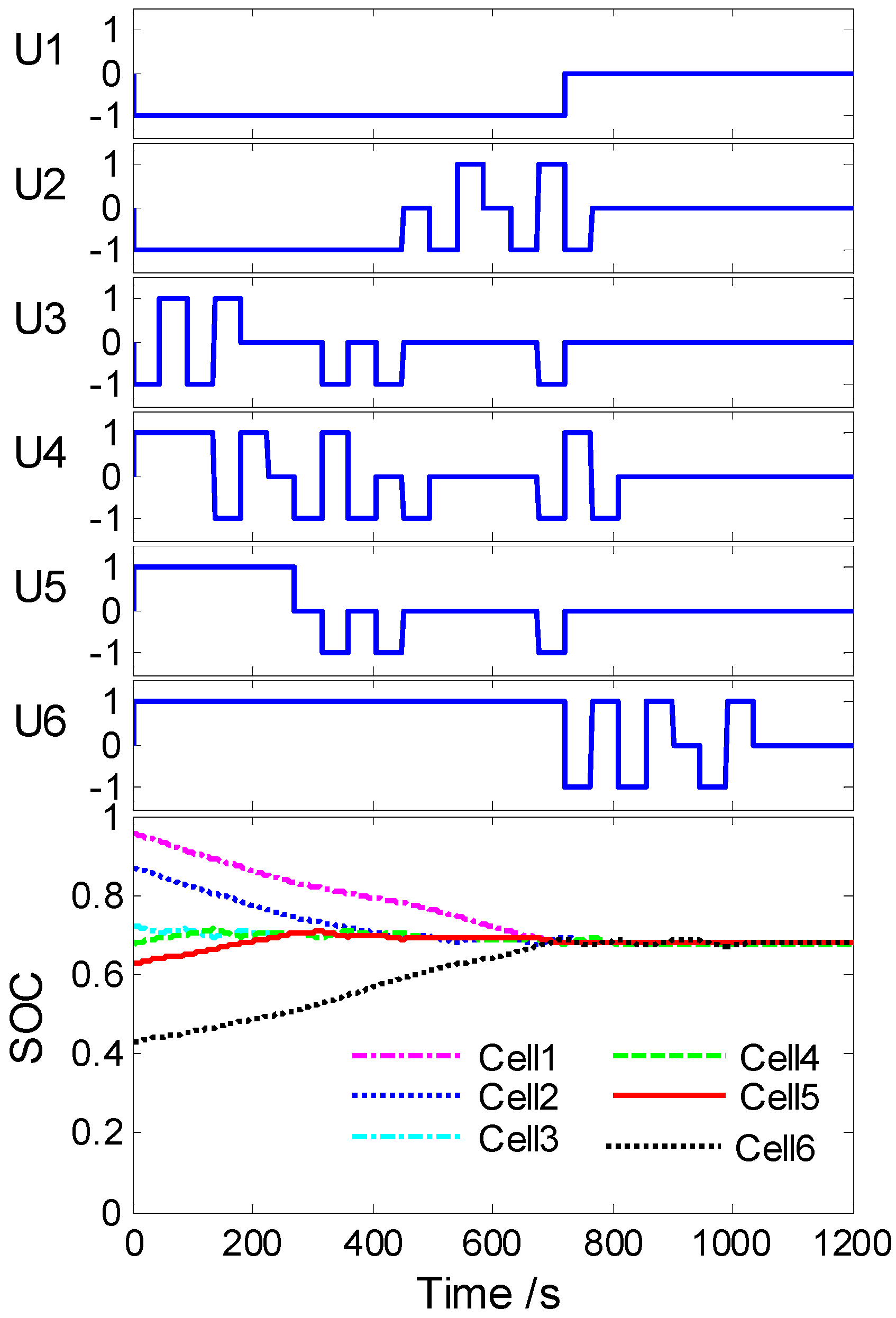
When , the battery is charged, and the charge time in each controller cycle is . Furthermore, when , the battery is discharged, and the discharge time in each controller cycle is . Table 1 shows the initial state of the cells.
Figure 20 further shows that the bidirectional DC–DC is simulated by the model, where ports 1 and 2 are connected to the negative and positive electrodes of the cell, respectively, whereas ports 3 and 4 connect the positive and negative poles of the battery pack ports, respectively. When the battery is charged, the maximum current of the bidirectional DC–DC primary coil (battery side) is 4 A. According to the voltage and current of the battery side, the output power of DC–DC (battery side) can be calculated. Then, according to the conversion efficiency, we can calculate the input power of DC–DC. The output current of the battery pack can be calculated based on the voltage of the battery pack.
Similarly, when the battery is discharged, the DC–DC (battery pack side) input power can be calculated based on the maximum current of the designed DC–DC circuit (battery pack side). Then, through conversion efficiency, the output power of the DC–DC (battery side) can be obtained, then the output current of the battery can be calculated. We set the equalisation control period ΔT = 45 s.
The contrast test adopts SOC as the equilibrium control condition. Based on the general control method, if a battery requires balance, then it may be charged or discharged all the time.
Based on the MPC method, the MPC controller can calculate the equilibrium current in each calculation period based on the difference between single-cell SOC and average value.
The general control method can only calculate the need for equalisation and cannot control the amplitude of the balanced current.
Controlling the equalisation current can be realised by PWM. That is, the dynamic adjustment of the equalisation current is achieved by controlling the duty cycle of the equalisation switch in one cycle. The DC–DC simulation model is shown in Figure 21.
Figure 22 and Figure 23 show the equalisation effect of two equalisation strategies. The two pictures show that these equilibrium strategies can achieve the goal of equilibrium. Compared to the two algorithms, the equalisation circuit is either idle or equalising with the largest balance ability for the common control algorithm in a control cycle. In addition, when a cell is charged, it will discharge the battery that does not need equalisation because electricity is removed from the entire battery pack. As a result of energy loss, they need to be rebalanced, and vice versa. In this manner, battery cells are often charged and discharged repeatedly, which consumes energy, impairs the life of the battery and prolongs equilibration time. By contrast, the MPC algorithm decouples the equalisation and calculates the equalisation current required for each cell to reach a balanced state in every cycle. The required equalising current is then achieved by controlling the duty cycle of the equalising circuit in one control period using the PWM wave. This process avoids repeated charge and discharge of a battery so that the battery pack reaches equilibrium as quickly as possible.
5.3. Bench Test and Result Analysis
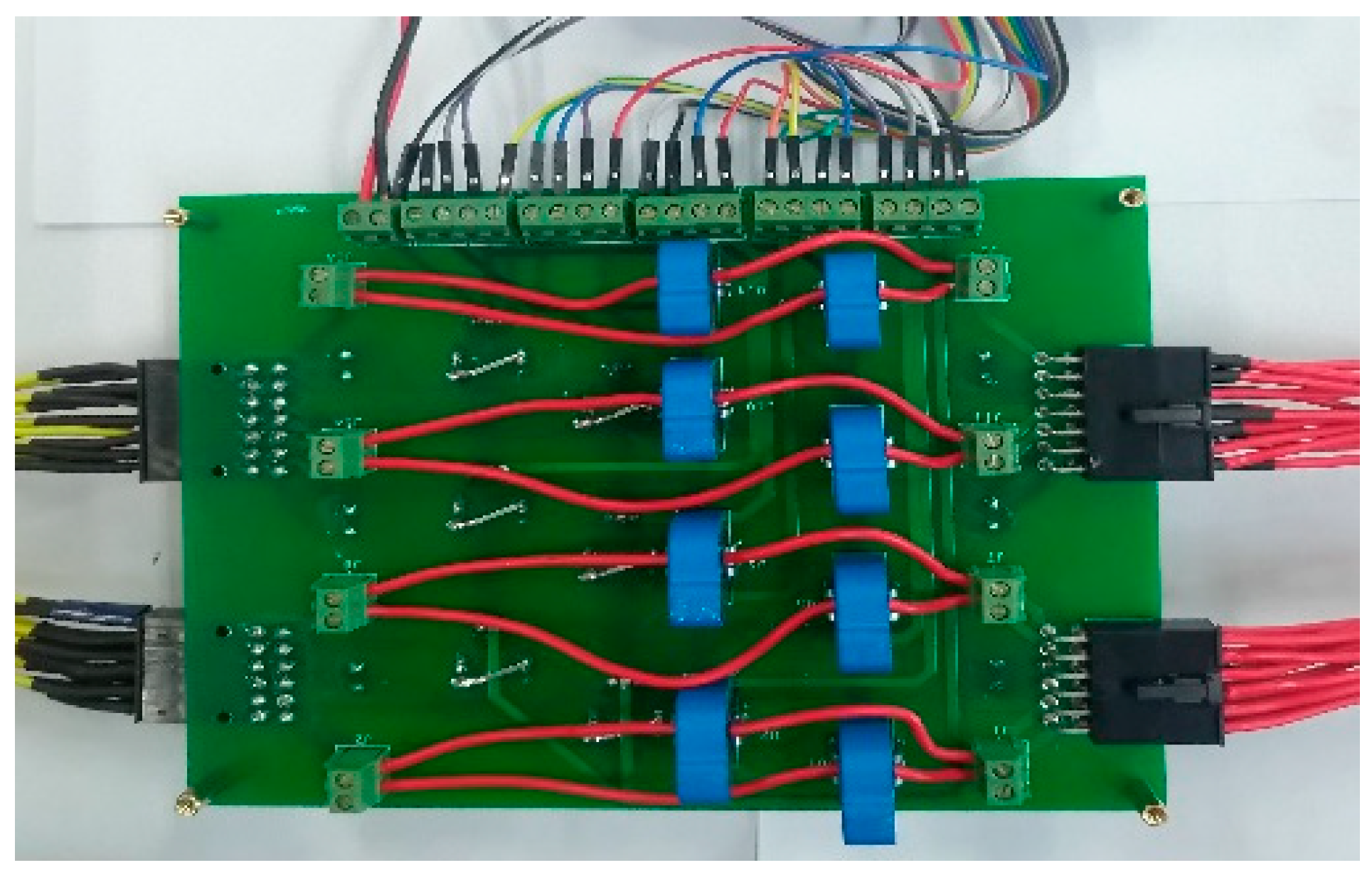
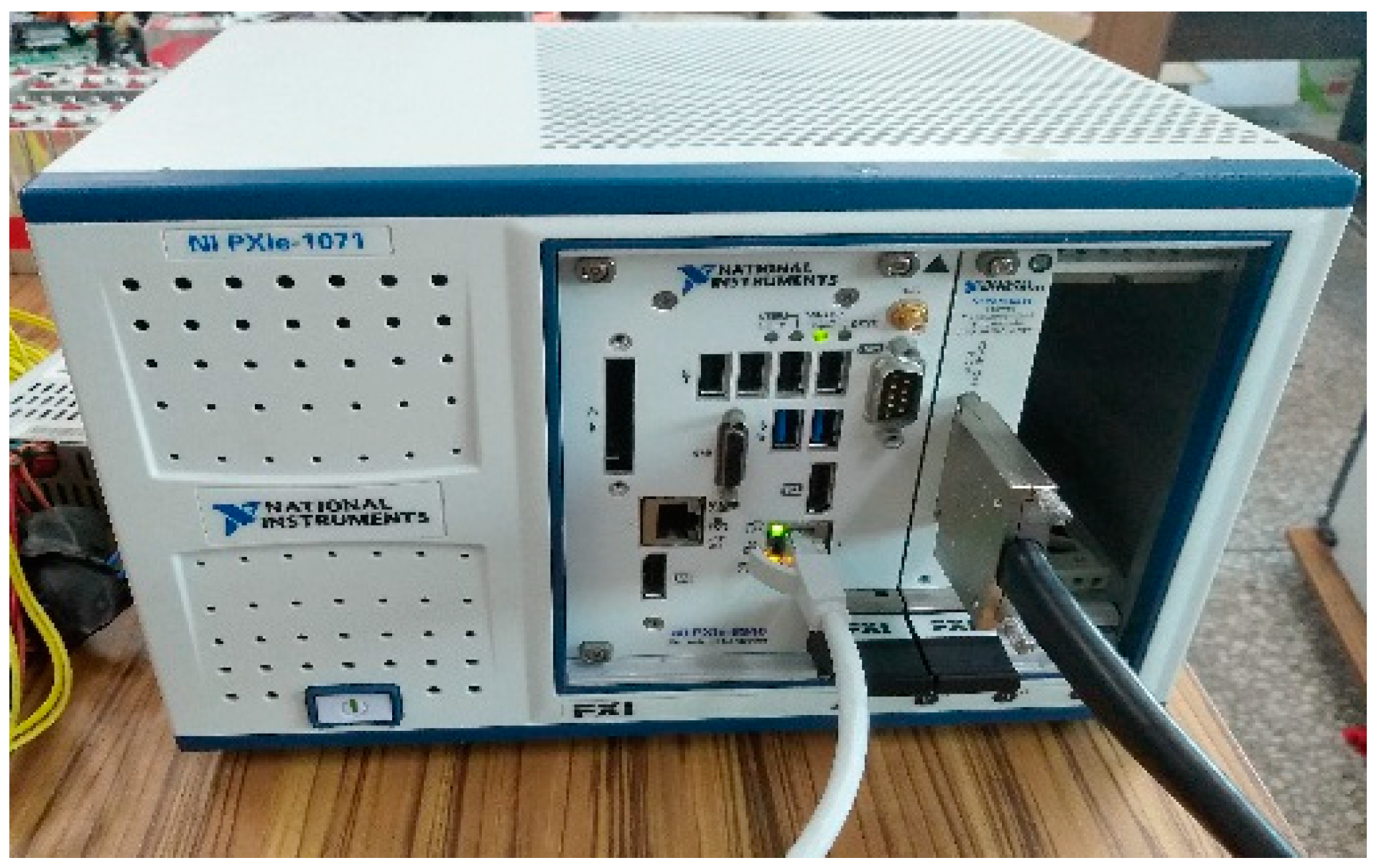
To prove the effectiveness of the proposed control algorithm, this section builds a small battery experimental bench to evaluate the effect of balanced control based on MPC by comparing the collected equalisation current and SOC variation. To measure the equilibrium current of each path, a self-built multi-channel isolated current sensor is used to measure the balanced current, and the NI data acquisition system is used to collect the current sensor output sampling voltage value and convert it into corresponding current value. Battery voltage equalisation and SOC are obtained through the BMS board. Figure 24 presents the 14-channel Hall-type current sensors, whereas Figure 25 displays the NI data acquisition system.
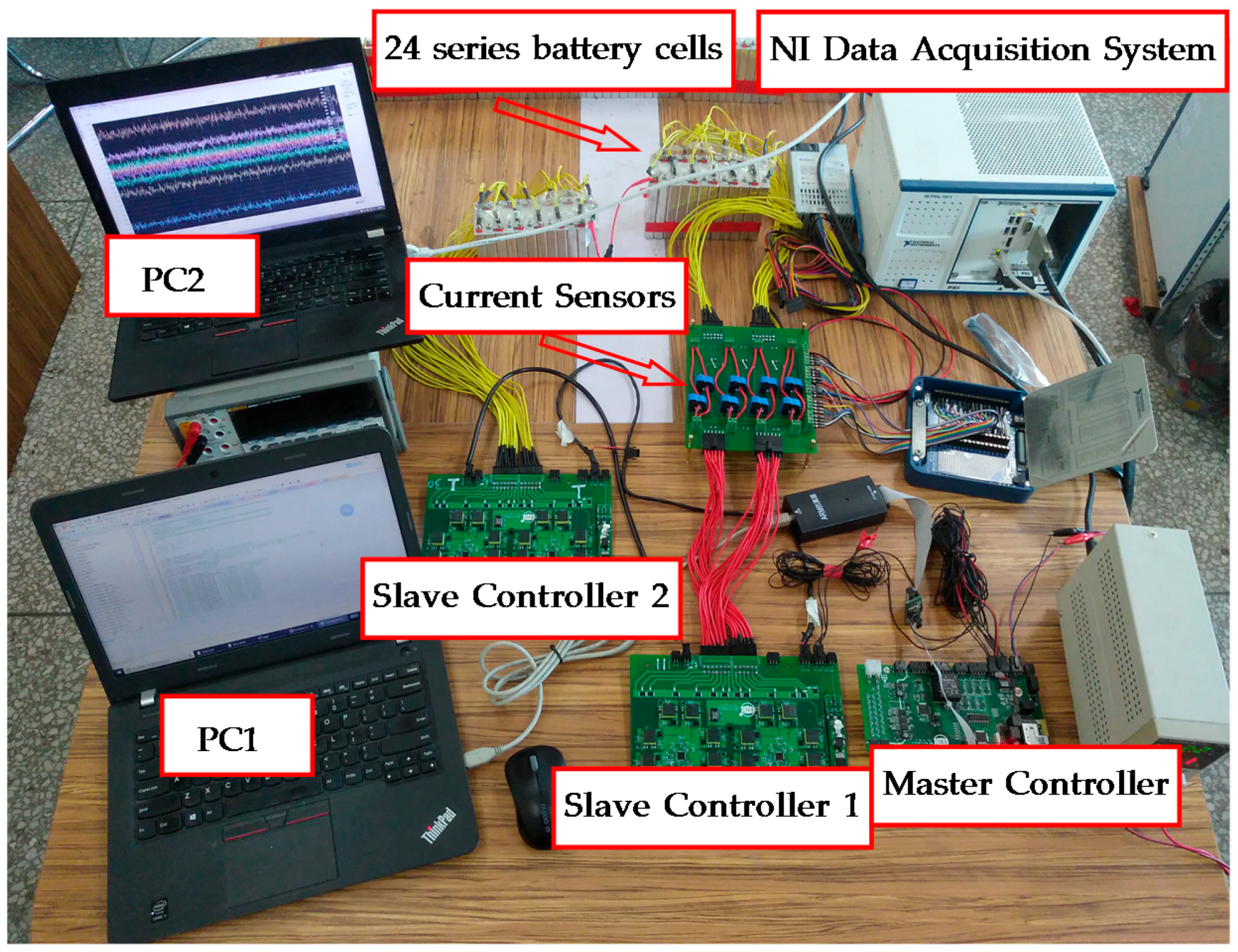
Figure 26 shows that the battery pack contains 24 series cells (lithium titanate), and the capacity of each battery is 2.9 Ah. The maximum balanced capacity of the bidirectional synchronous fly-back balanced circuit is ±4 A. The cell and neighbouring module can be treated as a C2S topology. The fast MPC algorithm, based on the SOC of each battery, determines the balance current needed for each cell. Then, adjusting the balance current is achieved by controlling the time of equilibrium circuit that is working in a balanced cycle, and the battery cell is balanced according to the local optimal equilibrium current.
The specific implementation is to use the MPC algorithm and LP solution function, which is written by the S function and translated into C code using the MATLAB automatic code generation tool. Finally, the C code was downloaded to the BMS main control circuit board through the Keil compiler.
Figure 26 illustrates the experimental bench.
The battery pack consists of two 12 series modules. Twenty-four strings of cells and two slave controllers are used, and a 14-channel Hall-type current sensor is utilised to measure the magnitude of the equalisation current in controller 1. PC1 is used to debug the master controller, which controls the equalisation function of controllers 1 and 2, whereas PC2 is used to record the collected current value.
The voltage values of the first six cell cells are set according to Table 1, and the voltage difference of the cells is approximately 0.5 V. Figure 25 demonstrates the balanced current collected by the NI data acquisition system. This figure shows that, based on the common equalisation control rules, the five other channel currents frequently change direction during equalisation except for the equalisation current direction of cell 1. By contrast, the equalisation currents for all cells do not change direction based on the equalisation process of the MPC rules. The current in the equilibrium period in a graph (a) is either a positive or negative maximum; whereas in graph (b), the equilibrium current of each circuit in a control period is controlled by the duty cycle in a control period. The duty ratio is adjusted to 1 when the maximum balance ability is required. Figure 27b shows the equilibrium current of cell 6. In Table 2, by comparison, under the same initial conditions, the equilibrium time in graph (a) is 1030 s, whereas that in graph (b) is 710 s. The equilibrium time is reduced by 31%.
If we use common control rules to balance the current between cells in the battery pack without decoupling the equilibrium process, then the direction of the balanced current will change frequently. This case makes the battery cells charge and discharge repeatedly, damages the life of the battery and increases the balance time. Hence, this type of control is not advisable despite its simplicity. Using equalisation based on the MPC rules, the overall analysis of the battery cell’s equalisation is performed. The mutual influence between the balanced cells is considered and the decoupling of the equilibrium process is achieved. Therefore, the equalisation current, which is calculated by the optimal algorithm, is used. Repeated changes do not appear in the balance current direction. In addition, the equalisation current is controlled by the duty cycle, and an adjustable equalisation current is output on the fixed balance capability of the hardware, which is an important innovation of this study.
6. Summary
This study introduces the method of using MPC algorithm on distributed DC–DC equalisation circuit and compares the effect of using the algorithm. The optimisation results show that the MPC algorithm can avoid unnecessary energy transfer and shorten equalisation time. The MPC equilibrium scheme is compared with the common equilibrium mode through bench experiments. The experimental result indicates that the equilibrium time is reduced by 31%, which verifies the rationality of the use of MPC algorithm. The algorithm presented in this study can be applied to the active equalisation of a series of battery packs and realise energy transfer with minimum time and high efficiency to make the battery reach equilibrium. This paper improve the active equivalent efficiency through MPC, which can be used as new engineering technology. The key of this method is that the balance current is adjustable. However, the computation process of local optimal solutions is a time consuming process; In the future, other optimization algorithm should be tried to reduce the computation time, which will shorten equilibrium period and increase efficiency further.
Author Contributions
S.S.: testing and writing manuscript; F.X.: designing the control strategies and writing manuscript; S.P.: developing the control system and data analysis; C.S.: organizing the research work and designing the control strategies; Y.S.: developing the control system, designing and building the test bench.
Funding
This research is funded by the Key Tackling Item in Science and Technology Department of Jilin Province, China Grant number [20150204017GX], Jilin Provincial Natural Science Foundation, China Grant number [20150101037JC].
Conflicts of Interest
The authors declare no conflict of interest.
References
- Repp, S.; Harputlu, E.; Gurgen, S.; Castellano, M.; Kremer, N.; Pompe, N.; Woerner, J.; Hoffmann, A.; Thomann, R.; Emen, F.M.; et al. Synergetic effects of Fe3+ doped spinel Li4Ti5O12 nanoparticles on reduced graphene oxide for high surface electrode hybrid supercapacitors. Nanoscale 2018, 10, 1877–1884. [Google Scholar] [CrossRef] [PubMed]
- Wang, X.; Cheng, K.W.E.; Fong, Y.C. Non-Equal Voltage Cell Balancing for Battery and Super-Capacitor Source Package Management System Using Tapped Inductor Techniques. Energies 2018, 11, 1037. [Google Scholar] [CrossRef]
- Genc, R.; Alas, M.O.; Harputlu, E.; Repp, S.; Kremer, N.; Castellano, M.; Colak, S.G.; Ocakoglu, K.; Erdem, E. High-Capacitance Hybrid Supercapacitor Based on Multi-Colored Fluorescent Carbon-Dots. Sci. Rep. 2017, 7, 11222. [Google Scholar] [CrossRef] [PubMed]
- Hoque, M.M.; Hannan, M.A.; Mohamed, A.; Ayob, A. Battery charge equalization controller in electric vehicle applications: A review. Renew. Sustain. Energ. Rev. 2017, 75, 1363–1385. [Google Scholar] [CrossRef]
- Omar, N.; Daowd, M.; Hegazy, O.; Mulder, G.; Timmermans, J.M.; Coosemans, T.; Van den Bossche, P.; Van Mierlo, J. Standardization Work for BEV and HEV Applications: Critical Appraisal of Recent Traction Battery Documents. Energies 2012, 5, 138–156. [Google Scholar] [CrossRef] [Green Version]
- Diao, W.P.; Xue, N.; Bhattacharjee, V.; Jiang, J.C.; Karabasoglu, O.; Pecht, M. Active battery cell equalization based on residual available energy maximization. Appl. Energy 2018, 210, 690–698. [Google Scholar] [CrossRef]
- Wang, Y.J.; Zhang, C.B.; Chen, Z.H. An adaptive remaining energy prediction approach for lithium-ion batteries in electric vehicles. J. Power Sources 2016, 305, 80–88. [Google Scholar] [CrossRef]
- Wang, S.L.; Shang, L.P.; Li, Z.F.; Deng, H.; Li, J.C. Online dynamic equalization adjustment of high-power lithium-ion battery packs based on the state of balance estimation. Appl. Energy 2016, 166, 44–58. [Google Scholar] [CrossRef]
- Moo, C.S.; Hsieh, Y.C.; Tsai, I.S.; Cheng, J.C. Dynamic charge equalisation for series-connected batteries. IEE P-Elect. Power Appl. 2003, 150, 501–505. [Google Scholar] [CrossRef]
- Kutkut, N.H.; Wiegman, H.L.N.; Divan, D.M.; Novotny, D.W. Design considerations for charge equalization of an electric vehicle battery system. IEEE Trans. Ind. Appl. 1999, 35, 28–35. [Google Scholar] [CrossRef] [Green Version]
- Wu, Z.; Ling, R.; Tang, R.L. Dynamic battery equalization with energy and time efficiency for electric vehicles. Energy 2017, 141, 937–948. [Google Scholar] [CrossRef]
- Fong, Y.C.C.; Cheng, K.W.E.; Raman, S.R.; Wang, X. Multi-Port Zero-Current Switching Switched-Capacitor Converters for Battery Management Applications. Energies 2018, 11, 1934. [Google Scholar] [CrossRef]
- Moo, C.S.; Hsieh, Y.C.; Tsai, I.S. Charge equalization for series-connected batteries. IEEE Trans. Aerospace Electron. Syst. 2003, 39, 704–710. [Google Scholar] [CrossRef]
- Ma, Y.; Duan, P.; Sun, Y.S.; Chen, H. Equalization of Lithium-Ion Battery Pack Based on Fuzzy Logic Control in Electric Vehicle. IEEE Trans. Ind. Electron. 2018, 65, 6762–6771. [Google Scholar] [CrossRef]
- Fan, F.L.; Tai, N.L.; Zheng, X.D.; Huang, W.T.; Shi, J.X. Equalization Strategy for Multi-Battery Energy Storage Systems Using Maximum Consistency Tracking Algorithm of the Conditional Depreciation. IEEE Trans. Energy Convers. 2018, 33, 1242–1254. [Google Scholar] [CrossRef]
- Chen, Y.; Liu, X.F.; Fathy, H.K.; Zou, J.M.; Yang, S.Y. A graph-theoretic framework for analyzing the speeds and efficiencies of battery pack equalization circuits. Int. J. Electron. Power Energy Syst. 2018, 98, 85–99. [Google Scholar] [CrossRef]
- Liu, X.T.; Wan, Z.H.; He, Y.; Zheng, X.X.; Zeng, G.J.; Zhang, J.F. A Unified Control Strategy for Inductor-Based Active Battery Equalisation Schemes. Energies 2018, 11, 405. [Google Scholar] [CrossRef]
- Kobzev, G.A. Switched-capacitor systems for battery equalization. In Proceedings of the 6th International Scientific and Practical Conference of Students, Post-graduates and Young Scientists. Modern Techniques and Technology. MTT’2000 (Cat. No.00EX369), Tomsk, Russia, 3 March 2000; pp. 57–59. [Google Scholar]
- Baronti, F.; Roncella, R.; Saletti, R. Performance comparison of active balancing techniques for lithium-ion batteries. J. Power Sources 2014, 267, 603–609. [Google Scholar] [CrossRef]
- Kim, M.Y.; Kim, J.W.; Kim, C.H.; Cho, S.Y.; Moon, G.W. Automatic Charge Equalization Circuit Based on Regulated Voltage Source for Series Connected Lithium-Ion Batteries. In Proceedings of the IEEE International Conference on Power Electronics and Ecce Asia, Jeju, Korea, 30 May–3 June 2011; pp. 2248–2255. [Google Scholar]
- Kutkut, N.H. A Modular Nondissipative Current Diverter for EV Battery Charge Equalization. In Proceedings of the APEC 1998 Thirteenth Annual Applied Power Electronics Conference and Exposition, Anaheim, CA, USA, 15–19 February 1998; Volume 2, pp. 686–690. [Google Scholar]
- Kutkut, N.H.; Divan, D.M. Dynamic equalization techniques for series battery stacks. In Proceedings of the 1996 International Telecommunications Energy Conference, Boston, MA, USA, 6–10 October 1996; 1996; pp. 514–521. [Google Scholar]
- Zhang, Z.L.; Gui, H.D.; Gu, D.J.; Yang, Y.; Ren, X.Y. A Hierarchical Active Balancing Architecture for Lithium-Ion Batteries. IEEE Trans. Power Electron. 2017, 32, 2757–2768. [Google Scholar] [CrossRef]
- Narayanaswamy, S.; Kauer, M.; Steinhorst, S.; Lukasiewycz, M.; Chakraborty, S. Modular Active Charge Balancing for Scalable Battery Packs. IEEE Trans. Large Scale Integr. Syst. 2017, 25, 974–987. [Google Scholar] [CrossRef]
- Wang, Y.J.; Zhang, C.B.; Chen, Z.H.; Xie, J.; Zhang, X. A novel active equalization method for lithium-ion batteries in electric vehicles. Appl Energy 2015, 145, 36–42. [Google Scholar] [CrossRef]
- Shang, Y.L.; Zhang, C.H.; Cui, N.X.; Guerrero, J.M. A Cell-to-Cell Battery Equalizer With Zero-Current Switching and Zero-Voltage Gap Based on Quasi-Resonant LC Converter and Boost Converter. IEEE Trans. Power Electron. 2015, 30, 3731–3747. [Google Scholar] [CrossRef] [Green Version]
- McCurlie, L.; Preindl, M.; Emadi, A. Fast Model Predictive Control for Redistributive Lithium-Ion Battery Balancing. IEEE Trans. Ind. Electron 2017, 64, 1350–1357. [Google Scholar] [CrossRef]
- Caspar, M.; Hohmann, S. Optimal Cell Balancing with Model-based Cascade Control by Duty Cycle Adaption. IFAC Proc. Vol. 2014, 47, 10311–10318. [Google Scholar] [CrossRef]
- Preindl, M.; Danielson, C.; Borrelli, F. Performance Evaluation of Battery Balancing Hardware. In Proceedings of the 2013 European Control Conference (ECC), Zurich, Switzerland, 17–19 July 2013; pp. 4065–4070. [Google Scholar]
Figure 1.
Principle of flying capacitor balance.

Figure 2.
Principle of switch capacitor balance. (a) Energy transfer from cell to capacitor; (b) Energy transfer from capacitor to cell.
Figure 2.
Principle of switch capacitor balance. (a) Energy transfer from cell to capacitor; (b) Energy transfer from capacitor to cell.

Figure 3.
Balance principle of inductors in adjacent cells.

Figure 4.
Balance principle of one inductor in a battery stack.

Figure 5.
Principle of multi-winding transformer balance.

Figure 6.
Principle of multi-transformer balance.

Figure 7.
Principle of switching transformer balance.

Figure 8.
Principle of distributed DC–DC active balance.

Figure 9.
Principle of centralised DC–DC active balance.

Figure 10.
Bidirectional equilibrium schematic.

Figure 11.
Block diagram of main control unit.

Figure 12.
Slave controller.

Figure 13.
Master controller.

Figure 14.
Experimental communication control process.

Figure 15.
Slave controllers and battery pack.

Figure 16.
Voltage equalisation curves of the first battery module.

Figure 17.
Equilibrium at initial stage.

Figure 18.
Equilibrium at final stage.

Figure 19.
Schematic of model predictive control.

Figure 20.
Distributed DC–DC equalisation model.

Figure 21.
DC–DC simulation model.

Figure 22.
Based on the general control.

Figure 23.
Based on the MPC.

Figure 24.
14-channel Hall-type current sensors.

Figure 25.
NI data acquisition system.

Figure 26.
Active balance test bench.

Figure 27.
Comparison of actual current measurement. (a) Based on the general control method; (b) Based on the MPC method.
Figure 27.
Comparison of actual current measurement. (a) Based on the general control method; (b) Based on the MPC method.


Table 1.
Initial state of cells.
| Index | Cell 1 | Cell 2 | Cell 3 | Cell 4 | Cell 5 | Cell 6 |
|---|---|---|---|---|---|---|
| SOC | 0.956 | 0.869 | 0.725 | 0.678 | 0.627 | 0.428 |
| Voltage (V) | 2.687 | 2.634 | 2.528 | 2.501 | 2.255 | 2.164 |
Equilibrium aims to maintain the SOC difference among all cells at less than 3%.
Table 2.
Equilibrium time comparison.
| Method | General Control | MPC | Time Reduced |
|---|---|---|---|
| Time (s) | 1030 | 710 | 31% |
© 2018 by the authors. Licensee MDPI, Basel, Switzerland. This article is an open access article distributed under the terms and conditions of the Creative Commons Attribution (CC BY) license (http://creativecommons.org/licenses/by/4.0/).
Share and Cite
MDPI and ACS Style
Song, S.; Xiao, F.; Peng, S.; Song, C.; Shao, Y. A High-Efficiency Bidirectional Active Balance for Electric Vehicle Battery Packs Based on Model Predictive Control. Energies 2018, 11, 3220. https://doi.org/10.3390/en11113220
AMA Style
Song S, Xiao F, Peng S, Song C, Shao Y. A High-Efficiency Bidirectional Active Balance for Electric Vehicle Battery Packs Based on Model Predictive Control. Energies. 2018; 11(11):3220. https://doi.org/10.3390/en11113220
Chicago/Turabian StyleSong, Shixin, Feng Xiao, Silun Peng, Chuanxue Song, and Yulong Shao. 2018. "A High-Efficiency Bidirectional Active Balance for Electric Vehicle Battery Packs Based on Model Predictive Control" Energies 11, no. 11: 3220. https://doi.org/10.3390/en11113220
Note that from the first issue of 2016, this journal uses article numbers instead of page numbers. See further details here.