Life Cycle Cost of Heat Supply to Areas with Detached Houses—A Comparison of District Heating and Heat Pumps from an Energy System Perspective

Abstract

There are different views on whether district heating (DH) or heat pumps (HPs) is or are the best heating solution in order to reach a 100% renewable energy system. This article investigates the economic perspective, by calculating and comparing the energy system life cycle cost (LCC) for the two solutions in areas with detached houses. The LCC is calculated using Monte Carlo simulation, where all input data is varied according to predefined probability distributions. In addition to the parameter variations, 16 different scenarios are evaluated regarding the main fuel for the DH, the percentage of combined heat and power (CHP), the DH temperature level, and the type of electrical backup power. Although HP is the case with the lowest LCC for most of the scenarios, there are alternatives for each scenario in which either HP or DH has the lowest LCC. In alternative scenarios with additional electricity transmission costs, and a marginal cost perspective regarding the CHP investment, DH has the lowest LCC overall, taking into account all scenarios. The study concludes that the decision based on energy system economy on whether DH should expand into areas with detached houses must take local conditions into consideration.

1. Introduction

One way to achieve energy efficiency in the building sector, and to help avoid global warming and climate change caused by human beings, is to set requirements for buildings’ energy demand. Another way is to focus on and make the supply side of the energy system more efficient and renewable. Both these approaches are mentioned by Lund et al. [1]. The demand and supply side are, however, not two separate distinct systems. There are connections between them, as there are also connections between different supply systems. In Sweden, the majority of the energy supply to buildings consists of district heating (DH) and electricity [2]. In this case, there are connections between the DH system and the electricity system, both through the supply side due to the use of combined heat and power (CHP) where both DH and electricity are produced, and through the demand side due to both DH and electricity being used for heating. A change of heating system in the demand side from DH to a heat pump (HP) will affect both the DH system and the electricity system. It is not likely that climate and environmental goals can be achieved through actions on one side only. Both the demand and supply side need to be improved, not separately, but through joint ventures, to avoid sub-optimization of the systems. DH is a system which is dependent on connection to a large proportion of the heat market to make the distribution more efficient with lower heat losses. Assuming that DH is an effective solution for the buildings, it would then be ineffective from an energy system perspective to have DH in areas together with other heating systems, such as, for example, HPs. Therefore, the demand side and the supply side need to cooperate in order to produce a total system that is as efficient as possible.

DH has been shown to contribute with valuable services which are helpful in an energy system with a high share of variable renewable sources [3,4,5,6,7,8]. Lund et al. point out the importance of looking at the total energy system and not electricity and DH systems as separate parts, and illustrate, for example, the significance of using CHP plants to ensure voltage and frequency stability in the electricity supply [7]. A higher share of DH based on CHP not only increases the electricity production, but also reduces the electricity used for heating. Both these aspects contribute to securing enough electrical power during winter peaks [9]. An expansion of DH in Europe has been shown to reduce greenhouse gas emissions by the same amount as the alternative electrification scenarios proposed by the European Union, but at a lower cost [10]. DH has also been shown to help reach lower greenhouse gas emissions when compared to HPs, assuming fossil marginal electricity production, in Swedish case studies [11,12].

HPs have also been shown to contribute to the integration of variable renewable energy sources, such as wind power. An example is given by Hedegaard et al. [13], where HPs instead of oil boilers and electric heating have been shown to contribute to wind power integration and to reducing fuel consumption in the system. Furthermore, Persson et al. [14] have shown that the change to HPs results in a reduced system cost and reduced carbon dioxide emissions, where the main benefit is a reduced demand for backup power.

Lund et al. concluded that the best way to reach a 100% renewable energy system in Denmark is to combine an expansion of DH in the direct vicinity of existing DH networks, in combination with HPs in other areas [1]. Persson et al. have also shown that there is a potential to increase the share of DH in Europe in total [15]. Sweden is a country with a well-established DH system. However, only roughly 50% of the heat market in Sweden is covered by DH, with the other half covered mostly by electricity-based heating systems, such as HPs [16]. There is a potential to increase the share of DH in Sweden, primarily in the areas with detached houses [17]. So, the question is, should Swedish DH expand into areas with detached houses or should these houses install HPs? There are different views on how effective an expansion of DH is for the environment, compared to HPs. This is mainly due to different assumptions regarding the future production mix, and in particular, the future electricity production mix. This article does not intend to examine this in further detail. Instead, this article aims to answer the economic part of this question by analyzing the energy system cost for an expansion of DH to areas with detached houses, compared to HPs. For DH, this means, for example, that the electricity production from CHP units is credited by the cost for the corresponding electricity production units needed for the same production.

The economic profitability of DH in areas with low heat densities has previously been studied by Reidhav and Werner [18]. However, the study did not include the whole energy system, but focused instead on the profitability for the DH companies. Several other techno-economic, socio-economic, and consumer-economy analyses have been conducted regarding DH in general [10,19,20,21,22]. Grundahl et al. conclude that when a consumer-economy is considered, DH can be shown to be less feasible than if a socio-economy is considered. This emphasizes the importance of a broader system approach. A few of the techno and socio-economic studies mentioned include the surrounding energy system, such as the electricity system, when calculating the economics of DH. However, a more comprehensive analysis where uncertain parameters, such as future costs, are considered is missing. Therefore, apart from considering a wider system perspective where both the DH production system and the electricity production system are included, uncertain parameters such as DH connection share, different types of production units, and their corresponding costs are taken into account using Monte Carlo simulation, where the parameters are randomly sampled from a defined probability distribution for each parameter.

2. Methods

DH and HPs for detached houses are compared to one another using a socio-economic perspective, where the costs for the surrounding energy system, in this case the DH production system and the electricity production system, are considered. The cost is calculated using a life cycle cost (LCC) analysis. LCC analyses calculate the total cost over the lifetime of the product or system analyzed. In this analysis, several units with different lifetimes are included. A project lifetime is therefore set to 25 years, over which the costs are calculated. The costs included are the initial capital cost, annual operation and maintenance (O&M) costs, reinvestment based on the technical lifetime of the equipment in relation to the project lifetime, and residual value due to a longer technical lifetime than the project lifetime, as shown in Equation (1). Residual value considers the remaining value for each equipment based on a linear depreciation.

LCC = ICC + A + R − Res,

(1)

where ICC is the initial capital cost, A is the annual O&M cost, R is the reinvestment cost, and Res is the residual value.

The LCC is calculated using the net present value (NPV) method, where the annual costs, reinvestment cost, and residual value are converted to today’s values using an assumed interest rate. All kinds of taxes and subsidies are excluded.

The comparison is done by calculating the LCC difference between the DH case and the HP case, as shown in Equation (2). A positive LCC_diff means that the DH case is more expensive. The LCC costs for the two cases, DH and HP, are calculated as the mean cost per one building.

LCC_diff = LCC_DH − LCC_HP,

(2)

Due to a lot of uncertain parameters, Monte Carlo simulation is used. In a Monte Carlo simulation, the calculation is done for a defined number of samples, and for each sample, the input parameters are chosen randomly from pre-defined distribution functions. The sample size is set to 100,000. All input data in this analysis is given as truncated normal distributions, with a mean value and a standard deviation. The minimum and maximum values are set to three times the standard deviation, except for physical or mathematical restrictions, such as negative distribution losses.

Parameters that are varied on the building side are the annual heat demand, the heat demand profile, the heat density in the area, and the DH connection share.

The energy system considered is the production, distribution, and installation in the buildings up to and including the DH substation/HP. For the DH case, the distribution costs considered are the cost for the substation and the pipe cost for the distribution system. The production costs considered are the investment costs for the production units and the yearly O&M costs. The production units are dimensioned to cover the buildings’ heat power demand and the distribution losses. The base production is assumed to be CHP, with heat only boilers (HOB) as peak production units. The additional electricity production due to the use of CHP is credited by the corresponding electricity production LCC in the HP case. In the HP case, the heat source is assumed to be geothermal. The costs included are the cost for the HP and the borehole. A COP-value is used to calculate the electricity demand of the building. The electricity production is assumed to be wind power in order to cover the annual energy demand, together with two types of backup power to cover the power demand: gas turbines and hydro power.

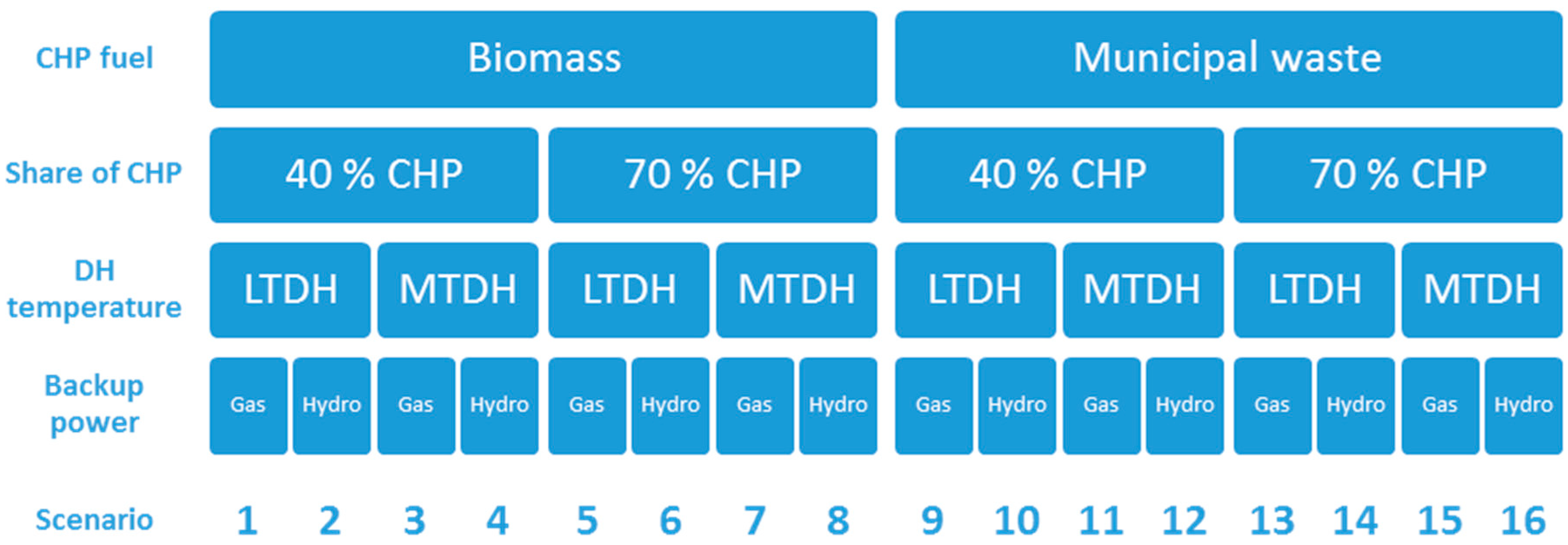
The calculation is done as a base case for 16 different scenarios according to Figure 1, depending on the assumed fuel for the CHP (biomass or municipal waste), the share of CHP, the type of DH distribution (low temperature DH—LTDH, or medium temperature DH—MTDH), and the type of backup power for the electricity production (hydro or gas turbines). For the low temperature DH scenario, the production mix is also changed to include a base load covered by excess heat, which is more accessible with a lower temperature system. In addition, two analyses are done with alternative scenarios in which additional costs for the HP case are included and a marginal cost is assumed for the CHP unit instead of average costs. The alternative scenarios are explained more fully in Section 2.3.

The statistics and prices used are mostly based on national reports from Sweden and Denmark. Local statistics based on the energy system in Falun, Sweden are included as well. Falun is located in the middle of Sweden, in a cold-temperate climate, with an annual average temperature of 4 °C, annual average precipitation of 600 mm, and annual average sun hours of 1600 h [23]. The input data used is found in Section 2.1, with a description of all parameters and their assumptions in the subsections.

2.1. Input Data

All input parameters are found in

Table 1. Input parameters used and their mean value and standard deviation.

Parameter	Unit	Mean Value	Standard Deviation	Reference
Economical parameters
Interest rate	%	3	2
Demand
Heat demand per building	kWh	19,500	5500	Falun * [24]
Heat power demand per annual heat demand	kW/kWh	0.0007	0.0003	Falun *
DH distribution
Heat transmission coefficient	W/m2K	1.55	0.65	[25]
Average pipe diameter	m	0.04	0.01	[25]
Connection share	%	72.5	22.5	Falun *
Cost distribution pipe	EUR/m	370	90	[26]
Distribution pipe length per building	m	25	5	Falun *
Cost service pipe	EUR/m	252	38 **	[26]
Service pipe length	m	15	5	Falun *
Substation cost	EUR	2100	315 **	[27]
Lifetime	Year	40	6 **	[26]
O&M	EUR/kWh	0.0015	0.0005	[26]
Heat pump
Investment cost	EUR	15,000	2250 **	[27]
O&M	EUR/year	278	42 **	[27]
Lifetime	Year	20	3 **	[27]
COP		4.1	0.3	[27]
Biomass CHP
Alpha-value	Electricity/heat	0.35	0.16	[28,29]
Specific investment cost	EUR/kWel,netto	5400	2300	[28,29]
Lifetime	Year	27.5	7.5	[28,29]
O&M fixed	EUR/kWel,netto	189.5	141.5	[28,29]
O&M variable	EUR/kWhel,netto	0.0061	0.0028	[28,29]
Fuel cost	EUR/kWh	0.016	0.001	[2]
Municipal waste CHP
Alpha-value	Electricity/heat	0.255	0.035	[28,29]
Specific investment cost	EUR/kWel,netto	10,000	2300	[28,29]
Lifetime	Year	27.5	7.5	[28,29]
O&M fixed	EUR/kWel,netto	365.65	81.05	[28,29]
O&M variable	EUR/kWhel,netto	0.02535	0.00405	[28,29]
Fuel cost	EUR/kWh	−0.0125	0.002 **	[29]
Biomass HOB
Specific investment cost	EUR/kW	735	165	[28,29]
Lifetime	Year	27.5	7.5	[28]
O&M fixed	EUR/kW	22.75	16.25	[28,29]
O&M variable	EUR/kWh	0.0007	0.0003	[28,29]
Fuel cost	EUR/kWh	0.025	0.004 **	[2]
Wind power
Annual electricity production per installed power	kWh/kW	2850	250	[28]
Specific investment cost	EUR/kW	1260	341	[30]
O&M fixed	EUR/kW	50	14	[30]
O&M variable	EUR/kWh	0.026	0.017	[30]
Lifetime	Year	27	4 **	[27]
Backup power gas
Need of gas	%	40	5	***
Investment cost	EUR/kW	650	350	[28,29]
Lifetime	Year	25	4 **	[28,29]
O&M fixed	EUR/kW	19.5	3 **	[28]
O&M variable	EUR/kWh	0.006	0.001	[28]
Fuel cost	EUR/kWh	0.06	0.01 **	[31]
Efficiency	%	0.35	0.05	[28,29]
Backup power hydro
Need of hydro	%	30	5	***
Investment cost	EUR/kW	265	168	[32]
Lifetime	Year	50	8 **	[32]
O&M total	EUR/kWh	0.02	0.003 **	[32]
Annual share produced in backup power plant	%	30	5	***
Low temperature scenario
Cost excess heat	EUR/kWh	0.01	0.005
Cost distribution pipe	EUR/m	295	20	[26]
Cost service pipe	EUR/m	252	38 **	[26]

* Based on experience and/or statistics in the municipality of Falun, Sweden; ** 15% of the mean value; *** See Section 2.1.6.

. An exchange rate of 10.5 for EUR to SEK has been used for costs in Swedish kronor (SEK) found in some references. An explanation of the parameters and the assumptions made is found in Section 2.1.1, Section 2.1.2, Section 2.1.3, Section 2.1.4, Section 2.1.5 and Section 2.1.6. Where the references have not mentioned an uncertainty span, a standard deviation of 15% of the mean value is assumed.

2.1.1. Economical Parameters

The interest rate used to discount future costs to today’s value is the real interest rate, and is assumed to be 3%. This value of 3% is also the interest rate used in other socio-economic analyses on DH [33,34]. Higher social interest rates are, however, sometimes used; a 3.5% real interest rate is recommended and used by the Swedish Transport Administration [35] and a 4.5% real interest rate is used by the Swedish Energy Markets Inspectorate [36]. One can also argue that social interest rates should be lower in order to invest in future generations. A standard deviation of 2% is therefore used.

2.1.2. Heat Demand

The annual heat demand for detached houses is based on both national statistics [24] and the average demand for all detached houses in the Swedish municipality of Falun. The heat power demand, i.e., the maximum hourly heat demand, in relation to its annual energy demand (kW/kWh), is based on the average of the detached houses in Falun. The heat power demand and the heat demand profile are, among others, used to dimension the production units.

2.1.3. DH Distribution

The DH is assumed to be medium temperature DH (MTDH), the same temperature levels as most of the DH networks in Sweden, also called 3rd generation DH. The DH distribution costs included are the investment cost for the pipes and the yearly O&M costs. The investment costs for the pipes are calculated using Equation (3) below.

$$C_{distr}=C_{dp}\times \frac{l_{dp}}{SH}+C_s\times l_s+C_{ss}$$

(3)

where C_distr is the total distribution cost [EUR], C_dp is the distribution pipe cost per meter [EUR/m], l_dp is the average distribution pipe length per building [m], SH is the connection share, C_s is the service line cost per meter [EUR/m], l_s is the service line length [m], and C_ss is the substation cost [EUR].

The proportion connected is based on the experience of Falun, and is assumed to be in the range of 50% to 95%. The average distribution and service pipe lengths are according to the experience of Falun, with values of 25 ± 5 m and 15 ± 5 m, respectively. Total pipe lengths of 40 ± 10 m correspond well with a Swedish study on sparsely installed DH [37]. The distribution pipe costs are taken as the average for pipes 0–50 kW and 250–1000 kW from a Danish report [26]. The service pipe is assumed to be 0–20 kW, with costs from the same Danish report. The distribution losses are calculated using Equation (4) below.

$$q_{hl}=1/(1+\frac{\left(Q_s/L\right)}{K\times 2\times \pi \times d_a\times G})$$

(4)

where q_hl is the annual share of distribution losses, Q_s is the annual heat sold to the customers [kWh], L is the distribution and service pipe length [m], K is the heat transmission coefficient [W/m²K], d_a is the average pipe diameter [m], and G is the degree time number for heat distribution [°Kh]. K, d_a, and G are based on Swedish figures by Frederiksen and Werner [25]: K and d_a for sparse connection to DH with twin pipes (0.9–2.2 W/m²K and 0.03–0.05 m respectively), and G for average Swedish DH systems (520,000 °Ch). For the LTDH scenario, the distribution losses are assumed to be one fourth of the losses in the MTDH, according to Lund et al. [38]. Not many LTDH networks have been built, but the Danish report [26] states that LTDH might be slightly cheaper to build than MTDH. The service pipes are assumed to be the same, but the distribution pipes are assumed to be plastic flexible pipes in the LTDH scenario. The cost for the distribution pipes is therefore, in the LTDH scenario, taken as the service pipe costs in [26], but for larger pipes (20–100 kW instead of 0–20 kW, as assumed for the service pipes).

2.1.4. Heat Pump

The HP investment cost, O&M cost, lifetime, and COP value are all taken from a Danish reference [27]. The investment cost for the HP is the combined cost for the HP and the associated borehole. The COP value is assumed to be the average for buildings with radiators and underfloor heating. In the calculation, the COP value is assumed to be constant over the year.

2.1.5. DH Production

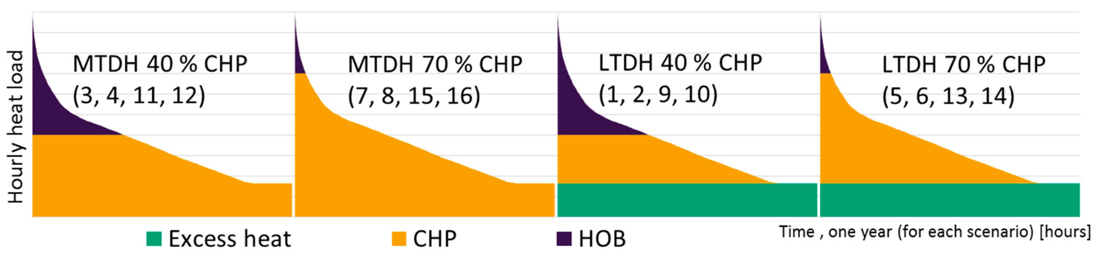
The DH is assumed to be produced using CHP as the base and HOB as the peak. Two different scenarios are used to calculate the cost for two different percentages of CHP. The two different percentages assumed are that CHP covers 40% and 70%, respectively, of the heat power demand. There are also two different scenarios regarding the fuel used in the CHP unit. The two different fuels considered are biomass and municipal waste. The HOB is assumed to be biomass-based for both cases. The biomass assumed for the CHP unit is a mix of wood chips and forest residue, and the biomass assumed for the HOB unit is pellets. Pellets as fuel for the HOB, instead of wood chips, are chosen as wood chips require more advanced equipment and represent a more bulky fuel, which is not suitable for peak boilers. In the scenario with low temperature DH, the DH production is also assumed to change, with a base of excess heat from industries. The excess heat is assumed to cover 15% of the heat power demand. An illustrative picture of the different scenarios regarding the share of CHP and LTDH with excess heat is shown in Figure 2.

The capital costs for the production units are based on their dimensions, which in turn depend on the heat power demand. It is also assumed that the CHP units produce at their maximum during the whole year, which means that the HOB are only in operation at hours where the demand is greater than the installed CHP capacity. The annual energy delivery, and thereby the fuel demand, is based on the hourly demand profile of the detached houses. The cost for the biomass CHP is for a unit between 20–80 MW feed, and the cost for the municipal waste CHP is for a unit handling 35–80 MW feed [28,29].

The electricity production from the CHP units is calculated using the annual average alpha-value [28,29], which describes electricity production per heat production. The alpha-value is assumed to be constant over the year. This electricity production is credited by the cost for the corresponding electricity production in the HP case. This is described in the electricity production section, Section 2.1.6.

2.1.6. Electricity Production

Sweco [39] presents two ways to reach a 100% renewable electricity system in Sweden. In both ways, the nuclear power (roughly 40% of the electricity production in Sweden) is mainly replaced by wind power, dimensioned to produce the same annual electricity. The two ways then differ regarding the backup power that supports the wind power. Either the existing hydro power is upgraded in order to increase the power capacity, or gas turbines are built. Gas turbines can be fueled, for example, with biogas or bio oil, in order to reach a 100% renewable system. Based on this, it is assumed that wind power is dimensioned to cover the annual energy demand for the HP case. The two different backup power alternatives, upgrading hydro power or building gas turbines, are calculated as two different scenarios.

Based on the possible future energy mix in the Swecos report [39], with the difference that the power balance is assumed to be covered nationally and that other smaller backup power units are assumed to be hydro or gas, it is calculated that the backup power demand in the case of upgraded hydro power is 0.25 units of hydro power per unit of wind power. For the case of gas turbines, the calculated value is 0.35 units of gas turbines per unit of wind power. The total need for additional reserves according to another Swedish study [40] is said to be 4300–5300 MW, with 12,000 MW additional wind power. This gives 0.36–0.44 units of backup power per unit of wind power. The amount of backup power needed is assumed to be somewhere in between these two, with values of 0.4 ± 0.05 units of gas turbines per unit of wind power and 0.3 ± 0.05 units of additional hydro power capacity per unit of wind power.

The annual energy demand covered by the backup power plants is based on Swedish wind power statistics and the hourly demand profile of detached buildings in Falun. Average Swedish hourly wind power statistics from the Swedish transmission system operator [41] for the years 2013–2016 is scaled to cover the yearly energy demand of the detached house with a HP. This profile is then compared to the hourly demand profile of the building. The result is that approximately 30% of the buildings’ annual demand is not covered by the wind power, but has to be covered by backup power.

The gas turbine costs are for turbines with a capacity of 5–40 MW. The fuel for gas turbines is assumed to be bio oil, in order to have a renewable solution, with costs from the Swedish Energy Agency [31]. The cost for upgrading the capacity of hydro power is taken from Krönert et al. [32]. The cost for upgrading is assumed to be the average for hydro power turbines between 10–225 MW. This is within the same range as the cost for adding a turbine to an existing dam constructed for other reasons, according to a report by the International Renewable Energy Agency [30].

2.2. Parameter Study

A linear regression is done to study the effect of the different parameters on the result. Correlation coefficients are calculated between the result and each parameter. Correlation coefficients describe the statistical relationship between two variables (in this case, each parameter and the result), and vary between −1 and 1. The value of −1 represents the maximum negative relation, i.e., a higher value for the parameter results in a lower value for the result. The value of +1 represents the maximum positive relation, i.e., a higher value for the parameter results in a higher value for the result. The value of 0 indicates that there is no correlation between the parameter and the result. There can, however, be a relation between the variables, but not a linear one. The five parameters with the highest absolute correlation coefficients are presented for each scenario.

2.3. Alternative Scenarios

Even though a lot of uncertainties are handled in the Monte Carlo simulation, the values of the parameters are for a particular basic assumption for each parameter. For example, the CHP investment cost is assumed to be the average cost. Another assumption could be that the CHP investment cost is based on the marginal cost. Two different basic assumptions are handled in two alternative scenarios. The first, alternative scenario A, assumes an additional cost for investments in the transmission grid, demand response flexibility, and energy storage, and the other assumes, as the example above, a marginal instead of average CHP investment cost.

In the two ways presented to reach a 100% renewable electricity system in Sweden presented by Sweco [39], on which the scenarios in this study are based, additional investments in the transmission grid, demand response flexibility, and energy storage are also included. It is stated that these costs are associated with great uncertainty. These costs are specific to each situation, depending on, for example, the transmission distance and current flexibility in the system. They are therefore not included in the base case, which only includes the production unit costs and the local DH distribution cost. They are instead included in alternative scenario A. The costs in total for additional investments in the electricity grid, demand response flexibility, and energy storage are estimated to be approximately 29 billion euros in the Swedish case. This results in approximately 1600 EUR/kW of additional installed wind power capacity in the scenarios. This cost is added to the HP case in the alternative scenario A, in order to analyze how the LCC_diff value changes. Note again, this cost is associated with great uncertainty and should be treated as “if additional costs of this amount arise, this is what happens with the difference in LCC”.

The CHP investment cost in the base case is the mean investment cost per installed capacity for the whole CHP plant. One can, however, argue that when a decision has already been made to build a CHP plant, the marginal cost for building a larger CHP plant in order to cover additional customers should be the cost used when calculating the profitability of these additional customers. Using a calculated marginal CHP investment cost is therefore done as a second alternative scenario, alternative scenario B. The mean cost in the base case is the mean cost for two different sizes, for both biofuel- and municipal waste-based CHP. The marginal cost is calculated as the additional cost per installed capacity for the bigger unit, compared to the smaller unit. The resulting specific investment cost for biofuel-based and municipal waste-based CHP is 2700 ± 467 EUR/kW and 8111 ± 1344 EUR/kW, respectively. These can be compared to the mean costs found in Table 1, which are 5400 ± 2300 EUR/kW and 10,000 ± 2300 EUR/kW, respectively.

3. Results

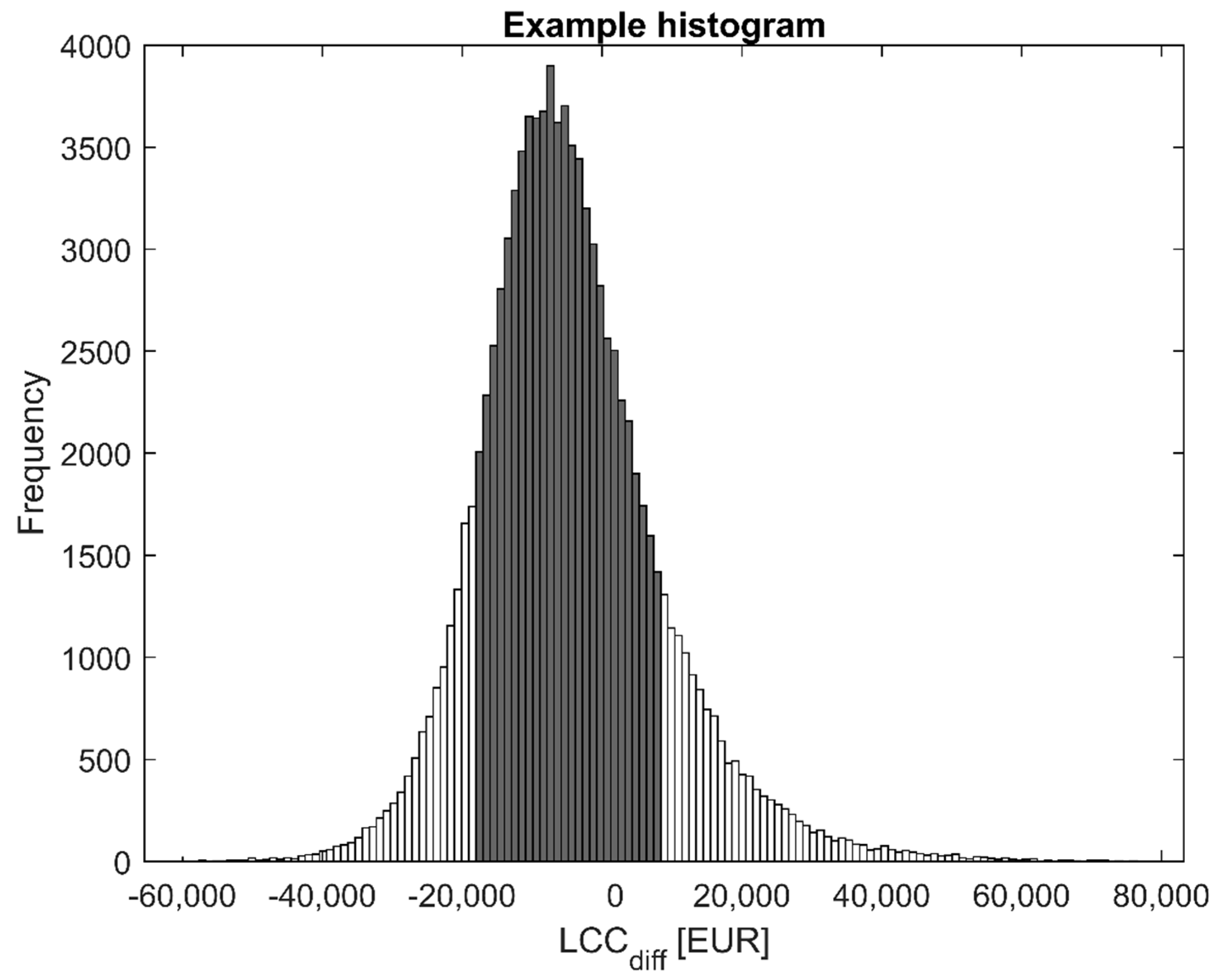
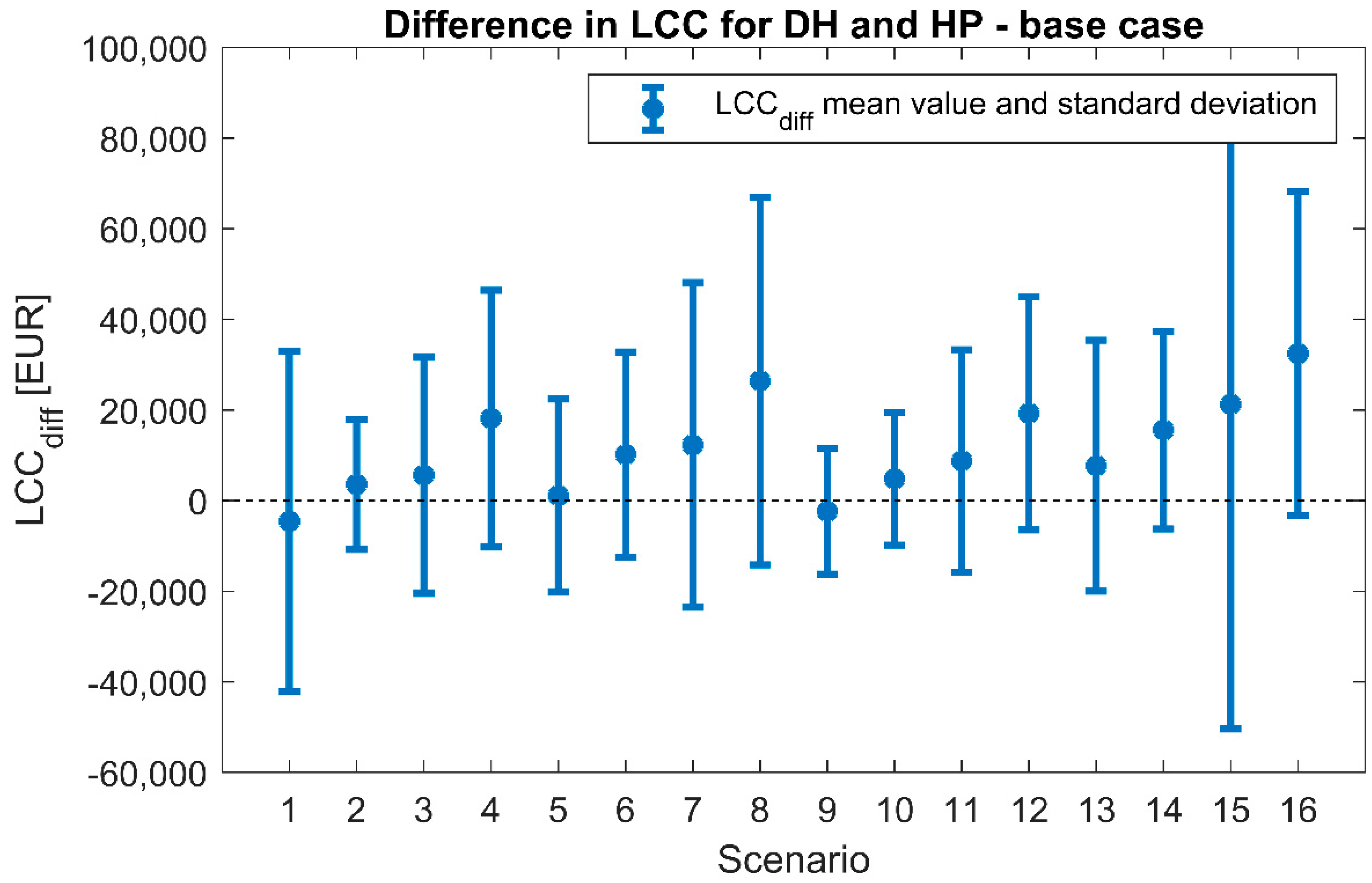
The results for each scenario can be presented as a histogram, see Figure 3 for an example. The resulting LCC_diff is the difference in LCC for the DH case and the HP case. Negative LCC_diff values mean that the DH case has a lower LCC than the HP case. For scenario 1, the mean value is negative, i.e., DH has a lower LCC than the HP case. To make a comparison between the different scenarios, the mean value and the corresponding standard deviation for each scenario are displayed in Figure 4. Compared to the DH case, the HP case ranges from having around a 4000 EUR higher average LCC (scenario 1) to a 32,000 EUR lower average LCC (scenario 16). In relation to the DH LCC, this corresponds to a 16% increased LCC cost and a 53% decreased LCC cost for the HP case, respectively.

Scenarios 1 and 9 are the only two scenarios where the DH case has a lower LCC than the HP case. These are the two scenarios with a low share of CHP, LTDH, and gas as electrical backup power, for CHP units based on biofuel and municipal waste, respectively. The most favorable scenario for DH is biofuel-based LTDH with a small share of CHP and with gas turbines as electrical backup power. Overall, the HP case has a lower LCC. The most favorable scenario for HPs is municipal waste-based MTDH with a high share of CHP and with hydro power as backup power.

3.1. Parameter Study Results

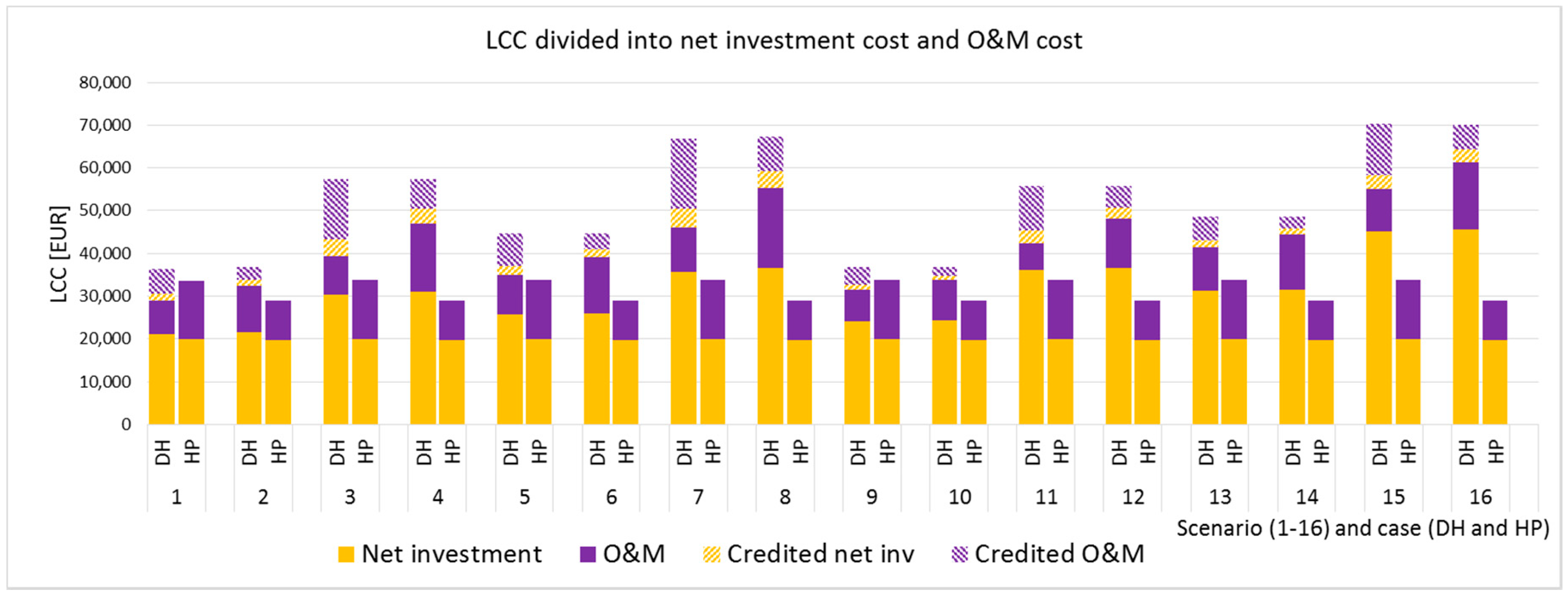
The LCC divided into DH and HP, and the net investment cost and O&M cost, respectively, are found in Figure 5. The net investment cost is calculated as the initial investment cost plus the reinvestment cost, minus the residual value. The credited cost for electricity production using CHP is also included in Figure 5. Without this credited cost, DH would not have the lowest LCC in any of the scenarios. Figure 4 only presents the total LCC_diff, but in Figure 5, the LCC for each case is presented. The lowest LCC for the DH case is the LCC for scenario 1, whereas the lowest LCC for the HP case is for scenario 14. These costs are almost the same. For both cases, DH and HP, the net investment cost is the highest share. The O&M cost represents a higher relative share of the total LCC in the HP case (on average 36% of the total LCC) compared to the DH case (on average 26% of the total LCC).

The five parameters with the highest absolute correlation coefficients for each scenario, i.e., the parameters with the highest correlation with respect to the resulting LCC_diff, are listed in

Table A1. The five parameters with the highest absolute correlation coefficient for each scenario, with the value of the correlation coefficient in brackets.

Scenario	Parameter 1	Parameter 2	Parameter 3	Parameter 4	Parameter 5
1	Distribution losses (0.93)	Distribution maintenance cost (0.89)	Heat power demand (0.20)	Maintenance CHP, fixed (0.09)	Connection proportion (−0.09)
2	Heat power demand (0.55)	Heat demand (0.27)	Distribution maintenance cost (0.26)	Connection proportion (−0.24)	Distribution losses (0.24)
3	Heat power demand (0.55)	Distribution losses (0.44)	Distribution maintenance cost (0.38)	Maintenance CHP, fixed (0.25)	Specific cost CHP (0.21)
4	Heat power demand (0.51)	Distribution maintenance cost (0.36)	Distribution losses (0.36)	Maintenance CHP, fixed (0.23)	Heat demand (0.23)
5	Heat power demand (0.53)	Maintenance CHP, fixed (0.33)	Alpha (0.32)	Specific cost CHP (0.29)	CHP lifetime (−0.18)
6	Heat power demand (0.50)	Alpha (0.38)	Maintenance CHP, fixed (0.32)	Specific cost CHP (0.27)	Heat demand (0.25)
7	Heat power demand (0.52)	Maintenance CHP, fixed (0.31)	Distribution maintenance cost (0.27)	Specific cost CHP (0.27)	Alpha (0.23)
8	Distribution losses (0.47)	Heat power demand (0.47)	Distribution maintenance cost (0.40)	Alpha (0.31)	Maintenance CHP, fixed (0.28)
9	Heat power demand (0.69)	Connection proportion (−0.24)	HP investment cost (−0.19)	CHP lifetime (−0.17)	Wind power O&M variable (−0.16)
10	Heat power demand (0.65)	Distribution maintenance cost (0.31)	Heat demand (0.29)	Distribution losses (0.29)	Connection proportion (−0.24)
11	Heat power demand (0.73)	Distribution losses (0.23)	Distribution maintenance cost (0.21)	Connection proportion (−0.21)	CHP lifetime (−0.18)
12	Heat power demand (0.69)	Distribution maintenance cost (0.33)	Distribution losses (0.28)	Heat demand (0.26)	Connection proportion (−0.20)
13	Distribution losses (0.65)	Distribution maintenance cost (0.62)	Heat power demand (0.55)	CHP lifetime (−0.18)	Heat demand (0.17)
14	Heat power demand (0.70)	Heat demand (0.33)	CHP lifetime (−0.25)	Distribution maintenance cost (0.24)	Specific cost CHP (0.21)
15	Distribution losses (0.88)	Distribution maintenance cost (0.86)	Heat power demand (0.35)	CHP lifetime (−0.11)	Specific cost CHP (0.10)
16	Heat power demand (0.70)	Distribution maintenance cost (0.31)	Heat demand (0.28)	CHP lifetime (−0.22)	Distribution losses (0.20)

in Appendix A. The one parameter that is found in the top five parameters with the highest correlation coefficients in all 16 scenarios is the heat power demand of the buildings as a function of the annual energy demand. This parameter affects the dimension of the production units. The heat power demand as a function of the annual energy demand is found to have a strong or very strong correlation (absolute correlation coefficient above 0.5) in 13 of the scenarios, a moderate correlation (absolute correlation coefficient between 0.3 and 0.5) in two scenarios, and a weak correlation in one scenario. After the heat power demand, the distribution maintenance cost and distribution losses are the two parameters with the highest correlation coefficient in most scenarios. These two parameters refer to the DH distribution cost. The DH distribution losses affect both the dimension of the DH production units and their O&M costs. The distribution maintenance cost has a strong or very strong correlation in three scenarios, a moderate correlation in six scenarios, and a weak correlation in four scenarios. The distribution losses have a strong or very strong correlation in three scenarios, a moderate correlation in three scenarios, and a weak correlation in five scenarios. The heat power demand, the distribution maintenance cost, and the distribution losses are the only parameters with a strong or very strong correlation. Other parameters found in the top five are the building’s heat demand, CHP maintenance cost, CHP lifetime, connection proportion, CHP specific investment cost, alpha-value, and HP investment cost. All of these do, however, have a moderate or weak correlation (absolute correlation coefficient below 0.5).

3.2. Alternative Scenarios

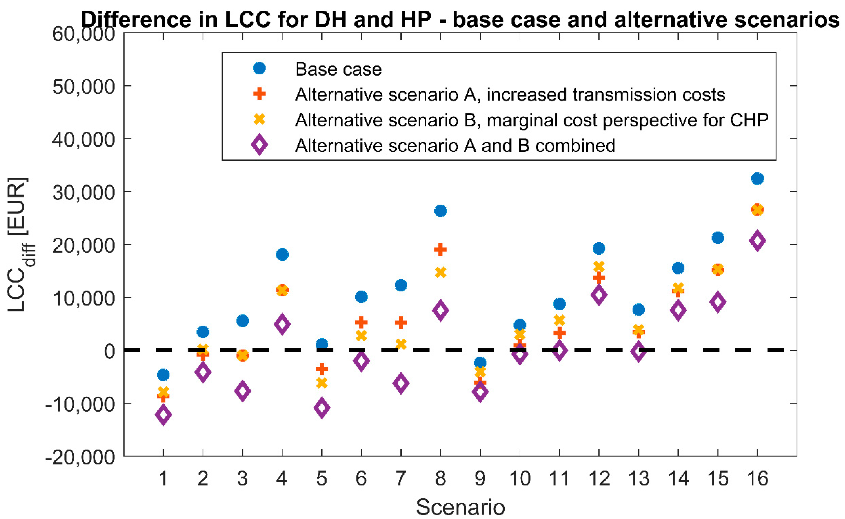
The results for the alternative scenarios are shown in Figure 6, both separately and for the two different alternative scenarios combined. In alternative scenario A, where additional costs are added to the HP case (such as additional costs in the transmission grid, demand response flexibility, and energy storage), DH is the case with the lowest LCC for more scenarios than in the base case. Scenarios 1, 2, 3, 5, and 9 result in a lower LCC for the DH case. The scenario with the lowest LCC for the HP case is scenario 4, with an average LCC of 31,500 EUR. The scenario with the lowest LCC for the DH case is scenario 1, with an average LCC of 27,500 EUR. The overall lowest energy system cost, therefore, changes from HP in the base case, to DH in this alternative scenario. In alternative scenario B, where marginal costs are considered for CHP investment, DH is the case with the lowest LCC for four scenarios: 1, 3, 5, and 9. The scenario with the lowest LCC for the DH case is scenario 1, with a DH average LCC of 26,000 EUR. The scenario with the lowest LCC for the HP case is scenario 16, with an average LCC of 29,000 EUR. Also, in this alternative scenario, the DH case has the overall lowest energy system cost. When the two alternative scenarios are combined, DH is the case with the lowest LCC for ten scenarios. The DH case also has a significantly lower LCC than the HP case: 24,000 EUR in scenario 1, compared to the lowest HP LCC of 31,500 EUR in scenario 14.

4. Discussion

The electricity production in the HP case is assumed to be 100% renewable, with a base of wind power and either hydro power or bio oil fueled gas turbines as backup power. These scenarios are based on possible future scenarios for the Swedish system, but can be generalized to other geographical areas with similar conditions for the different production units. The different DH scenarios are based on the existing DH systems in the Nordic countries, where DH is well-established. Even though a lot of different scenarios have been considered, they might not be relevant everywhere. Wind power is assumed in all scenarios, but one has to consider the scenarios which are relevant to the geographical area, e.g., if hydro power and biomass are available or if it is more suited to gas turbines and municipal waste incineration.

For the base case, counting all scenarios, HP generally has the lowest LCC. In 14 of the 16 scenarios, HP has a lower LCC than DH. However, there are outcomes in all scenarios in which HP or DH is the cheapest alternative. It is therefore important to take local conditions into consideration when analyzing the LCC for HPs vs DH in areas with detached houses. According to the parameter study, the distribution costs have a high correlation, with HP being the case with the lowest LCC. It is necessary to keep these costs down for DH to become the solution with the lowest LCC. The parameter which has the strongest positive correlation with HP being the case with the lowest LCC is the heat power demand as a function of the annual energy demand. Therefore, it is most important is to keep the heat power demand of the buildings low, i.e., a more even demand, in order for DH to become the solution with the lowest LCC. This increases the utilization rate of the CHP production unit, which has a high investment cost and is dependent on a high capacity factor in order to become economically justifiable.

A lower heat production cost (due to the assumption of more excess heat available), and lower distribution costs, are found in the LTDH scenarios. This is why the LTDH scenarios are more favorable for DH. This of course assumes that there is excess heat available in the DH area. Due to the high CHP cost, a lower share of CHP is also more favorable for DH although the electricity production is credited with the value for the corresponding wind power and backup power. Municipal waste-based CHP has a higher investment and O&M cost than biofuel-based CHP, but a much lower fuel price. This lower fuel price does, however, not outweigh the difference in investment and O&M costs. Municipal waste-based CHP also has lower electricity production, meaning that less electricity production is being credited compared to the biofuel-based CHP. There can, however, be other driving forces for municipal waste incineration, when the alternative for the municipal waste is landfill.

Regarding the different backup power scenarios, gas turbines are more expensive than upgraded hydro power plants. This makes gas turbines more favorable for the DH case. The gas turbines in these scenarios are based on bio-oil, which makes the running cost very high. It should also be noted that the low cost for the hydro power scenario is due to an assumption that it is possible to upgrade existing hydro power plants. In the case of newly built hydro power plants, the investment cost is higher, which would give other results. Also, there are natural limitations on if and where hydro power plants can be built.

The difference in the average LCC_diff for the 16 scenarios in the base case, which is around 4000 EUR or 14% lower LCC per building to the DH case advantage (scenario 1), to 32,000 EUR or 53% lower LCC per building to the HP’s advantage (scenario 16), is over the whole calculation period of 25 years. This difference in cost should be set against other benefits for the two cases. An expansion of DH, where DH would replace current electricity-based heating, would, for example, relieve the electricity grid. An expansion of the current electricity grid, i.e., a cost for the system, might not be needed, for example, in order to introduce more electric vehicles to the system. In a more electrified system with a higher share of intermittent power production, there can also be additional costs in order to upgrade the transmission grid or to invest in demand response flexibility or energy storage in order to handle the intermittence. An attempt to analyze how costs such as these would affect the whole energy system cost is done in alternative scenario A. Adding these costs shows that the case with the overall lowest LCC changes from HP to DH, even though HP is still the case with the lowest LCC compared to DH for most of the scenarios studied. The cost for such investments has to be studied further though, as the ones included are associated with great uncertainty.

Another factor that might change the result is economy of scale when bigger plants are built. This will probably affect the DH case more than the HP case, since CHP plants are greatly affected by economy of scale. If DH is already economical for an area with a higher heat density, one can also argue that the marginal increase when investing in a slightly larger production unit, in order to cover the demand in areas with detached houses, should be used when comparing the LCC with an electrified solution using HPs. Using this approach, as in the previous alternative scenario, the case with the overall lowest LCC changes from HP to DH compared to the base case.

When the two different alternative scenarios are combined, the DH case has the lowest LCC in 10 of the 16 scenarios, and the overall average LCC for the scenario with the lowest DH LCC, with a value of 24,000 EUR in scenario 1, is much lower than the overall average LCC for the scenario with the lowest HP LCC, with a value of 31,500 EUR in scenario 14.

Except for the two costs taken into account in the alternative scenarios, there are other aspects that should be taken into consideration, for example, environmental aspects, social aspects, and technical aspects, such as stability in the system. DH, for example, makes it possible to make use of bulky residual resources from industries (for example the forest industry) that would otherwise not be used. Making use of industries’ residues is resource efficient. On the contrary, HPs make it possible to produce heat without any use of fuels, by using wind power and hydro power. An electrified heating system using intermittent power production would, however, result in a more unstable electricity system, compared to a system with a higher share of CHP. Putting a value on these other benefits/impacts may change whether DH or HP has the lowest cost, as the LCC_diff values for the 16 scenarios are quite small and differ between different scenarios and assumptions.

5. Conclusions

The energy system cost for an expansion of DH to areas with detached houses, compared to HPs, is analyzed using Monte Carlo simulation. The cost is calculated over a project lifetime of 25 years, using the net present value method. Parameters varied in the Monte Carlo simulation are, among others, investment and O&M costs, DH connection share, need for backup power, and DH distribution lengths. In addition to these variations of each parameter, 16 different scenarios are evaluated regarding main fuel used, share of CHP, DH temperature level, and type of electrical backup power. Two alternative scenarios are also analyzed regarding the investment costs for the two cases: DH and HP.

The results show that for each scenario, there are combinations of the input parameters that result in either DH or HP being the case with the lowest LCC. In the base case, HP in itself has the lowest LCC overall, considering all scenarios. In the alternative scenarios, where either the cost for the HP case is increased or the cost for the DH case is decreased, the overall lowest LCC is changed to the DH case. There are, however, still combinations of the input parameters that result in either DH or HP being the case with the lowest LCC for each scenario.

Therefore, when deciding if DH should, or should not, expand into areas with detached houses based on economy, it is necessary to take local conditions, both physical and economic, into account. However, it is probably also important to take other aspects into consideration, such as the environmental impact and stability of the systems.