A PLC Channel Model for Home Area Networks

Abstract

Smart meters (SMs) are key components of the smart grid (SG) which gather electricity usage data from residences and businesses. Home area networks (HANs) are used to support two-way communications between SMs and devices within a building such as appliances. This can be implemented using power line communications (PLCs) via home wiring topologies. In this paper, a bottom-up approach is designed and a HAN-PLC channel model is obtained for a split-phase power system which includes branch circuits, an electric panel with circuit breakers and bars, a secondary transformer and the wiring of neighboring residences. A cell division (CD) method is proposed to construct the channel model. Furthermore, arc fault circuit interrupter (AFCI) and ground fault circuit interrupter (GFCI) circuit breaker models are developed. Several HAN-PLC channels are presented and compared with those obtained using existing models.

1. Introduction

Increasing energy demands worldwide have resulted in significant growth in greenhouse gas emissions. As a consequence, government organizations are making efforts to combat climate change and reduce these emissions [1]. One of the approaches is to modernize the power grid infrastructure and use renewable energy sources [2]. These distributed energy resources require effective communications for the management of power transmission and distribution. A power grid with bidirectional communication capabilities to meet these purposes is often referred to as a smart grid (SG) [3,4,5]. Smart meters (SMs) are part of the smart grid which are deployed at residences in place of traditional electric meters.

In North America and Europe, the legislative approval of smart meters has led to an increase in the number of intelligent devices such as smart appliances with a growing market of billions of dollars [6,7]. One of the purposes of SMs is to help both power suppliers and residence owners with power management. Figure 1 shows the average power consumption of residences according to the survey by U.S. Department of Energy in September 2017. The appliances for heating, ventilation and air conditioning (HVAC) and water heating account for approximately half of the power consumed. A smart meter installed in a residence can provide flexibility in managing these appliances to reduce costs.

SMs enable bidirectional communications in a smart grid. They can transmit data to data acquisition centers (DACs) for analysis and receive real time pricing information from the DACs. In a home area network (HAN), SMs collect power usage data from home appliances, send commands to control these appliances, and exchange information with homeowners and tenants. Real time pricing (RTP) allows appliances such as dishwashers, washing machines and dryers to be operated during off-peak times when prices are low [8]. This can also be used to reduce HVAC and water heater costs. Energy theft prevention is another function of SMs. With advanced theft detection and encryption algorithms, SMs can detect and report, as well as prevent illegal electricity usage [9]. Appliance monitoring can also be provided by regularly checking and reporting the status of appliances. Power suppliers can also benefit from SMs as meter data can be obtained remotely which is more cost efficient than manual reading. Power line communications (PLC) can be employed for SM services via a home area network (HAN) [10]. Since the power distribution system was not originally designed for communication purposes, the modeling of power lines as communication channels is critical to the design and analysis of HAN PLC.

Power Line Communications for Home Area Networks

The growing interest in smart home services has prompted research on broadband power line communications (BB-PLC) for high-speed data transmission. IEEE Std 1901-2010 provides networking protocols for broadband communications using power lines [11] while IEEE Std 1901.2-2013 for narrowband power line communications (NB-PLC) assures coexistence with broadband communications [12]. NB-PLC is suitable for the collection of power usage data and so can be used to provide SM services within businesses and residences via HANs. Modulation schemes for PLC communications include binary phase shift keying (BPSK), frequency shift keying (FSK), spread frequency shift keying (S-FSK), spread spectrum (SS), orthogonal frequency division multiplexing (OFDM) or a combination of these techniques [13]. Media access control (MAC) protocols include carrier sense multiple access (CSMA) with collision avoidance (CSMA/CA) and time division multiple access (TDMA). Single-input single-output (SISO), single-input multiple-output (SIMO), multiple-input single-output (MISO) and multiple-input multiple-output (MIMO) techniques have been developed for wireless systems, but are not included in the IEEE BB-PLC and NB-PLC standards.

Previous research on PLC-based smart metering has focused on the links between SMs and DACs [14,15,16,17]. However, there has been little research on PLC for HANs. Thus, further study is required for real home wiring topologies to obtain accurate channel models. Several PLC channel models have been proposed in the literature based on experimental results for specific topologies and so cannot be generalized. In [18], a channel model was developed based on an NEC compliant topology including a panel. However, this model was constructed as a cascaded two-port network with the same path-loss in the phase and neutral conductors, which ignores the fact that they connect to different parts of the panel. In [19,20,21], a HAN-PLC model with a panel was given, but only the bonding strap to ground was considered within the panel. The model in [22] has only five branch circuits which is insufficient to model a HAN network. The panel was modeled as a black box so the results cannot be generalized either. In [23], the influence of normal and ground fault circuit interrupter (GFCI) circuit breakers on PLC was investigated which only from one part of the HAN topology.

An impedance carry back (ICB) method for PLC channel modeling was given in [24]. Figure 2 shows a simple example of this method. The backbone refers to the direct path between the transmitter and receiver, while outlets o₁, o₂ and o₃, and nodes n₁ and n₂ are on an indirect path connected to the backbone at $n_b$. The impedance of the path is calculated following a bottom-up approach from o₁ and o₂ to n₂, and finally to $n_b$ as illustrated in Figure 2 from step (a) to (c). Unfortunately, the use of indirect paths in developing a channel model is difficult for large topologies with a long backbone and many indirect paths. To tackle this problem, a simple and flexible bottom-up approach that can be used for any topology is developed here. In this approach, a generalized cell division (CD) method is applied to the split-phase power system in North American residences.

The contribution of this paper is in the area of power line communications (PLC) in the context of home area networks (HANs). A wiring topology is modeled for North American residences with a split-phase power supply. A smart meter is considered as the PLC transmitter or receiver which is seldom discussed in existing channel models. The parameters of the topology components are obtained and their impedances are derived. A detailed description of the panel is given for accurate modeling. Furthermore, models for arc fault circuit interrupter (AFCI) and GFCI circuit breakers are presented. These components can be replaced or the parameters modified to obtain channel models for new topologies. Compared to other channel modeling methods, cell division is simpler and can be used to model any wiring topology including those that are large and complex. A channel model obtained with the proposed method is compared with those in the literature to verify its accuracy.

The remainder of this paper is organized as follows. Section 2 gives an overview of HAN-PLC channel modeling. The cell division method is introduced in Section 3. In Section 4 and Section 5, this method is used to develop HAN-PLC channel models and compared with existing modeling techniques. Finally, Section 6 provides some concluding remarks.

2. HAN-PLC Wiring Topology Modeling

PLC channels can be modeled using either a top-down approach or a bottom-up approach [25]. Top-down models are based on parameters from extensive measurements. As wiring topologies differ, the results could not be reproduced. Furthermore, the accuracy of the measurements can have a significant effect on the performance. Conversely, a bottom-up approach uses actual topology parameters to construct the model. Since the components can easily be changed, these channel models are generic and can be adapted to any topology. This section gives an overview including the component parameters used in the bottom-up approach.

2.1. Wiring Topology of HAN-PLCs

In this paper, the wiring topology is modeled based on the National Electrical Code (NEC) and the American Wire Gauge (AWG) [26] standards for North American residences. A typical topology can be divided into three parts consisting of the topology above the SM, the electric panel up to the SM and the branch circuits. Figure 3 shows the first part of this topology. A secondary transformer delivers power to residences using a three-conductor service entrance cable (SER) [18] with AWG 4/0 conductors. From this cable, a SER with AWG 2/0 conductors is connected to the panel through the meter. The SERs above and below the SM are labeled $L_A$ and $L_B$, respectively. SER $L_A$ is between the SM and AWG 4/0 conductors. $L_{a_1}$, $L_{a_2}$ and $L_{a_3}$ are the conductors in $L_A$ corresponding to phase one, neutral and phase two, respectively. SER $L_B$ is between the SM and panel and $L_{b_1}$, $L_{b_2}$ and $L_{b_3}$ correspond to $L_{a_1}$, $L_{a_2}$ and $L_{a_3}$.

The second part of the topology is the panel up to the smart meter shown in Figure 4. Two AWG 2/0 phase conductors connect the main breaker to the corresponding hot bars, where 120 V single and 240 V double-pole circuit breakers are connected to phase conductors in the branch circuits. The AWG 2/0 neutral conductor connects to a bonding strap with neutral bars at the ends. An AWG 6 bare conductor extends from the bonding strap to a ground rod, so the neutral bars have zero potential. Both the neutral and ground conductors are connected to the neutral bars.

The third part of the topology is the branch circuits which are classified as either individual, lighting or small appliance (SA) circuits. AWG 6, 8, 10, 12 and 14 conductors are used in the model corresponding to 50, 40, 30, 20 and 15 A branch circuits, respectively. An individual circuit (single or split-phase), supports one appliance which typically has high power consumption. Split-phase circuits are used for high power appliances such as a range, range top, washing machine, dryer, or water heater that are above 2000 VA. A single-phase circuit supports appliances with a relatively low average power, but large initial power may be needed to start internal motors. Lighting and SA circuits have multiple outlets. Modems are connected to outlets to enable communications and provide information on the associated devices.

2.2. Branch Circuits and the Topology Above the Panel

The per unit length (p.u.l.) resistance R, inductance L, conductance G and capacitance C of conductors are considered first. These parameters are determined by the physical properties of conductors [26] including the material (copper or aluminum), the number and diameter of conductors in cables and the number of strands, and the material and thickness of the conductor insulation. The p.u.l. resistance of a conductor is [27]

$$R=\{\begin{array}{cc}{\displaystyle \frac{1}{\pi \sigma r^2}},& \mathrm{when}\delta \ge r,\\ {\displaystyle \frac{1}{\pi \sigma \delta (2r-\delta )}},& \mathrm{when}\delta <r,\end{array}$$

(1)

where r is the radius of the conductor, $\sigma$ is the conductivity, $\delta ={\displaystyle \frac{1}{\sqrt{\pi \mu \sigma f}}}$ is the skin depth, $\mu$ is the magnetic permeability and f is the frequency. For copper or aluminum, $\mu$ is equal to the vacuum magnetic permeability ${\mu }_0=4\pi \times {10}^{-7}$ H/m. The conductivity $\sigma$ is the reciprocal to the resistivity $\rho$ so that $\sigma ={\displaystyle \frac{1}{\rho }}$, which is $2.15\times {10}^{-8}\Omega \mathrm{m}$ for copper, and $3.45\times {10}^{-8}\Omega \mathrm{m}$ for aluminum [26]. For simplicity, frequency dependent parameters are abbreviated such that R represents $R\left(f\right)$. For a pair of conductors, the inductance (in the differential mode) is $L=L_{in}+2(L_{out}-M)$ where $L_{in}$ is the inner self inductance, $L_{out}$ is the outer self inductance, and M is the mutual inductance. If $\delta \ge r$, then $L_{in}={\displaystyle \frac{\mu }{8\pi }}$ [28]. When $\delta <r$, for a circular conductor

$$L_{in}={\displaystyle \frac{\mu }{8\pi }}\left[1-{\left(1-{\displaystyle \frac{\delta }{r}}\right)}^4\right].$$

(2)

The p.u.l. outer self inductance of a conductor is

$$L_{out}={\displaystyle \frac{\mu }{2\pi }}\left({log}_{10}{\displaystyle \frac{l+\sqrt{l^2+r^2}}{r}}-\sqrt{1+{\left({\displaystyle \frac{r}{l}}\right)}^2}+{\displaystyle \frac{r}{l}}\right),$$

(3)

where l is the length of the conductor. The p.u.l. mutual inductance is

$$M=\frac{\mu }{2\pi }\left({log}_{10}{\displaystyle \frac{l+\sqrt{l^2+d^2}}{d}}-\sqrt{1+{\left({\displaystyle \frac{d}{l}}\right)}^2}+{\displaystyle \frac{d}{l}}\right),$$

(4)

where d is the distance between the conductors. In a four-conductor cable, two conductors can be in adjacent or diagonal positions [19] with a difference in d of $\sqrt{2}$. If the two conductors have equal length, and l is much greater than r and d, then

$$L=\{\begin{array}{cc}{\displaystyle \frac{\mu }{\pi }}{log}_{10}\left({\displaystyle \frac{d}{r}}\right)+{\displaystyle \frac{\mu }{8\pi }},& \mathrm{when}\delta \ge r,\\ {\displaystyle \frac{\mu }{\pi }}{log}_{10}\left({\displaystyle \frac{d}{r}}\right)+{\displaystyle \frac{\mu }{8\pi }}\left[1-{(1-{\displaystyle \frac{\delta }{r}})}^4\right],& \mathrm{when}\delta <r.\end{array}$$

(5)

The p.u.l. capacitance and conductance satisfy $LC=\mu \xi$ and $LG=\mu \sigma$ [27]. The dielectric constant is $\xi ={\xi }_0{\xi }_r$, where ${\xi }_0=8.859\times {10}^{-12}$ F/m is the vacuum dielectric constant, and ${\xi }_r$ is the relative dielectric constant which is 2.3 for AWG 2/0 to 3 conductors (polyethelene) and 2.55 for AWG 4 to 14 conductors (nylon polyamide). For conductors with multiple strands (e.g., 7 strands for AWG 3 to 6, and 19 strands for AWG 2/0 and 4/0), R is multiplied by a correction factor $X_R$ [27,29]. The characteristic impedance $Z_c$ and propagation constant $\gamma$ are [24]

$$Z_c=\sqrt{{\displaystyle \frac{R+j\omega L}{G+j\omega C}}},\gamma =\sqrt{(R+j\omega L)(G+j\omega C)},$$

where $\omega =2\pi f$. For each conductor, the end closer to the transmitter is the input, and the farther end is the output. The output impedance of a conductor $Z_{out}$ is determined by the impedance of all components at the output. For instance, if the conductor is between an outlet and appliance which is on, the appliance impedance is the output impedance. If the appliance is off or the outlet is open (i.e., no modem or appliance), then $Z_{out}$ = ∞. With N parallel impedances $Z_1$, $Z_2$, …, $Z_N$ at the output

$${\displaystyle \frac{1}{Z_{out}}}={\displaystyle \frac{1}{Z_1}}+{\displaystyle \frac{1}{Z_2}}+\cdots +{\displaystyle \frac{1}{Z_N}}.$$

(6)

NEC recommends the length of a branch circuit should accommodate a maximum 3% voltage drop [26]. For individual circuits, the voltage drop $V_d$ of a conductor is [30]

$$V_d=2R_s{L}_{s}I,$$

(7)

where $R_s$ is the p.u.l. DC resistance of the conductor [26]. The minimum length $L_{min}$ is 6 ft [31], and the maximum length $L_{max}$ should be less than 100 ft. The maximum current $I_{max}$ is 0.8 times the amperage rating of the corresponding circuit breaker. $L_{max}$ can be obtained from (7) considering the maximum voltage drop. For lighting and small appliance circuits [22]

$$V_d=2R_s\sum _{n=1}^N{l}_n{I}_n,$$

(8)

where N is the number of outlets and $N_{max}=I_{max}/1.5$ if the rated current of each outlet is 1.5 A [26]. The farthest outlet from the circuit breaker corresponds to $n=1$, and $l_n$ is the length of the conductor between outlets n and $n+1$, or between outlet N and the circuit breaker [18], so $I_n=1.5\times n$. NEC recommends that for a branch circuit, the distance from the circuit breaker to the closest outlet should not exceed 70 ft for an AWG 12 conductor (SA circuit), or 50 ft for an AWG 14 conductor (lighting circuit). The distance between outlets is 0 to 12 ft.

The input impedance of a conductor is [32]

$$Z_{in}=Z_c{\displaystyle \frac{Z_{out}+Z_{c}tanh\left(\gamma l\right)}{Z_c+Z_{out}tanh\left(\gamma l\right)}},$$

(9)

and this is used as the output impedance of other conductors. The transfer function (TF) of a conductor is the ratio of the voltage at the output $V_o$ to the voltage at the input $V_i$ given by [18]

$$H={\displaystyle \frac{V_o}{V_i}}={\displaystyle \frac{Z_{out}}{Z_{out}cosh\left(\gamma l\right)+Z_{c}sinh\left(\gamma l\right)}}.$$

(10)

2.2.1. Appliance Modeling

Appliance impedances are the output impedances of the corresponding outlet conductors. The home appliances considered here are given in

Table 1. Appliance Parameters.

Appliance	Type	Circuit	${\mathit{P}}_{\mathit{r}}$ (VA)
Range	1, 2	a	8000 to 12,000
Range top	1, 2	a	4000 to 6000
Range hood	2	b	70 to 240
Dishwasher	2	b	1200 to 1800
Waste disposal	2	b	300 to 800
Trash compactor	2	b	300 to 600
Dryer and washing machine	2	a	3000 to 5000
HVAC	2	a	2000 to 5000
Water heater	1, 2	a	2000 to 4000
Fluorescent lamp	3-1	c	20 to 100
Incandescent lamp	1	c	100 to 200
Live clock	2	d, e, f, g	5 to 15
Electric shaver	2	g	15 to 100
Smart phone charger	2	e	15 to 100
Blender	2	d	100 to 300
Stereo	3-2	e	100 to 300
Laptop	3-2	e	100 to 300
Plasma or LCD TV	3-2	e	100 to 300
Radio tuner	3-2	e	100 to 300
Humidifier or dehumidifier	2	d, e, f, g	300 to 1000
Refrigerator	3-2	d	300 to 1000
Percolator	1, 2	d	1000 to 1500
Toaster	1, 2	d	1000 to 1500
Potable kettle	1, 2	d	1000 to 1500
Iron	1, 2	e, f	1000 to 1500
Hairdryer	2	e, g	1000 to 1500

[31]. They can be classified as resistive, reactive or linear periodically time varying (LPTV) (types 1 to 3, respectively) [25]. LPTV appliances have either commuted (3-1) or harmonic (3-2) impedance variations. There are seven types of circuits (a to g), which are split phase individual circuits, single phase individual circuits, lighting circuits, kitchen SA circuits, bedroom, study and living room (BSL) SA circuits, laundry area SA circuits, and bathroom SA circuits. $P_r$ is the power of an appliance and the impedance of the corresponding resistive load is

$$Z_{app}={\displaystyle \frac{U^2}{P_r}},$$

(11)

where $U=120$ V for a single phase circuit and $U=240$ V for a split phase circuit. The impedance of a reactive load is obtained from the parallel RLC circuit model [25] as

$$Z_{app}={\displaystyle \frac{R_s}{1+j{Q}_f\left({\displaystyle \frac{\omega }{{\omega }_0}}-{\displaystyle \frac{{\omega }_0}{\omega }}\right)}},$$

(12)

where $R_s={\displaystyle \frac{U^2}{P_f{P}_r}}$ is the resistance at resonance. The power factor $P_f$ is between $0.7$ and 1 for reactive loads. The quality factor $Q_f$ is an indication of frequency selectivity and is typically between 5 and 25. The resonant frequency $f_0={\displaystyle \frac{{\omega }_0}{2\pi }}$ is between 25 kHz and 200 kHz [33,34]. LPTV loads have impedance variations caused by non-linear elements such as thyristors which can be obtained using the approach in [25].

2.2.2. Secondary Transformer Modeling

In [35], impedance measurements for secondary transformers with 10 kVA to 50 kVA capacities were given. These measurements (with no cables connected), show that the real and imaginary parts of the impedance, $R_t$ and $X_t$ respectively, are proportional to the frequency. The ratio of $X_t$ to $R_t$ is approximately constant between 5 kHz and 20 kHz. Thus, the impedance can be expressed as

$$Z_t=R_t+j{X}_t,$$

(13)

where at 0 Hz, $R_t$ is between 0 and 1 $\Omega$ and $X_t$ is 0 $\Omega$, and increase with frequency by $(0.054,0.081)$ $\Omega$/kHz and $(0.4,1)$ $\Omega$/kHz, respectively. Accurate transformer models can be obtained if the material and structure of the windings are known.

2.3. Topology Inside the Panel

The conductors in the panel are modeled differently from the rest of the topology. In branch circuits and the topology above the panel, the conductors are closely packed in cables and sealed by insulation. The length l is far greater than the cross section dimensions r and d. In the panel, the conductors are further apart and the cross section can be either circular or rectangular. The latter type comprises bars and the bonding strap, which are not sealed, and the cross section dimensions are comparable to the lengths. The p.u.l. impedance of a conductor in the panel is

$$Z_{cp}=R_{cp}+j{X}_{cp},$$

(14)

where $R_{cp}$ is the p.u.l. resistance. For circular conductors, $R_{cp}$ is the same as in branch circuits. For the rectangular case [36]

$$R_{cp}=\{\begin{array}{ll}{\displaystyle \frac{1}{\sigma WT}},& \mathrm{when}\delta \ge min(W,T),\\ {\displaystyle \frac{1}{2\sigma \delta (W+T-2\delta )}},& \mathrm{when}\delta <min(W,T),\end{array}$$

(15)

where W and T are the width and thickness of the conductor, respectively. The imaginary part of $Z_{cp}$ is $X_{cp}=2\pi f{L}_{cp}$ where $L_{cp}=L_{in}+L_{out}$ is the p.u.l. inductance. The inner self inductance is

$$\begin{array}{ll}{L}_{in}=& {\displaystyle \frac{\mu }{2{\delta }^2{(W+T-2\delta )}^2}}[{\displaystyle \frac{{\delta }^4}{4}}+{\displaystyle \frac{{\delta }^3}{4}}(W+T-4\delta )\\ & -{\displaystyle \frac{{\delta }^2}{32}}{(W+T-4\delta )}^2+{\displaystyle \frac{\delta }{64}}{(W+T-4\delta )}^3\\ & -{\displaystyle \frac{{(W+T-4\delta )}^4}{256}}ln\left({\displaystyle \frac{W+T}{W+T-4\delta }}\right)],\end{array}$$

(16)

where the outer self inductance $L_{out}$ is the same as in the circular case. The corresponding TF is

$$H_{cp}={\displaystyle \frac{Z_{out}}{Z_{out}+Z_{cp}}}.$$

(17)

The parameters of the rectangular conductors are summarized in

Table 2. Parameters of Rectangular Conductors in the Panel.

Conductor	Size (in)
	Width (W)	Thickness (T)	Length (l)
Hot bar slab	0.5	0.25	1.75
Hot bar	1.75	0.25	1 (between slabs)
Neutral bar	0.3125	0.4375	0.3125 (between slots)
Bonding strap	1	0.25	9

.

Circuit Breaker Modeling

Thermal magnetic breakers are widely used in North America and are referred to as normal breakers. In the past 20 years, advanced AFCI or GFCI breakers have been developed to provide fault current detection and protection [37,38,39]. In [23], circuit breakers with various ampere ratings were modeled, but only single-pole normal breakers were considered. In the following, both single-pole and double-pole normal and advanced circuit breakers are modeled.

Figure 5 shows the general model for a breaker. The normal breaker structure is shown on the left of the dashed line. It contains a bare copper wire, a bimetallic strip with copper and steel, and a single copper strip. For the bare copper conductor, r is determined by the breaker amperage and l is 2 in. The width and length of the strips are 0.5 and 1.75 in, respectively. In the main breaker, the thickness is $0.08$ in while in branch circuit breakers it is $0.04$ in. An AFCI or GFCI breaker includes the right part with coils and two conductors. One phase conductor of length 1.75 in connects the single copper strip to the corresponding branch circuit. The other is a neutral conductor of length 17.5 in which is between the branch circuit and the neutral bar. In an AFCI breaker, sensing coils T1 and T2 detect series and parallel arcing. A GFCI breaker only has a T2 coil to detect parallel arcing. A double-pole circuit breaker can be considered as two parallel single-pole breakers. For AFCI or GFCI double-pole breakers, three conductors are used and are monitored by the T1 and T2 coils. The impedance and transfer functions of the conductors within these breakers can be obtained using (9) and (10) or (14) and (17) with the parameters given above.

3. Bottom-Up Approach with the Cell Division Method

In this section, the cell division (CD) method is proposed as an efficient means of modeling topologies for HAN-PLC. Different from the ICB approach [24] which models indirect paths, this method divides a wiring topology into cells. Each cell is comprised of several basic components including appliances, modems and the smart meter, conductors and the secondary transformer. Each cell comprises only one junction which is a node connecting three conductors. The conductors are divided into two groups, junction-to-junction (J-J) and junction-to-unknown (J-U). A J-J conductor connects cells of two adjacent junctions. A J-U conductor is between a junction and component such as an open outlet, an appliance with a modem, a single appliance, the smart meter, or another J-U conductor. The bottom-up approach with the CD method consists of the following steps.

• Cell division. The topology is divided into cells.
• Determine the conductor inputs and outputs. The Tx and Rx are chosen from the modems and smart meter to determine the inputs and outputs of all conductors.
• Impedance computation. For branch circuits without the Tx cell, the impedances are computed from the ends to the panel. The topology above the smart meter is modeled using the same approach. For the branch circuit with the Tx cell, the impedances are computed from the panel and the end of the circuit to the Tx cell.
• Transfer function computation. The backbone for TF computation is as follows. The cells are sorted. The Rx cell is considered first. The backbone is then included. The channel TF is then obtained.

The TF of backbone $H_b$ is then obtained as

$$H_b=H_{J-U}\left(1\right)\left(\prod _{i=1}^{N_c-1}{H}_{J-J}\left(i\right)\right)H_{J-U}\left(N_c\right),$$

(18)

where $i=1$ corresponds to the Rx cell and $N_c$ is the number of TF cells, and $H_{J-U}$ and $H_{J-J}$ are the TFs of the J-U and J-J conductors, respectively. A simple topology is shown in Figure 6. For the five cells, the impedance is computed from left to right using the bottom-up approach and only the TFs of J-U and J-J conductors named in the figure are computed.

Assume that the smart meter is the Tx. Consider the topology above the panel as shown in Figure 3. If $L_{b_1}$ and $L_{b_2}$ are used which correspond to phase one and neutral, then the input impedance $Z_b$ of the current residence is obtained from random topologies which can be used to represent the impedances of other residences. The input impedance $Z_a$ of $L_A$ is then computed for the topology above the SM including the other residences, SER cables and secondary transformer. The TF of the topology above and including the SM is

$$H_{as}={\displaystyle \frac{Z_a\parallel Z_b}{Z_a\parallel Z_b+Z_{sm}}},$$

(19)

where $Z_{sm}$ is the impedance of the smart meter, which is the modem impedance assumed to be 50 $\Omega$ as in [25]. The TF for the complete topology is then

$$H_t=H_b\times H_{as}.$$

(20)

4. Channel Models

To obtain a channel model for a wiring topology, a database is used which includes the characteristic impedances and propagation constants of the conductors, the cross section areas of conductors in the branch circuits, and the dimensions of the conductors in the panel. Frequencies from 3 kHz to 500 kHz are considered in the analysis [12]. The frequency dependent parameters are represented by 256 discrete values uniformly distributed is this interval. In a topology, the SM is assumed to be the Tx and the Rx is chosen from modems in branch circuits. The transfer functions are determined for the channels to each of the modems.

4.1. Wiring Topology Parameters

The branch circuits are considered first and the appliances are either on or off with independent probabilities of $0.5$. There are 9 individual circuits for types a and b in Table 1 with 5 double-pole breakers and 4 single-pole breakers accordingly. The power $P_r$ is uniformly distributed in the given range and used to infer the impedances of the appliances, conductors and circuit breakers. The lighting circuits are determined by the floor area. A medium size house with a floor area of 2000 ft${}^2$ is considered. According to the NEC, the minimum lighting is 3 VA/ft${}^2$ so 6000 VA is required. Lighting circuits are 120 V and 15 A with a maximum load of $15\times 120\times 80\%=1440$ VA considering a $80\%$ load rating for overcurrent protection. There can be $1440/180=8$ outlets on a circuit as the outlet rating is 180 VA. Thus, 4 lighting circuits are used for general lighting and AFCI breakers recommended. Another circuit with 4 lights for 2 bathrooms is assumed and GFCI breakers recommended. Each switch controls a type c appliance such as a fluorescent or incandescent lamp with independent probabilities of $0.5$.

Small appliance (SA) circuits correspond to circuit types d to g in Table 1 and each supports a maximum of 10 outlets. NEC suggests at least two circuits for kitchens, plus one for the laundry area and one for bathrooms. Thus, two kitchen SA circuits each with 10 outlets are considered, and each bathroom and laundry circuit has 4 outlets. GFCI circuit breakers are recommended for these circuits. There are 8 different appliances which can be located on the two kitchen SA circuits, 3 on the laundry SA circuit and 4 on the bathroom SA circuit. Four bedrooms, a living room and a study are assumed with 5, 10 and 5 outlets in each room, respectively, which requires 4 BSL SA circuits. There are 10 different appliances which can be located on these circuits. A TV, laptop and smart phone charger are randomly positioned in each room with independent probabilities of $0.5$. One live clock is placed on a random SA outlet in the house. Furthermore, one humidifier or dehumidifier with equal probability of $0.5$ is randomly located on an SA circuit. An iron is located on a laundry or BSL SA circuit and a hair dryer is located on a bathroom or BSL SA circuit. The parameters for small, medium and large house sizes including the numbers of appliances are summarized in

Table 3. Parameters for the Three House Sizes.

Parameters	Size
	Small	Medium	Large
Floor area (ft${}^2$)	1000	2000	4000
Length of the branch circuits (ft)	6–80	6–100	6–150
Number of lighting circuits	4	5	10
Number of bathroom lights	2	4	6
Number of BSL SA circuits	2	4	6
Number of kitchen SA circuits	2	2	3
Number of laundry SA circuit outlets	2	4	6
Number of bathroom SA circuit outlets	2	4	6
Number of kitchen appliances	5 to 7	5 to 7	5 to 7
Number of BSL appliances	14 to 18	20 to 24	29 to 33
Number of laundry appliances	0 to 2	0 to 3	0 to 3
Number of bathroom appliances	1 to 2	1 to 4	1 to 4

.

Within the panel, the circuit breakers are placed evenly on both sides of the hot bars starting from the top. The length of the cable (AWG 2/0) between the panel and SM is between 6 ft and 10 ft. The distance from the SM to the cable (AWG 4/0) between residences is between 40 ft and 50 ft. From 5 and 20 residences are connected along with the secondary transformer using AWG 4/0 cable with a distance of 50 ft to 70 ft between them.

4.2. Modeling Results

The insertion loss (IL) refers to the signal loss introduced by the topology and can be expressed as

$$IL=20{log}_{10}\left|H_t\right|.$$

(21)

To better illustrate the impact of the topology components, first only normal breakers are considered. AFCI and GFCI breaker models will be included later. MATLAB was used to obtain the transfer functions for 1000 random topologies for each of the small, medium and large house sizes. The execution times were 233 s, 322 s and 382 s, respectively. The average ILs of the TFs for each house size are given in Figure 7 and they are summarized in

Table 4. The IL for the Three House Sizes.

Size	Minimum (dB)	Maximum (dB)	Mean (dB)
Small	−77.31	−53.41	−59.64
Medium	−83.60	−59.30	−65.50
Large	−84.67	−60.71	−67.25

.

Only the medium house size is considered in the remainder of this section. Figure 8 shows the ILs of 8 randomly generated topologies. To better understand the three parts of the topology (branch circuits, the panel up to the SM and above the SM), the average IL for each part is given in Figure 9 and summarized in

Table 5. The IL of the Three Parts of the Home Topology.

Part	Minimum (dB)	Maximum (dB)	Mean (dB)
Branch circuits	−18.8	−9.1	−15.68
Panel up to the SM	−10.5	−4.5	−9.21
SM and above	−66.2	−27.9	−39.67

. SA and individual circuits are now compared. The average IL of the SA and individual circuit channels is shown in Figure 10. The average IL difference is between $-17.0$ dB and $-8.8$ dB with a mean of $-14.4$ dB. The effect of normal and advanced circuit breakers is now examined. The average IL using only normal breakers and using AFCI and GFCI breakers as recommended by NEC [26] is shown in Figure 11. The difference is between $-7.7$ dB and $-2.7$ dB with a mean difference of $-5.9$ dB.

5. Channel Model Evaluation

The models obtained in the previous section for three house sizes with different floor areas illustrate the flexibility of the proposed approach to channel modeling. Once the channel model of a topology has been obtained, the parameters can easily be changed to obtain a new model. Figure 7 shows the average IL for the three house sizes. the IL is highest at 3 kHz but decreases rapidly with frequency and is lowest at 500 kHz. The primary reason for the IL at low frequencies is the reactive and LPTV appliances with resonant frequencies between 25 kHz and 200 kHz. At 3 kHz their impedances are small which leads to high power dissipation for PLC signals. The appliance impedances are higher between 25 kHz and 200 kHz, so the IL is lower in this region. As the frequency increases further, the skin effect of the conductors becomes a factor and results in higher losses. The IL of neighboring residences and the secondary transformer also increases. The influence of the secondary transformer is significant between 400 kHz and 500 kHz as shown in Figure 9. The average IL of the small house is approximately $5.9$ dB better than the medium house and $7.6$ dB better than the large house. Thus, both the frequency and topology have a significant influence on the IL, and a larger house has a higher IL.

Figure 8 shows the IL for eight randomly generated medium house size topologies. While there are variations in the ILs, some peaks and notches are similar due to the same components in the topologies. The IL of the three parts of the topology is given in Figure 9 and indicates that the topology above the SM has a significant effect on the channel. Figure 11 illustrates the effect of replacing the normal breakers with advanced breakers and shows that the advanced breakers increase the IL. This is primarily because the advanced breakers have additional neutral conductors to detect fault currents.

Channel Model Comparison

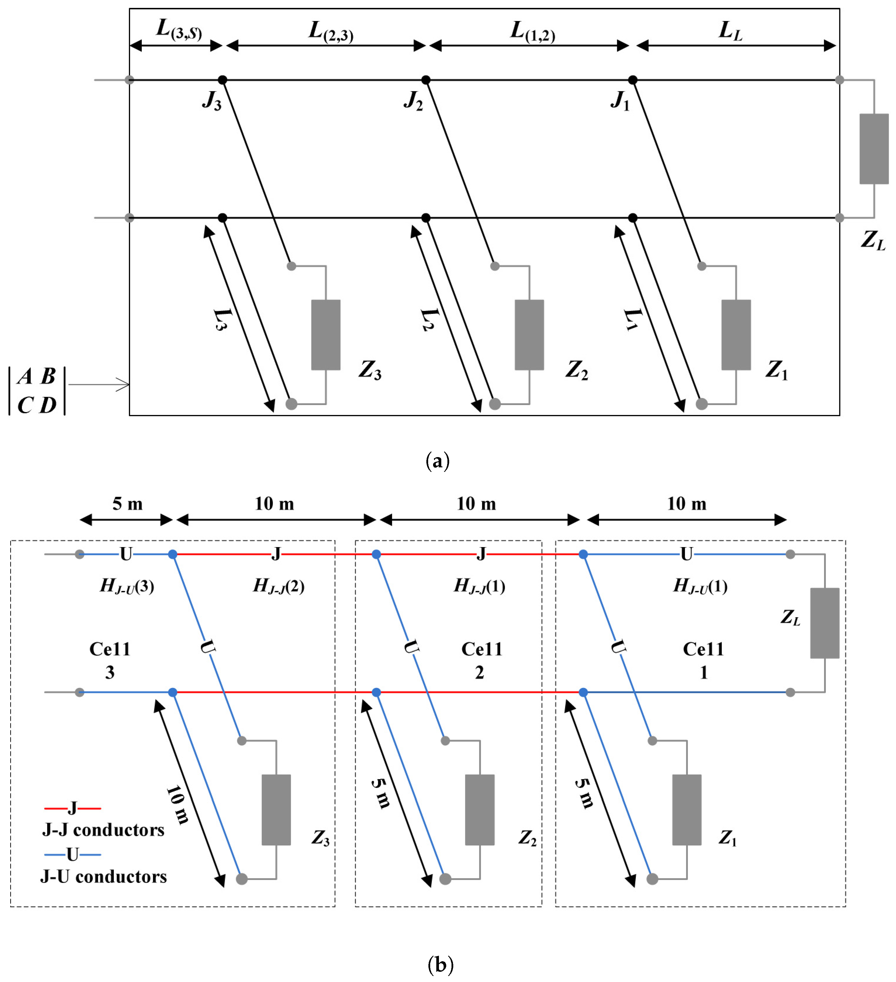
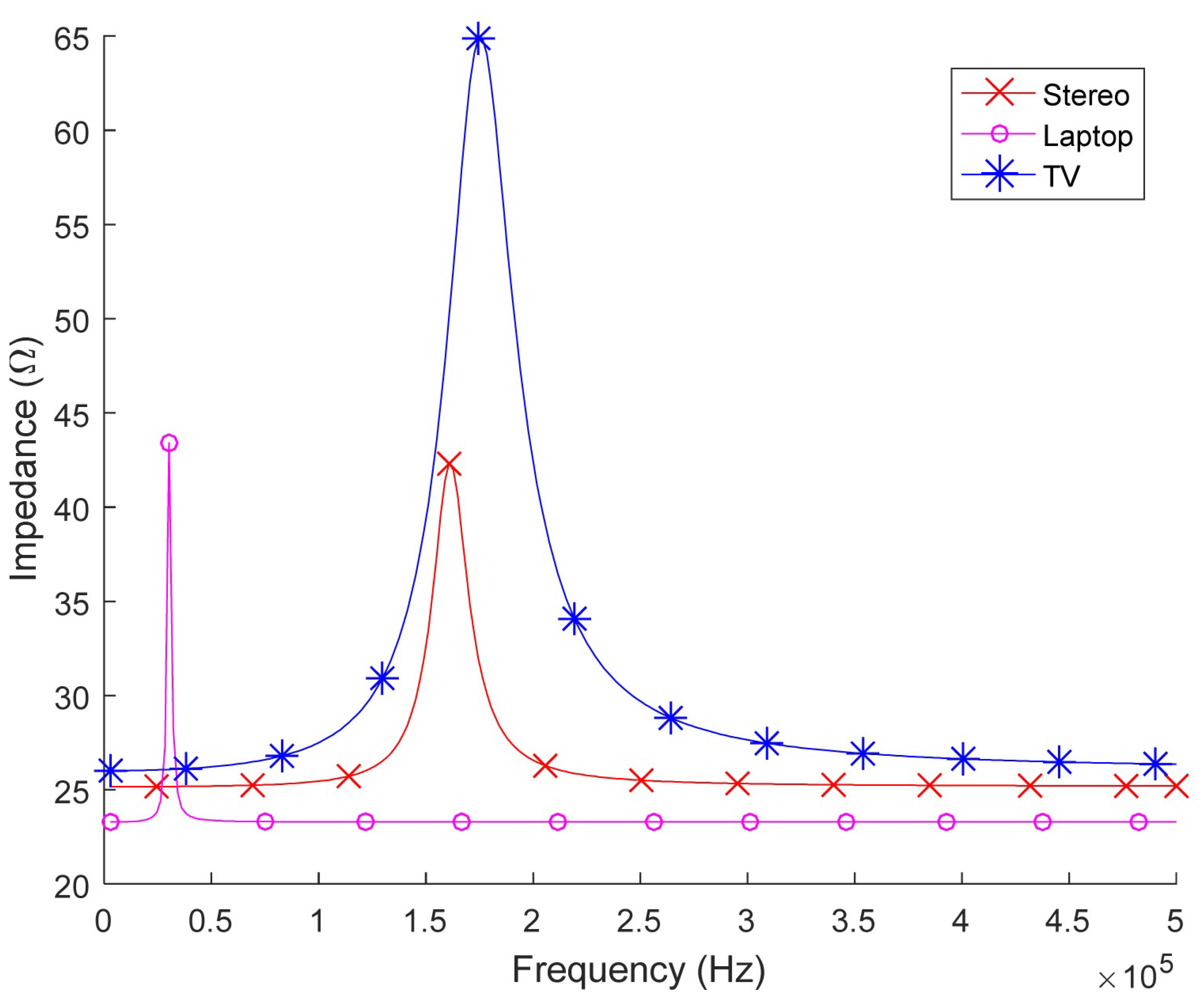
The Cañete wiring topology is a simple topology with 3 appliances as shown in Figure 12a [25]. This was modeled using the ABCD matrix method in [40]. The appliance parameters are given in

Table 6. Parameters for Three Appliances.

Appliance	Parameters
	${\mathit{P}}_{\mathit{r}}$ (VA)	${\mathit{f}}_0$ (kHz)	${\mathit{Q}}_{\mathit{f}}$
Stereo	243.0	161.3	9.0
Laptop	248.8	30.3	17.4
TV	261.1	175.4	5.6

and the corresponding impedances $\left|Z_i\right|$ are shown in Figure 13. At junction $J_i$, the input impedance of conductor $L_i$ is

$$Z_{ini}={\displaystyle \frac{A_i{Z}_i+B_i}{C_i{Z}_i+D_i}},$$

(22)

so the ABCD matrix of this topology is

$$\begin{array}{c}\left[\begin{array}{cc}A& B\\ C& D\end{array}\right]=\left[\begin{array}{cc}{A}_{(3,S)}& B_{(3,S)}\\ C_{(3,S)}& D_{(3,S)}\end{array}\right]\left[\begin{array}{cc}1& 0\\ 1/Z_{out3}& 1\end{array}\right]\left[\begin{array}{cc}{A}_{(2,3)}& B_{(2,3)}\\ C_{(2,3)}& D_{(2,3)}\end{array}\right]\left[\begin{array}{cc}1& 0\\ 1/Z_{out2}& 1\end{array}\right]\\ \times \left[\begin{array}{cc}{A}_{(1,2)}& B_{(1,2)}\\ C_{(1,2)}& D_{(1,2)}\end{array}\right]\left[\begin{array}{cc}1& 0\\ 1/Z_{out1}& 1\end{array}\right]\left[\begin{array}{cc}{A}_L& B_L\\ C_L& D_L\end{array}\right].\end{array}$$

(23)

The transfer function $H_T$ without considering $Z_S$ is [32]

$$H_T={\displaystyle \frac{Z_L}{A{Z}_L+B}}.$$

(24)

With the CD method, there are three cells in the topology as shown in Figure 12b. The impedance computation starts from cell 1 and proceeds to cell 3. The TFs of conductors $H_{J-U}\left(1\right)$, $H_{J-J}\left(1\right)$, $H_{J-J}\left(2\right)$, $H_{J-U}\left(3\right)$ were obtained and their product $H_b$ was computed using (18). Figure 14 shows that this provides the same IL as $H_T$ obtained from (24). However, the proposed method is flexible in modeling complex topologies, whereas the ABCD matrix method is not efficient as it uses a single matrix to represent the entire topology which is impractical.

6. Conclusions

In this paper, a power line communications (PLC) channel model was developed for a home area network (HAN) in the smart grid (SG). The use of PLC for smart meter (SM) communications and the associated standards were discussed. The wiring topology of a split-phase power system was modeled in detail and the parameters of the components within the topology were provided. Cell division (CD) was proposed as a bottom-up approach to obtain a channel model for a topology. This method uses the actual parameters of the topology components and thus provides an accurate model. Performance results were presented for three topology sizes, the three parts of the topology, normal breakers and advanced breakers, and individual and small appliance (SA) circuits. These show that the CD method is an efficient means of modeling HAN topologies. The CD method was also used to develop a model for the well known Cañete wiring topology, and this was compared with another method implemented on the same topology. The results indicate that the proposed method provides accurate channel models. This method can also be used to obtain channel models for other electrical systems such as electric vehicles or solar panels, and for any building topology.

As with other bottom-up approaches to developing channel models, the parameters of the components within the wiring topology must be obtained. However, these parameters can be estimated or randomly generated to obtain a more general model. Furthermore, the proposed model is efficient and flexible so that models with different components and parameters can easily be obtained. In the future, the models obtained can be used to evaluate HAN performance with PLC considering various modulation and medium access control techniques. The proposed technique can also be used to model the noise presents in a HAN. The influence of transient events (including plug in and removal events), can also be considered in the future.

References

- Fitzgerald, O.; Ugochukwu, B. Implementing the Paris Agreement: The Relevance of Human Rights to Climate Action; Centre for International Governance Innovation: Toronto, ON, Canada, 2016. [Google Scholar]
- Galli, S.; Scaglione, A.; Wang, Z. For the grid and through the grid: The role of power line communications in the smart grid. Proc. IEEE 2011, 99, 998–1027. [Google Scholar] [CrossRef]
- Adebisi, B.; Khalid, A.; Tsado, Y.; Honary, B. Narrowband PLC channel modelling for smart grid applications. In Proceedings of the 2014 9th International Symposium on Communication Systems, Networks & Digital Sign, Manchester, UK, 23–25 July 2014; pp. 67–72. [Google Scholar]
- Adebisi, B.; Treytl, A.; Haidine, A.; Portnoy, A.; Shan, R.; Lund, D.; Pille, H.; Honary, B. IP-centric high rate narrowband PLC for smart grid applications. IEEE Commun. Mag. 2011, 49, 46–54. [Google Scholar] [CrossRef]
- Haidine, A.; Adebisi, B.; Treytl, A.; Pille, H.; Honary, B.; Portnoy, A. High-speed narrowband PLC in smart grid landscape—State of the art. In Proceedings of the IEEE International Symposium on Power Line Communications and Its Applications, Udine, Italy, 3–6 April 2011; pp. 468–473. [Google Scholar]
- Yu, Q.; Johnson, R.J. Smart grid communications equipment: EMI, safety, and environmental compliance testing considerations. Bell Labs Tech. J. 2011, 16, 109–131. [Google Scholar] [CrossRef]
- Yussof, S.; Rusli, M.E.; Yusoff, Y.; Ismail, R.; Ghapar, A.A. Financial impacts of smart meter security and privacy breach. In Proceedings of the 6th International Conference on Information Technology and Multimedia, Putrajaya, Malaysia, 18–20 November 2014; pp. 11–14. [Google Scholar]
- Domínguez, J.; Chaves-Ávila, J.P.; Román, T.G.S.; Mateo, C. The economic impact of demand response on distribution network planning. In Proceedings of the Power Systems Computation Conference, Genoa, Italy, 20–24 June 2016; pp. 1–7. [Google Scholar]
- Pasdar, A.; Mirzakuchaki, S. A solution to remote detecting of illegal electricity usage based on smart metering. In Proceedings of the 2nd International Workshop on Soft Computing Applications, Oradea, Romania, 21–23 August 2007; pp. 163–167. [Google Scholar]
- Lin, Y.J.; Latchman, H.A.; Lee, M.; Katar, S. A power line communication network infrastructure for the smart home. IEEE Wirel. Commun. 2002, 9, 104–111. [Google Scholar] [Green Version]
- IEEE Standard for Broadband over Power Line Networks: Medium access Control and Physical Layer Specifications; IEEE Std 1901-2010; IEEE: Piscataway, NJ, USA, 2010; pp. 1–15.
- IEEE Standard for Low-Frequency Narrowband Power Line Communications for Smart Grid Applications; IEEE Std 1901.2-2013; IEEE: Piscataway, NJ, USA, 2013; pp. 1–35.
- Sharma, K.; Saini, L.M. Power line communications for smart grid: Progress, challenges, opportunities and status. Renew. Sustain. Energy Rev. 2017, 67, 704–751. [Google Scholar] [CrossRef]
- Panchadcharam, S.; Taylor, G.A.; Pisica, I.; Irving, M.R. Modeling and analysis of noise in power line communication for smart metering. In Proceedings of the IEEE Power and Energy Society General Meeting, San Diego, CA, USA, 22–26 July 2012; pp. 1–8. [Google Scholar]
- Sonmez, M.A.; Zehir, M.A.; Bagriyanik, M.; Nak, O. Impulsive noise survey on power line communication networks up to 125 kHz for smart metering infrastructure in systems with solar inverters in Turkey. In Proceedings of the International Conference on Renewable Energy Research and Applications, Madrid, Spain, 20–23 October 2013; pp. 705–710. [Google Scholar]
- Neagu, O.; Hamouda, W. Performance of smart grid communication in the presence of impulsive noise. In Proceedings of the International Conference on Selected Topics in Mobile Wireless Networking, Cairo, Egypt, 11–13 April 2016; pp. 1–5. [Google Scholar]
- Zhang, Z.; Qin, Z.; Zhu, L.; Weng, J.; Ren, K. Cost-friendly differential privacy for smart meters: Exploiting the dual roles of the noise. IEEE Trans. Smart Grid 2016, 8, 619–626. [Google Scholar] [CrossRef]
- Esmailian, T.; Kschischang, F.R.; Gulak, P.G. In-building power lines as high-speed communication channels: Channel characterization and a test channel ensemble. Int. J. Commun. Syst. 2003, 16, 381–400. [Google Scholar] [CrossRef]
- Galli, S.; Banwell, T. A deterministic frequency-domain model for the indoor power line transfer function. IEEE J. Sel. Areas Commun. 2006, 24, 1304–1316. [Google Scholar] [CrossRef] [Green Version]
- Banwell, T.; Galli, S. A novel approach to the modeling of the indoor power line channel Part I: Circuit analysis and companion model. IEEE Trans. Power Deliv. 2005, 20, 655–663. [Google Scholar] [CrossRef]
- Galli, S.; Banwell, T. A novel approach to the modeling of the indoor power line channel Part II: Transfer function and its properties. IEEE Trans. Power Deliv. 2005, 20, 1869–1878. [Google Scholar] [CrossRef]
- Marrocco, G.; Statovci, D.; Trautmann, S. A PLC broadband channel simulator for indoor communications. In Proceedings of the IEEE International Symposium on Power Line Communications and Its Applications, Johannesburg, South Africa, 24–27 March 2013; pp. 321–326. [Google Scholar]
- Nizigiyimana, R.; Lebunetel, J.; Raingeaud, Y.; Achouri, A.; Ravier, P.; Lamarque, G. Characterization and modeling breakers effect on power line communications. In Proceedings of the IEEE International Symposium on Power Line Communications and Its Applications, Glasgow, UK, 30 March–2 April 2014; pp. 36–41. [Google Scholar]
- Tonello, A.M.; Versolatto, F. Bottom-up statistical PLC channel modeling-Part I: Random topology model and efficient transfer function computation. IEEE Trans. Power Deliv. 2011, 26, 891–898. [Google Scholar] [CrossRef]
- Cañete, F.J.; Cortés, J.A.; Diez, L.; Entrambasaguas, J.T. A channel model proposal for indoor power line communications. IEEE Commun. Mag. 2011, 49, 166–174. [Google Scholar] [CrossRef]
- Earley, M.W.; Sargent, J.S.; Sheehan, J.V. National Electrical Code, 2014th ed.; National Fire Protection Association: Quincy, MA, USA, 2013; pp. 765–852. [Google Scholar]
- Versolatto, F.; Tonello, A.M. An MTL theory approach for the simulation of MIMO power-line communication channels. IEEE Trans. Power Deliv. 2011, 26, 1710–1717. [Google Scholar] [CrossRef]
- Rosa, E.B. The self and mutual inductances of linear conductors. Bull. Bur. Stand. 1907, 4, 301–344. [Google Scholar] [CrossRef]
- Dickinson, J.; Nicholson, P.J. Calculating the high frequency transmission line parameters of power cables. In Proceedings of the IEEE International Symposium on Power Line Communications and Its Applications, Essen, Germany, 2–4 April 1997; pp. 127–133. [Google Scholar]
- Miller, C.R. Illustrated Guide to the NEC, 6th ed.; Nelson Education: Toronto, ON, Canada, 2014; pp. 224–225. [Google Scholar]
- Hepler, D.J.; Wallach, P.R.; Hepler, D. Drafting and Design for Architecture and Construction, 9th ed.; Cengage Learning: Boston, MA, USA, 2012; pp. 675–683. [Google Scholar]
- Aalamifar, F.; Schlögl, A.; Harris, D.; Lampe, L. Modelling power line communication using network simulator-3. In Proceedings of the IEEE Global Communications Conference, Atlanta, GA, USA, 9–13 December 2013; pp. 2969–2974. [Google Scholar]
- Cavdar, I.H.; Engin, K. Measurements of impedance and attenuation at CENELEC bands for power line communications systems. Sensors 2008, 8, 8027–8036. [Google Scholar] [CrossRef] [PubMed]
- Sudiarto, B.; Widyanto, A.N.; Hirsch, H. Equivalent circuit identification of standby mode operation for some household appliances in frequency range 9–150 kHz for the investigation of conducted disturbance in low voltage installations. In Proceedings of the International Symposium on Electromagnetic Compatibility—EMC EUROPE, Wroclaw, Poland, 5–9 September 2016; pp. 835–838. [Google Scholar]
- Vines, R.M.; Trussell, H.J.; Shuey, K.C.; O’Neal, J.B., Jr. Impedance of the residential power-distribution circuit. IEEE Trans. Electromagn. Compat. 1985, 27, 6–12. [Google Scholar] [CrossRef]
- Ohm’s law and temperature resistance charts. Stud. Q. J. 1932, 3, 46–55. [CrossRef]
- Duffy, J.M.H.; Thomas, B. Frequency-Selective Circuit Protection Arrangements. U.S. Patent 6,437,955, 20 August 2002. [Google Scholar]
- Wilkinson, J.P. Nonlinear Resonant Circuit Devices. U.S. Patent 3,624,125, 16 July 1990. [Google Scholar]
- Neiger, B.B. Arc Fault Detector With Circuit Interrupter. U.S. Patent 6,088,205, 11 July 2000. [Google Scholar]
- Banwell, T.C.; Galli, S. On the symmetry of the power line channels. In Proceedings of the IEEE International Symposium on Power Line Communications and Its Applications, Malmö, Sweden, 4–6 April 2001; pp. 325–330. [Google Scholar]
Figure 1.
The average power consumption of residences.
Figure 2.
An example of the impedance carry back method using three steps in (a), (b) and (c), respectively [24].
Figure 3.
The topology above the panel.
Figure 4.
The topology of a 200 A panel.
Figure 5.
The circuit breaker model.
Figure 6.
A simple topology divided into cells.
Figure 7.
The average IL of the channels in the 1000 topologies for each house size.
Figure 8.
The IL of 8 random channels.
Figure 9.
The average IL of the three parts of the home topology.
Figure 10.
The average IL of the 9000 individual circuit channels and 8000 SA circuit channels in the 1000 topologies.
Figure 11.
The average IL with normal breakers and AFCI and GFCI breakers.
Figure 12.
The Cañete wiring topology modeled using (a) the ABCD matrix method, and (b) the cell division method.
Figure 13.
The impedances of the three appliances.
Figure 14.
The TFs of the Cañete wiring topology using two methods.